Projection of angular momentum via linear algebra

Abstract

Projection of many-body states with good angular momentum from an initial state is usually accomplished by a three-dimensional integral. We show how projection can instead be done by solving a straightforward system of linear equations. We demonstrate the method and give sample applications to ⁴⁸Cr and ⁶⁰Fe in the $pf$ shell. This new projection scheme, which is competitive against the standard numerical quadrature, should also be applicable to other quantum numbers such as isospin and particle number.

I Introduction

In the quantum theory of many-body systems we can have exact or nearly exact symmetries, sometimes referred to as ‘good’ symmetries, such as angular momentum, parity, isospin (for nuclear physics), and particle number. Breaking those good symmetries can paradoxically improve results and insights. In mean-field methods such as the Hartree-Fock (HF) approximation, deformed solutions often have lower energies than spherically symmetric solutions; number-mixing appproximations such as Hartree-Fock-Bogoliubov and Bardeen-Cooper-Schriefer also improve estimates of the ground state Ring and Schuck (2004).

To go even further, one wants to restore or project good quantum numbers, either before or after variation. (Henceforth we will restrict our discussion to angular momentum, though certainly our approach could be applied to other quantum numbers.) Angular momentum projection is typically accomplished by a three-dimension integral over the Euler angles Ring and Schuck (2004), using a complete, orthogonal set of angular functions.

We present an alternate approach which, instead of relying upon orthogonality, only needs two conditions: first, that the eigenfunctions of rotation are merely linearly independent, and second, that any initial state contains only a finite number of angular momenta. Under these two conditions projection of angular momentum in a finite space can be cast as solving a straightforward set of linear equations. The first condition is already trivially satisfied from orthogonality of the rotation matrices; and in a finite space not only can there be only a finite set of angular momentum eigenfunctions, in fact in most cases Slater determinants calculated from mean-field theory contain only a small fraction of the possible angular momentum states. Because of this small number we find linear algebra projection of angular momentum can be numerically competitive with the standard three-dimensional integral. Finally, we also discuss how the numerical efficiency can be improved by using the norm or overlap matrix elements to reduce the dimension of the linear algebra to be solved.

First we review the standard projection via quadrature over orthogonal functions. The most common projection operator uses the fact that rotation of a state of good total angular momentum $J$ and $z$-component $K$, (in nuclear physics, one often uses $K$ to denote the $z$-component of angular momentum in the so-called “intrinsic” frame Ring and Schuck (2004); here we use it to denote the $z$-component in the original frame, in order to better match common representations in the literature), does not mix total angular momentum $J$ but does mix the $z$ component Edmonds (1996):

$$\hat{R}(\alpha,\beta,\gamma)|J\,K\rangle=\sum_{M}{\cal D}^{(J)}_{M,K}(\alpha,\beta,\gamma)|J\,M\rangle,$$ (1)

where we have the the rotation operator over the Euler angles

$$\hat{R}(\alpha,\beta,\gamma)=\exp\left(i\gamma\hat{J}_{z}\right)\exp\left(i\beta\hat{J}_{y}\right)\exp\left(i\alpha\hat{J}_{z}\right),$$ (2)

with $\hat{J}_{z}$ and $\hat{J}_{y}$ the generators of rotations about the $z$ and $y$-axes, respectively, and where ${\cal D}^{(J)}_{M,K}$ is a Wigner D-matrix. The Wigner $D$-matrices are the matrix elements of the the rotation operator in a basis of good angular momentum, and can be shown to be eigenfunctions of the quantized symmetric top Edmonds (1996) and form a complete orthogonal set,

$$\int_{0}^{2\pi}d\alpha\int_{0}^{\pi}\sin\beta d\beta\int_{0}^{2\pi}d\gamma\,{\cal D}^{(J^{\prime})*}_{M^{\prime},K^{\prime}}(\alpha,\beta,\gamma){\cal D}^{(J)}_{M,K}(\alpha,\beta,\gamma)=\frac{8\pi^{2}}{2J+1}\delta_{J,J^{\prime}}\delta_{M,M^{\prime}}\delta_{K,K^{\prime}},$$ (3)

a property which can be exploited for angular momentum projection. Consider some initial state which is a mixture of states of good angular momenta:

$$|\Psi\rangle=\sum_{J,\lambda}c_{J,\lambda}|\psi:J\lambda,K_{\lambda}\rangle.$$ (4)

We use $\lambda$ to distinguish components with the same $J$ but different initial $K_{\lambda}$; in general these will not be eigenstates of the Hamiltonian. Then applying the rotation operator,

$$\hat{R}(\alpha,\beta,\gamma)|\Psi\rangle=\sum_{J,\lambda}c_{J,\lambda}\sum_{M}{\cal D}^{(J)}_{M,K_{\lambda}}(\alpha,\beta,\gamma)|\psi:J\lambda,M\rangle,$$ (5)

where we use $K_{\lambda}$ to denote the value of $J_{z}$ in the original state, and $M$ in rotated states. The reason we do this is in the expansion (4), if we rotate states with the same $J$ and different $\lambda$ to have the same orientation, they need not be orthogonal to each other, that is, $\langle\psi:J\lambda,M|\psi:J\mu,M\rangle$ does not need to vanish when $\lambda\neq\mu$. To project angular momentum, we rotate all components of (4) to have the same orientation $M$. This leads to the standard angular momentum projection equations Ring and Schuck (2004): one constructs the norm matrix

$$N^{J}_{MK}=\frac{8\pi^{2}}{2J+1}\int d\Omega\,{\cal D}^{(J)*}_{M,K}(\Omega)\left\langle\Psi\left|\hat{R}(\Omega)\right|\Psi\right\rangle$$ (6)

where $\Omega$ stands in for the Euler angles $\alpha,\beta,\gamma$. The norm matrix can be can be written in terms of the expansion (4):

$$N^{J}_{MK}=\sum_{\lambda\mu}\delta_{M,K_{\lambda}}c^{*}_{J,\lambda}c_{J,\mu}\langle\psi:J\lambda,M|\psi:J\mu,M\rangle.$$ (7)

We can do the same for the Hamiltonian matrix

$$H^{J}_{MK}=\frac{8\pi^{2}}{2J+1}\int d\Omega\,{\cal D}^{(J)*}_{M,K}(\Omega)\left\langle\Psi\left|\hat{H}\hat{R}(\Omega)\right|\Psi\right\rangle$$ (8)

$$=\sum_{\lambda\mu}\delta_{M,K_{\lambda}}c^{*}_{J,\lambda}c_{J,\mu}\langle\psi:J\lambda,M|\hat{H}|\psi:J\mu,M\rangle,$$

where $\hat{H}$ is the many-body Hamiltonian. One then solves for each $J$ the generalized eigenvalue problem, with solutions labeled by $r$

$$\sum_{K}H^{J}_{MK}g^{(J)}_{K,r}=E_{r}\sum_{K}N^{J}_{M,K}g^{(J)}_{K,r},$$ (9)

with the reconstructed eigenfunction

$$|\Psi JM,r\rangle=\sum_{K}g^{(J)}_{K,r}\int d\Omega\,{\cal D}^{(J)*}_{M,K}(\Omega)|\Psi\rangle$$ (10)

$$=\sum_{K}g^{(J)}_{K,r}\sum_{\lambda}\delta_{K,K_{\lambda}}c_{J,\lambda}|\psi:J\lambda,M\rangle.$$

If one projects from a single initial state, for each $J$ there are at most $2J+1$ unique solutions; the number of actual unique solutions corresponds to the number of nonzero eigenvalues of the matrix $\mathbf{N}^{J}$, although in many applications one projects on multiple initial states.

Some of the many applications are projected Hartree-Fock Ring and Schuck (2004); Gunye and Warke (1967) including variation after projection Ring and Schuck (2004); Rodríguez et al. (2005), and Hartree-Fock-Bogoliubov Ring and Schuck (2004); Sheikh and Ring (2000); Borrajo and Egido (2016); the Monte Carlo Shell Model Honma et al. (1996); Abe et al. (2013); the projected shell model Hara and Sun (1995); Sun and Hara (1997); Sheikh and Hara (1999); the projected configuration-interaction Gao and Horoi (2009) and related methods Schmid (2004); and projected generator coordinate Rodríguez-Guzmán et al. (2002); Yao et al. (2010). This list is far from exhaustive.

The matrices $N^{J}_{MK}$ and $H^{J}_{MK}$ are generally small in dimension, but to arrive at them one needs to evaluate the integrand matrix elements $\left\langle\Psi\left|\hat{R}(\Omega)\right|\Psi\right\rangle$ and $\left\langle\Psi\left|\hat{H}\hat{R}(\Omega)\right|\Psi\right\rangle$ for a large number of angles $\Omega$. As an example, a recent paper Borrajo and Egido (2016) used 32 points per Euler angle, or a total of $32^{3}=32,768$ angles. If one imposes symmetries, i.e. axial symmetry, upon the mean-field state one can reduce the number of evaluations Hara and Sun (1995), but even so each evaluation is computationally intensive, especially of the Hamiltonian; see section V.

Projecting out from fully triaxial states, or projecting additional quantum numbers such as isospin or particle number, is so computationally intensive one often has to severely restrict the model space Gao et al. (2015). Given the applications of angular momentum projection and the computational burden, we were motivated to find an alternate approach, not by speeding up the evaluation of the integrands for any set of Euler angles, but rather to reduce the number of mesh points needed.

II Linear algebra solution for angular momentum projection

Equations (6) and (8) are usually taken as recipes for computing the norm and Hamiltonian matrices, respectively. We ignore the integrals, instead taking (7) and (8) them as definitions of those matrices in terms of the expansion (4). Starting from Eqn. (5) and using those definitions, one finds for any given value of the Euler angles $\Omega=(\alpha,\beta,\gamma)$,

$$\langle\Psi|\hat{R}(\Omega)|\Psi\rangle=\sum_{J,K,M}{\cal D}^{(J)}_{M,K}(\Omega)N^{J}_{MK},$$ (11)

$$\langle\Psi|\hat{H}\hat{R}(\Omega)|\Psi\rangle=\sum_{J,K,M}{\cal D}^{(J)}_{M,K}(\Omega)H^{J}_{MK}.$$ (12)

These key equations say $\langle\Psi|\hat{R}(\Omega)|\Psi\rangle$ is a linear combination of the the norm matrix elements $N^{J}_{MK}$, and the same for $\Psi|\hat{H}\hat{R}(\Omega)|\Psi\rangle$ and the Hamiltonian matrix elements $H^{J}_{MK}$. While in usual practice one uses the orthogonality of the ${\cal D}$-matrices, Eq.  (3), to find $N^{J}_{MK}$, $H^{J}_{MK}$, we instead rely only upon their linear independence and solve solve Eqn. (11) and (12) as a linear algebra problem. That is, if we label a particular choice of Euler angles $\Omega$ by $i$ and the angular momentum quantum numbers $J,M,K$ by $a$, and define

$$n_{i}\equiv\langle\Psi|\hat{R}(\Omega_{i})|\Psi\rangle,$$

$$D_{ia}\equiv{\cal D}^{(J_{a})}_{M_{a},K_{a}}(\Omega_{i}),$$ (13)

$$N_{a}\equiv N^{J_{a}}_{M_{a}K_{a}},$$

we can rewrite Eq. (11) simply as

$$n_{i}=\sum_{a}D_{ia}N_{a}$$ (14)

which can be easily solved for $N_{a}=N^{J}_{M,K}$, as long as $D_{ia}$ is invertible, with a similar rewriting of Eq. (12) and solution for $H^{J}_{M,K}$.

A key idea is that the sums (11), (12) are finite. To justify this, we introduce the fractional ‘occupation’ of the wave function with angular momentum $J$, which is the trace of the fixed-$J$ norm matrix:

$$f_{J}=\sum_{M}N^{J}_{M,M}.$$ (15)

Assuming the original state is normalized, one trivially has

$$\sum_{J}f_{J}=1.$$ (16)

The fractional occupation $f_{J}$ and its sum rule (16) have multiple uses. First, the sum rule is an important check on any calculation. Second and more important, one can use the exhaustion of the sum rule to determine a maximum angular momentum, $J_{\mathrm{max}}$, in our expansions; in our trials we found both (4) and (16) dominated by a finite and relatively small number of terms, far fewer terms than are allowed even in finite model spaces. As discussed in the next section, we found that fractional occupations below $0.001$ could be safely ignored.

In general, for a Hartree-Fock state the distribution of $f_{J}$ is weighted towards low $J$ and does not reach the maximum $J$ in the many-body space. In Fig. 1 we show this for ⁶⁰Fe in the $pf$ shell where the maximum $J$ in the space is $26$, using the $pf$-shell interaction derived from a $G$-matrix, version A, or GXPF1A Honma et al. (2002, 2005). We also show the distribution of $f_{J}$ for a strongly cranked Slater determinant, where we added $\hbar\omega J_{z}$ (or, alternately, $J_{x}$) with $\hbar\omega=1.0$ MeV. For uncranked Hartree-Fock the maximum $J$ is 12 with an $f_{J}\sim 0.001$; because the Hartree-Fock state is axially symmetric, only even $J$ were populated. For the strongly cranked Hartree-Fock state, most of the state had $J=12$, but the range was between 6 and 16. Because the cranked HF state was triaxial we also got odd $J$.

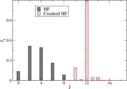
Figure 1: (Color online) Fraction of given angular momentum $J$ ($f_{J}$) in a Slater determinant, calculated both for ordinary Hartree-Fock (HF) and cranked HF with cranking frequency $\hbar\omega=1.0$ MeV, for ⁶⁰Fe in the $pf$ shell. The maximum angular momentum for this nuclide in this model space is 26 $\hbar$.

Our method is not completely unprecedented. For example, previous applications in the so-called shell-model Monte Carlo extracted traces over states with good particle number Ormand et al. (1994) and good $M$ ($z$-component of angular momentum) Alhassid et al. (2007) via Fourier methods which can be thought of as inverting the linear relation analytically. To the best of our knowledge, however, this is the first time one has fully projected out angular momentum using inversion of linear equations.

III Implementation

To implement projection by linear algebra, we worked in finite single-particle shell-model spaces, such as the $pf$ shell. We used the code SHERPA Stetcu and Johnson (2002); Stetcu (2003) to generate unrestricted Hartree-Fock states $|\Psi_{HF}\rangle$; SHERPA reads in shell-model configuration-interaction compatible files, and can handle even and odd number of protons and neutrons, and allows for arbitrary triaxility. We then projected out the norm and Hamiltonian matrices using both quadrature and linear inversion.

There are two practical choices which must be made. The first is one of tolerance of small values; the second is the choice of mesh of Euler angles for evaluating matrix elements.

When solving the generalized eigenvalue equation (9), the norm matrix often is not formally invertible, because it has eigenvalues which either are zero or are very small. Such tiny eigenvalues generally have numerical noise and including them leads to unphysical solutions. Hence one needs to choose a tolerance $\epsilon$; for any eigenvalues less than $\epsilon$ we exclude the associated subspace. We found a tolerance of $\epsilon\sim 0.001$ worked satisfactorily. One also has to choose a tolerance for satisfying the sum rule (16). This essentially dictates the maximal $J$ used in inversions. Again, we found that a tolerance of $\sim 0.001$ worked satisfactorily, that is, $\sum_{J}^{J_{\mathrm{max}}}f_{J}\geq 0.999$ determined $J_{\mathrm{max}}$.

In order to solve for the projected Hamiltonian and norm matrices, one must first choose a mesh of Euler angles such that the linear equations are solvable. For our initial inversions, we found a simple mesh, which allowed us to invert each Euler angle separably, worked well. To simplify our solution, we solved for each each quantum number $J,K,M$ separately. To make clear this approach, we we expand (14) to read

$$n_{ijk}=\sum_{JKM}D_{ijk,JKM}N^{J}_{KM}$$ (17)

where

$$n_{ijk}\equiv\langle\Psi|\exp(i\alpha_{i}\hat{J}_{z})\exp(i\beta_{j}\hat{J}_{y})\exp(i\gamma_{k}\hat{J}_{z})|\Psi\rangle$$

$$=\sum_{JKM}D^{J}_{K,M}(\alpha_{i},\beta_{j},\gamma_{k})\,N^{J}_{K,M}$$

$$=\sum_{JKM}e^{i\alpha_{i}M}d^{J}_{MK}(\beta)e^{i\gamma_{k}K}\,N^{J}_{K,M}$$ (18)

where $d^{J}_{MK}(\beta)$ is of course the Wigner little-$d$ function. By separable we mean the Euler angles $\alpha_{,}\beta_{j},\gamma_{k}$ run independent of each other and we solve (17) one index at a time. To begin with, we use on the angles $\alpha,\gamma$ an equally spaced mesh $\gamma_{k}=(k-1)\frac{2\pi}{2J_{\mathrm{max}}+1},k=1,2J_{\mathrm{max}}+1$, (and similarly for $\alpha_{i}$). We analytically invert the finite Fourier sums using Alhassid et al. (2007)

$$\frac{1}{N}\sum_{k=1}^{N}\exp\left(i\frac{2\pi Mk}{N}\right)=\delta_{M,0}.$$ (19)

and introduce the matrix

$$Z_{Kk}=\frac{1}{2J_{\mathrm{max}}+1}\exp(-iK\gamma_{k}).$$ (20)

to arrive at the intermediate quantity

$$n_{j,MK}=\sum_{ik}Z_{Mi}Z_{Kk}N_{ijk}=\sum_{J}d^{J}_{MK}(\beta_{j})N^{J}_{MK}.$$ (21)

At this point we have done two-thirds of the work. We have ‘projected’ the magnetic quantum numbers $K$ and $M$; all that remains is to project out total $J$.

To obtain projection on total $J$, we also need a mesh on $\beta$. We chose an equally spaced mesh on $\beta_{j}$:

$$\beta_{j}=(j-1)\frac{\pi}{N},$$ (22)

where $N=J_{\mathrm{max}}+1$ if an even system and $=J_{\mathrm{max}}+1/2$ if an odd number of nucleons. To invert, construct

$$\Delta^{J^{\prime}J}_{MK}=\sum_{j}d^{J^{\prime}}_{MK}(\beta_{j})d^{J}_{MK}(\beta_{j}),$$ (23)

with $J,J^{\prime}\geq|M|,|K|$. (This step is inspired by singular value decomposition treatment of nonsquare matrices, although we are not formally carrying out singular value decomposition.) The matrix $\Delta^{J^{\prime}J}$ is real and symmetric with fixed $M,K$. We numerically confirmed, for $J\geq\max(|K|,|M|)$, it is invertible and has nonzero (and nonnegative) eigenvalues. We construct another intermediate matrix,

$$\tilde{N}_{J^{\prime},MK}=\sum_{j}d^{J^{\prime}}_{MK}(\beta_{j})N_{j,MK}.$$ (24)

Then we simply solve

$$\sum_{J}\Delta^{J^{\prime}J}_{MK}N^{J}_{MK}=\tilde{N}_{J^{\prime},MK}.$$ (25)

In a similar fashion we solved for $H^{J}_{KM}$ and then could solve Eq. (9). We confirmed our matrices were the same using either quadrature of linear algebra to project.

IV Example applications

Table 1: Low-lying energies, in MeV, of ⁴⁸Cr from projected Hartree-Fock in the $pf$ shell with the interaction GX1A. $f_{J}$ is the fraction of the Hartree-Fock state with angular momentum $J$, eqn. (15). ‘quad’ refers to projection by quadrature, eqn. (6) and (8) and the number of points, while ‘LAP’ refers to linear algebra projection.

$\,\,J\,\,$	$f_{J}$	quad.	quad.	LAP	LAP
		20 pts	40 pts	(full)	(‘need-to-know’ )
0	0.0695	-97.9760	-97.9778	-97.9778	-97.9775
2	0.2817	-97.5024	-97.5044	-97.5044	-97.5037
4	0.3115	-96.5570	-96.5522	-96.5522	-96.5520
6	0.2077	-95.2162	-95.1115	-95.1115	-95.1114
8	0.0935	-104.2016	-93.3330	-93.3330	-93.3325
10	0.0292	-133.9126	-91.1718	-91.1719	-91.1717
12	0.0069	-141.5208	-88.8433	-88.8499	-88.8558

We give two brief example applications of the method, both in the $pf$ shell. The first, ⁴⁸Cr, shows the level of agreement between projection by quadrature and linear algebra projection. We have done numerous other tests in other nuclei and other model spaces, including multi-shell spaces, and find similar agreement. The second exhibits good agreement of yrast excitation energies in ⁶⁰Fe between full shell-model diagonalization and linear algebra projected Hartree-Fock.

Table 1 shows the low-lying projected Hartree-Fock spectra of ⁴⁸Cr computed in the $pf$ shell with GXPF1A Honma et al. (2002, 2005). We show four calculations, two quadrature calculations with 20 and 40 points, and two linear algebra projection (LAP) calculations, one with a full inversion and one with the ‘need-to-know’ modification described in section V. The quadrature calculation with 40 points on each angle, or $40^{3}=64,000$ evaluations agrees with both the full LAP (12,615 evaluations) and the need-to-know (4,375 evaluations) to within 2 keV, except for the $J=12$ state, which agreed within $\sim 10$ keV. (This latter had a fractional occupation $f_{J}=0.007$, close to our tolerance, and in general we found less reliable results in both quadrature and LAP for states with tiny fractional occupations.) The quadrature calculation with 20 points on each angle, or 8000 evaluations, agrees for small $J$ but breaks down for larger angular momentum; although we don’t show it, this breakdown is also signaled by a failure in the sum rule (16).

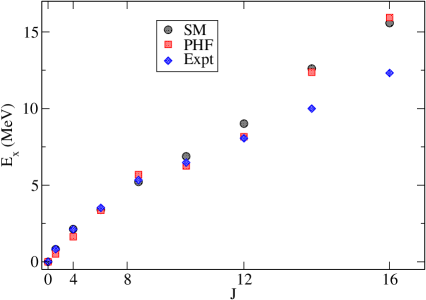
Figure 2: (Color online) Yrast excitation energies for ⁶⁰Fe computed in the $pf$ shell with the semi-phenomenological interaction GXPF1A. Results are from full shell-model diagonalization (SM, black circles) and linear algebra projected Hartree-Fock (PHF, red squares). For comparison we also show the experimental values (blue diamonds). .

The other demonstration is of the yrast excitation energies of ⁶⁰Fe, shown in Fig. 2, also computed in the $pf$ shell with the GXPF1A interaction. We compare results from full shell-model diagonalization (black circles), also known as configuration-interaction method, against our LAP projected Hartree-Fock results (red squares). For such a simple calculation we get good agreement between the two calculations, although both diverge at high $J$ from experiment (blue diamonds).

Although we have shown only even-even cases, LAP works just fine for odd-$A$ and odd-odd cases. Of course, projected Hartree-Fock spectra do not always provide a good approximation to equivalent full shell-model diagonalization. Unsurprisingly the best agreement was for rotational spectra of even-even nuclei. We plan to study this more systematically in the future. In general the PHF spectra for even-even nuclei better approximate the numerically exact results; in addition, systems with an odd number of particles generally mix in all values of $J$ and $M$, thus making the need-to-know algorithm less applicable. Nonetheless, we have found excellent agreement between quadrature projection and LAP for odd-$A$ and odd-odd nuclei.

We carried out similar explorations for many nuclides in the $sd$- and $pf$ shells, in the $sd$-$pf$ space, in the $0g_{7/2}$-$1d$-$2s$-$0g_{11/2}$ space, and in a no-core shell model space including all orbits up to principal quantum number $N=5$. This included odd-$A$ and odd-odd nuclides. Qualitatively all results were similar to Fig. 1, and without cranking we seldom found $f_{J}>0.001$ for $J>16$. (In spaces including opposite parity orbits we also projected on parity, by taking $|\Psi\rangle\pm P|\Psi\rangle$ where $P$ is the parity inversion operator.) Only when we cranked did we get large $J$, but in those cases the distribution was again clustered on a relatively small number of $J$ values.

V Computational burden and improved efficiency through ‘need to know’

The motivation for introducing this new algorithm is to reduce the computational burder of projecting good quantum numbers. In this section we discuss the origin and scaling of the computational burden and outline an advanced algorithm with even greater efficiency.

Let’s briefly overview some details on computing matrix elements in this particular framework Lang et al. (1993). Suppose, starting from $N_{s}$ orthonormal single-particle basis states $\phi_{a}$, $a=1,N_{s}$, represented by creation and destruction operators $\hat{c}^{\dagger}_{a},\hat{c}_{a}$, we construct general single-particle states $\sum_{a}\Psi_{ai}\phi_{a}$, $i=1,N_{p}$. Then we can represent the Slater determinant which is the antisymmetrized product of these $N_{p}$ states by the $N_{s}\times N_{p}$ matrix $\mathbf{\Psi}$, even if the column vectors are not orthonormal. The overlap between two such general Slater determinants is $\langle\Psi|\Psi^{\prime}\rangle=\det\mathbf{\Psi}^{\dagger}\mathbf{\Psi}^{\prime}$; computing the matrix $\mathbf{\Psi}^{\dagger}\mathbf{\Psi}^{\prime}$ is of the order of $N_{p}^{2}N_{s}$ operations, while the determinant can be computed using LU decomposition and takes on the order of $N_{p}^{3}$ operations. As long as the two Slater determinants are not orthogonal to each other, the one-body density matrix is $\rho_{ab}=\langle\Psi|\hat{c}^{\dagger}_{a}\hat{c}_{b}|\Psi\rangle=(\mathbf{\Psi^{\prime}}(\mathbf{\Psi}^{\dagger}\mathbf{\Psi}^{\prime})^{-1}\Psi^{\prime})_{ba}$, and the (normalized) matrix element of a two-body operator $\hat{V}=\sum_{abcd}V_{abcd}\hat{c}^{\dagger}_{a}\hat{c}^{\dagger}_{b}\hat{c}_{d}\hat{c}_{c}$ is $\langle\Psi|\hat{V}|\Psi\rangle/\langle\Psi|\Psi^{\prime}\rangle=\sum_{abcd}V_{abcd}(\rho_{ac}\rho_{bd}-\rho_{ad}\rho_{bc})$. This last sum, which goes roughly like $N_{s}^{4}$ (though some matrix elements are zero by selection rules), and because $N_{s}>N_{p}$ it is evalution of the Hamiltonian that is computationally burdensome. For more detailed exposition on this, see Stetcu and Johnson (2002); Lang et al. (1993) and references therein. In other frameworks, i.e., coordinate space mean-field calculations, the analysis may be different.

As in our implementation, the norm matrix elements are far cheaper than the Hamiltonian, we devised a ‘need to know’ methodology: (1) using a large $J_{\mathrm{max}}$, compute the norm matrix elements and the $f_{J}$, confirming that the sum rule (16) is satisfied; (2) using some cutoff $f_{\mathrm{min}}$, selected the occupied values of $J$ such that $f_{J}>f_{\mathrm{min}}$, typically around $10^{-3}$; (3) solve (11) and (12) but using only the occupied values of $J$ in the sum. This means fewer terms in the expansion and thus a corresponding smaller number of Euler angles $\Omega_{i}$ at which to evaluate the computationally expensive left-hand side of (12) in particular.

We can sketch out the comparative computational burden. For most of our cases, we found quadrature meshes between $25^{3}=15,625$ Euler angles and $32^{3}=32,768$ angles were sufficient. Suppose we have a $J_{\mathrm{max}}=12$. In the simplest possible mesh for linear algebra projection (LAP), $J$ runs from 0 to 12, and f $M,K$ run between -12 and 12; thus the number of evaluations are $13\times 25\times 25=8125$ Euler angles, or lbetween half and a quarter as many evaluations required as for quadrature. In fact, this is overcounting: the minimal number of evaluations should be, for each occupied value of $J$, a sum over all combinations of allowed $M$ and $K$ or $2J+1$ for each, that is, $\sum_{J=0}^{J_{\mathrm{max}}}(2J+1)^{2}\approx(4/3)J_{\mathrm{max}}^{3}$ which is a factor of 3 smaller still. While we have not yet implemented such a minimal mesh for LAP, we did implement a ‘need to know’ mesh. For example, if one has only even $J$ values, then the number of evaluations is half as much. This involves inverting $\Delta_{KM}^{J^{\prime}J}$ only for select values of $J^{\prime},J$. We gave such an example for ⁴⁸Cr in section IV.

We found, however, the invertibility of the matrix $\Delta_{KM}^{J^{\prime}J}$ as defined in Eq. (23) is surprisingly sensitive to both the choice of $J$s and to the angles $\beta_{i}$. We succeeded in the case of ⁴⁸Cr, by taking only the even values of $J,J^{\prime}$ and skipping every other value of $\beta_{i}$ in the mesh (22), but in other cases we were not successful. Fortunately the invertibility is easy to know, as it depends upon the eigenvalues of the symmetric matrix $\Delta_{KM}^{J^{\prime}J}$. We found as long as the eigenvalues were $>10^{-4}$ we got good results. While further investigation is needed, this approach looks promising.

VI Conclusions and future work

We have proposed and demonstrated a new method of projecting angular momentum using linear algebra. Our initial implementation demonstrates the method works and, for moderately high angular momentum $J$, is computationally competitive, in many cases requiring significantly fewer evaluations than standard quadrature methods. While for our demonstrations we mostly used the most straightforward separable inversion, we demonstrated a ‘need-to-know’ inversion, where one computed the fractional occupations $f_{J}$ via the norm matrix and then used a reduced sampling for extracting the computationally expensive Hamiltonian matrix. Because the inversion becomes sensitive to the choice of angles, further investigation into these improved inversions is suggested. We also leave to future work application to systems beyond shell-model spaces (i.e., coordinate-space mean-field wave functions), to cases with multiple initial states, e.g., generator-coordinator and relative methods, to transitions, and other finite quantum numbers such as isospin and particles number Gao et al. (2015).

This material is based upon work supported by the U.S. Department of Energy, Office of Science, Office of Nuclear Physics, under Award Number DE-FG02-96ER40985, as well as internal funding from San Diego State University to support one of us (O’Mara) for summer research. The implementation of angular momentum projection via quadrature was modified from a prior, unpublished version by J. T. Staker. CWJ would also like to thank Changfeng Jiao for inspiring discussions.

References

- Ring and Schuck (2004) P. Ring and P. Schuck, The nuclear many-body problem (Springer Science & Business Media, 2004).
- Edmonds (1996) A. R. Edmonds, Angular momentum in quantum mechanics (Princeton University Press, 1996).
- Gunye and Warke (1967) M. R. Gunye and C. S. Warke, Phys. Rev. 156, 1087 (1967).
- Rodríguez et al. (2005) T. R. Rodríguez, J. L. Egido, L. M. Robledo, and R. Rodríguez-Guzmán, Phys. Rev. C 71, 044313 (2005).
- Sheikh and Ring (2000) J. A. Sheikh and P. Ring, Nuclear Physics A 665, 71 (2000).
- Borrajo and Egido (2016) M. Borrajo and J. L. Egido, The European Physical Journal A 52, 277 (2016).
- Honma et al. (1996) M. Honma, T. Mizusaki, and T. Otsuka, Phys. Rev. Lett. 77, 3315 (1996).
- Abe et al. (2013) T. Abe, P. Maris, T. Otsuka, N. Shimizu, Y. Tsunoda, Y. Utsuno, J. Vary, and T. Yoshida, in Journal of Physics: Conference Series, Vol. 454 (IOP Publishing, 2013) p. 012066.
- Hara and Sun (1995) K. Hara and Y. Sun, International Journal of Modern Physics E 4, 637 (1995).
- Sun and Hara (1997) Y. Sun and K. Hara, Computer physics communications 104, 245 (1997).
- Sheikh and Hara (1999) J. A. Sheikh and K. Hara, Phys. Rev. Lett. 82, 3968 (1999).
- Gao and Horoi (2009) Z.-C. Gao and M. Horoi, Phys. Rev. C 79, 014311 (2009).
- Schmid (2004) K. Schmid, Progress in Particle and Nuclear Physics 52, 565 (2004).
- Rodríguez-Guzmán et al. (2002) R. Rodríguez-Guzmán, J. L. Egido, and L. M. Robledo, Phys. Rev. C 65, 024304 (2002).
- Yao et al. (2010) J. M. Yao, J. Meng, P. Ring, and D. Vretenar, Phys. Rev. C 81, 044311 (2010).
- Gao et al. (2015) Z.-C. Gao, M. Horoi, and Y. S. Chen, Phys. Rev. C 92, 064310 (2015).
- Honma et al. (2002) M. Honma, T. Otsuka, B. A. Brown, and T. Mizusaki, Phys. Rev. C 65, 061301 (2002).
- Honma et al. (2005) M. Honma, T. Otsuka, B. Brown, and T. Mizusaki, Eur. Phys. J. A 25, 499 (2005).
- Ormand et al. (1994) W. E. Ormand, D. J. Dean, C. W. Johnson, G. H. Lang, and S. E. Koonin, Phys. Rev. C 49, 1422 (1994).
- Alhassid et al. (2007) Y. Alhassid, S. Liu, and H. Nakada, Phys. Rev. Lett. 99, 162504 (2007).
- Stetcu and Johnson (2002) I. Stetcu and C. W. Johnson, Phys. Rev. C 66, 034301 (2002).
- Stetcu (2003) I. Stetcu, TOWARD A GLOBAL MICROSCOPIC THEORY FOR NUCLEAR STRUCTURE: MEAN FIELD PLUS RANDOM PHASE APPROXIMATION VS. SHELL MODEL, Ph.D. thesis, Louisiana State University (2003).
- Lang et al. (1993) G. H. Lang, C. W. Johnson, S. E. Koonin, and W. E. Ormand, Phys. Rev. C 48, 1518 (1993).