Higher order string effects and the properties of the Pomeron

Abstract

We revisit the description of the Pomeron within the effective string theory of QCD. Using a string duality relation, we show how the static potential maps onto the high-energy scattering amplitude that exhibits the Pomeron behavior. Besides the Pomeron intercept and slope, new additional terms stemming from the higher order string corrections are shown to affect both the growth of the nucleon’s size at high energies and its profile in impact parameter space. The stringy description also allows for an odderon that only disappears in critical dimension. Some of the Pomeron’s features that emerge within the effective string description can be studied at the future EIC collider.

I Introduction

Hadron-hadron scattering at high energy is dominated by the exchange of weakly interacting Pomerons and Reggeons with vacuum and meson quantum numbers respectively. Many decades ago, a description of this process within the effective Reggeon field theory was pioneered by Gribov and collaborators Gribov:1973jg .

A first principle approach to Reggeon physics in the context of weakly coupled QCD was succesfully obtained by re-summing rapidity ordered Feynman graphs Kuraev:1977fs . The BFKL Pomeron Kuraev:1977fs emerges in leading order through the re-summed two-gluon ring diagrams with vacuum quantum numbers. Few non-perturbative approaches to Reggeon physics in the context of QCD have also been attempted, ranging from the stochastic vacuum PIRNER to a Reggeized graviton in holography Brower:2006ea . Here, we will be interested in the Pomeron as a semi-classical stringy instanton or in short the BKYZ Pomeron Basar:2012jb .

The BKYZ Pomeron carries intrinsic temperature and entropy Shuryak:2013sra , i.e. $T=\chi/(2\pi b)$ with $\chi={\rm ln}(s/s_{0})$ being the relative rapidity of the pair of hadrons scattering at the impact parameter $b$. As a result, a new phenomenon in hadron-hadron scattering at large energy may take place when the intrinsic temperature of the string becomes comparable to the Hagedorn temperature. A highly excited and long string with large energy and entropy becomes a string ball, which, when cut, can lead to the large multiplicity states observed in hadron-hadron energies at collider energies.

In this paper we will focus on the systematics of the QCD effective string theory (EST), when the hadron-hadron scattering at large $\sqrt{s}$ is dominated by exchange of weakly fluctuating strings in a tube configuration. In section II we review what is known about QCD strings from two sources: (i) the effective string theory (EST) and (ii) numerical studies of lattice gauge theory. Each is focused on the static potential between point-like and heavy color charges. In section III we use the string duality relation, and translate those results from the static potential to the Pomeron scattering amplitude. The phase of the Pomeron is addressed both empirically and theoretically in the context of the BKYZ Pomeron in section IV. The evidence of the odderon from the time-like or $t>0$ region is reviewed in section V using the latest lattice results. A charge odd analogue to the charge even Pomeron is identified as the stringy odderon. In section VI and VII we discuss the empirical evidence for the size and shape of the Pomeron at collider energies, and suggest their theoretical descrptions using the EST of the Pomeron. Our summay and conclusions are in section VIII. In the Appendix we briefly detail the unitarization of the string amplitudes for fixed signature in the EST.

II Effective string theory and the static potential

At large distances, the leading contribution to the static and heavy quark-antiquark potential $V_{0}(r)$ in pure Yang-Mills theory is the famous linear potential

$$V_{0}(r)=\sigma_{T}r$$ (1)

with $\sigma_{T}$ as the fundamental string tension. In QCD with light quarks this behavior is only valid till some distance due to screening by light quarks in the form of two heavy-light mesons. This effect will be ignored below.

Long strings are described uniquely by the Polyakov-Luscher action Polyakov:1986cs ; Luscher (an expanded form of the Nambu-Goto action) in the form

$$S=-\sigma_{T}\int_{M}d^{2}x\,(1+\partial_{\alpha}X^{i}\partial^{\alpha}X_{i})$$ (2)

The integration is over the world-volume of the string $M$ with embedded coordinates $X^{i}$ in D-dimensions. The first contribution is the area of the world-sheet, and the second contribution captures the fluctuations of the world-sheet in leading order in the derivatives.

Since the QCD string is extended and therefore not fundamental, its description in terms of an action is “effective” in the generic sense, organized in increasing derivative contributions each with new coefficients. These contributions are generically split into bulk $M$ and boundary $\partial M$ terms. The former add pairs of derivatives to the Polyakov-Luscher action. The first of such such a contribution in the gauge fixed as in (2), was proposed by Polyakov Polyakov:1986cs

$$+\frac{1}{\kappa}\int d^{2}x\,\left(\dot{\dot{X}}^{\mu}\dot{\dot{X}}_{\mu}+2\dot{X}^{\prime\mu}\dot{X}^{\prime}_{\mu}+X^{\prime\prime\mu}X^{\prime\prime}_{\mu}\right)$$ (3)

which is seen to be conformal with the dimensionless extrinsic curvature. Higher derivative contributions are restricted by Lorentz (rotational in Euclidean time) symmetry. The boundary contributions are also restricted by symmetry. The leading contribution is a constant $\mu$, plus higher derivatives. We will only consider the so-called $b_{2}$ contribution with specifically

$$S_{b}=\int_{\partial M}d^{2}x\left(\mu+b_{2}\,(\partial_{0}\partial_{1}X^{i})^{2}\right)$$ (4)

All the terms in (2-4) contribute to the static potential (1). The first contribution stems from the string vibrations as described in the quadratic term (2),

$$\sigma_{T}r\left(1+\frac{V_{0}}{\sigma_{T}r^{2}}\right)$$ (5)

It is Luscher universal term with $V_{0}=-\pi/12$ in 4-dimensions Luscher . Using string dualities, Luscher and Weisz Luscher:2004ib have shown that the next and higher contribution is universal

$$\sigma_{T}r\left(1+\frac{V_{0}}{\sigma_{T}r^{2}}-\frac{1}{8}\left(\frac{V_{0}}{\sigma_{T}r^{2}}\right)^{2}\right)$$ (6)

These contributions are part of a string of contributions re-summed by Arvis Arvis:1983fp using the Nambu-Goto action

$$V_{\rm Arvis}(r)=\sigma_{T}r\left(1-{\pi\over 6}{1\over\sigma_{T}r^{2}}\right)^{\frac{1}{2}}$$ (7)

For further discussion of the static $Q\bar{Q}$ potential stemming from the EST we refer to recent work in Aharony:2010db . To order $1/r^{4}$ all the bare contributions to the potential are known

$$V(r)\approx\sigma_{T}r-\mu-\frac{\pi D_{\perp}}{24r}-\frac{\pi^{2}}{2\sigma r^{3}}\left(\frac{D_{\perp}}{24}\right)^{2}+{\tilde{b}_{2}\over r^{4}}+...$$ (8)

with general number of transverse dimensions $D_{\perp}=D-2$. The $\mu$ term receives both perturbative and non-perturbative contributions. The former are UV sensitive and in dimensional regularization renormalize to zero, as we assume throughout. The latter are not accounted for in the conformal Nambu-Goto string, but arise from the extrinsic curvature term (4) in the form Hidaka:2009xh ; Qian:2014jna ; footnote .

$$\frac{D_{\perp}}{4}\sqrt{\sigma\kappa}\rightarrow\mu$$ (9)

Note that this contribution amounts to a negative boundary mass term in (4), and vanishes for $D=4$ spacetime-dimensions. It is finite for $D_{\perp}>2$ in the holographic AdS/QCD approach. The third and fourth contributions in (8) are Luscher and Luscher-Weisz universal terms in arbitrary dimensions, both reproduced by expanding Arvis potential; see Petrov:2014jya for a related discussion of the role of Luscher terms in the Pomeron structure. The last contribution is induced by the derivative-dependent string boundary contribution (4). (Note that even if the string ends are constant in external space, they still may depend on the 2-dimensional coordinates on the worldvolume of a vibrating string.)

We will not discuss the extensive holographic studies of the EST and related potential Aharony:2010db , but proceed to lattice simulations of the heavy-quark potential. These studies have now reached a high degree of precision, shedding light on the relevance and limitation of the string description. In a recent investigation by Brandt Brandt:2017yzw considerable accuracy was obtained for the potential at zero temperature and for pure gauge SU(2) and SU(3) theories. As can be seen from Fig. 3 in Brandt:2017yzw , the inter-quark potential is described to an accuracy of one-per-mille, clearly showing that both Luscher’s universal terms, $1/r,1/r^{3}$ are correctly reproduced by the numerical simulations. Indeed, for $r/r_{0}>1.5$ (or $r>0.75\,$ fm for Sommer’s parameter $r_{0}=0.5\,$ fm) these two contributions describe the potential extremely well.

Expanding further to order $1/r^{5}$, or keeping the complete square root in Arvis potential (7), would not improve the agreement with the lattice potential, since the measured potential turns up and opposite to the expansion. Brandt lattice simulations Brandt:2017yzw have convincingly demonstrated that the next correction is of order $1/r^{4}$ with the opposite sign. The extracted contribution fixes the $b_{2}$ coefficient in (8) as

$$\tilde{b}_{2}=-{\pi^{3}D_{\perp}\over 60}b_{2}$$ (10)

with the numerically fitted values

$$b_{2}^{SU(2)}\sigma_{T}^{3/2}= -0.0257(3)(38)(17)(3)$$

$$b_{2}^{SU(3)}\sigma_{T}^{3/2}= -0.0187(2)(13)(4)(2)$$ (11)

(for the details and explanation regarding the procedure and meaning of the errors we refer to Brandt:2017yzw ). Note that the overall contribution of this term to the potential is positive. What this means is that at $r\approx r_{0}=0.5\,$ fm the static potential contains a wiggle, visible however only with a good magnifying glass since its relative magnitude is $10^{-3}$. We will now explain how this impacts the scattering amplitude of color singlet dipoles at large $\sqrt{s}$.

III From the static potential to the Pomeron

The (Euclidean) world-volume of the string for a static and heavy inter-quark potential is a rectangle with the size $\hbar/T$ in time and $r$ in space. It is assumed that $r\ll\hbar/T$ and the string is not excited. In contrast, the BKYZ Pomeron  Basar:2012jb is derived from a stringy instanton with the world-volume of a shape of a “tube”, with a mean circumference $\beta=2\pi b/\chi$ and length $b$, the impact parameter. In this case a string is little excited when it is long in space, $b\gg\beta$, the opposite of the condition above.

As discussed in the Appendix of Shuryak:2017phz , one can map the two problems at hand via some duality relation, by exchanging time and space, and also by adding another mirror image of a potential and match the boundary conditions. In this case the two partition functions of the string and its excitations become identical. The explicit transformation is

$$2b\leftrightarrow{\hbar\over T},\,\,\,\,\,\beta\leftrightarrow 2r$$ (12)

Assuming the correspondence between the potential and the Pomeron is exact we can map the potential (8) onto the Pomeron scattering amplitude in in impact parameter space as

$${\cal A}{(\beta,b)}\approx 2is\,{\bf K}\approx 2is\,e^{-{\cal S}(\beta,b)}$$ (13)

with explicitly

$${\cal S}= +\sigma\beta b-2\mu b-\frac{\pi D_{\perp}}{6}\frac{b}{\beta}$$ (14)

$$-\frac{8\pi^{2}}{\sigma}\frac{b}{\beta^{3}}\left(\frac{D_{\perp}}{24}\right)^{2}-{2^{5}b\tilde{b}_{2}\over\beta^{4}}$$

with $\sigma=\sigma_{T}/2$ and $2\pi\sigma_{T}=1/\alpha^{\prime}_{\mathbb{R}}$. Now, we can recall the parameters of the “tube” and set $\beta=2\pi b/\chi$, with the shorthand notation

$$\chi={\rm ln}(s/s_{0})$$ (15)

Following this substitution, one observes that the leading and subleading terms have very different roles and energy dependence. For instance, the leading two contributions with a rapidity dependence in (13) are

$$e^{\chi\frac{D_{\perp}}{12}-\frac{b^{2}}{4\chi\alpha_{P}^{\prime}}}$$ (16)

with the Pomeron intercept of $\Delta=\frac{D_{\perp}}{12}$, and the term responsible for the Pomeron slope. The latter yields the famous Gribov diffusion, at the origin of the large-distance growth of the hadrons according to the “diffusive law”

$$b^{2}\sim\chi={\rm ln}\left({s\over s_{0}}\right)$$ (17)

which exists equally for perturbative gluons and strings.

Furthermore, one should recognize that the stringy Pomeron approach exists in two versions, the flat space and the holographic ones. In the former case the space has two flat transverse directions $D_{\perp}=2$, while in the latter the string also propagates in the third and curved dimension. Since Gribov diffusion also takes place along this coordinate, identified with the “scale” of the incoming dipoles, the expressions we will use are a bit modified from the standard expressions. One such effect, derived for the the BKYZ Pomeron in STOFFERS , is the modification of the Pomeron intercept

$${D_{\perp}\over 12}\rightarrow{D_{\perp}\over 12}\left(1-{3(D_{\perp}-1)^{2}\over 2D_{\perp}\sqrt{\lambda}}\right)$$ (18)

Here $D_{\perp}=3$ and $\lambda=g^{2}N_{c}$ is the ’t Hooft coupling, assumed to be large. In the range of $\lambda=20-40$, (18) is in the range 0.14-0.18. For the numerical analyses to follow, we will use for the Pomeron intercept the value $\alpha_{\mathbb{P}}(0)-1=\Delta_{\mathbb{P}}=0.18$. (This happens to be not far from the flat space value of $\frac{1}{6}=0.166$.)

At the end of this section, let us discuss the way we fix the absolute units used in this work. There is a dilemma, well known in the literature. One textbook approach is to rely on the slope of the mesonic/baryonic trajectories $\alpha^{\prime}_{\mathbb{R}}=1/(2\pi\sigma_{T})\approx 0.9\,{\rm GeV}^{-2}$, related with the fundamental tension of the open strings. If so, the closed strings glueballs should have trajectories with $\alpha^{\prime}_{\rm glueballs}=\alpha^{\prime}_{\mathbb{R}}/2\approx 0.45\,{\rm GeV}^{-2}$ as the tension is doubled. Using those canonical values is one option to fix the scale. However, multiple fits to the Pomeron produce different and much smaller values for $\alpha Õ_{\mathbb{P}}$. The earlier fits in Burq:1982ja yield $\alpha^{\prime}_{\mathbb{P}}=0.14\pm 0.03\,{\rm GeV}^{-2}$, while the later ones in Donnachie:1992ny yield $\alpha^{\prime}_{\mathbb{P}}=0.25\,{\rm GeV}^{-2}$. We note that the string tension is warped in holography, and one would expect an effective $\sigma_{T}$ and therefore an effective $\alpha_{R}^{\prime}$ on average. This issue will not be addressed here.

In our previous paper Shuryak:2013sra we used the results of lattice gauge simulations  Meyer:2004gx , as reproduced in Fig.1, which explains this deviation by the fact that the leading trajectory – apparently unlike the second one – is not linear but has a quadratic term. Our fitted value for $\alpha Õ_{\mathbb{P}}=0.20\,{\rm GeV}^{-2}$. We will be using this value to fix the units in this work.

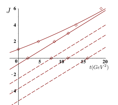
Figure 1: Positive C-parity glueball according to lattice gauge simulations Meyer:2004gx . The lines are our fit to Regge trajectories Shuryak:2013sra .

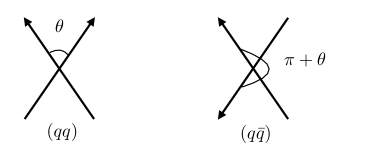
Figure 2: Euclidean rendering of the $qq$ scattering amplitude at relative angle $\theta$ and the $q\bar{q}$ scattering amplitude at angle $\theta+\pi$. The continuation to Minkowski space follows through $\theta\rightarrow-i\chi$ with the latter as the charge conjugate of the former. The relevance of this construction for the Pomeron and the Odderon is detailed in the text.

IV The phase of the Pomeron

Experimentally, the Pomeron scattering amplitude exibits both a real and imaginary part. The real part is measured at two locations: at small $t\approx 0$, by observing the interference with the weak Coulomb scattering, and at the location of the diffractive peak where the imaginary part vanishes. For the interference measurement, the results are expressed in terms of the so called $\rho$ parameter

$$\rho={{\rm Re}({\cal A}(s,t=0))\over{\rm Im}({\cal A}(s,t=0))}$$ (19)

The recent TOTEM data Antchev:2016vpy give

$$\rho(\sqrt{s}=8\,{\rm TeV})=0.12\pm 0.03$$ (20)

The textbook description of the Regge scattering amplitudes relates the $\rho-$parameter with the signature factor which for small $t$ is captured by the phase factor $e^{-\frac{i}{2}\pi\Delta_{\mathbb{P}}}$. It is small if $\Delta_{\mathbb{P}}$ is small, in agreement with data.

We now note how similar terms appear in the stringy amplitudes, starting from the positive definite charge signature $C=+1$, the Pomeron. Such a phase appears when analytically continuing the Euclidean scattering amplitude at angle $\theta$ to $\pi+\theta$ for the cross channel, as illustrated in Fig. 2 for quark-quark scattering. The result after integrating over the impact parameter and keeping only the two leading contributions in (14) is for the $C=+1$ signature

$${\cal A}^{+}(t,s)\approx 2is\left(\frac{\pi}{2}g_{s}a_{D}\right)^{2}$$

$$\left(\left({\rm ln}(s)\right)^{1-\frac{D_{\perp}}{2}}\,s^{\alpha_{\mathbb{P}}(t)}+\left({\rm ln}(-s)\right)^{1-\frac{D_{\perp}}{2}}\,(-s)^{\alpha_{\mathbb{P}}(t)}\right)$$

with $\alpha_{\mathbb{P}}(t)=\Delta+{\alpha^{\prime}_{\mathbb{P}}}t$. At large $\sqrt{s}$ and small $t$, (IV) is also characterized by an extra phase $e^{-\frac{i}{2}\pi\Delta}$ in agreement with textbooks. However, we note that while the pre-exponential factors with ${\rm ln}(s)$ disappear in 4-d flat space, i.e. $D_{\perp}=2$, as in the textbooks, they do not for $D_{\perp}>2$ as is the case of the holographic model (see (18)). The additional pre-exponential factors stem in this case from the diffusion in the additional holographic direction, and are thus completely necessary. Their inclusion through the branch ${\rm ln}(-s)\equiv{\rm ln}(s)+i\pi$ produces a correction to the phase which is asymptotically subleading at infinite $\chi$, but at current energies is about -15% (it enters with the opposite sign to the standard phase.) So, accurate measurements of the energy dependence of the phase can be sensitive to Gribov diffusion in the 5-th dimension.

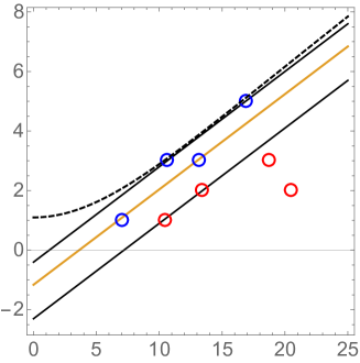
Figure 3: $C=-1$ parity glueballs on a Regge plot, showing their angular momentum $J$ versus their squared mass $M^{2}({\rm GeV})^{2}$. The two upper (blue) points and lines are for the negative spatial parity $P=-1$ gluballs, and the lower (red) ones are for the $P=+1$. The masses are from lattice gauge simulations Meyer:2004gx . The lines shows the hypothetical behavior of the Regge trajectories.

V The Odderon

Let us start with the phenomenology of glueballs. One can get some information about the odderon Regge trajectory following the same procedure as we used e.g. in Shuryak:2013sra . Specifically, this consists in: 1/ plotting the known masses (squared) of the appropriate glueballs; 2/ connecting those by plausible lines, to learn the relevant slope of the trajectories; 3/ extrapolating the upper trajectory to $t=0$. The corresponding plot for the masses of glueball with positive C parity, taken from the lattice study by Meyer Meyer:2004gx , is shown in Fig. 1 for completeness.

It is straightforward to extend it to glueballs with negative $C$-parity as well, as we show in Fig. 3. First, we note that there are 4 glueballs with negative $P=-1$ (vector-like) and 4 with positive $P=+1$ (axial-like) spatial parity. As seen from this figure, it appears that 6 of those 8 states make three pairs defining straight and parallel lines with the same (within errors) slope, namely $\alpha^{\prime}=0.32\,{\rm GeV}^{2}$. Furthermore, we note that the lowest (the leftest) vector $J^{PC}=1^{--}$ state seems to belong to the second trajectory. This feature is the same as for the positive $C$ parity case, in which the lowest scalar $0^{++}$ also belongs to the second trajectory. We take both features as indications that the trajectories are correct as drawn here.

Now, with only two states on the upmost trajectory, one can only define uniquely a straight line. Extrapolation of those to $t=0$ would indicate that the odderon intercept $\alpha_{\mathbb{O}}(0)$ is negative. If so, its contribution is suppressed by at least one power of $s$ compared to the Pomeron, or $\sqrt{s}$ compared to the mesonic Regge trajectories: in this case it is way too small to be observed at RHIC/Tevatron/LHC energies.

However, we know from experiment (the scattering data at negative $t$ for the Pomeron) as well as from the positive $C$-parity plot (in which one knows 3 states, $J=2,4,6$) that the upper Pomeron trajectory is not linear but curved. One may speculate that the same feature would hold for the odderon as illustrated by the speculative dashed line in Fig. 3.

On the theoretical side, the stringy description of the Pomeron also allows for a stringy odderon. The dipole-dipole scattering with negative signature follows the same reasoning as that for the positive signature in (IV), with now the result

$${\cal A}^{-}(t,s)\approx 2is\left(\frac{\pi}{2}g_{s}a_{D}\right)^{2}$$

$$\left(\left({\rm ln}(s)\right)^{1-\frac{D_{\perp}}{2}}\,s^{\alpha_{\mathbb{P}}(t)}-\left({\rm ln}(-s)\right)^{1-\frac{D_{\perp}}{2}}\,(-s)^{\alpha_{\mathbb{P}}(t)}\right)$$

At large $\sqrt{s}$ and small $t$, the amplitude (V) is only parametrically suppressed from (IV) by ${\rm tan}(\pi\Delta/2)$. Remarkably, for the critical bosonic string with $\Delta=D_{\perp}/12=2$, the odderon amplitude vanishes identically. This is not the case, for the holographic string with $2<D_{\perp}\leq 3$, where the suppression is parametrically small (especially for our empirical value of $\Delta_{\mathbb{P}}=0.18$), but with an odderon with the same intercept as the Pomeron. The inclusion of the higher stringy corrections should not alter qualitatively these observations.

Summarizing this section: the negative $C$-parity glueballs hint towards the existence of a set of Regge trajectories, with a slope different from any other set. If the leading trajectory is curved, the location of its intercept $\alpha_{O}(0)$ is likely to lie between zero and one. The odderon drops out from the critical bosonic string, but otherwise carries a similar intercept as the Pomeron for the non-critical and holographic string. While its relative contribution is small, its relyable observation would also be an indication to diffusion in the 5-th dimension.

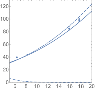
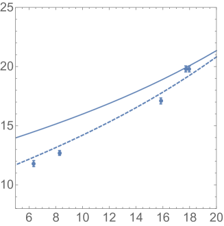
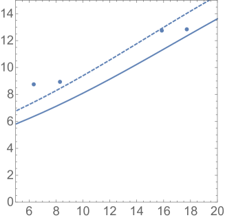
Figure 4: The upper plot shows $\sigma_{\rm tot}$ in $mb$ versus the log of the collision energy $\chi={\rm ln}(s/s_{0})$. The left-side (low energy) data points at $\sqrt{s}=27,63\,{\rm GeV}$ are from the old ISR measurements, and the three right-side points, for $\sqrt{s}=2.76,7,8\,{\rm TeV}$ are from the TOTEM measurements. The dotted line in the lower plot indicates the contribution of the Reggeons other than the Pomeron (from the PDG fit.) The middle plot shows the elastic slope $B$ (${\rm GeV}^{-2}$), and the lower plot is their ratio. The curves are for the profile shown in Fig. 5.

VI The Pomeron shape

VI.1 Phenomenology

The main information we have about the shape of the scattering amplitude $\Omega(s,b)$ can be summarized as follows. One observable is the total cross section, which is related to it via the optical theorem

$$\sigma_{\rm tot}=4\pi\int dbb\,{\rm Im}\,\left(\Omega(s,b)\right)$$ (23)

Some data points for the cross section are shown in the upper plot of Fig. 4. As well known, the cross section more than double from ISR to LHC energies. However, one should be aware that the low energy plots are affected by the Reggeons other than the Pomeron. Their contribution (from the PDG) is shown by the the dotted line in the left corner.

Another important parameter is the elastic slope $B$

$$B(t=0)=\left(-\frac{d{\rm ln}\sigma_{e}}{d|t|}\right)_{0}=\frac{1}{2}\left<b^{2}\right>_{\Omega}$$ (24)

The corresponding data are shown in the middle plot of Fig. 4. Their value also grows with the collision energy, which is due to the effective growth of the proton size induced by Gribov diffusion process.

In order to understand what these data tell us about the shape of the profile, it is useful also to plot their dimensionless ratio

$$R\equiv{\sigma_{\rm tot}(s)\over B(s)}$$ (25)

with the cross section expressed in ${\rm GeV}^{-2}$. This ratio is plotted in the lower plot in Fig. 4. In order to understand what the ratio (25) tells us, it is convenient to compare it to some simplified models for the shape, such as e.g. the black disc

$$\Omega_{bd}=\theta(b_{max}-b),\,\,\,R_{bd}=8\pi$$ (26)

the $Gaussian$ without a prefactor

$$\Omega_{G}=e^{-b^{2}/2b_{0}^{2}},\,\,\,R_{G}=4\pi$$ (27)

and the $exponential$, also without a prefactor

$$\Omega_{E}=e^{-b/b_{0}},\,\,\,R_{E}={4\pi\over 3}$$ (28)

The high energy values of the ratio are far from the two extreme shapes, and rather close to the Gaussian value. The low energy profiles are in fact also near-Gaussian, but with the prefactor smaller than one, as we will discuss below.

VI.2 The Pomeron shape and the mass of the string’s ends

As we already noted above, the shapes of the BFKL and BKYZ Pomeron scattering amplitudes $A(s,b)$ are both Gaussian, as is typical for diffusive processes. The prefactor, however, growing as $s^{\Delta}$, at high enough energy violates the unitarity.

A generic resolution for this situation is well known: one has to include the “multi-Pomeron effect”, see e.g. Schegelsky:2011aa and references therein. A standard procedure is Glauber unitarization, which follows from the substitution

$${\bf K}\rightarrow\Omega\equiv 1-e^{\bf-K}$$ (29)

The two leading terms in ${\bf K}$ compensate each other when

$$\chi\Delta\approx{b_{\rm black}^{2}\over 4\chi\alpha^{\prime}_{\mathbb{P}}}$$ (30)

For $b<b_{\rm black}$ the interaction is too strong, multiple Pomeron exchanges screen each other, and the proton is effectively black. Asymptotically, we have $b_{\rm black}\sim\chi^{2}$.

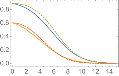
Figure 5: The unitarized profile function $\Omega=1-e^{\bf-K}$, for $\sqrt{s}=8000\,{\rm GeV}$ (upper blue curve) and $62\,{\rm GeV}$ (lower red curve), versus the impact parameter $b$ (${\rm GeV}^{-1}$). The solid curves at all plots are for the parameters $A=7.\,{\rm GeV}^{-2}$, $\mu=-0.04\,{\rm GeV}$, and the dashed ones are for $A=4.5\,{\rm GeV}^{-2}$, $\mu=0$. The dotted line in the lower plot indicate the contribution of the Reggeons other than the Pomeron.

The purpose of this subsection is to incorporate these effects, and also see whether the fit to the data may indicate a nonzero value of the first higher order term $\mu$. A technical point is that standard Reggeon expressions for the amplitude contains the nucleon form factors $f_{N}^{2}(t)$ times the Regge factor $s^{\alpha(t)}$. However, in order to perform unitarization (accounting for multi-Pomerons) one has to proceed to the coordinate profile, and in this case the product involves the convolution of functions, which is unnecessary complicated. A simple way out, sufficient for the purpose of this section, is to use Gaussian form factors $f_{N}^{2}(q)=e^{-Aq^{2}}$ which allows us to derive the coordinate profile analytically

$${\bf K}(s,b)=C\,{\rm exp}\left(\Delta_{\mathbb{P}}\chi-{b^{2}\over 4\left(A+\alpha^{\prime}_{\mathbb{P}}\chi\right)}+2\mu b\right)$$

where the normalization constant $C=2.2$ is fitted to the TOTEM data, as all higher order stringy contributions decreasing with $b$ are for now neglected. We remark that while the occurence of $A$ in (VI.2) is exact for one-Pomeron exchange, it is only an approximation in the unitarized multi-Pomeron resummation in the Glauber substitution (29).

A negative $\mu$ shifts the maximum of the profile function away from $b=0$, and modifies the shape in a way shown (for the unitarized profile functions) in Fig. 5. It turned out that the shape of the amplitude is sensitive to even small nonzero $\mu$.

Now we invite the reader to look at Fig. 4 again, now paying attention to the curves. In order to fit the upper plot, for the cross section, we used a smaller Pomeron intercept $\Delta=0.09$. The middle plot, for the elastic slope, is however independent of its value. One can see that the profile shape corresponding to $\mu=0$, the dashed line in the middle plot, describes the growth of $B(\chi)$ quite well (but is not good for the value of the ratio at the highest LHC point $\sqrt{s}=7\,TeV$ shown. The solid line is better on that. The fact that it misses the low energy points is less serious since one needs to subtract the non-Pomeron contributions. The upcoming LHC data for twice larger beam energy will clarify the situation, but for now we see that a small negative $\mu$ has a potential to make the description better. Perhaps the optimum, inside the simple ansatz for the shape we use, is somewhere in between these two curves.

The purpose of these comparisons is not to get an excellent fit to the data, as there are already several of those on the market, using multi-parameter and rather arbitrary functions. Our main message here is that the profile shape – and the two observables reflecting it – are very sensitive even to rather small $\mu$. We think this comparison tells us that its value is definitely small, perhaps slightly negative.

There are also some theoretical justifications for a nonzero $\mu$, with a suggested sign. In fact, we already mentioned it in (9): the extrinsic curvature term in the action does indeed produce such a contribution, see  Hidaka:2009xh ; Qian:2014jna . One may further ask if lattice studies of the potential can also help to find the magnitude of $\mu$. Unfortunately, on the lattice the constant term in the potential $\mu\sim 1/a$ is singular in the $a\rightarrow 0$ continuum limit (a pointlike charge). A subtraction is possible, but the accuracy of the remaining finite part is not good enough.

Concluding this section, let us also mention another (admittedly much more exotic) origin for the $B(s),\sigma(s)$ growth with energy: a hypothetical $repulsive$ string self-interaction, briefly discussed in Shuryak:2017phz .

VI.3 The Pomeron profile and the Hagedorn transition

In our paper Shuryak:2013sra we discussed the transition between the stringy and perturbative regime, using the so called Hagedorn transition in which strings get highly excited. At the beginning of this paper we have discussed the static potential, in which a specific structure – the “wiggle” indicating a transition between two regimes – has been identified. Furthermore, we argued that a stringy duality can connect the static potential and the scattering amplitude, in a well defined way.

Now, let us discuss the issue phenomenologically. Suppose a “wiggle” is also present in the Pomeron profile function: what observables should be used to locate it?

Our first comment is that $pp$ collisions at LHC energies already have a certain structure in its unitarized profile function, namely the black disc. Obviously any structure in the amplitude inside the black disc, for $r<r_{\rm bd}$, is unobservable. To go around this difficulty one can either return to much lower energies of $pp$ collisions, or focus on $\gamma p$ collisions at the future Electron-Ion Collider.

Suppose now that the “wiggle” happens at impact parameters $outside$ the black disc region. For simplicity, let us imagine a small peak in the profile function at certain value of the impact parameter $b_{\rm peak}>r_{\rm bd}$. A Fourier-Bessel transform to momentum space will produce an oscillating signal $\sim J_{0}(qb_{\rm peak})$. Its minimum is at $qb_{\rm peak}\approx 4$, and the second peak is at $qb_{\rm peak}\approx 7$, not far from $2\pi$.

In fact TOTEM at 8 TeV does observe certain non-Gaussian deviations of the elastic peak, parametrized by a simple Gaussian $e^{{\rm const}*t}$, with a minimum located at $q^{2}\approx 0.1\,{\rm GeV}^{2}$. If this corresponds to a structure in the profile function, its location should be at

$$b_{\rm peak}={4\over 0.316\,{\rm GeV}}\approx 2.5\,{\rm fm}$$ (32)

This distance is way too far for the location of the Hagedorn transition. The corresponding “tube” temperature is way too low, and cannot correpond to this transition.

VII Summary

The effective string theory suggests corrections to the fundamental string Lagrangian, and elucidates how these corrections modify the linearly rising potetial at shorter distances. QCD lattice numerical simulations do indeed reveal two universal “Luscher terms” and a new non-universal term at even shorter distances responsible for the appearance of a “wiggle” in the potential. Albeit small in amplitude, it clearly marks the transition from the perturbative to the stringy regime.

The description of the static heavy quark potential in QCD can be mapped onto the Pomeron scattering amplitude by string duality. We have suggested that the scattering amplitude can provide a more direct test of the string dynamics than the static potential. We have discussed the effects predicted by those approaches, for the Pomeron size and shape. The future experiments at the Electron-Ion Collider should allow, through the measurements of differential cross sections of $\gamma^{*}p$ scattering, to elucidate the structure of the Pomeron and more accurately define the domains of its pQCD and string descriptions.

Acknowledgements. We thank V.A.Petrov for useful comments on the first version of this manuscript. This work was supported by the U.S. Department of Energy under Contracts No. DE-FG-88ER40388 and DE-AC02-98CH10886.

VIII Appendix: Unitarization for fixed signature

The fully unitarized scattering amplitudes of given charge conjugation signature ${\cal T}^{C=\pm}$ in impact parameter space, follows from (13) in terms of ${\bf K}$, and its charge conjugate $\chi\rightarrow\chi-i\pi$ in terms of $\tilde{\bf K}$. Specifically, for fixed impact parameter we have

$${\cal T}^{+}+{\cal T}^{-}=2is\left(1-e^{-{\bf K}+\tilde{\bf K}}\right)$$

$${\cal T}^{+}-{\cal T}^{-}=2is\left(1-e^{-{\bf K}-\tilde{\bf K}}\right)$$ (33)

or equivalently

$${\cal T}^{+}=+2is\left(1-e^{-{\bf K}}{\rm cosh}\,\tilde{\bf K}\right)$$

$${\cal T}^{-}=-2is\,e^{-{\bf K}}\,{\rm sinh}\,\tilde{\bf K}$$ (34)

The total cross sections for $pp$ and $p\bar{p}$ scattering can be deduced from the forward scattering parts of (VIII)

$$\frac{1}{2}\left(\sigma_{p\bar{p}}+\sigma_{pp}\right)=\frac{4\pi}{s}\,{\rm Im}\,\tilde{\cal T}^{+}$$

$$\frac{1}{2}\left(\sigma_{p\bar{p}}-\sigma_{pp}\right)=\frac{4\pi}{s}\,{\rm Im}\,\tilde{\cal T}^{-}$$ (35)

where the Fourier transform at $t=0$ is subsumed in the amplitudes in (VIII).

References

- (1) V. N. Gribov, hep-ph/0006158; V. N. Gribov, ’Gauge Theories and Quark Confinement’, 2002, PHASIS.
- (2) E. A. Kuraev, L. N. Lipatov and V. S. Fadin, Sov. Phys. JETP 45, 199 (1977) [Zh. Eksp. Teor. Fiz. 72, 377 (1977)]; I. I. Balitsky and L. N. Lipatov, Sov. J. Nucl. Phys. 28, 822 (1978) [Yad. Fiz. 28, 1597 (1978)].
- (3) A. I. Shoshi, F. D. Steffen and H. J. Pirner, Nucl. Phys. A 709, 131 (2002) [hep-ph/0202012].
- (4) R. C. Brower, J. Polchinski, M. J. Strassler and C. -ITan, JHEP 0712, 005 (2007) [hep-th/0603115]. R. C. Brower, M. J. Strassler and C. -ITan, JHEP 0903, 092 (2009) [arXiv:0710.4378 [hep-th]].
- (5) G. Basar, D. E. Kharzeev, H. U. Yee and I. Zahed, Phys. Rev. D 85, 105005 (2012) [arXiv:1202.0831 [hep-th]].
- (6) E. Shuryak and I. Zahed, Phys. Rev. D 89, no. 9, 094001 (2014) [arXiv:1311.0836 [hep-ph]].
- (7) A. M. Polyakov, Nucl. Phys. B 268, 406 (1986); doi:10.1016/0550-3213(86)90162-8
- (8) M. Luscher, Nucl. Phys. B 180, 317 (1981); for a review see J. Greensite, Prog. Part. Nucl. Phys. 51, 1 (2003) [arXiv:hep-lat/0301023].
- (9) M. Luscher and P. Weisz, JHEP 0407, 014 (2004) [hep-th/0406205].
- (10) J. F. Arvis, Phys. Lett. 127B, 106 (1983).
- (11) O. Aharony and N. Klinghoffer, JHEP 1012, 058 (2010) [arXiv:1008.2648 [hep-th]].
- (12) Y. Hidaka and R. D. Pisarski, Phys. Rev. D 80, 074504 (2009) [arXiv:0907.4609 [hep-ph]].
- (13) Y. Qian and I. Zahed, Phys. Rev. D 92, no. 8, 085012 (2015) [arXiv:1410.1092 [nucl-th]].
- (14) In Qian:2014jna this shift effect was found to be suppressed as . The expansion used upsets the string duality enforced here.
- (15) V. A. Petrov and R. A. Ryutin, Mod. Phys. Lett. A 30, no. 18, 1550081 (2015) doi:10.1142/S0217732315500819 [arXiv:1409.8425 [hep-ph]].
- (16) B. B. Brandt, JHEP 1707, 008 (2017) doi:10.1007/JHEP07(2017)008 [arXiv:1705.03828 [hep-lat]].
- (17) E. Shuryak and I. Zahed, arXiv:1707.01885 [hep-ph].
- (18) A. Stoffers and I. Zahed, Phys. Rev. D 87, 075023 (2013) [arXiv:1205.3223 [hep-ph]].
- (19) J. P. Burq et al., Nucl. Phys. B 217, 285 (1983).
- (20) A. Donnachie and P. V. Landshoff, Phys. Lett. B 296, 227 (1992) [hep-ph/9209205].
- (21) H. B. Meyer, hep-lat/0508002.
- (22) G. Antchev et al. [TOTEM Collaboration], Eur. Phys. J. C 76, no. 12, 661 (2016) [arXiv:1610.00603 [nucl-ex]]; G. Antchev et al. [TOTEM Collaboration], Europhys. Lett. 101, 21002 (2013).
- (23) V. A. Schegelsky and M. G. Ryskin, Phys. Rev. D 85, 094024 (2012) [arXiv:1112.3243 [hep-ph]].