A Robust Solver for a Mixed Finite Element Method for the Cahn-Hilliard Equation

Abstract

We develop a robust solver for a mixed finite element convex splitting scheme for the Cahn-Hilliard equation. The key ingredient of the solver is a preconditioned minimal residual algorithm (with a multigrid preconditioner) whose performance is independent of the spacial mesh size and the time step size for a given interfacial width parameter. The dependence on the interfacial width parameter is also mild.

Keywords  Cahn-Hilliard equation; convex splitting; mixed finite element methods; MINRES; block diagonal preconditioner; multigrid.

1 Introduction

Let $\Omega\subset\mathbb{R}^{d}$, $d=2,3$, be an open polygonal or polyhedral domain, and consider the following form of the Cahn-Hilliard energy [7]:

$$E(\phi)=\int_{\Omega}\left(\frac{1}{4\varepsilon}(\phi^{2}-1)^{2}+\frac{\varepsilon}{2}|\nabla\phi|^{2}\right)d{x},$$ (1.1)

where $\varepsilon>0$ is a constant, and $\phi\in H^{1}(\Omega)$ represents a concentration field. The phase equilibria are represented by $\phi=\pm 1$ and the parameter $\varepsilon$ represents a non-dimensional interfacial width between the two phases.

The Cahn-Hilliard equation, which can be interpreted as the gradient flow of the energy (1.1) in the dual space of $H^{1}(\Omega)$, is often represented in mixed form by

$$\partial_{t}\phi=\varepsilon\Delta\mu, \text{in}\,\Omega,$$ (1.2a)

$$\mu=\varepsilon^{-1}\,\left(\phi^{3}-\phi\right)-\varepsilon\Delta\phi, \text{in}\,\Omega,$$ (1.2b)

together with the boundary conditions $\partial_{n}\phi=0$ and $\partial_{n}\mu=0$.

Let $T$ be a positive number and $H^{-1}_{N}(\Omega)$ be the dual space of $H^{1}(\Omega)$. A weak formulation of (1.2a)–(1.2b) is to find $(\phi,\mu)$ such that

$$\phi \in L^{\infty}\left(0,T;H^{1}(\Omega)\right)\cap L^{4}\left(0,T;L^{\infty}(\Omega)\right),$$ (1.3a)

$$\partial_{t}\phi \in L^{2}\bigl{(}0,T;H_{N}^{-1}(\Omega)\bigr{)},$$ (1.3b)

$$\mu \in L^{2}\bigl{(}0,T;H^{1}(\Omega)\bigr{)},$$ (1.3c)

and, for almost all $t\in(0,T)$,

$$\langle\partial_{t}\phi,\nu\rangle+\varepsilon\,a\!\left(\mu,\nu\right) =0\quad\forall\,\nu\in H^{1}(\Omega),$$ (1.4a)

$$\left(\mu,\psi\right)-\varepsilon\,a\!\left(\phi,\psi\right)-\varepsilon^{-1}\left(\phi^{3}-\phi,\psi\right) =0\quad\forall\,\psi\in H^{1}(\Omega).$$ (1.4b)

Here $\langle\cdot,\cdot\rangle$ denotes the duality pairing between the spaces $H^{-1}_{N}(\Omega)$ and $H^{1}(\Omega)$, $(\cdot,\cdot)$ is the inner product of $L^{2}(\Omega)$, and

$$a({u},{v})=(\nabla u,\nabla v).$$

The proof for the existence and uniqueness of the weak solution for (1.3)–(1.4) with initial data

$$\phi(0)=\phi_{0}\in\,H^{2}_{N}(\Omega)=\{v\in H^{2}(\Omega):\,\partial v/\partial n=0\;\text{on}\;\partial\Omega\}$$ (1.5)

can be found for example in [30].

The Cahn-Hilliard energy (1.1) along with the system (1.2) was originally developed to model phase separation of a binary fluid [7, 8, 15]. However, variations of the Cahn-Hilliard system are quickly becoming one of the most popular components in what are known as phase field models. The role that the Cahn-Hilliard equation takes in these models may best be described as creating an indicator function so that explicit tracking of the interface between two phases is not required. The growing number of applications include two phase flows, Hele-Shaw flows, copolymer fluids, crystal growth, void electromigration, vesicle membranes and more (cf. [18, 26, 10, 33, 3, 13] and the references therein).

There is a vast literature on numerical methods for the Cahn-Hilliard equation (cf. [31, 12, 25, 35, 37] and the references therein) and solvers based on various numerical schemes were developed in [2, 5, 9, 21, 22, 23, 29, 36, 28, 24, 35]. We will consider the mixed finite element method for (1.3)–(1.5) investigated in [11]. It is based on the convex splitting scheme in time [17] given by

$$\frac{\phi^{m}-\phi^{m-1}}{\tau}=\varepsilon\Delta\mu^{m},$$ (1.6a)

$$\Delta\mu^{m}=\frac{1}{\varepsilon}\left((\phi^{m})^{3}-\phi^{m-1}\right)-\varepsilon\Delta\phi^{m},$$ (1.6b)

where $\tau$ is the size of the time step, and a spatial discretization that employs Lagrange finite elements. This mixed finite element method is unconditionally stable and has optimal convergence in both time and space. Our goal is to develop a robust solver for this mixed finite element method.

The remainder of this paper is organized as follows. The mixed finite element method is introduced in Section 2, followed by the construction and analysis of the solver in Section 3. Numerical results that demonstrate the performance of the solver are presented in Section 4, and we end the paper with some concluding remarks in Section 5.

2 A Mixed Finite Element Method

Let $M$ be a positive integer, $0=t_{0}<t_{1}<\cdots<t_{M}=T$ be a uniform partition of $[0,T]$ and $\mathcal{T}_{h}$ be a quasi-uniform family of triangulations of $\Omega$ (cf. [6]). The Lagrange finite element space $S_{h}\subset H^{1}(\Omega)$ is given by

$$S_{h}=\{v\in C(\bar{\Omega}):\,v|_{K}\in{\mathcal{P}}_{1}(K)\,\forall\,\,K\in\mathcal{T}_{h}\},$$

and we define

$$\mathring{S}_{h}=S_{h}\cap L_{0}^{2}(\Omega),$$

where $L_{0}^{2}(\Omega)$ is the space of square integrable functions with zero mean.

The mixed finite element scheme for (1.6) investigated in [11] is defined as follows: For $1\leq m\leq M$, find $\phi_{h}^{m},\mu_{h}^{m}\in S_{h}$ such that

$$\left(\delta_{\tau}\phi_{h}^{m},\nu\right)+\varepsilon\,a\!\left(\mu_{h}^{m},\nu\right) =0\, \forall\,\nu\in S_{h},$$ (2.1a)

$$\left(\mu_{h}^{m},\psi\right)-\varepsilon^{-1}\,\big{(}{\left(\phi_{h}^{m}\right)^{3}-\phi_{h}^{m-1}},{\psi}\big{)}-\varepsilon\,a\!\left(\phi_{h}^{m},\psi\right) =0\, \forall\,\psi\in S_{h},$$ (2.1b)

$$\phi_{h}^{0}-R_{h}\phi_{0} =0.$$ (2.1c)

Here

$$\delta_{\tau}\phi_{h}^{m}=\frac{\phi_{h}^{m}-\phi_{h}^{m-1}}{\tau},$$

where $\tau=T/M$ is the size for the time step, and the Ritz projection operator $R_{h}:H^{1}(\Omega)\longrightarrow S_{h}$ is defined by

$$a(R_{h}v,w) =(v,w)\qquad\forall\,w\in S_{h},$$ (2.2a)

$$(R_{h}v-v,1) =0.$$ (2.2b)

Remark 2.1.

The energy law

$$E(\phi(t))+\int_{0}^{t}\varepsilon\left\|\nabla\mu(s)\right\|_{L^{2}(\Omega)}^{2}ds=E(\phi(0))\qquad\forall\,t\in[0,T]$$

is a key property of the solution of (1.3)–(1.5). It can be shown [11] that the solution of the finite element method defined by (2.1)–(2.2) also satisfies a similar energy law, which leads to $\phi_{h}\in L^{\infty}(0,T;L^{\infty}(\Omega))$ and $\mu_{h}\in L^{2}(0,T;L^{\infty}(\Omega))$. Moreover, under the assumption that $\phi\in H^{2}(0,T;L^{2}(\Omega))\cap L^{\infty}(0,T;W^{1,6}(\Omega))\cap H^{1}(0,T;H^{2}(\Omega)),\mu\in L^{\infty}(0,T;H^{1}(\Omega))\cap L^{2}(0,T;H^{2}(\Omega))$, and $0\leq\tau\leq\tau_{0}$ for a sufficiently small $\tau_{0}$, the error estimate

$$\max\limits_{1\leq m\leq M}\left\|\nabla\phi^{m}-\nabla\phi_{h}^{m}\right\|_{L^{2}}^{2}+\tau\sum_{m=1}^{M}\left\|\nabla\mu^{m}-\nabla\mu_{h}^{m}\right\|_{L^{2}}^{2}\leq C(\varepsilon,T)(\tau^{2}+h^{2})$$ (2.3)

holds for a positive constant $C$ that depends on $\varepsilon$ and $T$ but does not depend on $\tau$ and $h$.

It follows from (2.1) that $(\phi_{h}^{m},1)=(\phi_{0},1)$ for $0\leq m\leq M$, and hence

$$\phi_{h}^{m}=\overline{\phi}_{0}+\mathring{\phi}_{h}^{m}\quad\text{for}\quad 0\leq m\leq M,$$ (2.4)

where $\overline{\phi}_{0}={\left(\phi_{0},1\right)}/{\left(1,1\right)}$ is the mean of $\phi_{0}$ over $\Omega$ and $\mathring{\phi}_{h}\in\mathring{S}_{h}$. We can also write

$$\mu_{h}^{m}=\overline{\mu}_{h}^{m}+\mathring{\mu}_{h}^{m},$$ (2.5)

where $\overline{\mu}_{h}^{m}$ is a constant function and $\mathring{\mu}_{h}^{m}\in\mathring{S}_{h}$.

Using (2.4) and (2.5), we can rewrite (2.1a)–(2.1b) in the following equivalent form: For $1\leq m\leq M$, find $\mathring{\phi}_{h}^{m},\mathring{\mu}_{h}^{m}\in\mathring{S}_{h}$ such that

$$\big{(}{\delta_{\tau}\mathring{\phi}_{h}^{m}},{\nu}\big{)}+\varepsilon\,a\!\left(\mathring{\mu}_{h}^{m},\nu\right)=\, 0\, \forall\,\nu\in\mathring{S}_{h},$$ (2.6a)

$$({\mathring{\mu}_{h}^{m}},{\psi})-\varepsilon^{-1}\,\big{(}{(\mathring{\phi}_{h}^{m}+\overline{\phi}_{0})^{3}-\mathring{\phi}_{h}^{m-1}},{\psi}\big{)}-\varepsilon\,a({\mathring{\phi}_{h}^{m}},{\psi})=\, 0\, \forall\,\psi\in\mathring{S}_{h},$$ (2.6b)

where

$$\delta_{\tau}\mathring{\phi}_{h}^{m}=\frac{\mathring{\phi}_{h}^{m}-\mathring{\phi}_{h}^{m-1}}{\tau}.$$

Note that we can recover the constant function $\overline{\mu}_{h}^{m}$ from $\mathring{\phi}_{h}^{m}$ and $\mathring{\phi}_{h}^{m-1}$ through the relation

$$\left(\overline{\mu}_{h}^{m},1\right)=\varepsilon^{-1}\big{(}(\mathring{\phi}_{h}^{m}+\overline{\phi}_{0})^{3}-\mathring{\phi}_{h}^{m-1},{1}\big{)}$$

that follows from (2.1b), (2.4) and (2.5).

Remark 2.2.

The nonlinear system (2.6) defines the first order optimality condition at a minimum $\mathring{\phi}_{h}^{m}$ of the convex functional $\Phi:\mathring{S}_{h}\longrightarrow\mathbb{R}$ given by

$$\Phi_{h}(\varphi)=\frac{\varepsilon}{2\tau}a\!\left(\varrho,\varrho\right)+\frac{1}{4\varepsilon}\left\|\varphi+\overline{\phi}_{0}\right\|_{L^{4}}^{4}-\frac{1}{\varepsilon}\left(\mathring{\phi}_{h}^{m-1},\varphi\right)+\frac{\varepsilon}{2}a\!\left(\varphi,\varphi\right),$$

where $\varrho\in\mathring{S}_{h}$ is defined by

$$\varepsilon\,a\!\left(\varrho,\nu\right)+\left(\varphi-\mathring{\phi}_{h}^{m-1},\nu\right)=0\quad\forall\,\nu\in\mathring{S}_{h}.$$

Since this convex minimization problem has a unique minimum by the standard theory [14], the system (2.6) $($and hence (2.1)$)$ is also uniquely solvable.

3 A Robust Solver

We will solve the nonlinear system (2.6) by Newton’s iteration. Let $(\mathring{\phi}_{h,j}^{m},\mathring{\mu}_{h,j}^{m})\in\mathring{S}_{h}\times\mathring{S}_{h}$ be the output of the $j$-th step. In order to advance the iteration, we need to find $(\delta_{j}\mathring{\mu},\delta_{j}\mathring{\phi})\in\mathring{S}_{h}\times\mathring{S}_{h}$ such that

$$\tau\varepsilon\,a({\delta_{j}\mathring{\mu}},{\nu})+(\nu,\delta_{j}\mathring{\phi}) =F_{j}(\nu) \forall\,\nu\in\mathring{S}_{h},$$ (3.1a)

$$({\delta_{j}\mathring{\mu}},{\psi})-\left[3\varepsilon^{-1}\big{(}{(\phi_{h,j}^{m})^{2}\delta_{j}\mathring{\phi}},{\psi}\big{)}+\varepsilon\,a({\delta_{j}\mathring{\phi}},{\psi})\right] =G_{j}(\psi) \forall\,\phi\in\mathring{S}_{h},$$ (3.1b)

where $\phi_{h,j}^{m}=\mathring{\phi}_{h,j}^{m}+\overline{\phi}_{0}$ and

$$F_{j}(\nu) =\tau\varepsilon\,a({\mathring{\mu}_{h,j}^{m}},{\nu})+({\mathring{\phi}_{h,j}^{m}-\mathring{\phi}_{h,j}^{m-1}},{\nu}),$$ (3.2a)

$$G_{j}(\psi) =({\mathring{\mu}_{h,j}^{m}},{\psi})-\left[\varepsilon^{-1}\big{(}{(\phi_{h,j}^{m})^{3}-\mathring{\phi}_{h,j}^{m-1}},{\psi}\big{)}+\varepsilon\,a({\mathring{\phi}_{h,j}^{m}},{\psi})\right].$$ (3.2b)

The next output of the Newton iteration is then given by

$$(\mathring{\mu}_{h,j+1}^{m},\mathring{\phi}_{h,j+1}^{m})=(\mathring{\mu}_{h,j}^{m},\mathring{\phi}_{h,j}^{m})-(\delta_{j}\mathring{\mu},\delta_{j}\mathring{\phi}).$$ (3.3)

Below we will construct a robust solver for (3.1).

First we circumvent the inconvenient zero mean constraint by reformulating (3.1) as the following equivalent problem: Find $(\delta_{j}\mu,\delta_{j}\phi)\in S_{h}\times S_{h}$ such that

$$\tau\varepsilon\big{[}a\!\left(\delta_{j}\mu,\nu\right)+\left(\delta_{j}\mu,1\right)\left(\nu,1\right)\big{]}+\left(\nu,\delta_{j}\phi\right) =\tilde{F}_{j}(\nu) \forall\,\nu\in S_{h},$$ (3.4a)

$$\left(\delta_{j}\mu,\psi\right)-\left[3\varepsilon^{-1}\big{(}{(\phi^{m}_{h,j})^{2}\delta_{j}\phi},{\psi}\big{)}+\varepsilon\big{[}a({\delta_{j}\phi},{\psi})+\left(\delta_{j}\phi,1\right)\left(\psi,1\right)]\right] =\tilde{G}_{j}(\psi) \forall\,\psi\in S_{h},$$ (3.4b)

where

$$\tilde{F}_{j}(\nu)=\begin{cases}F_{j}(\nu)&\text{if }\nu\in\mathring{S}_{h}\\ 0&\text{if }\nu=1\end{cases}\quad\text{and}\quad\tilde{G}_{j}(\psi)=\begin{cases}G_{j}(\psi)&\text{if }\psi\in\mathring{S}_{h}\\ 0&\text{if }\psi=1\end{cases}.$$ (3.5)

Remark 3.1.

It is easy to check that both (3.1) and (3.4) are well-posed linear systems and that the solution $(\delta_{j}\mathring{\mu},\delta_{j}\mathring{\phi})$ of (3.1)–(3.2) also satisfies (3.4)–(3.5).

Under the change of variables

$$\left(\delta_{j}\mu,\nu\right)\rightarrow\tau^{-\frac{1}{4}}\varepsilon^{-\frac{1}{2}}\left(\delta_{j}\mu,\nu\right)\quad\text{and}\quad\left(\delta_{j}\phi,\psi\right)\rightarrow\tau^{\frac{1}{4}}\varepsilon^{\frac{1}{2}}\left(\delta_{j}\phi,\psi\right),$$

the system (3.4) becomes

$$\tau^{\frac{1}{2}}\left[a\!\left(\delta_{j}\mu,\nu\right)+({\delta_{j}\mu},{1})({\nu},{1})\right]+({\nu},{\delta_{j}\phi}) =\tilde{F}_{j}(\tau^{-\frac{1}{4}}\varepsilon^{-\frac{1}{2}}\nu),$$ (3.6a)

$$({\delta_{j}\mu},{\psi})-\big{[}3\tau^{\frac{1}{2}}\big{(}{(\phi^{m}_{h,j})^{2}\delta_{j}\phi},{\psi}\big{)}+\tau^{\frac{1}{2}}\varepsilon^{2}\left[a({\delta_{j}\phi},{\psi})+({\delta_{j}\phi},{1})({\psi},{1})\right]\big{]} =\tilde{G}_{j}(\tau^{\frac{1}{4}}\varepsilon^{\frac{1}{2}}\psi),$$ (3.6b)

for all $(\nu,\psi)\in S_{h}\times S_{h}$.

Let $n_{h}$ be the dimension of $S_{h}$ and $\varphi_{1},\ldots,\varphi_{n_{h}}$ be the standard nodal basis (hat) functions for $S_{h}$. The system matrix for (3.6) is given by

$$\begin{bmatrix}\tau^{\frac{1}{2}}\left({\bf K}+{\bf c}{\bf c}^{t}\right)&{\bf M}\\ {\bf M}&-\tau^{\frac{1}{2}}{\bf J}(\phi_{h,j}^{m})-\tau^{\frac{1}{2}}\varepsilon^{2}\left({\bf K}+{\bf c}{\bf c}^{t}\right)\end{bmatrix},$$ (3.7)

where the stiffness matrix $\bf K$ is defined by ${\bf K}(k,\ell)=(\nabla\varphi_{k},\nabla\varphi_{\ell})$, the mass matrix $\bf M$ is defined by ${\bf M}(k,\ell)=(\varphi_{k},\varphi_{\ell})$, the vector $\bf c$ is defined by ${\bf c}(k)=(\varphi_{k},1)$, and the matrix ${\bf J}(\phi_{h,j}^{m})$ is defined by

$${\bf J}(\phi_{h,j}^{m})(k,\ell)=3\big{(}(\phi^{m}_{h,j})^{2}\varphi_{k},\varphi_{\ell}\big{)}.$$

Note that, since the mixed finite element method is convergent, we can expect $(\phi^{m}_{h,j})^{2}$ to be close to 1 away from an interfacial region with width $\varepsilon$. Therefore, for small $\varepsilon$, we can take $(\phi^{m}_{h,j})^{2}$ to be 1 in the system matrix, i.e., we can replace ${\bf J}(\phi_{h,j}^{m})$ by $3{\bf M}$ in (3.7). The following result is motivated by this observation.

Theorem 3.2.

Let the matrices $\bf B$ and $\bf P$ be defined by

$${\bf B} =\begin{bmatrix}\tau^{\frac{1}{2}}({\bf K}+{\bf c}{\bf c}^{t})&{\bf M}\\ {\bf M}&-3\tau^{\frac{1}{2}}{\bf M}-\tau^{\frac{1}{2}}\varepsilon^{2}({\bf K}+{\bf c}{\bf c}^{t})\end{bmatrix},$$ (3.8)

$${\bf P} =\begin{bmatrix}\tau^{\frac{1}{2}}({\bf K}+{\bf c}{\bf c}^{t})+{\bf M}&{\bf 0}\\ {\bf 0}&\tau^{\frac{1}{2}}\varepsilon^{2}({\bf K}+{\bf c}{\bf c}^{t})+{\bf M}\end{bmatrix},$$ (3.9)

where $0\leq\tau,\varepsilon\leq 1$. There exist two positive constants $C_{1}$ and $C_{2}$ independent of $\varepsilon$, $h$ and $\tau$ such that

$$C_{2}\max(\tau^{\frac{1}{2}},\varepsilon)\leq|\lambda|\leq C_{1}\quad\text{\rm for any eigenvalue }\lambda\text{ of }{\bf P}^{-1}{\bf B}.$$ (3.10)

Proof.

A simple calculation shows that

$${\bf P}^{-1}{\bf B} =\left(\begin{bmatrix}{\bf M}&0\\ 0&{\bf M}\end{bmatrix}\begin{bmatrix}\tau^{\frac{1}{2}}\tilde{\bf K}+{\bf I}&0\\ 0&\tau^{\frac{1}{2}}\varepsilon^{2}\tilde{\bf K}+{\bf I}\end{bmatrix}\right)^{-1}\left(\begin{bmatrix}{\bf M}&0\\ 0&{\bf M}\end{bmatrix}\begin{bmatrix}\tau^{\frac{1}{2}}\tilde{\bf K}&{\bf I}\\ {\bf I}&-3\tau^{\frac{1}{2}}{\bf I}-\tau^{\frac{1}{2}}\varepsilon^{2}\tilde{\bf K}\end{bmatrix}\right)$$

$$=\begin{bmatrix}\tau^{\frac{1}{2}}\tilde{\bf K}+{\bf I}&0\\ 0&\tau^{\frac{1}{2}}\varepsilon^{2}\tilde{\bf K}+{\bf I}\end{bmatrix}^{-1}\begin{bmatrix}\tau^{\frac{1}{2}}\tilde{\bf K}&{\bf I}\\ {\bf I}&-3\tau^{\frac{1}{2}}{\bf I}-\tau^{\frac{1}{2}}\varepsilon^{2}\tilde{\bf K}\end{bmatrix},$$

where $\tilde{\bf K}={\bf M}^{-1}({\bf K}+{\bf c}{\bf c}^{t})$ and ${\bf I}$ is the $n_{h}\times n_{h}$ identity matrix.

By the spectral theorem, there exist ${\bf v}_{1},\ldots,{\bf v}_{n_{h}}\in\mathbb{R}^{n_{h}}$ and positive numbers $\kappa_{1},\ldots,\kappa_{n_{h}}$ such that

$$\tilde{\bf K}{\bf v}_{j}=\kappa_{j}{\bf v}_{j}\qquad\text{for}\quad 1\leq j\leq n_{h}$$

and

$${\bf v}_{j}^{t}{\bf M}{\bf v}_{\ell}=\begin{cases}1&\quad\text{if $j=\ell$}\\ 0&\quad\text{if $j\neq\ell$}\end{cases}\;.$$

Observe that the two dimensional space ${\bf V}_{j}$ spanned by

$$\begin{bmatrix}{\bf v}_{j}\\ 0\end{bmatrix}\quad\text{and}\quad\begin{bmatrix}0\\ {\bf v}_{j}\end{bmatrix}$$

is invariant under ${\bf P}^{-1}{\bf B}$ and

$${\bf P}^{-1}{\bf B}\left(\alpha\begin{bmatrix}{\bf v}_{j}\\ 0\end{bmatrix}+\beta\begin{bmatrix}0\\ {\bf v}_{j}\end{bmatrix}\right)=\gamma\begin{bmatrix}{\bf v}_{j}\\ 0\end{bmatrix}+\delta\begin{bmatrix}0\\ {\bf v}_{j}\end{bmatrix},$$

where

$$\begin{bmatrix}\gamma\\ \delta\end{bmatrix}=\begin{bmatrix}\tau^{\frac{1}{2}}\kappa_{j}+1&0\\ 0&\tau^{\frac{1}{2}}\varepsilon^{2}\kappa_{j}+1\end{bmatrix}^{-1}\begin{bmatrix}\tau^{\frac{1}{2}}\kappa_{j}&1\\ 1&-3\tau^{\frac{1}{2}}-\tau^{\frac{1}{2}}\varepsilon^{2}\kappa_{j}\end{bmatrix}\begin{bmatrix}\alpha\\ \beta\end{bmatrix}.$$

It follows that the eigenvalues of ${\bf P}^{-1}{\bf B}$ are precisely the eigenvalues of the matrix

$${\bf C}_{j} =\begin{bmatrix}\tau^{\frac{1}{2}}\kappa_{j}+1&0\\ 0&\tau^{\frac{1}{2}}\varepsilon^{2}\kappa_{j}+1\end{bmatrix}^{-1}\begin{bmatrix}\tau^{\frac{1}{2}}\kappa_{j}&1\\ 1&-3\tau^{\frac{1}{2}}-\tau^{\frac{1}{2}}\varepsilon^{2}\kappa_{j}\end{bmatrix}$$

$$=\begin{bmatrix}\displaystyle\frac{\tau^{\frac{1}{2}}\kappa_{j}}{\tau^{\frac{1}{2}}\kappa_{j}+1}&\displaystyle\frac{1}{\tau^{\frac{1}{2}}\kappa_{j}+1}\\[20.0pt] \displaystyle\frac{1}{\tau^{\frac{1}{2}}\varepsilon^{2}\kappa_{j}+1}&\displaystyle\frac{-3\tau^{\frac{1}{2}}-\tau^{\frac{1}{2}}\varepsilon^{2}\kappa_{j}}{\tau^{\frac{1}{2}}\varepsilon^{2}\kappa_{j}+1}\end{bmatrix}$$

for $1\leq j\leq n_{h}$. Hence we only need to understand the behavior of the eigenvalues of the matrix

$${\bf C}=\begin{bmatrix}\displaystyle\frac{\omega}{\omega+1}&\displaystyle\frac{1}{\omega+1}\\[20.0pt] \displaystyle\frac{1}{\omega\varepsilon^{2}+1}&\displaystyle\frac{-3\tau^{\frac{1}{2}}-\omega\varepsilon^{2}}{\omega\varepsilon^{2}+1}\end{bmatrix},$$

where $\omega$ is a positive number and $0<\tau,\varepsilon\leq 1$.

First of all we have

$$|\lambda|\leq\|{\bf C}\|_{\infty}\leq 4$$ (3.11)

for any eigenvalue $\lambda$ of ${\bf C}$, which implies that the second estimate in (3.10) holds for $C_{1}=4$.

A direct calculation shows that

$$|\det{\bf C}|=\frac{1+3\tau^{\frac{1}{2}}\omega+\varepsilon^{2}\omega^{2}}{1+(1+\varepsilon^{2})\omega+\varepsilon^{2}\omega^{2}}\geq\frac{1+3\tau^{\frac{1}{2}}\omega+\varepsilon^{2}\omega^{2}}{1+2\omega+\varepsilon^{2}\omega^{2}}.$$

On one hand we have

$$1+2\omega+\varepsilon^{2}\omega^{2}\leq\tau^{-\frac{1}{2}}(1+3\tau^{\frac{1}{2}}\omega+\varepsilon^{2}\omega^{2}),$$

which implies

$$|\det{\bf C}|\geq\tau^{\frac{1}{2}}.$$ (3.12)

On the other hand we also have

$$1+2\omega+\varepsilon^{2}\omega^{2}\leq\varepsilon^{-1}(1+2\varepsilon\omega+\varepsilon^{2}\omega^{2})\leq 2\varepsilon^{-1}(1+\varepsilon^{2}\omega^{2})\leq 2\varepsilon^{-1}(1+3\tau^{\frac{1}{2}}\omega+\varepsilon^{2}\omega^{2}),$$

which implies

$$|\det{\bf C}|\geq\frac{\varepsilon}{2}.$$ (3.13)

Putting (3.11)–(3.13) together we see that

$$4|\lambda|\geq|\det{\bf C}|\geq\max(\tau^{\frac{1}{2}},\varepsilon/2)$$

for any eigenvalue $\lambda$ of ${\bf C}$. Therefore the first estimate in (3.10) holds with $C_{2}=1/8$. ∎

In our numerical experiments we use the preconditioner ${\bf P}_{*}$ given by

$${\bf P}_{*}=\begin{bmatrix}\tau^{\frac{1}{2}}{\bf K}+{\bf M}&{\bf 0}\\ {\bf 0}&\tau^{\frac{1}{2}}\varepsilon^{2}{\bf K}+{\bf M}\end{bmatrix}.$$ (3.14)

Since the two symmetric positive definite matrices ${\bf P}$ and ${\bf P}_{*}$ are spectrally equivalent, we immediately deduce from Theorem 3.2 that there exist two positive constants $C_{3}$ and $C_{4}$ independent of $\varepsilon$, $h$ and $\tau$ such that

$$C_{4}\max(\tau^{\frac{1}{2}},\varepsilon)\leq|\lambda|\leq C_{3}$$ (3.15)

for any eigenvalue $\lambda$ of ${\bf P}_{*}^{-1}{\bf B}$.

According to (3.15), the performance of the preconditioned MINRES algorithm (cf. [19, 16]) for systems involving $\bf B$ is independent of $\tau$ and $h$ for a given $\varepsilon$, and also independent of $\varepsilon$ and $h$ for a given $\tau$. Similar behavior can also be expected for systems involving the matrix in (3.7). Furthermore, the action of $(\gamma{\bf K}+{\bf M})^{-1}$ on a vector can be computed by a multigrid method, which creates large computational savings.

Remark 3.3.

Recall the matrix ${\bf B}$ is obtained from the matrix in (3.7) by replacing ${\bf J}(\phi_{h,j}^{m})$ by $3{\bf M}$ and its justification depends on $\varepsilon$. Therefore we expect to see some dependence of the performance of the preconditioned MINRES algorithm on $\varepsilon$ for a given $\tau$.

Remark 3.4.

When $\tau$ becomes $0$, the matrix

$${\bf B}=\begin{bmatrix}0&{\bf M}\\ {\bf M}&0\end{bmatrix}$$

is well-conditioned. Therefore the performance of the preconditioned MINRES algorithm for systems involving the matrix in (3.7) will improve as the time step size decreases.

Remark 3.5.

Block diagonal preconditioners for saddle point systems are discussed in [4, 27] and the references therein.

4 Numerical Experiments

In this section we report the reulsts of eight numerical experiments in two and three dimensions. All computations were carried out using the FELICITY MATLAB/C++ Toolbox [34] unless specified otherwise.

In the first six numerical experiments, we solve (2.1) on the unit square $\Omega=(0,1)^{2}$ using uniform meshes. The initial mesh $\mathcal{T}_{0}$ is generated by the two diagonals of $\Omega$ and the meshes $\mathcal{T}_{1},\mathcal{T}_{2},\ldots$ are obtained from $\mathcal{T}_{0}$ by uniform refinements.

For the first five experiments, we use the initial data

$$\phi_{h}^{0}=\mathcal{I}_{h}\Big{[}\Big{(}\frac{1}{2}\Big{)}[1-\cos(2\pi x_{1})][1-\cos(2\pi x_{2}))]-1\Big{]},$$ (4.1)

where $\mathcal{I}_{h}:H^{2}(\Omega)\longrightarrow S_{h}$ is the standard nodal interpolation operator.

The system (2.1) (or equivalently (2.6)) is solved by the Newton iteration with a tolerance of $10^{-15}$ for $\|\delta_{j}\phi\|_{L^{\infty}(\Omega)}$ or a residual tolerance of $10^{-7}$ for (3.4)–(3.5), whichever is satisfied first. It turns out that only one Newton iteration is needed for each time step in all the experiments.

During each Newton iteration, the systems involving (3.7) are solved by a preconditioned MINRES algorithm with a residual tolerance of $10^{-7}$. The systems involving the preconditioner $\bf P$ are solved by a multigrid $V(4,4)$ algorithm that uses the Gauss-Seidel iteration as the smoother (cf. [20, 32]). In all our experiments the maximum number of preconditioned MINRES iterations occured during the first few time steps after which the number of iterations would decrease and level off.

In the first experiment, we take $\tau={0.002}/{64}$ with a final time $T=0.04$ for the two interfacial width parameters $\varepsilon=0.0625$ and $\varepsilon=0.001$. In Table 1 we report the average number of preconditioned MINRES iterations over all time steps along with the average solution time per time step as the mesh is refined. (The timing mechanism is the ‘tic toc’ command in MATLAB.) We observe that the performance of the preconditioned MINRES algorithm does not depend on $h$ and the solution time per time step grows linearly with the number of degrees of freedom. Moreover the solution time roughly doubles as $\varepsilon$ decreases from $0.0625$ to $0.001$, indicating that the performance of the solver only has a mild dependence on $\varepsilon$.

	$\varepsilon=0.0625$		$\varepsilon=0.001$
$h$	MINRES Its.	Time to Solve (s)	MINRES Its.	Time to Solve (s)
$\nicefrac{{\sqrt{2}}}{{8}}$	20	0.042391	28	0.01786
$\nicefrac{{\sqrt{2}}}{{16}}$	21	0.070047	44	0.04537
$\nicefrac{{\sqrt{2}}}{{32}}$	23	0.156576	57	0.13569
$\nicefrac{{\sqrt{2}}}{{64}}$	24	0.444770	71	0.50508
$\nicefrac{{\sqrt{2}}}{{128}}$	25	1.752561	107	3.13307
$\nicefrac{{\sqrt{2}}}{{256}}$	26	6.884936	96	12.3052
$\nicefrac{{\sqrt{2}}}{{512}}$	26	26.84091	97	57.2141
$\nicefrac{{\sqrt{2}}}{{1024}}$	26	108.9613	100	245.456

Table 1: The average number of preconditioned MINRES iterations over all time steps together with the average solution time per time step as the mesh is refined ($\Omega=(0,1)^{2},\tau=\nicefrac{{0.002}}{{64}}$, $T=0.04$ $\varepsilon=0.0625$ (left), $\varepsilon=0.001$ (right)).

Table 2 shows the average solution time per time step for the same problem with $\varepsilon=0.0625$ using FEniCS [1] on the prebuilt high-performance Docker. The main components of this code are Newton’s method and LU decomposition. The time step size is fixed at $\tau={0.002}/{64}$. The residual tolerance is set at $10^{-7}$. The timing mechanism is a start and stop of the python command ‘time.time’. By comparing Table 2 with Table 1, we see that FEniCS appears to be faster for the coarser mesh sizes. However, as the mesh is refined, the advantage of our method is clearly observed.

$h$	Avg. Time to Solve (s)
$\nicefrac{{\sqrt{2}}}{{8}}$	0.01449
$\nicefrac{{\sqrt{2}}}{{16}}$	0.02589
$\nicefrac{{\sqrt{2}}}{{32}}$	0.06675
$\nicefrac{{\sqrt{2}}}{{64}}$	0.21948
$\nicefrac{{\sqrt{2}}}{{128}}$	3.94694
$\nicefrac{{\sqrt{2}}}{{256}}$	44.4569

Table 2: The average solution time per time step using FEniCS to run the same test as performed in Table 1 with $\varepsilon=0.0625$

In the second experiment, we again take $\tau={0.002}/{64}$ and a final time $T=0.04$. The median numbers of the preconditioned MINRES iterations over all time steps for several values of $\varepsilon$ as the mesh is refined are plotted in Figure 1. The performance of our method is independent of the mesh size $h$, and there is some dependence on the interfacial width parameter $\varepsilon$ as expected (cf. Remark 3.3).

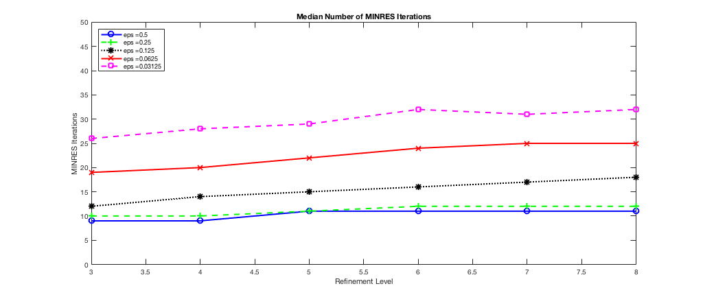
Figure 1: The median number of MINRES iterations over all time steps for several values of $\varepsilon$ as the mesh is refined ($\Omega=(0,1)^{2}$, $\tau=0.002/64$ and $T=0.04$).

In the third experiment, we fix $h=\sqrt{2}/64$, a final time $T=.04$, $\varepsilon=0.0625$ and $0.001$, and refine the time step size $\tau$. The average number of the preconditioned MINRES iterations over all time steps is displayed in Table 3 along with the average solution time per time step. The performance is clearly independent of the time step size $\tau$. The solution time roughly triples as $\varepsilon$ decreases from $0.0625$ to $0.001$, indicating again that the performance of the solver only depends mildly on $\varepsilon$.

	$\varepsilon=0.0625$		$\varepsilon=0.001$
$\tau$	MINRES Its.	Time to Solve (s)	MINRES Its.	Time to Solve (s)
$\nicefrac{{.002}}{{8}}$	27	0.310728	55	0.5297575
$\nicefrac{{.002}}{{16}}$	25	0.282849	57	0.5524107
$\nicefrac{{.002}}{{32}}$	25	0.273073	67	0.6346132
$\nicefrac{{.002}}{{64}}$	24	0.265608	71	0.6825223
$\nicefrac{{.002}}{{128}}$	23	0.260789	71	0.6788814
$\nicefrac{{.002}}{{256}}$	22	0.251007	78	0.7282336
$\nicefrac{{.002}}{{512}}$	20	0.237420	70	0.6503484
$\nicefrac{{.002}}{{1024}}$	18	0.219060	77	0.7032321

Table 3: The average number of preconditioned MINRES iterations over all time steps together with the average solution time per time step as the time step is refined ($\Omega=(0,1)^{2},h=\nicefrac{{\sqrt{2}}}{{64}}$, $T=0.04$, $\varepsilon=0.0625$ (left), $\varepsilon=0.001$ (right)).

In the fourth experiment, we fix $\varepsilon=0.0625$ and a final time $T=0.04$. The median numbers of preconditioned MINRES iterations over all time steps for several values of $\tau$ as the mesh is refined are displayed in Figure 2. The performance of our method is clearly independent of the mesh size $h$ and the time step size $\tau$.

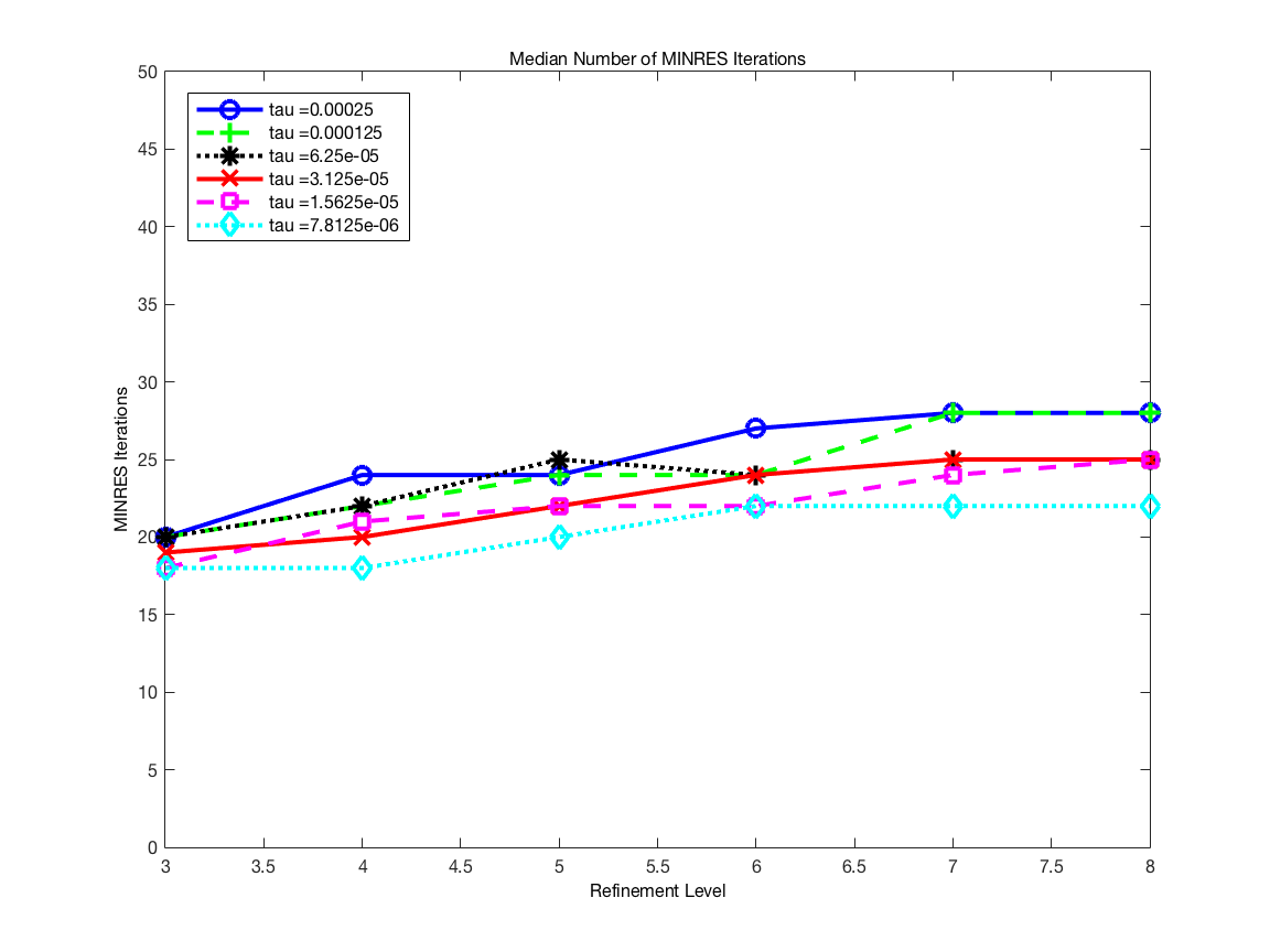
Figure 2: The median number of preconditioned MINRES iterations for several time step sizes as the mesh is refined ($\Omega=(0,1)^{2}$, $\varepsilon=0.0625$ and $T=0.04$).

In the fifth experiment, we fix the final time $T=0.04$ and let $\tau=0.002h/\sqrt{2}$ (cf. (2.3)). The median numbers of preconditioned MINRES iterations over all time steps for several values of $\varepsilon$ as the mesh is refined are displayed in Figure 3. Again, the performance only depends on the interfacial width parameter $\varepsilon$.

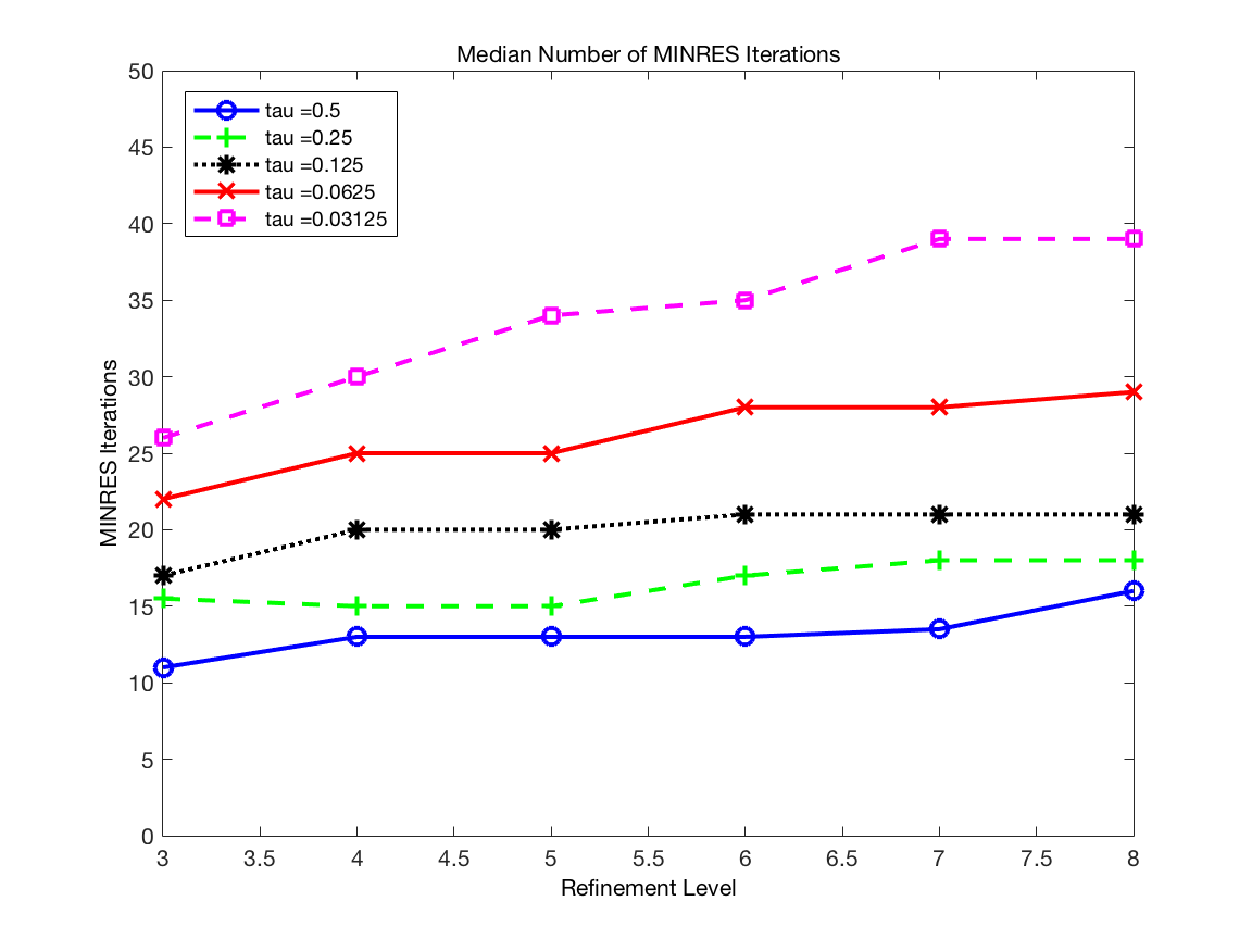
Figure 3: The median number of preconditioned MINRES iterations for several values of $\varepsilon$ as the mesh and time step are refined ($\Omega=(0,1)^{2}$, $\tau=0.002h/\sqrt{2}$ and $T=0.04$).

In the sixth experiment, we solve the Cahn-Hillard equation with a random initial condition. We take $h=\sqrt{2}/128$, $\tau=0.002/128$ and $\varepsilon=0.0625$. The surface plots for $\phi$ at $t=0$, $t=0.0025$, $t=0.005$, $t=0.0075$, $t=0.01$ and $t=0.0125$ are displayed in Figure 4. For comparison we solve the same problem using FEniCS and display the corresponding surface plots in Figure 5. The two figures are essentially indistinguishable.

(a)

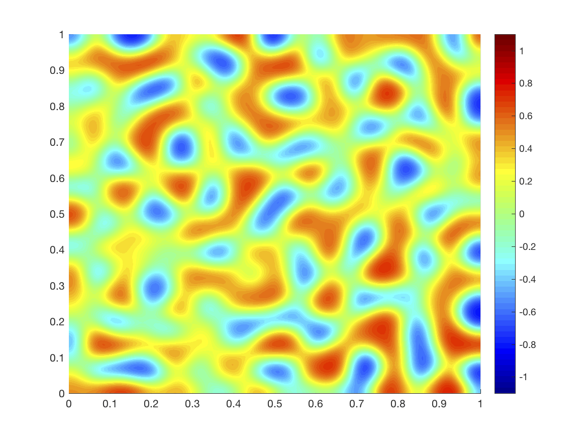
(b)

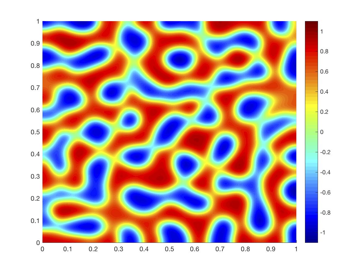
(c)

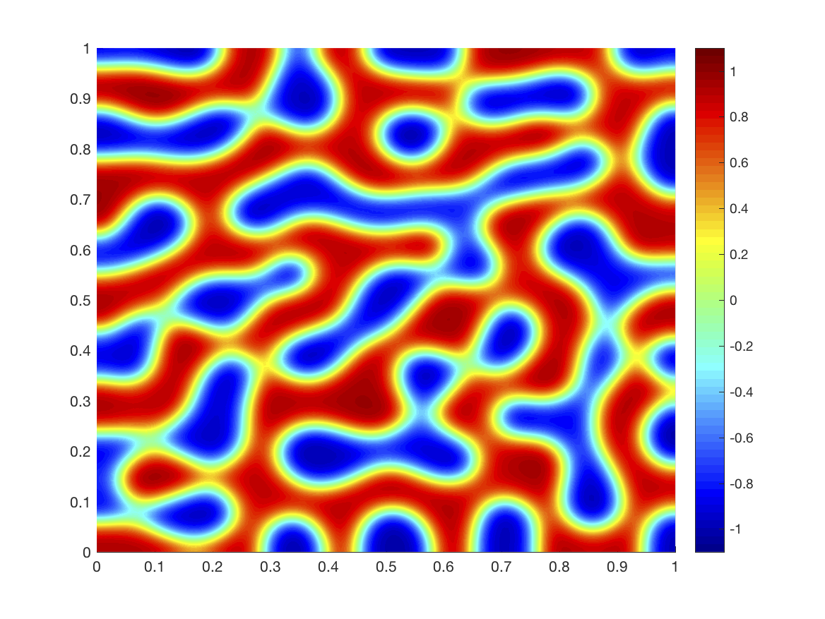
(d)

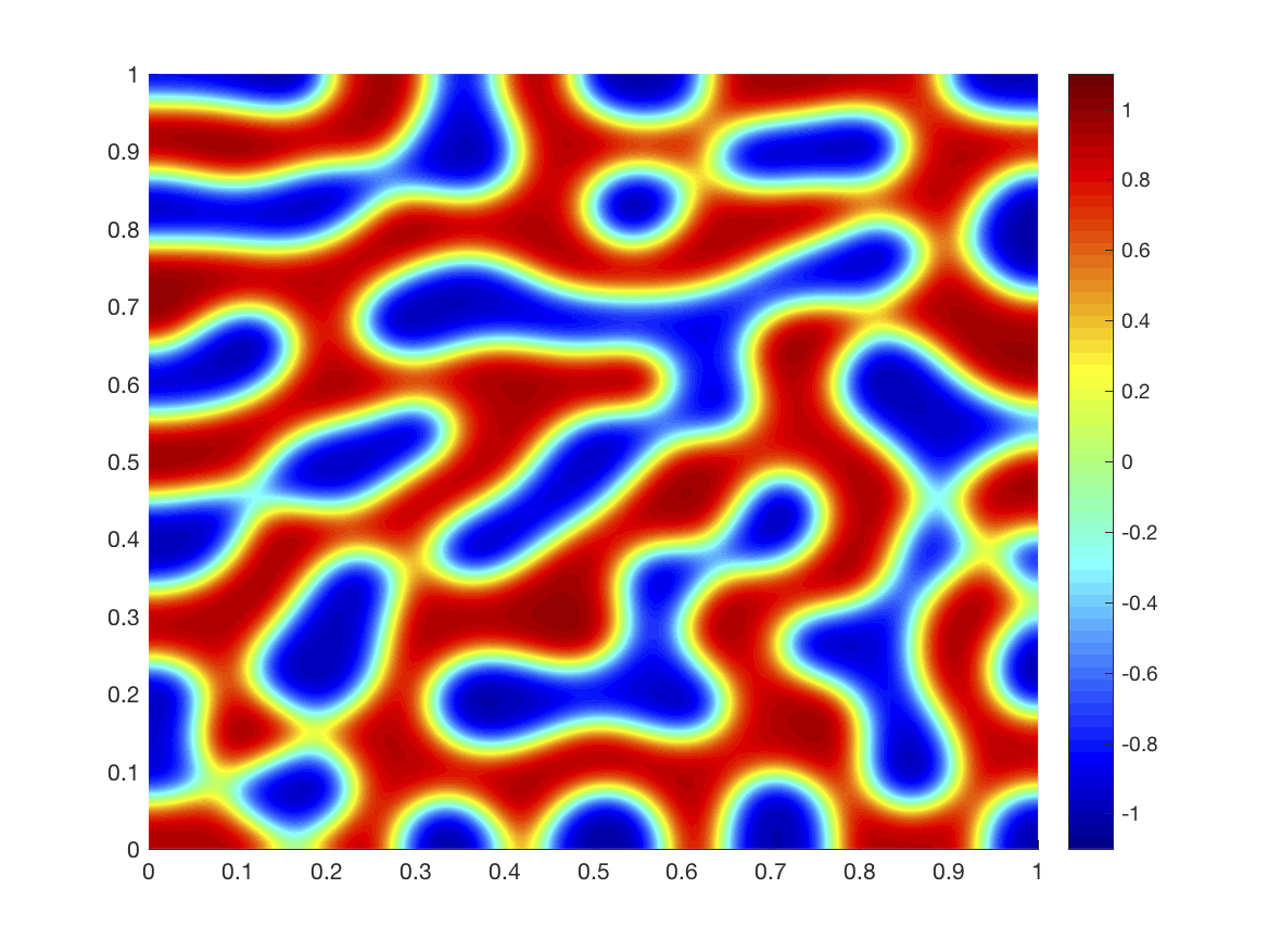
(e)

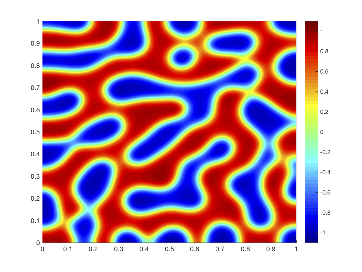
(f)

Figure 4: Spinodal decomposition of a binary fluid on $(0,1)^{2}$ with random initial data. The times displayed are $t=0,t=0.0025,t=0.005$ (top from left to right) and $t=0.0075,t=0.01,t=0.0125$ (bottom from left to right).

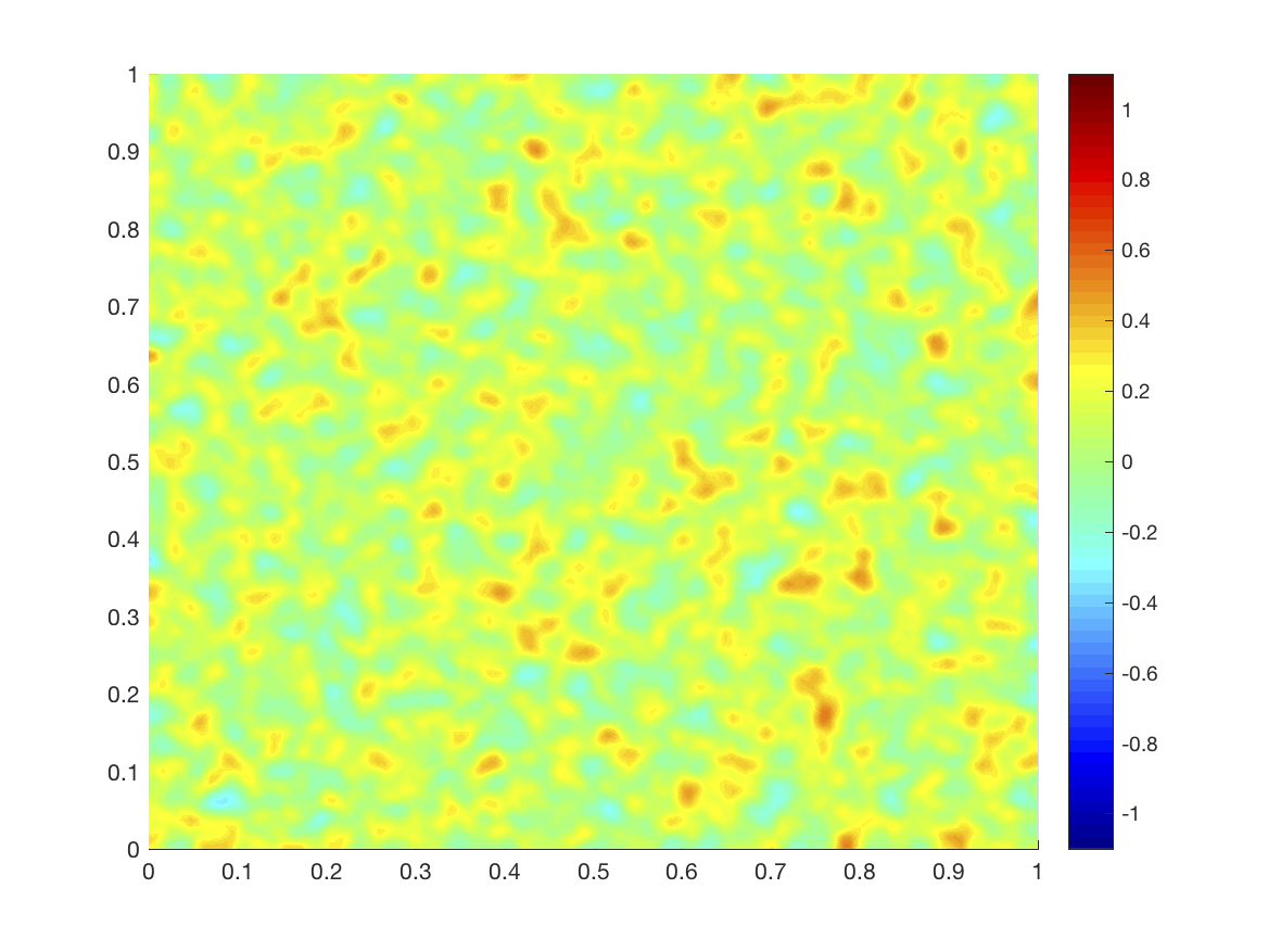
(a)

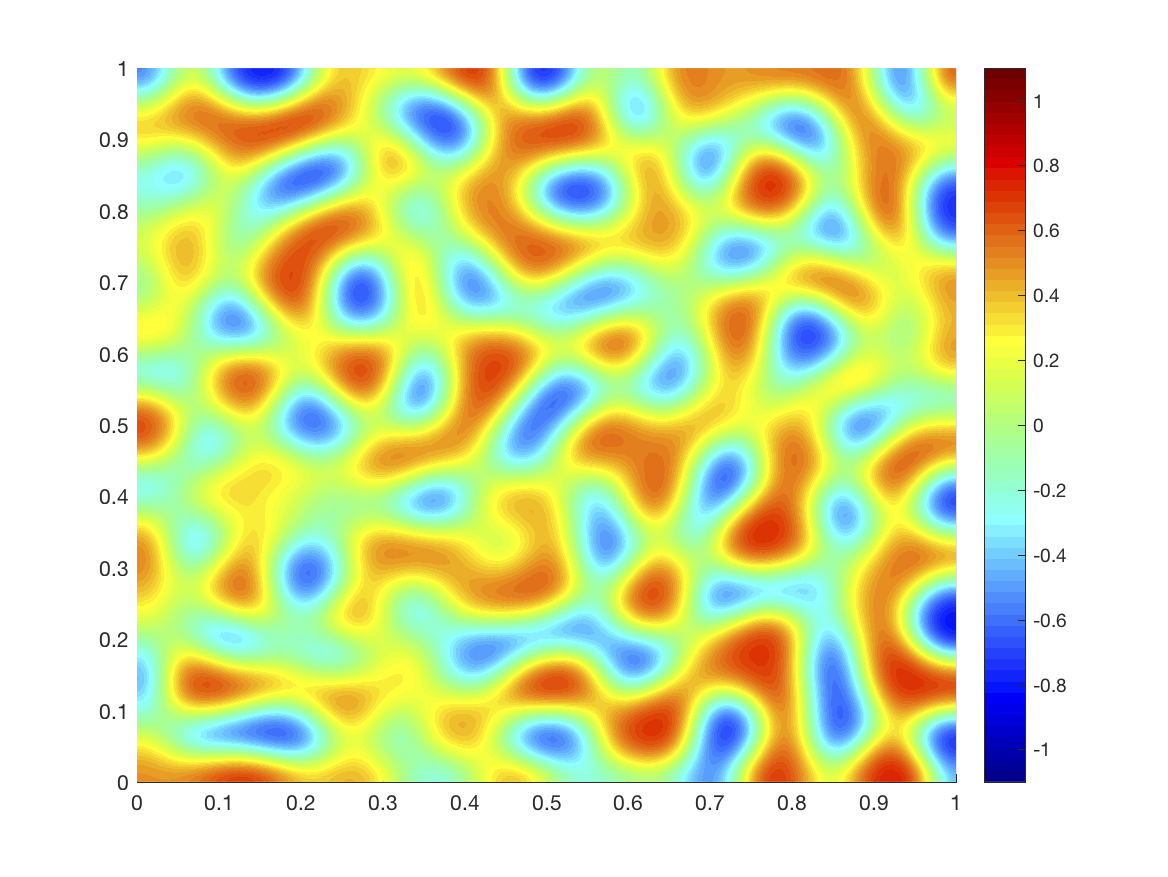
(b)

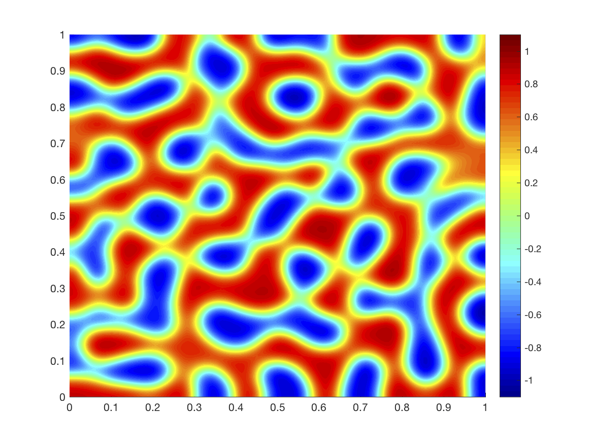
(c)

(d)

(e)

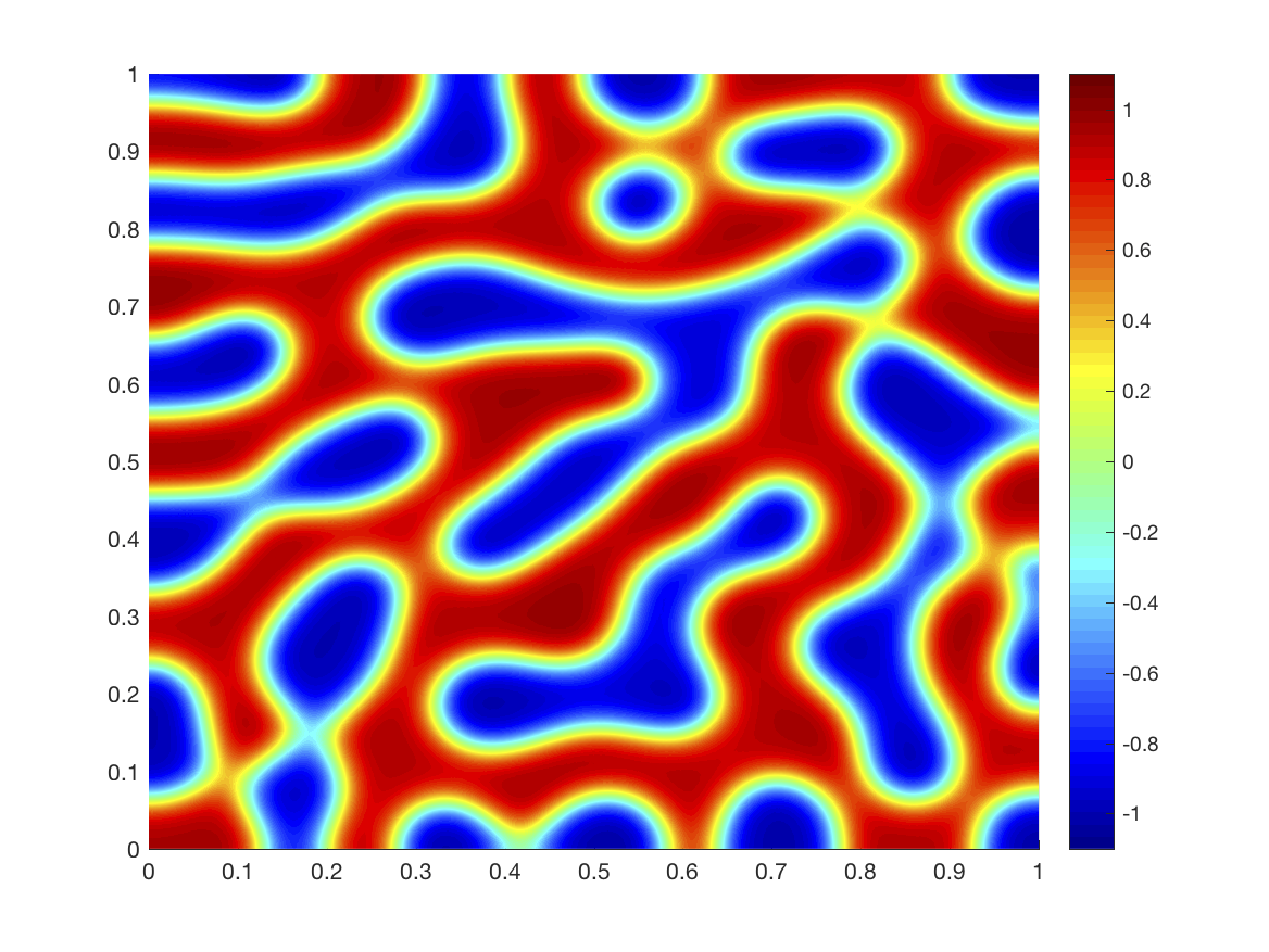
(f)

Figure 5: Spinodal decomposition of a binary fluid on $(0,1)^{2}$ with random initial data obtained by FEniCS. The times displayed are $t=0,t=0.0025,t=0.005$ (top from left to right) and $t=0.0075,t=0.01,t=0.0125$ (bottom from left to right).

In the seventh experiment, we solve the Cahn-Hilliard equation with a random initial condition on the unit cube $\Omega=(0,1)^{3}$ using uniform meshes. The initial mesh $\mathcal{T}_{0}$ consists of six tetrahedrons. The meshes $\mathcal{T}_{1},\mathcal{T}_{2},\cdots$ are obtained from $\mathcal{T}_{0}$ by uniform refinements. We take $\varepsilon=0.0625$, $\tau=0.002/64$, a final time $T=0.03$ and refine the mesh.

Table 4 displays the maximum, median, and average number of preconditioned MINRES iterations over all time steps along with the average solution time per time step. Again, only one Newton iteration is needed for each time step. We observe that the performance of the preconditioned MINRES algorithm does not depend on $h$ and the solution time per time step grows linearly with the number of degrees of freedom.

	MINRES Iterations			Time to Solve (s)
$h$	Max.	Med.	Avg.	Avg.
$\nicefrac{{\sqrt{3}}}{{8}}$	33	28	27	.0460738
$\nicefrac{{\sqrt{3}}}{{16}}$	33	29	29	.2451147
$\nicefrac{{\sqrt{3}}}{{32}}$	36	30	30	1.977465
$\nicefrac{{\sqrt{3}}}{{64}}$	37	29	30	15.97806
$\nicefrac{{\sqrt{3}}}{{128}}$	41	30	31	169.7146

Table 4: The maximum, median and average number of preconditioned MINRES iterations over all time steps together with the average solution time per time step as the mesh is refined ($\Omega=(0,1)^{3}$, $\varepsilon=0.0625$, $\tau=0.002/64$ and $T=0.03$).

Isocap plots for $\phi$ at $t=0,t=0.0015625,t=0.003125,t=0.0046875$, $t=0.00625$ and $t=0.0078125$ are displayed in Figure 6.

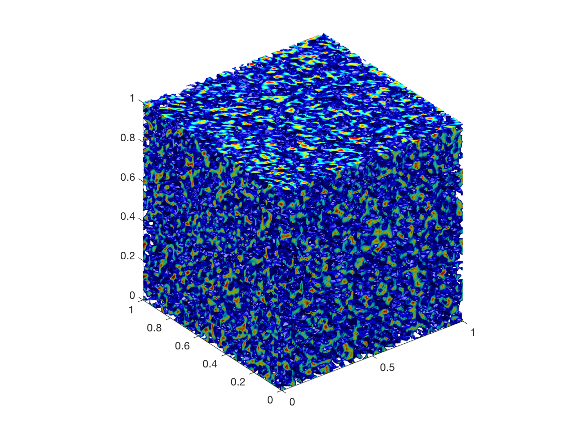
(a)

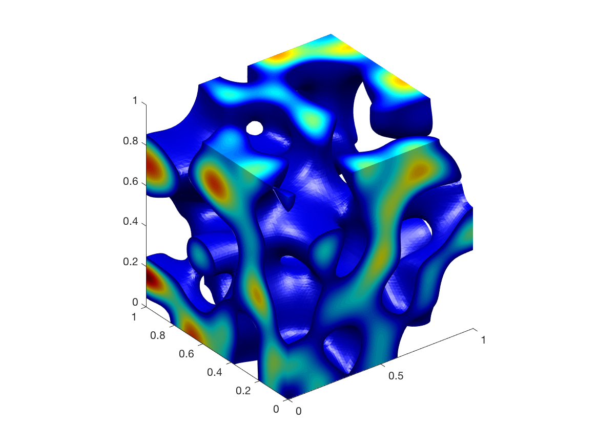
(b)

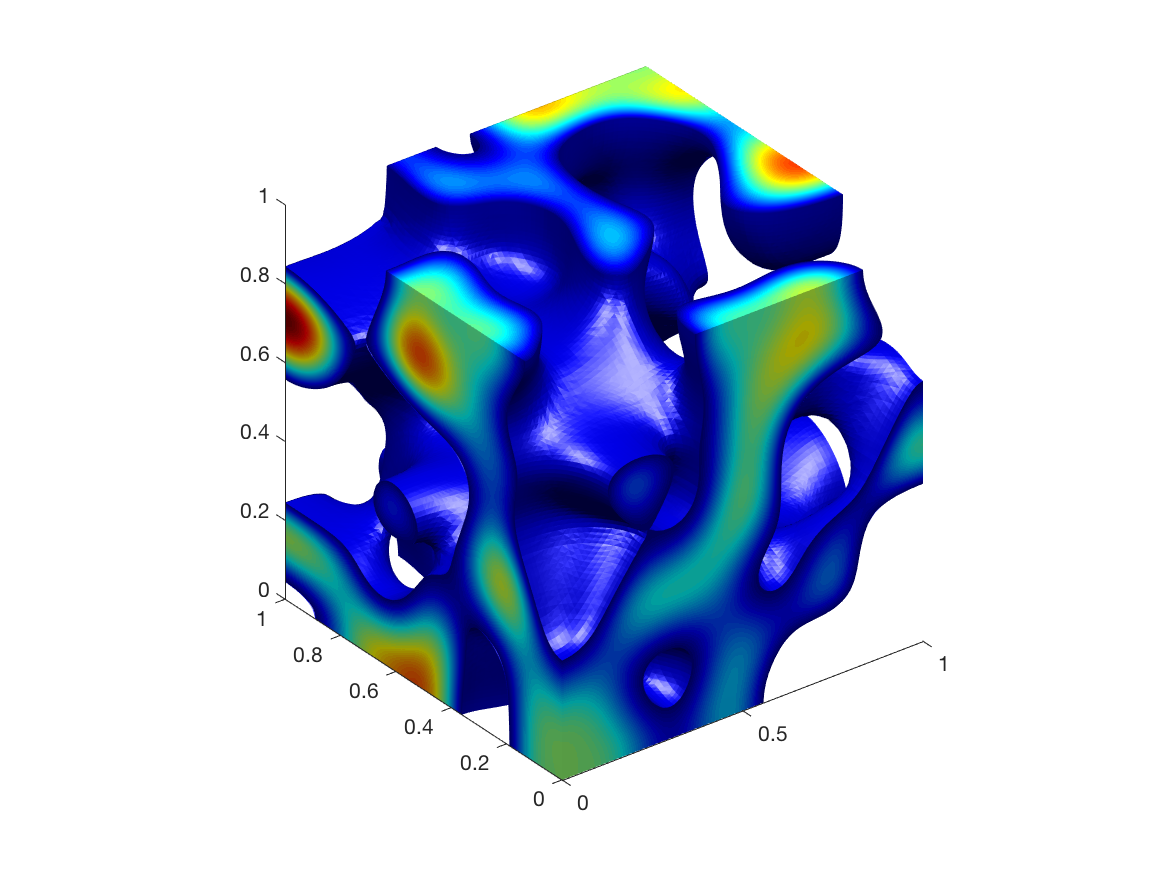
(c)

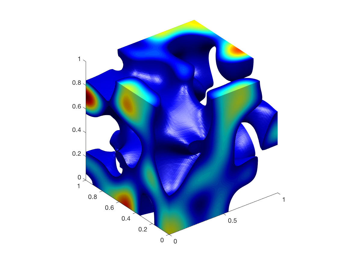
(d)

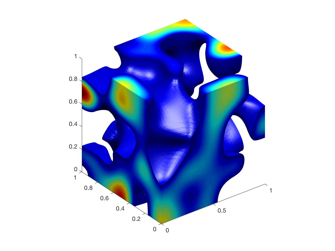
(e)

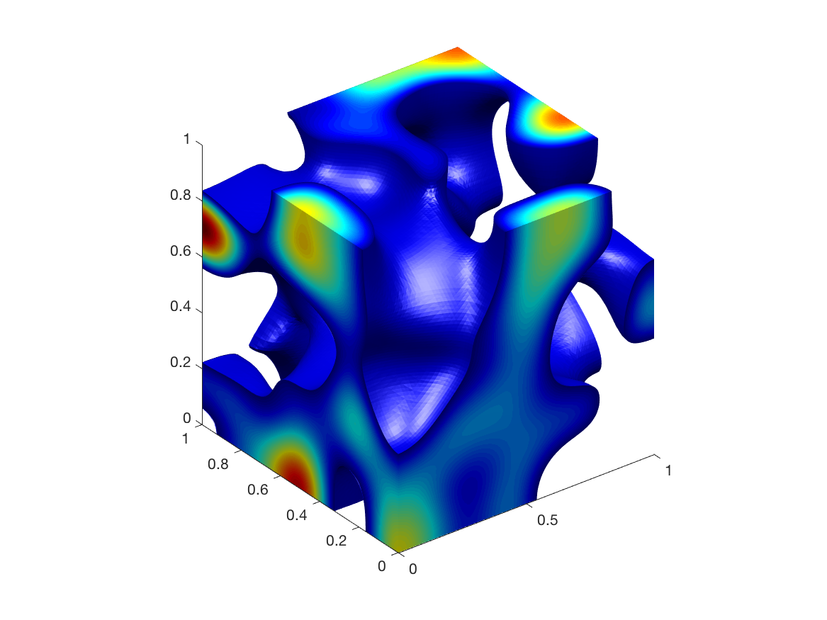
(f)

Figure 6: Spinodal decomposition of a binary fluid on $(0,1)^{3}$. The times displayed are $t=0,t=0.0015625,t=0.003125$ (top from left to right) and $t=0.0046875,t=0.00625,t=0.0078125$ (bottom from left to right).

In the eighth experiment, we solve the Cahn-Hilliard equation with a random initial condition. We take $h=\nicefrac{{\sqrt{3}}}{{32}},\tau=\nicefrac{{0.002}}{{64}}$ and $\varepsilon=0.0625$. Isocap plots for $t=0,t=0.015$ and $t=0.03$ are displayed in Figure 7. For comparison, we solve the same problem using FEniCS and display the corresponding isocap plots in Figure 8. The two figures are, again, essentially indistinguishable. Furthermore, we achieve considerable savings in time by using our solver. Specifically, the test using our solver completed in under 30 minutes whereas the test using FEniCS required 24 hours to reach the same final stopping time of $T=0.03$.

(a)

(b)

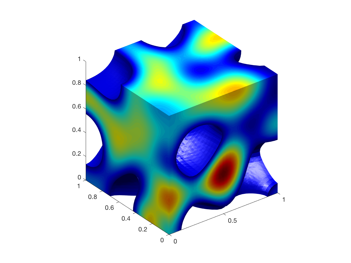
(c)

Figure 7: Spinodal decomposition of a binary fluid on $(0,1)^{3}$ with random initial data. The times displayed are $t=0,t=0.015,t=0.03$ (from left to right).

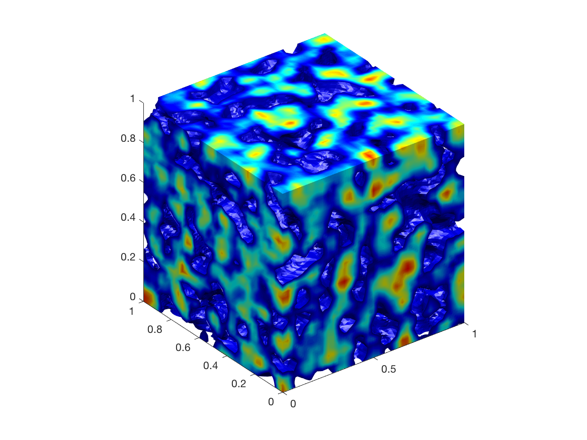
(a)

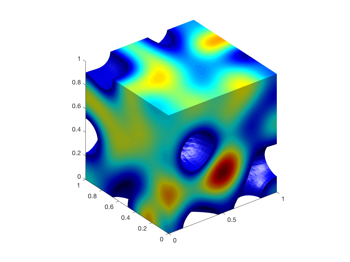
(b)

(c)

Figure 8: Spinodal decomposition of a binary fluid on $(0,1)^{3}$ with random initial data using FEniCS. The times displayed are $t=0,t=0.015,t=0.03$ (from left to right).

5 Concluding Remarks

We have developed a robust solver for a mixed finite element convex splitting scheme for the Cahn-Hilliard equation, where in each time step the Jacobian system for the Newton iteration is solved by a preconditioned MINRES algorithm with a block diagonal multigrid preconditioner. The robustness of our solver is confirmed by numerical tests in two and three dimensions. We have also validated our numerical results through comparisons with the results obtained through FEniCS and observed significant speed-up.

The methodology developed in this paper can be adapted for coupled systems that involve the Cahn-Hilliard equation, such as the Cahn-Hilliard Navier Stokes system (cf. [31] and the references therein). This is the topic for an ongoing research project.

References

[1]
M. S. Alnæs, J. Blechta, J. Hake, A. Johansson, B. Kehlet, A. Logg,
C. Richardson, J. Ring, E. Rognes M, and G. N. Wells.
The fenics project version 1.5.
Archive of Numerical Software, 3, 2015.
[2]
O. Axelsson, P. Boyanova, M. Kronbichler, M. Neytcheva, and X. Wu.
Numerical and computational efficiency of solvers for two-phase
problems.
Comput. Math. Appl., 65:301–314, 2013.
[3]
J.W. Barrett, R. Nurnberg, and V. Styles.
Finite element approximation of a phase field model for void
electromigration.
SIAM J. Numer. Anal., 42(2):738–772, 2005.
[4]
M. Benzi, G.H. Golub, and J. Liesen.
Numerical solution of saddle point problems.
Acta Numerica, 14:1–137, 2005.
[5]
P. Boyanova, M. Do-Quang, and M. Neytcheva.
Efficient preconditioners for large scale binary Cahn-Hilliard
models.
Comput. Methods Appl. Math., 12(1):1–22, 2012.
[6]
S.C. Brenner and L.R. Scott.
The Mathematical Theory of Finite Element Methods Third
Edition.
Springer-Verlag, New York, 2008.
[7]
J.W. Cahn.
On spinodal decomposition.
Acta Metall., 9:795, 1961.
[8]
J.W. Cahn and J.E. Hilliard.
Free energy of a nonuniform system. I. interfacial free energy.
J. Chem. Phys., 28:258, 1958.
[9]
H. D. Ceniceros and A. M. Roma.
A nonstiff, adaptive mesh refinement-based method for the
Cahn–Hilliard equation.
J. Comput. Phys., 225:1849–1862, 2007.
[10]
R. Choksi, M. Maras, and J. F. Williams.
2d phase diagram for minimizers of a Cahn-Hilliard functional with
long-range interactions.
SIAM J. Appl. Dyn. Sys., 10(4):1344–1362, 2011.
[11]
A. Diegel, X. Feng, and S. M. Wise.
Analysis of a mixed finite element method for a
Cahn-Hilliard-Darcy-Stokes system.
SIAM J. Numer. Anal., 53(1):127–152, 2015.
[12]
A. Diegel, C. Wang, and S. M. Wise.
Stability and convergence of a second-order mixed finite element
method for the Cahn-Hilliard equation.
IMA J. Numer. Anal., 36:1867–1897, 2016.
[13]
Q. Du, M. Li, and C. Liu.
Analysis of a phase field Navier-Stokes vesicle-fluid interaction
model.
Discrete Contin. Dyn. Syst. Ser. B, 8(3):539, 2007.
[14]
I. Ekeland and R. Témam.
Convex Analysis and Variational Problems.
Classics in Applied Mathematics. Society for Industrial and Applied
Mathematics (SIAM), Philadelphia, PA, 1999.
[15]
C.M. Elliott and S. Zheng.
On the Cahn-Hilliard equation.
Arch. Ration. Mech. Anal., 96:339–357, 1986.
[16]
H.C. Elman, D.J. Silvester, and A.J. Wathen.
Finite Elements and Fast Iterative Solvers: with Applications
in Incompressible Fluid Dynamics.
Oxford University Press, Oxford, second edition, 2014.
[17]
D. Eyre.
Unconditionally Gradient Stable Time Marching the Cahn-Hilliard
Equation.
In J W Bullard, R Kalia, M Stoneham, and L Q Chen, editors, Computational and Mathematical Models of Microstructural Evolution,
volume 53, pages 1686–1712, Warrendale, PA, USA, 1998. Materials Research
Society.
[18]
X. Feng.
Fully discrete finite element approximations of the
Navier-Stokes-Cahn-Hilliard diffuse interface model for two-phase fluid
flows.
SIAM J. Numer. Anal., 44:1049–1072, 2006.
[19]
A. Greenbaum.
Iterative Methods for Solving Linear Systems.
SIAM, Philadelphia, 1997.
[20]
W. Hackbusch.
Multi-grid Methods and Applications.
Springer-Verlag, Berlin-Heidelberg-New York-Tokyo, 1985.
[21]
D. Kay and R. Welford.
A multigrid finite element solver for the Cahn–Hilliard equation.
J. Comput. Phys., 212:288–304, 2006.
[22]
J. Kim.
A numerical method for the Cahn–Hilliard equation with a variable
mobility.
Commun. Nonlinear Sci. Numer. Simul., 12:1560–1571, 2007.
[23]
J. Kim, K. Kang, and J. Lowengrub.
Conservative multigrid methods for Cahn-Hilliard fluids.
J. Comput. Phys., 193:511–543, 2004.
[24]
C. Lee, D. Jeong, J. Shin, Y. Li, and J. Kim.
A fourth-order spatial accurate and practically stable compact scheme
for the Cahn–Hilliard equation.
Physica A, 409:17–28, 2014.
[25]
D. Lee, J. Huh, D. Jeong, J. Shin, A. Yun, and J. Kim.
Physical, mathematical, and numerical derivations of the
Cahn–Hilliard equation.
Comp Mater Sci, 81:216–225, 2014.
[26]
H. G. Lee, J. S. Lowengrub, and J. Goodman.
Modeling pinchoff and reconnection in a Hele-Shaw cell. I. the
models and their calibration.
Phys. Fluids, 14:492–513, 2002.
[27]
K.-A. Mardal and R. Winther.
Preconditioning discretizations of systems of partial differential
equations.
Numer. Linear Algebra Appl., 18:1–40, 2011.
[28]
J. Shin, S. Kim, D. Lee, and J. Kim.
A parallel multigrid method of the Cahn–Hilliard equation.
Comp Mater Sci, 71:89–96, 2013.
[29]
R. H. Stogner, G. F. Carey, and B. T. Murray.
Approximation of Cahn–Hilliard diffuse interface models using
parallel adaptive mesh refinement and coarsening with C1 elements.
Internat. J. Numer. Methods Engrg., 76:636–661, 2008.
[30]
R. Temam.
Infinite-Dimensional Dynamical Systems in Mechanics and
Physics.
Springer-Verlag, New York, 1988.
[31]
G Tierra and F Guillén-González.
Numerical methods for solving the Cahn–Hilliard equation and its
applicability to related energy-based models.
Arch Comput Method E, 22:269–289, 2015.
[32]
U. Trottenberg, C. Oosterlee, and A. Schüller.
Multigrid.
Academic Press, San Diego, 2001.
[33]
S. van Teeffelen, R. Backofen, A. Voigt, and H. Löwen.
Derivation of the phase-field-crystal model for colloidal
solidification.
Phys. Rev. E, 79:051404, 2009.
[34]
S.W. Walker.
FELICITY: Finite ELement Implementation and Computational
Interface Tool for You.
http://www.mathworks.com/matlabcentral/fileexchange/31141-felicity.
[35]
W. Wang, L. Chen, and J. Zhou.
Postprocessing mixed finite element methods for solving
Cahn–Hilliard equation: Methods and error analysis.
J Sci Comput, 67:724–746, 2016.
[36]
S.M. Wise.
Unconditionally stable finite difference, nonlinear multigrid
simulation of the Cahn-Hilliard-Hele-Shaw system of equations.
J. Sci. Comput., 44:38–68, 2010.
[37]
J. Zhou, L. Chen, Y. Huang, and W. Wang.
An efficient two-grid scheme for the Cahn-Hilliard equation.
Commun Comput Phys, 17:127–145, 2015.