HST Grism Observations of a Gravitationally Lensed Redshift 9.5 Galaxy

Abstract

We present deep spectroscopic observations of a Lyman-break galaxy candidate (hereafter MACS1149-JD) at $z\sim 9.5$ with the Hubble Space Telescope (HST) WFC3/IR grisms. The grism observations were taken at 4 distinct position angles, totaling 34 orbits with the G141 grism, although only 19 of the orbits are relatively uncontaminated along the trace of MACS1149-JD. We fit a 3-parameter ($z$, F160W mag, and Ly$\alpha$ equivalent width) Lyman-break galaxy template to the three least contaminated grism position angles using an MCMC approach. The grism data alone are best fit with a redshift of $z_{\mathrm{grism}}=9.53^{+0.39}_{-0.60}$ (68% confidence), in good agreement with our photometric estimate of $z_{\mathrm{phot}}=9.51^{+0.06}_{-0.12}$ (68% confidence). Our analysis rules out Lyman-alpha emission from MACS1149-JD above a $3\sigma$ equivalent width of 21 Å, consistent with a highly neutral IGM. We explore a scenario where the red Spitzer/IRAC $[3.6]-[4.5]$ color of the galaxy previously pointed out in the literature is due to strong rest-frame optical emission lines from a very young stellar population rather than a 4000 Å break. We find that while this can provide an explanation for the observed IRAC color, it requires a lower redshift ($z\lesssim 9.1$), which is less preferred by the HST imaging data. The grism data are consistent with both scenarios, indicating that the red IRAC color can still be explained by a 4000 Å break, characteristic of a relatively evolved stellar population. In this interpretation, the photometry indicate that a $340^{+29}_{-35}$ Myr stellar population is already present in this galaxy only $\sim 500~{}\mathrm{Myr}$ after the Big Bang.

1. Introduction

A current frontier in cosmology is understanding the formation and growth of the first stars and galaxies, which formed within the first billion years of the universe (for a recent review, see Stark, 2016). With recent observations of thousands of galaxies at $z\gtrsim 6$, models of galaxy formation in the early universe can now be directly tested. Observations of such galaxies have found evidence for established stellar populations in some cases (e.g. Egami et al., 2005; Richard et al., 2011; Zheng et al., 2012), where the ages of these galaxies would imply that they formed as early as $<300~{}\mathrm{Myr}$ after the Big Bang. It is important to note that the ages of stellar populations at $z>6$ are inferred from rest-frame optical (observed mid-IR) photometry, which could be affected by strong nebular line emission (e.g. Schaerer & de Barros, 2009; Shim et al., 2011; Labbé et al., 2013; Smit et al., 2014; Holden et al., 2016; Castellano et al., 2017). The recent spectroscopic discovery of a very luminous and massive ($\sim 10^{9}~{}$$M_{\odot}$) galaxy (hereafter GN-z11) at $z=11.09$ shows that such a galaxy can form only $\sim 400~{}\mathrm{Myr}$ after the Big Bang (Oesch et al., 2016, hereafter O16), although this galaxy is likely younger than $100~{}\mathrm{Myr}$.

While surveys have found hundreds of galaxies up to $z\sim 8$ (Bouwens et al., 2015), GN-z11 is one of only three galaxies with spectroscopically confirmed redshifts at $z>8$ (Zitrin et al., 2015b; Laporte et al., 2017). Spectroscopic confirmation is critical for interpreting the results because at such high redshift, contamination from lower redshift galaxies and other interlopers is a major concern. Spectroscopy of such galaxies has primarily been limited to searching for the Lyman-alpha line (Ly$\alpha$) or other weaker rest-frame ultraviolet (UV) emission lines (e.g. Stark et al., 2015; Zitrin et al., 2015a). The Ly$\alpha$ optical depth increases rapidly with redshift, predominantly due to absorption by the increasing fraction of neutral hydrogen (Mesinger et al., 2015), such that at $z\gtrsim 8$, the probability of detecting Ly$\alpha$ emission in a single galaxy is very low (e.g. Pentericci et al., 2011, 2014; Schenker et al., 2012; Treu et al., 2013). On one hand, the change in optical depth provides an important tool for constraining the end of cosmic reionziation. However, it also means that Ly$\alpha$ emission is an inefficient tool for spectroscopic follow-up at $z>8$.

The most distant confirmed galaxy, GN-z11, does not show Ly$\alpha$ emission. Instead, O16 detected a break in the spectral continuum using the Hubble Space Telescope (HST) G141 grism. They concluded that the break was most likely the Ly$\alpha$ break, the strong absorption of flux blue-ward of Ly$\alpha$ by neutral hydrogen in the inter-galactic medium (IGM). The technique of inferring the redshift from the location of the continuum break, while it does not suffer the same redshift-dependent effects as Ly$\alpha$, has its own challenges. Most importantly, one must securely detect the spectroscopic continuum red-ward of the break. For an $L_{\star}$ source at $z\sim 8$, the apparent J-band AB magnitude is $m_{AB}\sim 26.5$, clearly making this technique challenging for apparently faint sources.

Gravitational lensing can magnify the more abundant intrinsically fainter sources and make it easier to detect their Ly$\alpha$ break. In this work, we aim to spectroscopically confirm the redshift of a $m_{AB}=25.7$ $z\sim 9.5$ candidate MACS1149-JD, originally discovered by Zheng et al. (2012). The galaxy is magnified by a factor of $\mu=$ $18.6^{+4.3}_{-2.6}$ by the $z=0.545$ strong lensing cluster MACSJ1149.5+222 (hereafter MACS1149; Ebeling et al., 2001). Since the discovery of MACS1149-JD, MACS1149 has been observed extensively with HST both in imaging and grism spectroscopy modes. The combination of extreme depth of the HST grism data and the magnification of the source offer an unprecedented opportunity to study the rest-frame UV continuum of a sub-$L_{\star}$ galaxy at $z\sim 9.5$.

In Section 2, we present all of the imaging and spectroscopic data available for MACS1149-JD. We describe the global contamination model we built from the grism data in Section 3. We show our spectral extraction for MACS1149-JD in Section 4 and the inferences on the redshift from the grism and photometry in Section 5. In Section 7, we discuss the implications of our results, and we conclude in Section 8. Throughout this work, we adopt the following cosmology: $\Omega_{m}=0.3$, $\Omega_{\Lambda}=0.7$ and $h=0.7$. All magnitudes are given in the AB system.

2. Data

Here we describe the imaging and spectroscopic data that we used to study MACS1149-JD.

2.1. Imaging data

The filters and magnitudes used for photometry of MACS1149-JD are listed in Table 1. These data came from the ASTRODEEP photometric catalog (Di Criscienzo et al., 2017), which used optical and near infrared HST images from the Hubble Frontier Fields Initiative (HFF; Lotz et al., 2016), Keck/MOSFIRE $K_{s}$ images from the K-band Imaging of the Frontier Fields (KIFF) program (Brammer et al., 2016), and Spitzer/IRAC $[3.6]$ (CH1) and $[4.5]$ (CH2) images from the Spitzer Ultra-Faint SUrvey Program (SURFSUP Bradač et al., 2014) and from Director’s Discretionary Time (PI Capak). The ASTRODEEP team performs subtraction of the intra-cluster light and cluster members to obtain more accurate photometry and improved number counts of lensed, high redshift sources. We refer to Merlin et al. (2016) and Castellano et al. (2016) for further details on the photometry.

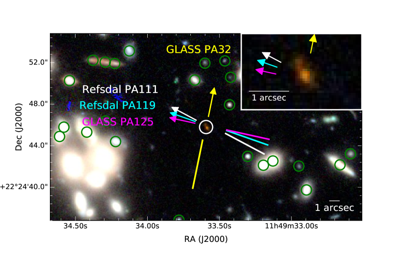
Figure 1.— Color composite image from the HST filters: F105W, F125W and F160W. MACS1149-JD is circled in white in the center of the image. The 4 grism dispersion directions are shown with the colored arrows. The labels on the arrows correspond to the PA_V3 header keyword, following the GLASS convention (Treu et al., 2015). The cluster core containing the brightest cluster galaxy (not shown) is approximately $1^{\prime}$ to the south of MACS1149-JD. The green circles show a subset of the objects whose spectra (of any order) have the potential to contaminate the spectrum of MACS1149-JD. We modeled these galaxies separately to obtain a global contamination model for MACS1149-JD. A zoomed in region centered on MACS1149-JD is shown in the upper right inset.

Table 1Photometry of MACS1149-JD

Filter	AB magnitude
F435W	$>27.84$
F606W	$>28.38$
F814W	$>28.53$
F105W	$>28.67$
F125W	$26.85\pm 0.07$
F140W	$26.00\pm 0.05$
F160W	$25.71\pm 0.03$
HAWK-I Ks	$>25.06$
IRAC CH1	$>25.52$
IRAC CH2	$24.79\pm 0.15$

Note. — ASTRODEEP (Di Criscienzo et al., 2017) photometry for MACS1149-JD used in this work. Limiting magnitudes are $3\sigma$. MACS1149-JD corresponds to source 2876 with $z_{\mathrm{phot}}=9.56$ in the ASTRODEEP catalog of MACS1149.

2.2. Slitless Grism Data

In addition to the significant investment of HST imaging, MACS1149 has been observed extensively with the HST near-infrared (NIR) grisms. Table 2 provides an overview of the spectroscopy we use in this work. MACS1149 was first observed with the HST G102 and G141 NIR grisms by the Grism Lens-Amplified Survey from Space (GLASS; Schmidt et al., 2014; Treu et al., 2015) in 2014. GLASS obtained 10 orbits in G102 and 4 orbits in G141, which together provide approximately uniform continuum sensitivity over the wavelength range $0.81-1.69\mu m$. The GLASS data were taken at two approximately orthogonal dispersion position angles to aid contamination subtraction and to provide two independent detections of real spectral features (Treu et al., 2015). While MACS1149-JD was not taken into consideration when the GLASS position angles were chosen, its first order spectra are contained in both with approximately equal exposure time in each position angle. We refer to the GLASS positions angles as P.A. $=32^{\circ}$ and P.A. $=125^{\circ}$ throughout.

The discovery of Supernova (SN) Refsdal (Kelly et al., 2015) in the MACS1149 prime field prompted a HST Director’s Discretionary Time program to obtain 30 additional orbits in G141 during 2014 December - 2015 January to determine the SN type (HST-GO-14041; Kelly et al., 2016) (hereafter the “Refsdal” data). The Refsdal data were taken at two position angles (P.A. $=111^{\circ}$, P.A. $=119^{\circ}$), which were optimized to reduce the contamination for extracting the spectrum of SN Refsdal. Both of these position angles contain the spectra of MACS1149-JD with approximately equal exposure time in each position angle. However, both position angles are separated by less than $25^{\circ}$ from the GLASS P.A. $=125^{\circ}$, the GLASS position angle in which MACS1149-JD is more contaminated. The dispersion directions corresponding to the two GLASS and two Refsdal position angles are indicated by the arrows in Figure 1.

The GLASS and Refsdal grism data were reduced together using the Grism redshift & line analysis software for space-based slitless spectroscopy (Grizli; Brammer et al. in preparation). We briefly outline the data reduction steps here. First, raw grism and direct exposures were obtained from the Mikulski Archive for Space Telescopes (MAST). In addition to grism exposures, both GLASS and Refsdal programs obtained direct images in HST to establish the wavelength zero points of the grism exposures. F105W and F140W were used to calibrate G102 and G141, respectively, due to similarity in wavelength coverage. The HFF F814W v1 mosaic was used for absolute astrometric calibration. Raw exposures containing bright satellite trails and high backgrounds due to the He Earth-glow were manually identified and discarded (Brammer et al., 2014). Variable sky backgrounds were accounted for as in Brammer et al. (2012). For each individual exposure we mask pixels where the MAST persistence model predicts persistent flux at a level greater than $0.6$ times the pixel flux uncertainty (Brammer, 2016).

Grism data from different visits were combined using Astrodrizzle (Gonzaga et al., 2012). The drizzled products consist of a two-dimensional cutout with two orthogonal axes: a spatial axis along the vertical and a calibrated wavelength axis along the horizontal. This process rectifies the trace of the spectrum along the horizontal axis, as opposed to, for example, the GLASS products and the spectra in O16, which were both reduced using the 3D-HST pipeline (Brammer et al., 2012) and have a noticeable spectral tilt. The grism products have, before drizzling, a spectral dispersion of $24.5$ Å/pix and $46.5$ Å/pix in G102 and G141, respectively. The G102 and G141 data provide a continuous spectrum of MACS1149-JD from $0.81-1.69\mu m$, although with varying sensitivity as a function of wavelength because the combined G141 spectrum is significantly deeper than G102. Nevertheless, the G102 data are included in this analysis as they are helpful for building the contamination model.

Table 2Spectroscopic data used in this work

Grism	P.A. (∘)	$N_{\mathrm{orbits}}$	$t_{\mathrm{exp}}(s)$	Program
G102	32	5	9826	GLASS
G102	125	5	10629	GLASS
G141	32	2	4412	GLASS
G141	125	2	4412	GLASS
G141	111	15	35788	Refsdal
G141	119	15	34988	Refsdal

Note. — The P.A. values are taken from the PA_V3 header keyword in the individual flt files, following the GLASS convention. Exposure times are rounded to the nearest second.

3. Contamination Modeling

We used Grizli to build a global contamination model by modeling each source for each visit and position angle. By working at an early stage in the reduction, the noise properties of each model unit are characterized more readily than after drizzling, which can produce correlated noise. Models from each visit can then be drizzled together for extraction of spectral features from the full-depth data.

The global contamination model requires three components: a reference image for image/grism alignment, a segmentation image and a Source Extractor (SExtractor; Bertin & Arnouts, 1996) photometric catalog associated with the segmentation image. For the reference image, we used a full depth HST WFC3/IR F160W mosaic created by co-adding all of the available F160W for MACS1149 data on MAST, as of November 2016. We used the segmentation map and associated source catalog provided by GLASS. The segmentation map was created from the stack of the CLASH NIR bands using the CLASH SExtractor parameters, and the GLASS team used this segmentation map to perform contamination subtraction on their own data (Schmidt et al., 2014; Treu et al., 2015). We did not notice a significant difference in the resulting model when using a segmentation image created from the full-depth HFF images, as expected because the contamination is dominated by bright sources.

First, a simple flat (in $F_{\lambda}$) spectrum model was assigned to every object in the segmentation map satisfying $H_{160}<25$, where the normalization of the model was determined by the flux in the F160W reference image. Then, a second order polynomial was fit to each object in the flat model satisfying $16<H_{160}<24$. This last step is iterated until differences in the global contamination model become negligible, which in our case occurred after three total iterations.

In an attempt to more carefully model the contamination affecting the trace of MACS1149-JD, we performed another tier of modeling on top of what is described above. We searched the segmentation map for all sources that could possibly contaminate the first order spectrum of MACS1149-JD in each of the four position angles. This amounted to selecting all objects at least as bright ($H_{160}<25.6$) as MACS1149-JD that fall within $\pm 1\farcs 8$ of the expected trace of MACS1149-JD in all four position angles. The size of the search beam was chosen so that off-center extended objects would also be flagged. 164 objects satisfied these criteria. We then visually inspected each of these objects in the HFF v1 images as well as the segmentation image. We found that 14 of these objects were likely spurious, either because they lacked a counter-part in the deep HST images or because they were part of a diffraction spike.

For the 150 remaining objects (some shown in Figure 1), which we deemed were primary contaminants of MACS1149-JD, we refined their models further by performing spectral energy distribution (SED) fitting of the grism data. Grizli performs SED fitting by comparing two-dimensional grism models from, in our case, a minimal set of galaxy templates to two-dimensional cutouts of each object’s first order spectrum. Briefly, we considered four templates:

• A very young, low metallicity Lyman-break galaxy (LBG) based on Q2343-BX418 (Erb et al., 2010)

• An intermediate age SED with a moderate 4000 Å break (D4000)

• An old simple stellar population from Conroy & van Dokkum (2012)

• A post-starburst template with prominent Balmer break and strong D4000

In addition to the templates, a set of emission lines with fixed line ratios are included in the fit. The emission lines are useful for breaking redshift degeneracies. The redshift fitting was first run over a coarse grid ($\Delta z=0.01$) over the interval $0.5<z<2.3$. This range was chosen based on the reliability of detecting strong emission lines in G102 and G141 at these redshifts. The templates are flexible enough to provide an improved description of the continua over a simple polynomial model even if the redshifts are incorrect. A second, finer grid ($\Delta z=0.002$) was run around the best-fit peaks (determined by the $\chi^{2}$) in the first grid. The best-fit redshift found during the second, finer redshift grid was assigned to the galaxy.

The top four panels of Figure 2 show the drizzled contamination models from each position angle at the location of the first order spectrum of MACS1149-JD. The bottom panel shows the stack of all four position angles. Although the two Refsdal position angles are 15 orbits each in G141, compared to the 2 orbits each for the two GLASS position angles, the Refsdal P.A. $=111^{\circ}$ is severely contaminated along the trace of MACS1149-JD. Furthermore, the contamination in this P.A. is dominated by the second order spectrum of a bright galaxy (not shown in Figure 1). Grizli fits to the first order spectra, while the second order spectra of contaminants are determined from a calibration between first and higher order spectra, which is in general less accurate than direct modeling. The other three position angles are much cleaner of contamination. As a result, we discard the Refsdal P.A. $=111^{\circ}$ data in our analysis.

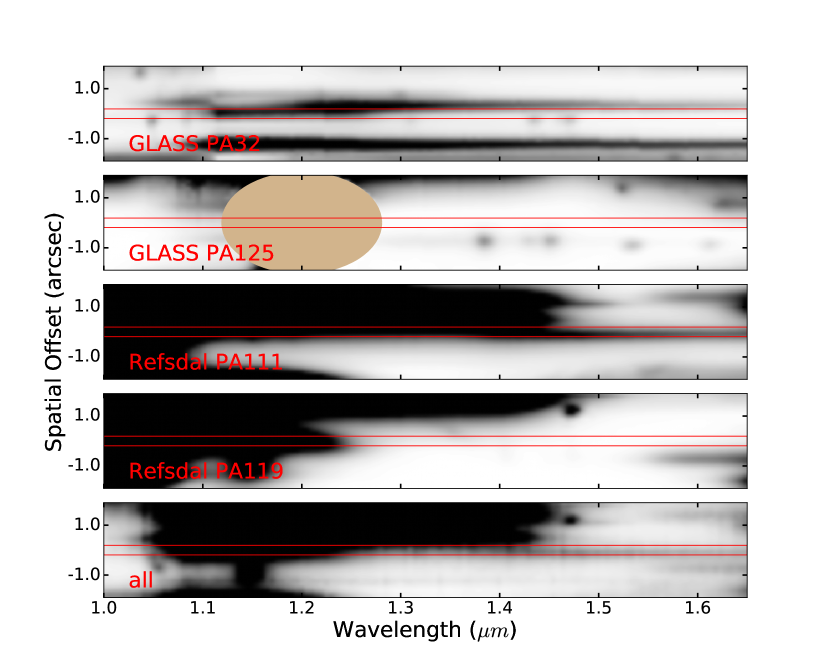
Figure 2.— Contamination models for each of the 4 individual orients as well as the stack (bottom) extracted near the trace of MACS1149-JD (red horizontal lines). P.A. $=111^{\circ}$ is severely contaminated over the entire trace. The contamination is dominated by the second order trace of a bright object, making the contamination in this orient especially difficult to model. Black represents positive signal. The tan ellipse in GLASS P.A. $=125^{\circ}$ masks out a large detector artifact.

4. Continuum Extraction

We show the two-dimensional contamination-subtracted spectrum of MACS1149-JD combined from the two GLASS position angles and the single Refsdal P.A. $=119^{\circ}$ in the top panel of Figure 3. The final spectrum is an inverse variance weighted stack of the 3 position angles, totaling 19 orbits of G141. The contamination was not included in the variance array when stacking (see Section 5.3). However, we down-weighted an especially contaminated off-trace portion of the GLASS P.A. $=32^{\circ}$ spectrum for display purposes only (see the Appendix).

The one-dimensional spectrum shown in the bottom panel of Figure 3 was obtained by summing within a 3 pixel ($0\farcs 38$) aperture along the spatial (vertical) axis of the two-dimensional spectrum. A positive signal is detected in the one-dimensional spectrum at $\lambda\gtrsim 1.25~{}\mu m$. The median signal-to-noise ratio ($S/N$) per $50$ Å bin is $1.1$ over the continuous interval $1.25<\lambda<1.65~{}\mu m$, whereas it is $S/N=0.2$ at $\lambda<1.25~{}\mu m$. The integrated $S/N$ over the interval $12500<\lambda<16500$, is $(S/N)_{\mathrm{total}}=11.1$. We also performed a Horne (1986) extraction, but the increase in $S/N$ of the detection was negligible in comparison to the simple sum. In Figure 3 we also show the one-dimensional contamination spectrum and rms noise spectrum extracted using the same size spatial aperture.

In the process of extracting the one-dimensional spectrum, we also subtracted a local background, which we computed by taking the median in each column of the data array after masking out contaminated pixels. We used a variety of thresholds when masking to assess the change in the background. We varied the threshold based on the fraction of the mean contamination level in the entire two-dimensional contamination array, ranging from 0.05 to 1 times the mean contamination, in steps of 0.05. We then applied these masks to the data array and calculated the median in each column. The median and standard deviation of the backgrounds calculated at each threshold level were used as the background and the error on the background in our spectral extraction. Before background subtraction, the mean value of the pixels outside of the trace of MACS1149-JD was $-1.51^{+1.08}_{-0.37}\,\times 10^{-19}~{}\mathrm{erg\,s^{-1}\,cm^{-2}\,pix^{-1}}$, whereas after background subtraction we obtained $-0.01^{+0.29}_{-0.19}\,\times 10^{-19}~{}\mathrm{erg\,s^{-1}\,cm^{-2}\,pix^{-1}}$. Therefore, we successfully subtracted the negative background, although some slight positive off-trace residuals remain, which we discuss in the Appendix. We note that the error bars on the one-dimensional spectrum shown in Figure 3 incorporate the rms noise and the uncertainty on the background.

We show several tests of the validity of the continuum detection in the Appendix. Most importantly, when the GLASS and Refsdal data are separated, the bulk of the positive signal observed in Figure 3 arises from the deeper Refsdal data (Figure A1). While there are contamination residuals away from the trace of MACS1149-JD (Figure A3), the lack on contamination along the trace of MACS1149-JD indicates that the positive signal is unlikely to arise from a contamination residual.

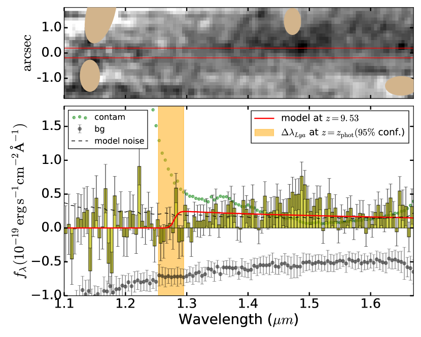
Figure 3.— Top: 2D contamination-subtracted grism spectrum of MACS1149-JD from the 3 reliable position angles. Black represents positive signal. The tan ellipses mask out 0th order contamination residuals. The 2D spectrum was smoothed with a 2D Gaussian kernel with $\mathrm{FWHM}=2$ pixels in both dimensions to bring out the continuum feature. Bottom: 1D spectrum (yellow histogram) extracted from the spatial aperture denoted by the red lines in the top panel. The red line shows the predicted signal from a Lyman-break galaxy model at the most probable redshift derived from the grism data ($z=9.53$, see Section 5.3), normalized to the HST F160W magnitude. The black dashed line shows the predicted noise level in the absence of contamination. The shaded yellow region indicates the wavelength range where Ly$\alpha$ would be expected from the 95% confidence interval on the photometric redshift. While we do not detect Ly$\alpha$ emission, a positive signal is detected above the noise level at $>1.25~{}\mu m$, which is likely the continuum from MACS1149-JD. Both the 2D and 1D spectra are drizzled to $50$ Å $/$ pixel.

5. Redshift estimation

5.1. Photometric Redshift

The photometric redshift was measured using the methodology described by Huang et al. (2016). In brief, we used the code EAZY (Brammer et al., 2008) along with the stellar population templates from Bruzual & Charlot (2003, hereafter BC03), a Chabrier (2003) initial mass function between $0.1$ and $100M_{\odot}$, a Calzetti et al. (2000) dust attenuation law, and an exponentially declining star formation history (SFH) with a fixed metallicity of 0.2 $Z_{\odot}$. Nebular emission lines were added to the galaxy templates as in Huang et al. (2016).

The photometric data used to constrain the redshift are from the ASTRODEEP catalogs and are summarized in Table 1. The data are extremely deep and span the interval from $\sim 0.4-5\mu m$. Figure 4 shows the best-fit spectral energy distribution (SED) template and the photometric detections and $3\sigma$ upper limits for MACS1149-JD. The photometric redshift distribution (hereafter $P(z)$) is shown in the inset in Fig 4 below the SED. The best-fit photometric redshift is $z=$ $9.51^{+0.06}_{-0.12}$ (68% confidence). This is in agreement with recent estimates of the photometric redshift, for example $z=9.44\pm 0.12$ obtained by Zheng et al. (2017), who used the same imaging data except for the MOSFIRE Ks-band, which does not provide strong additional constraints on the SED. The Spitzer/IRAC CH1 and CH2 data are much more important. For example, if we exclude CH1 and CH2 from our photometry, the 68% confidence interval on the photo-$z$ is $[9.22,9.68]$, a factor of $2.5$ broader than when including CH1 and CH2.

Interestingly, Zheng et al. (2017) report a $S/N=5.9$ detection in IRAC CH1, i.e. a magnitude of $25.64\pm 0.17$. In the ASTRODEEP catalog (Table 1), MACS1149-JD is not detected in CH1 above the $3\sigma$ level. We also performed independent photometry on the full depth HFF HST and IRAC data using the method described by (Huang et al., 2016), similarly not detecting MACS1149-JD in CH1 above $3\sigma$. Whether CH1 is considered a detection or not, this does not seem to significantly affect the inferred photometric redshift; the photo-$z$’s obtained by Zheng et al. (2017) and ASTRODEEP are in statistical agreement, as we saw above. Huang et al. (2016) obtained a slightly lower photometric redshift, $z=9.3\pm 0.1$ for MACS1149-JD, but using shallower IRAC data than in Zheng et al. (2017) and in this work.

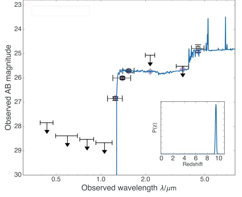
Figure 4.— Best-fit spectral energy distribution (SED) for MACS1149-JD from ASTRODEEP photometry. The purple diamonds represent the magnitudes of the SED integrated over each filter bandpass. The photometric data are summarized in Table 1. Downward facing arrows represent $3\sigma$ upper limits.

5.2. Search for Lyman-alpha emission

We first searched the grism data for emission lines within the wavelength range inferred from the photometric redshift, $9.31<z<9.65$ (95% confidence). This interval corresponds to the wavelength range $1.254<\lambda<1.295~{}\mu m$, which is denoted by the yellow shaded region in the bottom panel of Figure 3. The spectrum is consistent with the noise in this interval, so Ly$\alpha$ is not significantly detected above our flux limit.

To estimate the Ly$\alpha$ flux limit, we used the same method and the same aperture ($0\farcs 6\times 100$ Å) as Schmidt et al. (2016), who calculated flux limits for 47 $z\gtrsim 7$ LBG candidates in 6 of the GLASS clusters, MACS1149 not included, throughout G102 and G141. Schmidt et al. (2016) found median $1\sigma$ Ly$\alpha$ flux limits of $4-6\times 10^{-18}~{}\mathrm{erg\,s^{-1}cm^{-2}}$ (95% confidence) per 2-orbit G141 position angle in the photo-$z$ wavelength range, $1.254<\lambda<1.295~{}\mu m$, before taking into account magnification. As a cross-check, we measured the $1\sigma$ flux limit in this wavelength range using the GLASS P.A. $=32^{\circ}$ orient alone, finding $5.3\times 10^{-18}~{}\mathrm{erg\,s^{-1}cm^{-2}}$, in agreement with the range found by Schmidt et al. (2016) for observations of the same depth.

With the addition of the Refsdal data, we achieve a more sensitive Ly$\alpha$ flux limit of $1.8\times 10^{-18}~{}\mathrm{erg\,s^{-1}cm^{-2}}$ ($1\sigma$), before taking into account magnification. The limit was obtained using the GLASS P.A. $=32^{\circ}$ and Refsdal P.A. $=119^{\circ}$ data, but not the other two position angles. The Refsdal P.A. $=111^{\circ}$ data were not included for the reasons described in Section 4 and in the Appendix, and the GLASS P.A. $=125^{\circ}$ data were not included because of a detector artifact present in the wavelength range where Ly$\alpha$ would be expected from the photometric redshift (Figure 2). The Ly$\alpha$ flux limit can be converted into a limit on the Ly$\alpha$ equivalent width (EW) since the continuum redward of the expected position of the Ly$\alpha$ line and the Ly$\alpha$ break is detected in HST imaging. Within the wavelength range $1.254<\lambda<1.295~{}\mu m$, the only HST filter sampling the rest-frame UV in which the Ly$\alpha$ emission line and the Ly$\alpha$ break do not fall is F160W. Adopting the F160W magnitude as the baseline continuum level, we estimate a $3\sigma$ rest-frame Ly$\alpha$ EW limit of $21$ Å. For comparison, the same limit is $63$ Å in the GLASS P.A. $=32^{\circ}$ data alone. Bian et al. (2015) obtained ground-based spectroscopy with LBT/LUCI (Ageorges et al., 2010; Hill et al., 2012) of MACS1149-JD over the wavelength interval $1.17-1.30~{}\mu$m, and similarly did not detect Ly$\alpha$ emission. For comparison, they obtained $3\sigma$ rest-frame Ly$\alpha$ EW limits of $\sim 30$ Å over the interval $1.17<\lambda<1.26~{}\mu$m and $\sim 50$ Å over $1.26<\lambda<1.30~{}\mu$m.

We calculated the probability of observing this EW limit in the context of a likely highly neutral universe (Planck Collaboration et al., 2016; Greig & Mesinger, 2017) using the method from Mason et al. (2017). In brief, we take reionization simulations of the IGM by Mesinger et al. (2016) for different values of the neutral hydrogen fraction, $f_{\mathrm{HI}}$, and populate halos with LBG properties calibrated using the observed Ly$\alpha$ EW distribution at $z=6$ to obtain EW distributions as a function of $f_{\mathrm{HI}}$ and $M_{UV}$. We consider two scenarios: 1) a completely ionized universe, i.e. $f_{\mathrm{HI}}=0$ and 2) a more realistic universe with $f_{\mathrm{HI}}=0.75$. We find $p(\mathrm{EW}<7$ Å$)=0.32$ in case 1) and $p(\mathrm{EW}<7$ Å$)=0.52$ in case 2). Hence the non-detection is not surprising in either case, but especially so in the mostly neutral universe. We note that the simulations are for $z=7$. At $z=9.5$, the Ly$\alpha$ line from this galaxy would be further damped since the decreased cosmic volume would put MACS1149-JD in closer proximity to neutral patches. Thus at $z=9.5$ our observation is even more likely than the numbers quoted above for $z=7$.

5.3. MCMC analysis

Because the grism data are sensitive enough to detect the continuum of MACS1149-JD, the search for the Ly$\alpha$ emission line in the remaining portion of the grism data is more complicated; a detection of Ly$\alpha$ emission is degenerate with a marginal detection of the continuum. To quantify this degeneracy, we performed a Markov chain Monte Carlo (MCMC) analysis with redshift ($z_{g}$), rest-frame Ly$\alpha$ EW ($\mathrm{EW}_{Lya}$), and F160W magnitude ($m160$) as parameters.

We generated one-dimensional LBG models with fixed rest-frame UV slope of $\beta=-2$ (c.f. Bouwens et al., 2014) at $z=0$ and set all flux blue-ward of the rest-frame Ly$\alpha$ wavelength to zero. We then redshifted these templates to $z_{g}$ and added a Ly$\alpha$ emission line with a rest-frame EW of $\mathrm{EW}_{Lya}$. The intrinsic FWHM of the line we used is $150~{}\mathrm{km}~{}s^{-1}$, although due to the low resolution of the grism the FWHM does not significantly influence the results. We normalized the models so that their integrated F160W magnitude equaled $m160$. The one dimensional models were then convolved with the object’s 2D morphology for each individual exposure (with its given P.A.) and the exposure models were drizzled exactly as with the data spectrum shown in Figure 3. While the object is clearly resolved, as is visually apparent in Figure 1, the compact central clump dominates the surface brightness. Because the surface brightness distribution of the object is used when drizzling the 1D models to 2D, the extended portion of the galaxy does not significantly contribute to the 2D drizzled model. The red line shown in Figure 3 is the 1D extraction from the 2D drizzled model using the same aperture as the one used to extract the data.

We used the MCMC sampler from the Python package emcee (Foreman-Mackey et al., 2013) to obtain the posterior probability distributions on the three parameters. We used a flat prior on the redshift over $z\in[8.0,11.5]$, the interval to which the G141 grism data are sensitive for the LBG model. We used a Gaussian prior on $m160$, with center and standard deviation given by the isophotal magnitude and uncertainty in F160W. The isophotal magnitude is the correct normalization magnitude because we use the segmentation image to define the extent of the two-dimensional models. The ASTRODEEP catalog does not provide isophotal magnitudes, so we measured these independently using SExtractor in dual-image mode with the same parameter settings employed in Section 3, finding $\mathrm{MAG\_ISO_{F160W}}=25.63\pm 0.06$. This is brighter than the total magnitude in the ASTRODEEP catalog reported in Table 1, which is due to a different estimation of the local background. ASTRODEEP performed an ICL subtraction on the F160W image, whereas we did not. While MACS1149-JD is distant from the cluster center where the ICL contribution is the highest, there is still a small contribution near MACS1149-JD, explaining why our magnitude is brighter than the ASTRODEEP magnitude. Because the isophototal magnitude is only used to normalize the MCMC models and is never compared to the ASTRODEEP photometry, this discrepancy does not affect our results. Finally, we adopted a half Gaussian prior on $\mathrm{EW}_{Lya}$, centered on zero with standard deviation of $15$ Å, accepting only positive values because we are not sensitive to Ly$\alpha$ absorption. We used the following log-likelihood function in the MCMC sampler:

$$ln(\mathcal{L})\sim-\chi^{2}/2=-\frac{1}{2}\sum_{i}\frac{(f_{i}-m_{i})^{2}}{\sigma_{i}^{2}},$$

where $f_{i}$, $m_{i}$, and $\sigma_{i}$ are the pixel values in the flux, model and uncertainty arrays, respectively. The uncertainty consists of the detector noise and the background noise (see Section 4) added in quadrature. With this prescription, we found a reduced $\chi^{2}$ close to 1 for the best-fit parameters. We also experimented including contamination into the uncertainty array, but found that we over-fit the data by doing so. Therefore, we did not include contamination uncertainty in the uncertainty in the log-likelihood.

The resulting corner plot for the 3 MCMC parameters is shown in Figure 5. The top left panel of the bottom sub-figure shows the marginalized likelihood for the redshift derived from the grism alone. This is also plotted on the top sub-figure for comparison with the photo-$z$. The best-fit redshift derived from the grism alone is $z_{\mathrm{grism}}=9.53^{+0.39}_{-0.60}$ (68% confidence), consistent with the photometric value of $z_{\mathrm{phot}}=9.51^{+0.06}_{-0.12}$. The grism redshift is much more uncertain than the photometric redshift, unsurprising given the level at which the continuum is detected in the grism. The combined likelihood is shown in red, with a best fit value of $z_{\mathrm{comb}}=9.49^{+0.06}_{-0.08}$ (68% confidence).

The other two MCMC parameters of the LBG model are $m160$ and $\mathrm{EW}_{Lya}$. The posterior for $m160$ is very similar to the prior, indicating that the grism spectra are not especially sensitive to this parameter. The fact that there is agreement with the photometric value serves as a sanity check. We derive an upper limit of $\mathrm{EW}_{Lya}<6$ Å ($1\sigma$) over the interval $8<z<11.5$, similar to what we found in the previous section using a different method ($\mathrm{EW}_{Lya}<7$ Å). This corresponds to a $1\sigma$ Ly$\alpha$ flux limit of $1.5\times 10^{-18}~{}\mathrm{erg\,s^{-1}cm^{-2}}$.

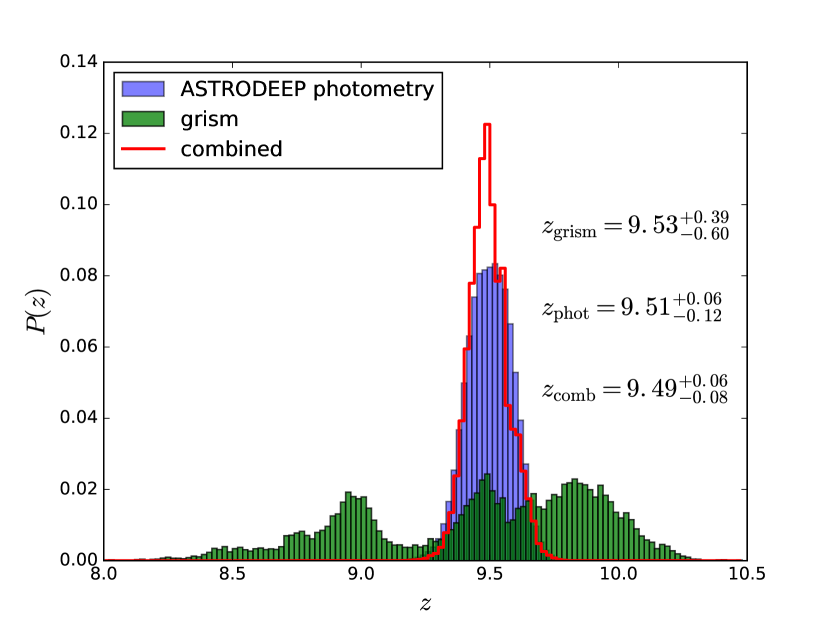
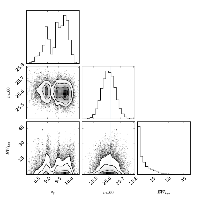
Figure 5.— Top: Normalized redshift distributions inferred from photometry alone (blue histogram), from the grism alone (green histogram), and from multiplying the two distributions (red line). Bottom: Corner plot from MCMC fitting the grism data (excluding the contaminated Refsdal P.A. $=111^{\circ}$) to Lyman break galaxies models, where the three model parameters are the redshift $z_{g}$, the F160W normalization magnitude ($m160$), and the Ly$\alpha$ equivalent width ($\mathrm{EW}_{Lya}$). The blue line indicates the value of MAG_ISO measured in F160W, in good agreement with the F160W magnitude inferred from the grism data.

6. Gravitational Lens Model

In order to constrain many of the intrinsic properties of MACS1149-JD, a lens model of the galaxy cluster, MACS1149, is required. Since the original gravitational lens models by Smith et al. (2009); Zitrin & Broadhurst (2009), MACS1149 has been modeled extensively. As part of the version 1 (v1) HFF call for lensing models in 2013, before the HFF imaging took place, we created a strong and weak gravitational lens model of MACS1149 using the Strong and Weak Lensing United (SWUnited; Bradač et al., 2005, 2009) code. We have since modeled the cluster using constraints from the full-depth HFF imaging and HST grism spectroscopy from GLASS and the SN Refsdal follow-up program (Treu et al., 2016). The magnification from the newer model presented by Finney et al. (in preparation) is $\mu_{\mathrm{best}}=$ $18.6^{+4.3}_{-2.6}$ (68% confidence). This model will be referred to as the Bradac v4 model. Our magnification factor is in agreement with the median magnification from the six other publicly available post-HFF lens models: $\mu=$ $9.0^{+41.0}_{-5.1}$.

7. Discussion

7.1. Physical properties of MACS1149-JD

The recovered physical properties of MACS1149-JD are listed in Table 3. These were obtained by using the combined grism$+$photometric redshift distribution as a prior in the SED fitting procedure outline in Section 5.1. As inferred by previous authors (Zheng et al., 2012; Huang et al., 2016; Zheng et al., 2017), the galaxy is intrinsically faint and low mass due to its large, albeit uncertain, magnification. Using the Bradac v4 magnification factor obtained by Finney et al. (in preparation), $\mu_{\mathrm{best}}=$ $18.6^{+4.3}_{-2.6}$, and the observed F160W magnitude, we calculated the rest-frame absolute UV magnitude to be $M_{\mathrm{UV}}-2.5\,\mathrm{log}_{10}(\mu/\mu_{\mathrm{best}})=$ $-18.5\pm 0.1$ mag, or $<0.15L_{\star}(1\sigma)$, adopting $L_{\star}$. The factor $\mu/\mu_{\mathrm{best}}$ is introduced to parameterize our uncertainty on the magnification.

The most striking property of MACS1149-JD is its relatively large age of $340^{+29}_{-35}$ $\mathrm{Myr}$. The inferred age is primarily driven by the red color in Spitzer/IRAC: $\mathrm{CH1}-\mathrm{CH2}>0.73$ $(3\sigma)$, which was interpreted as a Balmer/4000 Å break by the SED fitting code (Figure 4). We note that the inferred age in general depends on the assumed SFH. We used an exponentially declining SFH to derive the age of $340^{+29}_{-35}$ $\mathrm{Myr}$. Adopting an exponentially rising SFH instead, we infer an age consistent within the statistical uncertainties of the age derived using exponentially declining SFH. The age of the galaxy, given the peak combined redshift, would indicate an onset of star-formation of only $\sim 200$ Myr after the Big Bang. By comparison, O16 spectroscopically confirmed a galaxy at higher redshift ($z=11.09$), yet the age of $<110$ Myr ($1\sigma$) implies an onset of star formation at $\gtrsim 300$ Myr after the Big Bang, later than what is inferred for MACS1149-JD.

From the theoretical side, the inferred age of $340^{+29}_{-35}$ $\mathrm{Myr}$ at $z=9.5$ is highly improbable. Using the luminosity function model from Trenti et al. (2015), we computed the halo assembly time for a $log_{10}(M_{h}/M_{\odot})=10.5$ halo at $z=9.5$, finding a median time of $65~{}\mathrm{Myr}$, and an upper limit of $<155~{}\mathrm{Myr}$ (99% confidence). The fact that the inferred age of MACS1149-JD is much larger than the upper limit on the assembly time is therefore surprising. If the age estimate is correct, it would require star formation well before the halo assembly time.

7.2. Interpretation of rest-frame optical observations

The age estimate of $340^{+29}_{-35}$ $\mathrm{Myr}$ is strongly dependent on the photometric redshift estimate, which is driven by the interpretation of the IRAC color as a continuum break. Recent observations of $z\sim 7$ LBGs have revealed that this population on average has strong rest-frame optical emission lines that are capable of boosting IRAC CH1 and/or CH2 fluxes by up to $\sim 1$ mag (e.g. Schaerer & de Barros, 2009; Shim et al., 2011; Labbé et al., 2013; de Barros et al., 2014; Smit et al., 2014; Castellano et al., 2017). For example, Smit et al. (2014) showed that $z\sim 7$ LBGs have average [O iii]$+H\beta$ equivalent widths of $>640$ Å. We investigated whether MACS1149-JD could possess similarly large emission line strengths that could explain the IRAC color of $\mathrm{CH1}-\mathrm{CH2}>0.73$ $(3\sigma)$. This would clearly change the physical interpretation of the galaxy, particularly the age.

First, we estimated the photo-$z$ without the IRAC CH1 and CH2 fluxes, eliminating the rest-frame optical constraints on the SED, which could bias the redshift inference. The 95% confidence interval of the resulting redshift likelihood function was $[8.93-9.77]$, about a factor of 2 broader than when including the IRAC data. This is consistent with the photometric redshift obtained by Kawamata et al. (2016), $z=9.2\pm 1.0$, who used the full depth HFF data but no IRAC or Ks-band data. We then multiplied this distribution with the grism likelihood distribution obtained in Section 5.3. The 95% confidence interval of the combined likelihood function was $[8.95-9.77]$, very similar to the range from the photometry alone. Over this interval, [O ii] always falls in CH1, $H\beta$ falls in CH2 for $z\lesssim 9.4$, and [O iii] falls in CH2 for $z\lesssim 9.2$.

We explored adding [O ii]$\lambda 3727$, [O iii]$\lambda\lambda 4959,5007$, H$\beta$, the remaining Balmer lines, and common metal lines (see Table 1 of Anders & Fritze-v. Alvensleben, 2003) in emission onto a redshifted $10~{}\mathrm{Myr}$ template spectrum (with no emission lines originally added) generated from the BC03 models assuming $Z=0.2Z_{\odot}$, $Z=0.02Z_{\odot}$, and $Z=Z_{\odot}$ to see if we could reproduce the IRAC color. We added in the $H\beta$ emission line, varying the rest-frame EW from $0-10000$ Å, and we calculated the rest-frame EWs of the other lines using the fixed flux ratios determined by Anders & Fritze-v. Alvensleben (2003), given the template metallicity. The continuum flux densities in CH1 and CH2 used to convert between EW and line flux were determined by integrating the templates over the respective bandpasses. We explored the redshift range given by the 95% confidence interval on the combined redshift derived above $z\in[8.95-9.77]$ in steps of $\Delta z=0.05$.

At $z>9.3$, the IRAC color cannot be recovered with $\mathrm{EW}_{H\beta}<10000$ Å (equivalently: $\mathrm{EW}_{[OIII]+H\beta}\lesssim 50000$ Å) for any of the input metallicities, as expected because the strongest emission line that we included, the [O iii] pair, falls redward of CH2. Therefore, strong rest-frame optical lines are unlikely to cause the red IRAC color if the redshift is $z>9.3$. At $9.05\leq z\leq 9.3$, we find that $\mathrm{EW}_{H\beta}\sim 800-1100$ Å ($\mathrm{EW}_{[OIII]+H\beta}\sim 4300-5800$ Å) are required to reproduce the IRAC color, larger than the equivalent widths observed by Smit et al. (2014). We note that these rest-frame equivalent widths are for the $Z=0.02Z_{\odot}$ case, with higher metallicities requiring much larger equivalent widths to reproduce the IRAC color.

However, in the range $8.95\leq z<9.05$, we are able to reproduce the IRAC color with precedented values of $\mathrm{EW}_{H\beta}$.The equivalent widths required to do so are $\mathrm{EW}_{H\beta}\sim 425-550$ Å ($\mathrm{EW}_{[OIII]+H\beta}\sim 2200-2900$ Å) for $Z=0.02Z_{\odot}$ or $\mathrm{EW}_{H\beta}\sim 350-375$ Å ($\mathrm{EW}_{[OIII]+H\beta}\sim 2500-2800$ Å) for $Z=0.2Z_{\odot}$. These equivalent widths are consistent with the sample from Smit et al. (2014), where they measured $\mathrm{EW}_{[OIII]+H\beta}$ from HST-selected $z\sim 7$ galaxies in cluster fields. They are also consistent with $\mathrm{EW}_{[OIII]+H\beta}$ measured for the Green Peas (Henry et al., 2015) and from metal-poor local dwarf galaxies specifically selected to show He ii (Senchyna et al., 2017). We note, however, that there is only a 5% chance that the redshift is $z<9.05$, based on the joint grism$+$photometric redshift distribution once IRAC constraints are dropped. While one of the peaks of the grism redshift distribution occurs around $z\sim 9$, the HST photometry (even after neglecting the IRAC constraints) provide the tightest constraints against lower redshifts. This exercise demonstrates that the HST photometry, Spitzer/IRAC photometry and grism spectra are all consistent with a $10~{}\mathrm{Myr}$, sub-solar metallicity galaxy with strong rest-frame optical nebular emission lines, but only in the low-redshift tail of the redshift distribution.

The reason our SED-fitting process was unable to fit nebular emission lines with such large equivalent widths is due to the manner in which they were added to the BC03 templates. We used the relation from Leitherer & Heckman (1995) to scale the Lyman continuum flux predicted by the BC03 templates to the $H\alpha$ flux. We then used the flux ratios from Anders & Fritze-v. Alvensleben (2003) given the template metallicity to get the fluxes of the other nebular emission lines. For a 10 Myr old, $Z=0.02Z_{\odot}$ template, the maximum rest-frame $\mathrm{EW}_{H\beta}\sim 100$ Å. This is $\sim 250$ Å lower than the minimum rest-frame $\mathrm{EW}_{H\beta}$ necessary to produce the IRAC color. At higher metallicities, the emission line strengths predicted from the models are even lower. While we used $Z=0.2Z_{\odot}$ templates when performing SED fitting, a lower metallicity template similarly would not have been able to fit the IRAC photometry with strong nebular emission lines. Because larger EWs are observed in practice at $z\sim 7$ (e.g. Smit et al., 2014), the prescription we use for adding nebular emission may be inappropriate here. Rest-frame optical spectroscopy with the James Webb Space Telescope of $z\gtrsim 7$ galaxies will provide direct measurements of the nebular line strengths. These measurements will be able to break the degeneracy between the Balmer/$4000$ Å break and strong rest-frame optical emission lines for MACS1149-JD.

Table 3Properties of MACS1149-JD

$\mathrm{R.A.}$	(∘)	177.38997
$\mathrm{Dec.}$	(∘)	22.412722
$z_{\mathrm{grism+photometry}}$		$9.49^{+0.06}_{-0.08}$
$\mu_{\mathrm{best}}(z=$$9.49^{+0.06}_{-0.08}$)		$18.6^{+4.3}_{-2.6}$
$M_{\mathrm{UV}}-2.5\,\mathrm{log}_{10}(\mu/\mu_{\mathrm{best}})$	(mag)	$-18.5\pm 0.1$
$M_{\star}\times\mu/\mu_{\mathrm{best}}$	($10^{8}M_{\odot}$)	$5.8^{+0.9}_{-0.9}$
$L_{\mathrm{UV}}\times\mu/\mu_{\mathrm{best}}$	($L_{\star}$)	$0.14\pm 0.01$
$SFR\times\mu/\mu_{\mathrm{best}}$	($M_{\odot}/\mathrm{yr}$)	$0.7^{+0.6}_{-0.2}$
Age	($\mathrm{Myr}$)	$340^{+29}_{-35}$
$E(B-V)$	mag	$<0.01$
$\mathrm{EW}_{Lya}$ ($3\sigma$)	Å	$<21$

Note. — The absolute rest-frame UV magnitude is determined using the F160W magnitude to calculate the underlying continuum flux density. The magnification used to correct the absolute UV magnitude, stellar mass and star formation rate are from the Bradac v4 model.

8. Summary

We presented deep grism-spectroscopic observations of MACS1149-JD, one of the highest redshift galaxies known. We tentatively detected the rest-frame UV continuum in the combined HST G141 data, although contamination residuals near the trace of MACS1149-JD make this detection somewhat uncertain. We used an MCMC fitter to constrain a simple LBG model with three parameters, ($z$, F160W mag, and rest-frame Ly$\alpha$ EW). We found that the redshift and F160W magnitude inferred by the grism data are consistent with our photometric measurements, as well as those from the literature using the same quality photometry. The grism data provide the most constraining upper limit on Ly$\alpha$ emission for this galaxy to date, ruling out Ly$\alpha$ in emission above an equivalent width of $21$ Å ($3\sigma$).

The grism data support the interpretation of the red Spitzer/IRAC $\mathrm{CH1}-\mathrm{CH2}$ color as a Balmer/4000 Å break, as well as the strong rest-frame optical emission lines boosting the CH2 flux. The strong emission line scenario is less preferred by the HST photometry but cannot be completely ruled out. The preferred interpretation implies that the galaxy fosters a stellar population that is at least $\sim 300~{}\mathrm{Myr}$ old already at $z=$$9.49^{+0.06}_{-0.08}$, the combined grism$+$photometric redshift. If this interpretation of the IRAC color is correct, then this implies that MACS1149-JD formed around $200~{}\mathrm{Myr}$ after the Big Bang, making it one of the earliest sites for star-formation known to date.

Testing the validity of the continuum detection in G141

In this appendix we show several tests for determining the validity of the continuum detection in the presence of contamination.

If the continuum detection in the stack of all three orients shown in Figure 3 is real, it should come primarily from the deeper Refsdal P.A. $=119^{\circ}$ data. We show the spectra from combining the two GLASS orients as well as the individual Refsdal P.A. $=119^{\circ}$ data in Figure A1. The stacked GLASS spectra are consistent with the noise, whereas the Refsdal P.A. $=119^{\circ}$ data are consistently above the noise. Thus the majority of the signal in the stack comes from the Refsdal P.A. $=119^{\circ}$ data. We verified that the signal does not arise from a single exposure or visit within the Refsdal P.A. $=119^{\circ}$ data. When divided in half, the Refsdal P.A. $=119^{\circ}$ data show a similar signal in both data sub-sets.

The spectra in Figure A1 extend out to $1.7~{}\mu m$, the edge of the G141 grism. At $\lambda\geq 1.65~{}\mu m$, the throughput of G141 drops quickly, which should in principle be reflected by the spectrum of a real object. In our case, contamination rises in both the GLASS and Refsdal P.A. $=119^{\circ}$ at these wavelengths. As a result, we cannot reliably use this test to determine the validity of our spectrum.

The continuum magnitude derived in the grism is somewhat brighter than the expectation from the photometry. For example, if we integrate the grism flux density from the 3 good position angles within a $0\farcs 38$ spatial aperture over the F160W bandpass, which is entirely contained in G141, we get a magnitude of F160W (grism) $=25.5\pm 0.1$, compared to a photometric magnitude of F160W (imaging) $=26.1\pm 0.1$ using a spatial aperture of the same size. We note that this photometric magnitude is fainter than the magnitude reported in Table 1 because of the smaller aperture used in this test. The photometric magnitude is measured by creating a flat spectrum that is normalized to F160W $=\mathrm{MAG\_ISO}$, and then convolving this spectrum with the segmentation image of MACS1149-JD, drizzling it to a grid with the same dimensions and position angles as the data and extracting the magnitude within the same aperture as the grism magnitude. We find a difference in grism and photometric magnitude of F160W (grism) $-$ F160W (imaging) $=-0.6\pm 0.1$ mag.

To test the relative flux calibration between the grism and photometry in general, we carried out the same comparison for all objects with $21<\mathrm{MAG\_ISO}<26$ in the segmentation map that had full coverage in the 3 position angles used to extract MACS1149-JD (both GLASS and Refsdal P.A. $=119^{\circ}$) that had a match within $0\farcs 1$ in the photometric catalog. 533 objects obeyed these criteria. However, a negative flux was recovered for 108 of these, particularly at the faint end, so we only used the remaining 425 objects in the comparison. Figure A2 shows the comparison of the grism and photometric magnitudes of these 425 objects as a function of catalog $\mathrm{MAG\_ISO}$. The grism magnitudes tend to recover the photometric magnitude accurately up until $\mathrm{MAG\_ISO}\simeq=25$, although with large scatter. At $\mathrm{MAG\_ISO}>25$, the grism flux on average predicts a higher F160W magnitude than inferred from the photometry, and the scatter increases to $\sim 0.7$ mag, about 7 times larger than the statistical uncertainty on the magnitude offset for MACS1149-JD. The magnitude offset observed for MACS1149-JD is consistent with the general offsets seen at similarly faint magnitudes.

We also extracted one-dimensional spectra at vertically offset positions from the trace of MACS1149-JD. In Figure A3, we show the cleaned two-dimensional spectrum (as in Figure 3), the contamination model for this combination of position angles, as well as the one-dimensional spectrum extracted in three different spatial apertures, labeled I$-$III on the two-dimensional spectra. The red line in each of the three bottom panels shows the expected signal from the model, which should be very close to zero in panels I and III. However, positive residuals in panel I and negative residuals in panel III cause a significant deviation from zero. The strong negative signal in panel III is almost entirely accounted for by the residual from a single contaminant in the GLASS P.A. $=32^{\circ}$ spectrum, which is visible in the contamination panel. While panels I and III are contaminated, it is reassuring that panel II, in which the trace of MACS1149-JD is expected, is relatively clean of contamination. While we expect that the signal present in this panel likely arises from MACS1149-JD, the off-trace extractions indicate that our contamination model could be problematic, even in panel II.

To assess the impact of contamination residuals on the interpretation of the spectrum, we also looked at the spatial profile of the signal. Figure A4 shows the collapsed spatial profile of the source as well as the data for the single Refsdal P.A. $=119^{\circ}$ in three different wavelength intervals. The single PA was chosen so that the spatial profile of the source was well-defined. In the two wavelength intervals (bottom two panels) where flux is expected from the model, the data exhibit flux in the central spatial bin, consistent with the model. In the other wavelength interval (top panel) where no flux is expected from the model, $1.10<\lambda<1.25~{}\mu m$, the data are consistent with no flux. Excess flux at positive spatial offsets in the reddest wavelength interval, $1.40<\lambda<1.60~{}\mu m$, is likely due to residual contamination. A second order spectrum of a bright object lands in this part of the MACS1149-JD spectrum. The fit to the first order of this object is poor due to the presence of unmodeled contamination along its own trace. The unmodeled contamination likely arises from objects outside of the field of the segmentation image.

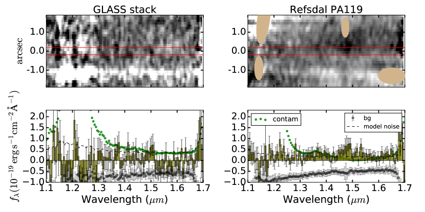
Figure A1.— Top: Contamination-subtracted two-dimensional grism spectra from the two GLASS (left) and single Refsdal P.A. $=119^{\circ}$ (right) position angles. As in Figure 3, black represents positive signal and the 2D spectra were smoothed with a 2D Gaussian kernel with $\mathrm{FWHM}=2$ pixels in both dimensions. Bottom: One-dimensional extractions (yellow histogram) of the two-dimensional spectra above. The bulk of the signal comes from the deeper Refsdal data, as expected for a real signal. The strong negative residual at $\sim-1.2$ arcsec in the GLASS stack comes almost entirely from the GLASS P.A. $=32^{\circ}$. This residual is down-weighted in Figure 3 when making the stack. While in principle the signal should taper at $\lambda\geq 1.65~{}\mu m$ due to the declining throughput of G141, contamination is severe in both cases at these wavelengths, making this test uninformative.

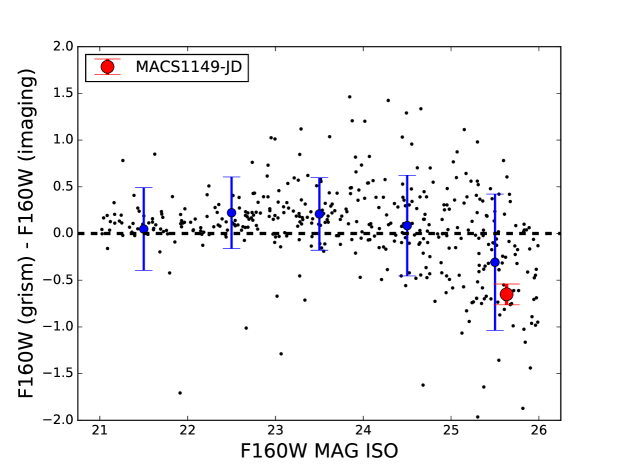
Figure A2.— Comparison of magnitudes calculated from the grism and from the photometry over the HST F160W bandpass for 425 individual objects (black points) in the grism field of view. The blue points and error bars represent the mean and standard deviation of the points in equally spaced bins that are 1 magnitude wide. The magnitude offset for MACS1149-JD is shown in red, consistent with the offsets observed for similarly faint objects.

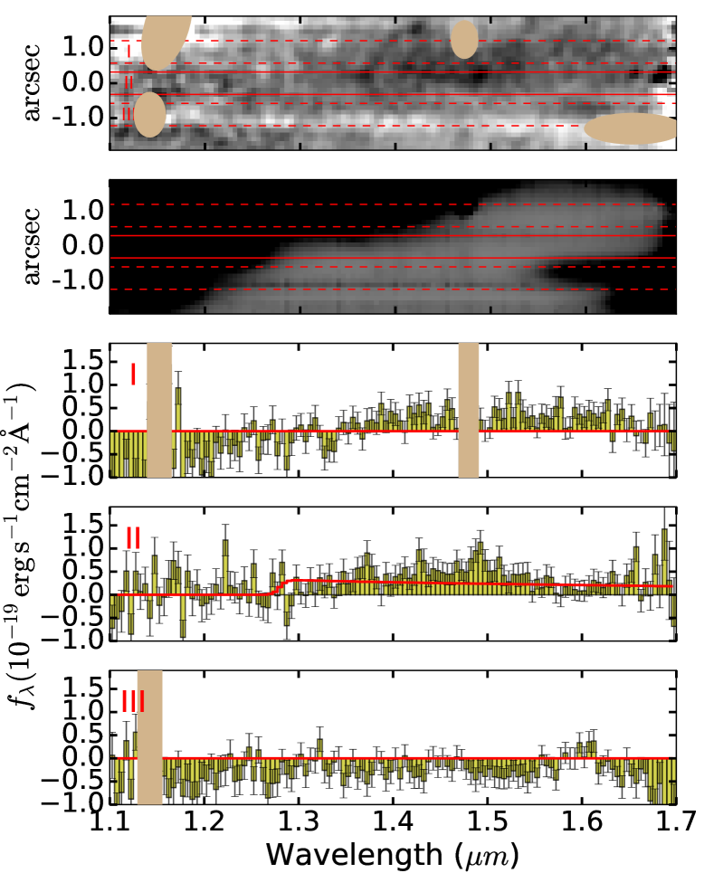
Figure A3.— Drizzled two-dimensional spectrum (top), contamination model (second row), and one-dimensional extractions at three different vertical extraction apertures from the combination of the two GLASS P.A.s and the Refsdal P.A. $=119^{\circ}$ data. The top spectrum was smoothed with a 2D Gaussian kernel with $\mathrm{FWHM}=2$ pixels in both dimensions. The spatial apertures (I, II and III) are chosen so that the flux from MACS1149-JD predicted from HST F160W falls within the central (II) aperture only. Contamination residuals are strong everywhere except the central aperture where the trace from MACS1149-JD is expected.

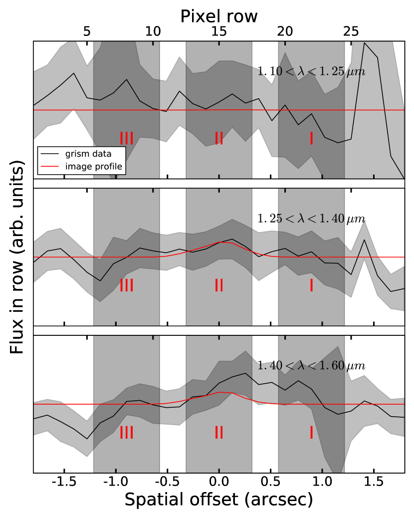
Figure A4.— The spatial profile extracted from the Refsdal P.A. $=119^{\circ}$ spectrum of MACS1149-JD. The three panels show the spatial extraction in three separate wavelength intervals: top: $1.10<\lambda<1.25~{}\mu m$, middle: $1.25<\lambda<1.40~{}\mu m$, bottom: $1.40<\lambda<1.60~{}\mu m$. In all three panels, the black line and dark gray region represent the mean and standard deviation, respectively, of the flux in each spatial row of the two-dimensional spectrum. The red line indicates the spatial profile extracted from a LBG model fixed to the best-fit grism redshift, $z=9.53$, whose morphology and magnitude are determined by the HST F160W image. The three spatial regions from Figure A3 are shown on each panel with shaded vertical regions. Reassuringly, the data show a peak in flux in the central region (region II) for the two redder wavelength bins, but not in the bluer bin, consistent with the expectation from the model. Residual contamination is likely responsible for the excess flux in the bottom panel at positive spatial offsets.

References

- Ageorges et al. (2010) Ageorges, N., Seifert, W., Jütte, M., et al. 2010, in Proc. SPIE, Vol. 7735, Ground-based and Airborne Instrumentation for Astronomy III, 77351L
- Anders & Fritze-v. Alvensleben (2003) Anders, P., & Fritze-v. Alvensleben, U. 2003, A&A, 401, 1063
- Bertin & Arnouts (1996) Bertin, E., & Arnouts, S. 1996, A&AS, 117, 393
- Bian et al. (2015) Bian, F., Stark, D. P., Fan, X., et al. 2015, ApJ, 806, 108
- Bouwens et al. (2014) Bouwens, R. J., Illingworth, G. D., Oesch, P. A., et al. 2014, ApJ, 793, 115
- Bouwens et al. (2015) —. 2015, ApJ, 803, 34
- Bradač et al. (2005) Bradač, M., Schneider, P., Lombardi, M., & Erben, T. 2005, A&A, 437, 39
- Bradač et al. (2009) Bradač, M., Treu, T., Applegate, D., et al. 2009, ApJ, 706, 1201
- Bradač et al. (2014) Bradač, M., Ryan, R., Casertano, S., et al. 2014, ApJ, 785, 108
- Brammer (2016) Brammer, G. 2016, Reprocessing WFC3/IR Exposures Affected by Time-Variable Backgrounds, Tech. rep.
- Brammer et al. (2014) Brammer, G., Pirzkal, N., McCullough, P., & MacKenty, J. 2014, Time-varying Excess Earth-glow Backgrounds in the WFC3/IR Channel, Tech. rep.
- Brammer et al. (2008) Brammer, G. B., van Dokkum, P. G., & Coppi, P. 2008, ApJ, 686, 1503
- Brammer et al. (2012) Brammer, G. B., van Dokkum, P. G., Franx, M., et al. 2012, ApJS, 200, 13
- Brammer et al. (2016) Brammer, G. B., Marchesini, D., Labbé, I., et al. 2016, ApJS, 226, 6
- Bruzual & Charlot (2003) Bruzual, G., & Charlot, S. 2003, MNRAS, 344, 1000
- Calzetti et al. (2000) Calzetti, D., Armus, L., Bohlin, R. C., et al. 2000, ApJ, 533, 682
- Castellano et al. (2016) Castellano, M., Amorín, R., Merlin, E., et al. 2016, A&A, 590, A31
- Castellano et al. (2017) Castellano, M., Pentericci, L., Fontana, A., et al. 2017, ApJ, 839, 73
- Chabrier (2003) Chabrier, G. 2003, PASP, 115, 763
- Conroy & van Dokkum (2012) Conroy, C., & van Dokkum, P. G. 2012, ApJ, 760, 71
- de Barros et al. (2014) de Barros, S., Schaerer, D., & Stark, D. P. 2014, A&A, 563, A81
- Di Criscienzo et al. (2017) Di Criscienzo, M., Merlin, E., Castellano, M., et al. 2017, ArXiv e-prints, arXiv:1706.03790
- Ebeling et al. (2001) Ebeling, H., Edge, A. C., & Henry, J. P. 2001, ApJ, 553, 668
- Egami et al. (2005) Egami, E., Kneib, J.-P., Rieke, G. H., et al. 2005, ApJ, 618, L5
- Erb et al. (2010) Erb, D. K., Pettini, M., Shapley, A. E., et al. 2010, ApJ, 719, 1168
- Foreman-Mackey et al. (2013) Foreman-Mackey, D., Hogg, D. W., Lang, D., & Goodman, J. 2013, PASP, 125, 306
- Gonzaga et al. (2012) Gonzaga, S., Hack, W., Fruchter, A., & Mack, J. 2012, The DrizzlePac Handbook
- Greig & Mesinger (2017) Greig, B., & Mesinger, A. 2017, ArXiv e-prints, arXiv:1705.03471
- Henry et al. (2015) Henry, A., Scarlata, C., Martin, C. L., & Erb, D. 2015, ApJ, 809, 19
- Hill et al. (2012) Hill, J. M., Green, R. F., Ashby, D. S., et al. 2012, in Proc. SPIE, Vol. 8444, Ground-based and Airborne Telescopes IV, 84441A
- Holden et al. (2016) Holden, B. P., Oesch, P. A., González, V. G., et al. 2016, ApJ, 820, 73
- Horne (1986) Horne, K. 1986, PASP, 98, 609
- Huang et al. (2016) Huang, K.-H., Bradač, M., Lemaux, B. C., et al. 2016, ApJ, 817, 11
- Kawamata et al. (2016) Kawamata, R., Oguri, M., Ishigaki, M., Shimasaku, K., & Ouchi, M. 2016, ApJ, 819, 114
- Kelly et al. (2015) Kelly, P. L., Rodney, S. A., Treu, T., et al. 2015, Science, 347, 1123
- Kelly et al. (2016) Kelly, P. L., Brammer, G., Selsing, J., et al. 2016, ApJ, 831, 205
- Labbé et al. (2013) Labbé, I., Oesch, P. A., Bouwens, R. J., et al. 2013, ApJ, 777, L19
- Laporte et al. (2017) Laporte, N., Ellis, R. S., Boone, F., et al. 2017, ApJ, 837, L21
- Leitherer & Heckman (1995) Leitherer, C., & Heckman, T. M. 1995, ApJS, 96, 9
- Lotz et al. (2016) Lotz, J. M., Koekemoer, A., Coe, D., et al. 2016, ArXiv e-prints, arXiv:1605.06567
- Mason et al. (2017) Mason, C. A., Treu, T., Dijkstra, M., et al. 2017, ArXiv e-prints, arXiv:1709.05356
- Merlin et al. (2016) Merlin, E., Amorín, R., Castellano, M., et al. 2016, A&A, 590, A30
- Mesinger et al. (2015) Mesinger, A., Aykutalp, A., Vanzella, E., et al. 2015, MNRAS, 446, 566
- Mesinger et al. (2016) Mesinger, A., Greig, B., & Sobacchi, E. 2016, MNRAS, 459, 2342
- Oesch et al. (2016) Oesch, P. A., Brammer, G., van Dokkum, P. G., et al. 2016, ApJ, 819, 129
- Pentericci et al. (2011) Pentericci, L., Fontana, A., Vanzella, E., et al. 2011, ApJ, 743, 132
- Pentericci et al. (2014) Pentericci, L., Vanzella, E., Fontana, A., et al. 2014, ApJ, 793, 113
- Planck Collaboration et al. (2016) Planck Collaboration, Adam, R., Aghanim, N., et al. 2016, A&A, 596, A108
- Richard et al. (2011) Richard, J., Kneib, J.-P., Ebeling, H., et al. 2011, MNRAS, 414, L31
- Schaerer & de Barros (2009) Schaerer, D., & de Barros, S. 2009, A&A, 502, 423
- Schenker et al. (2012) Schenker, M. A., Stark, D. P., Ellis, R. S., et al. 2012, ApJ, 744, 179
- Schmidt et al. (2014) Schmidt, K. B., Treu, T., Brammer, G. B., et al. 2014, The Astrophysical Journal Letters, 782, L36
- Schmidt et al. (2016) Schmidt, K. B., Treu, T., Bradač, M., et al. 2016, ApJ, 818, 38
- Senchyna et al. (2017) Senchyna, P., Stark, D. P., Vidal-García, A., et al. 2017, ArXiv e-prints, arXiv:1706.00881
- Shim et al. (2011) Shim, H., Chary, R.-R., Dickinson, M., et al. 2011, ApJ, 738, 69
- Smit et al. (2014) Smit, R., Bouwens, R. J., Labbé, I., et al. 2014, ApJ, 784, 58
- Smith et al. (2009) Smith, G. P., Ebeling, H., Limousin, M., et al. 2009, ApJ, 707, L163
- Stark (2016) Stark, D. P. 2016, ARA&A, 54, 761
- Stark et al. (2015) Stark, D. P., Walth, G., Charlot, S., et al. 2015, MNRAS, 454, 1393
- Trenti et al. (2015) Trenti, M., Perna, R., & Jimenez, R. 2015, ApJ, 802, 103
- Treu et al. (2013) Treu, T., Schmidt, K. B., Trenti, M., Bradley, L. D., & Stiavelli, M. 2013, ApJ, 775, L29
- Treu et al. (2015) Treu, T., Schmidt, K. B., Brammer, G. B., et al. 2015, ApJ, 812, 114
- Treu et al. (2016) Treu, T., Brammer, G., Diego, J. M., et al. 2016, ApJ, 817, 60
- Zheng et al. (2012) Zheng, W., Postman, M., Zitrin, A., et al. 2012, Nature, 489, 406
- Zheng et al. (2017) Zheng, W., Zitrin, A., Infante, L., et al. 2017, ApJ, 836, 210
- Zitrin & Broadhurst (2009) Zitrin, A., & Broadhurst, T. 2009, ApJ, 703, L132
- Zitrin et al. (2015a) Zitrin, A., Ellis, R. S., Belli, S., & Stark, D. P. 2015a, ApJ, 805, L7
- Zitrin et al. (2015b) Zitrin, A., Labbé, I., Belli, S., et al. 2015b, ApJ, 810, L12