Mapping diffuse interstellar bands in the local ISM on small scales via MUSE 3D spectroscopy

Abstract

Context. We map the interstellar medium (ISM) including the diffuse interstellar bands (DIBs) in absorption toward the globular cluster NGC 6397 using VLT/MUSE. Assuming the absorbers are located at the rim of the Local Bubble we trace structures on the order of mpc (milliparsec, a few thousand AU).

Aims. We aimed to demonstrate the feasibility to map variations of DIBs on small scales with MUSE. The sightlines defined by binned stellar spectra are separated by only a few arcseconds and we probe the absorption within a physically connected region.

Methods. This analysis utilized the fitting residuals of individual stellar spectra of NGC 6397 member stars by Husser et al. (2016) and Kamann et al. (2016) and analyzed lines from neutral species and several DIBs in Voronoi-binned composite spectra with high signal-to-noise ratio (S/N).

Results. This pilot study demonstrates the power of MUSE for mapping the local ISM on very small scales which provides a new window for ISM observations.

We detect small scale variations in $\rm Na\,{\scriptstyle I}$ and $\rm K\,{\scriptstyle I}$ as well as in several DIBs within few arcseconds, or mpc with regard to the Local Bubble. We verify the suitability of the MUSE 3D spectrograph for such measurements and gain new insights by probing a single physical absorber with multiple sight lines.

1 Introduction

Systematic studies of the interstellar medium (ISM) are of prime importance to understanding the life-cycle of baryons in the Universe and the evolution of galaxies. Because the ISM spans several orders of magnitudes in gas densities and temperatures and is structured down to AU scales, our understanding of the ISM is still quite limited.

Among the various different methods of studying the ISM, absorption spectroscopy in the ultraviolet (UV) and optical regime has become a particularly powerful approach to explore the ISM’s chemical composition, kinematics, and spatial structure. Not long after the first detection of interstellar absorption lines in the Ca H & K lines (Hartmann 1904) a number of broad optical absorption features of unknown origin were discovered (Heger 1922). These features were given the name diffuse interstellar bands (DIBs). Today, more than 400 DIBs have been identified in the Milky Way’s ISM (Herbig 1995; Sarre 2006) and they have also been observed in other galaxies (e.g., in the Magellanic Clouds; Walker 1963; Ehrenfreund et al. 2002 or even beyond the local group by Monreal-Ibero et al. 2015b). Even almost 100 years after their first detection, however, the exact origin of the DIBs (i.e., their carriers) is largely uncertain. One preferred scenario is, that DIBs represent carbon-based molecular structures and possibly are related to polycyclic aromatic hydrocarbons (PAHs; e.g., Crawford et al. 1985, Cox 2011). The strengths of the various DIBs show a rather complex behavior when compared to other tracers of interstellar gas and dust particles, such as the color excess $E(B-V)$ and the equivalent width of neutral and molecular species (e.g., Na i, CN). This indicates that the DIB carriers are different from those of interstellar dust particles and simple molecules (e.g., Friedman et al. 2011). Despite the uncertain origin, DIBs can be used as a diagnostic tool to study the radiation field and gas temperature in the ISM (Cami et al. 1997; Vos et al. 2011). And, if multiple sightlines at small angular separations are used, DIBs do serve as tracer species to study the small-scale structure in the ISM (van Loon et al. 2009, van Loon et al. 2013; Cordiner et al. 2013). The large number of different DIBs and their commonness render the nature of DIBs a pressing puzzle.

Andrews et al. (2001) and van Loon et al. (2009) present indications for small scale structures in the ISM in individual sightlines toward globular cluster stars on parsec scale, while Smith et al. (2013) and Boissé et al. (2013) tested for spatial variations on even smaller scales utilizing the proper motion of stars and the implied drift of the line of sight through the foreground gas.

The existence of small regions with comparably high density within the diffuse ISM has important implications for interstellar chemistry. Their detection might also provide a potential method for obtaining new information on the physical conditions, and a possible solution to some of the challenges which exist in reproducing the abundances of molecules observed along lines of sight through the diffuse ISM (Smith et al. 2013). Andrews et al. (2001) point out that fluctuations in ionization equilibrium and not just total column density may be responsible for the observed variations in the ISM on small scales. It appears to be essential to take the spatial information into account for the quest to understand the nature of the DIBs as well as their carriers. While, for example, Monreal-Ibero et al. (2015) trace the extinction on the plane of the sky and deepen the knowledge on the DIB correlations with dust, works like van Loon et al. (2015) provide further strong evidence that the origin of the DIBs is manifold and they do indeed show structures on small scales, which help to differentiate between them. Despite the number of detections, the nature of these structures and their ubiquity is still a subject of study. It has not always been clear whether they reflect the variation in $\rm H\,{\scriptstyle I}$ column density, or whether they are caused by changes in the physical conditions of the gas over small scales.

In this paper we take advantage of the manifold capabilities of the Multi Unit Spectroscopic Explorer (MUSE) installed at the ESO Very Large Telescope (VLT) to study DIBs and optical absorption lines in the local ISM at very small angular scales in the direction of the globular cluster NGC 6397 in the broad wavelength range between 4650Å  and 9300Å. The MUSE 3D spectrograph provides a respectable FOV of $1^{\prime}\times 1^{\prime}$ and a spatial sampling of $0.2^{\prime\prime}\times 0.2^{\prime\prime}$ which enables us to construct equivalent width maps of DIBs and of their correlation with respect to each other or with the observed ISM features for a physically connected region. DIBs that are related to the same carrier should reveal themselves in similar 2D maps. With the high spatial resolution we trace the correlation between DIBs within connected regions which can disclose the preferred environment of individual DIBs.

In Sect. 2 we describe the MUSE observations and several ancillary data taken with other instruments. Section 3 depicts the applied method to obtain information on the ISM absorption features from the MUSE data cubes and the results are presented in Sect. 4. We discuss the new findings and its implications in Sect. 5. Further plots and details on the fitting procedure can be found in the Appendix.Throughout the paper the wavelengths $\lambda$ is given in Å, e.g., $\rm K\,{\scriptstyle I}$ 7664, DIB 5780, and equivalent widths in mÅ, unless noted otherwise.

2 The data

NGC 6397 is the second closest globular cluster with a distance of merely 2.3 kpc and a reddening of E(B-V) = 0.18 (Harris 2010). At a galactic latitude of -11.06^∘ and longitude of +338.17^∘, the globular cluster (GC) sits below the Galactic disk at about 6 kpc distance to the Galactic center. The GC has a mean radial velocity of $v_{\mathrm{rad}}=17.84\pm 0.07$$\mathrm{\mathrm{\ km}\mathrm{\ s}^{-1}}$(see Husser et al. 2016, hereafter referred to as Paper I). NGC 6397 is often considered to be one of the 20 globulars (at least) in our Milky Way Galaxy that have undergone a core collapse. Core collapse is when a globular’s core has contracted to a very dense stellar agglomeration (see Kamann et al. 2016, hereafter referred to as Paper II).

2.1 The MUSE data

NGC 6397 was observed during MUSE commissioning, lasting from July 26nd to August 3rd, 2014. 23 MUSE pointings were arranged in a $5\times 5$ mosaic with two missing frames, covering roughly $300^{\prime}\times 300^{\prime}$ on the sky. The exposure times ranged from 25s to 60s per individual observation, accumulating about 4 min per pointing on average. This limitation was set to avoid saturation effects of the brightest cluster giants as the original studies in Papers I & II focused on the stars themselves. In total, we obtained 127 exposures with a total integration time of 95 min. Including overheads, the observations took about 6 h. While the seeing varied below $1^{\prime\prime}$, the central pointings were recorded at a seeing of $0.6^{\prime\prime}$. The data reduction was done using the official MUSE pipeline (in versions 0.18.1, 0.92, and 1.0) described in Weilbacher et al. (2012). See Paper I for detailed information on the MUSE observations of NGC 6397. The resolving power of the MUSE instrument ranges from $\sim 2000$ at 4650Å  to $\sim 4000$ at 9300Å. The data consists of roughly 19,000 spectra of $\sim$ 12,000 individual stars. Even at a resolution of $\approx 100$ $\mathrm{\mathrm{\ km}\mathrm{\ s}^{-1}}$, most of the strong DIBs are resolved, due to their eponymous broad profiles. However, we are strictly limited by the resolution of our data with regard to resolving individual velocity components in the narrow absorption lines of neutral species such as $\rm K\,{\scriptstyle I}$   or the $\rm Na\,{\scriptstyle I\,D}$   doublet.

The observed field is strongly dominated by cluster member stars. We expected comparably few foreground stars toward the position of NGC 6397 below the Galactic disk. For an adjacent field of the same angular size, the GAIA archive of Data Release 1 contains $\approx$ 100 stars brighter than 18th magnitude (see Gaia Collaboration 2016, Fabricius et al. 2016). 18th magnitude stars correspond to a S/N of approximately ten which we used as lower threshold in our sample. As will be discussed in Sect. 5.2 there is strong evidence that the absorbing cloud is nearby but even if those $\approx$ 100 stars were distributed highly inhomogeneously across the field, they would not impact the results. Each spatial measurement was based on more than 300 stars (see Sect. 3.2).

In Fig. 1 we plot all stars relative to the cluster center. The individual pointings are indicated.

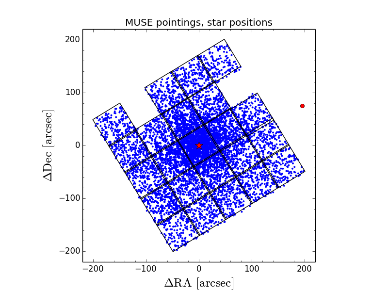
Figure 1: Area covered by our observations: black: MUSE pointings, blue: individual stellar positions, red circle: Single High resolution UVES pointing relative to the center of NGC 6397 (red star).

2.2 Ancillary data

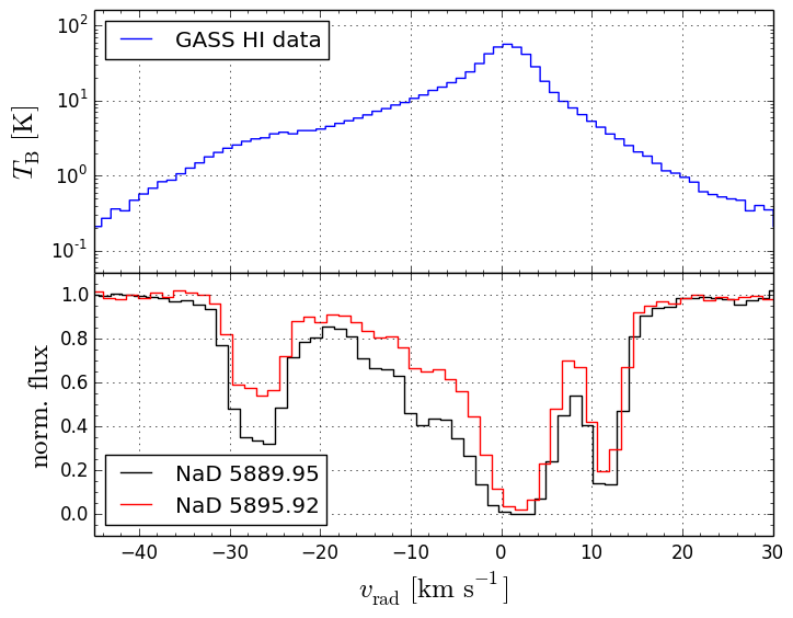
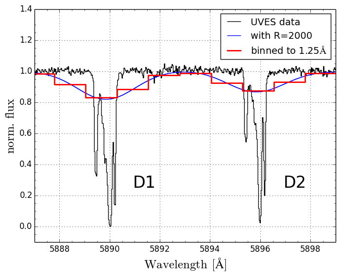
Figure 2: top panel:UVES spectrum of $\rm Na\,{\scriptstyle I\,D}$ doublet + $\rm H\,{\scriptstyle I}$ GASS data (blue), bottom panel:UVES spectrum of $\rm Na\,{\scriptstyle I\,D}$ doublet D1 and D2 (black), convolved to MUSE resolution (blue) and binned to default MUSE sampling of 1.25Å  (red). The scale for all data is helio-centric.

2.2.1 UVES data

We used a high resolution spectrum from VLT/UVES in the direction of NGC 6397 of one of its cluster members to verify the results we derived from low resolution MUSE data and to provide a reference spectrum for interstellar absorption. A marker in Fig. 1, about 200 arcsecs from the cluster center, reflects the position of star NGC 6397-T183. This star lies outside of our map and also outside of the cluster’s core region, but since it is relatively close on the sky, its spectrum should give useful indications on the velocity components present in this direction. We retrieved a high resolution UVES spectrum from the ESO archive. At a slit width of $0.3^{\prime\prime}$, the UVES spectrum has a resolution of $R\approx 115,000$ and a S/N of $\sim$ 50. The UVES data for the nearby B-Type star in the top panel of Fig. 2 reveal three components. At $v_{\mathrm{helio}}\approx$ -26 $\mathrm{\mathrm{\ km}\mathrm{\ s}^{-1}}$, the main saturated component at rest and the stellar component at $\approx$ +12 $\mathrm{\mathrm{\ km}\mathrm{\ s}^{-1}}$for this individual star. There is a weak fourth component at $\approx$ -10 $\mathrm{\mathrm{\ km}\mathrm{\ s}^{-1}}$.

The wavelength region around the $\rm Na\,{\scriptstyle I\,D}$ absorption for this individual cluster star is shown in Fig. 2. A comparison of these data at their original resolution and once degraded to the MUSE spectral resolution is illustrated. The plot shows the same region of the UVES data in wavelength space. The resulting spectrum after a convolution with a Gaussian kernel to the MUSE resolution of $R\approx 2,200$ at the given wavelength is also shown, as are the 1.25Å  sampling of the MUSE data as present in the MUSE pipeline-reduced data cubes. In addition to $\rm Na\,{\scriptstyle I\,D}$ , only DIB 5780 and DIB 6283 are covered in the high resolution data (see Sect. 5).

The analysis presented in this paper is solely based on the MUSE data, with exceptions indicated in the text. We note that the stellar component (as well as the unresolved telluric absorption component) will be removed prior to data analysis as described in Sect. 3. The findings based on the UVES data are further discussed in Sect. 5.1.

2.2.2 GASS data on $\rm H\,{\scriptstyle I}$ 

To further study the gas kinematics of the neutral ISM toward NGC 6397 (including the more diffuse warm neutral phase that is not traced by Na i absorption) we used publicly available H i 21cm data from the Galactic-All Sky Survey (GASS; McClure-Griffiths et al. 2009; Kalberla et al. 2010; see https://www.astro.uni-bonn.de/hisurvey). The GASS survey was carried out with the 64m radio telescope at Parkes. The spectral resolution is $0.82$ km s^-1 at an rms of $57$ mK per spectral channel ($\Delta v=0.8$ km s^-1), while the beam size of the data is $\sim 16\arcmin$, thus providing a rough estimate of $N(\rm H\,{\scriptstyle I}\,)$ as the effective FWHM of the beam is larger than the MUSE FOVs.

If one assumes that the gas is optically thin, the column density of $\rm H\,{\scriptstyle I}$ can then be obtained from the brightness temperature $T(v)$ per velocity bin from the GASS data:

$$N_{\mathrm{H}}=1.82\times 10^{13}\int T(v)\,dv\,\,\,\mathrm{atoms\,cm}^{-2},$$ (1)

leading to a total column density of $\log[N(\rm H\,{\scriptstyle I}\,)]=21.1$. As this is observed in emission, gas beyond NGC 6397 could contribute to the total budget. The low galactic latitude of -11.06^∘ for NGC 6397 suggests that all observed $\rm H\,{\scriptstyle I}$  is in the foreground of the GC.

The 21cm brightness temperature profile toward NGC 6397 is shown in the top panel in Fig. 2. The radio data clearly displays the main component at rest as well as the much weaker blue shifted component at $v_{\rm helio}=-26$ km s^-1.

2.2.3 Extinction data

The reddening E(B-V) toward NGC 6397 is given as 0.18 in Harris (2010) and only varies between 0.185 and 0.191 across the MUSE mosaic (see extinction map data from Schlegel et al. 1998, who combined results of IRAS and COBE/DIRBE).

The resolution of the available E(B-V) data is too low and would conceal possible structures on smaller scales but could indicate a large scale gradient across the FOV which is not the case here.

3 Extraction of absorption features in MUSE spectra

3.1 Modeling of the stellar population and telluric correction

Each of the stellar spectra were PSF-extracted simultaneously from the single data cubes. The process is described and successfully applied in Paper I.

In Paper I every extracted stellar spectrum of the globular cluster was fitted with a template spectrum based on PHOENIX models. The stellar templates were scaled with a polynomial as linear fit to account for reddening and hypothetical flux calibration inconsistencies in the commissioning data. Furthermore, an individual telluric model was fitted to each spectrum, though we expect a rather homogeneous sky background for each MUSE field of view. Paper I describes this process in great detail. The telluric absorption lines were fitted with models of varying H₂O  and O₂/O₃  abundances (Husser & Ulbrich 2014). This work utilizes the residuals of the above mentioned template matching and sky fitting procedures. Once the stellar templates and telluric absorption lines are subtracted, the only features that remain are hypothetical stellar lines not represented in the models, potential misfits of stellar templates, and absorption features of the interstellar medium along the line of sight toward NGC 6397.

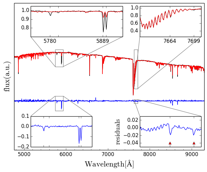
Figure 3: Steps of data processing. In black the data for one of the brightest stars in the field with a S/N $\sim$ 120. In red the best fit to the data including the telluric absorption line fit as well. In blue below the fitting residuals to scale with the plotted spectrum. The enlargement windows to the left, highlight the region around the DIBs 5780,5797 and the $\rm Na\,{\scriptstyle I\,D}$ doublet. On the right hand side, the zoom illustrates the success of the telluric absorption line fit. We note that the zoom into the fitting residuals for this region is scaled by a factor of 10. For this example based on a single star of particularly high S/N, the $\rm K\,{\scriptstyle I}$ doublet stands out even for an individual stellar fit (red triangles).

As a first iteration, a subset of the 19,000 spectra was selected based on a S/N threshold and a minimum stellar temperature.

The temperature threshold was conservatively set to 4,000K. Colder stars begin to show strong molecular features and unresolved bands and it is practically impossible to get a reliable estimate of the local continuum. For the final analysis, all stars with a S/N ¡ 10 were excluded as their stellar template matching lacks the precision to derive meaningful information from the residuals at the required level. That final sample contains 9,746 spectra.

Figure 3 illustrates the reduction process for an individual star. The best template match is plotted on top of the observed data. The method applied to fit the stellar templates does not provide a stellar continuum model. From the perspective of the interstellar matter along the line of sight, however, the stellar flux itself represents the continuum level and the residuals from the stellar fitting were then scaled with the final stellar template. The resulting continuum spectrum is also shown. After this step, the residuals range from 0, the former stellar flux, to -1, meaning 100% of the stellar flux was absorbed. This is illustrated in Fig. 3 in the bottom left and right insets. After adding an offset of one the processed residual spectrum has the same properties as a normalized absorption spectrum.

3.2 Improving S/N by tessellation

For the general analysis, the individual residual-spectra, were co-added with error weighting into Voronoi bins of equal S/N. The applied Voronoi algorithm is based on the procedure presented in Cappellari & Copin (2003).

Voronoi binning is a special kind of tessellation that solves the problem of preserving the maximum spatial resolution of general two-dimensional data, given a constraint on the minimum S/N. This automatically leads to somewhat homogeneous S/N per bin with varying bin-sizes. The uneven spacing of the stars as well as the strong variation in brightness of neighboring stars leads to varying shapes (but always convex) of the individual bins.

As each spectrum was extracted from the 23 MUSE data cubes which were reduced to the same wavelength grid, no re-sampling of the individual spectra was required for this step.

Our tessellation results in a bin size and thus a resolution which is coupled to the globular cluster via its star density. When using a fixed grid across the FOV, we would couple the star count per bin to the underlying cluster and thereby correlating the error per bin to the stellar distribution. As we deem it crucial to minimize any correlation of the stars themselves with the observed ISM we chose the described tessellation.

We aimed for a S/N per bin of $\sim$ 150 which resulted in the 31 independent Voronoi bins. Each bin contains $\sim$ 300 spectra. For a more detailed map of $\rm K\,{\scriptstyle I}$ and DIB 5705 (see Sect. A.2) we realized a tessellation with 107 bins and $\sim$ 100 spectra per bin. The chosen number of spatial bins is the result of a strict trade-off between S/N per bin and spatial resolution. The spatial resolution of this approach for a globular cluster such as NGC 6397 with many resolved stars is merely limited by the S/N of the stellar spectra. The stars themselves are usually less than two arcseconds apart near the cluster core. The 31 bins span about 20 arcseconds on average with equivalent width errors on the order of 8 mÅ  and about 14 mÅ, for the maps with 107 bins and a S/N of $\sim$ 90 per bin. As these uncertainties in equivalent width are mostly a result of template residuals, the true uncertainty per measured individual equivalent width can vary slightly.

3.3 Measuring absorption features

Several of the observable transitions of ISM species as well as DIBs fall into regions of strong sky contamination. Successful modeling of the stellar contributions and the telluric absorption is key to precision measurements of the often quite weak (in the mÅ  range) equivalent widths (see, i.e., Puspitarini et al. 2013 and Monreal-Ibero & Lallement 2017). While studies based on high resolution spectra can aim at modeling telluric absorption lines individually, these absorption bands are not resolved by the MUSE spectrograph. Its great benefit is, however, to measure thousands of spectra simultaneously and thus under the same conditions. The accuracy of the telluric absorption line fit is illustrated in Fig. 4, in which we plot the equivalent width of both $\rm K\,{\scriptstyle I}$ components against each other. The line strengths for each doublet was fitted as a free parameter to use the ratio as sanity check as well as probe for density variations as mentioned in Sect. 4.2.1. $\rm K\,{\scriptstyle I}$ 7664 sits directly on a strong telluric absorption band, while $\rm K\,{\scriptstyle I}$ 7699 is hardly affected by this (see also Fig. 3 and Fig. 13). At an equivalent width of $\approx$ 50 mÅ, both features are extremely weak and seen at the MUSE resolution the absorption lines show a absorption depth of merely 1-2% of the continuum level. We are confident that the fit of the sky model is sufficiently stable and accurate to recover the information on the stellar flux and interstellar absorption in those regions of the spectrum. The inset in Fig. 4 shows the distribution of the slope for 5,000 bootstrap realizations of the dataset quantifying the correlation in a more robust way than the correlation coefficient of 0.91. Details on the fitting procedure for ISM features as well as DIBs are given in the Appendix.

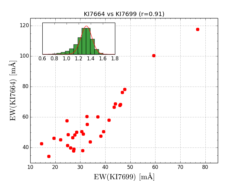
Figure 4: Equivalent widths per bin of $\rm K\,{\scriptstyle I}$ 7664 vs $\rm K\,{\scriptstyle I}$ 7699 for 31 bins. The correlation coefficient is 0.91. The inset in the upper left shows the distribution of the derived slope based on 5,000 bootstrap samples. The Gaussian curve in red corresponds to 1.33 $\pm$ 0.09, though the ratio between the two lines is not constant which is also apparent from the asymmetric distribution.

4 Results on interstellar absorption

4.1 MUSE integrated spectrum

After applying the procedure described in Sect. 3, the former residual data behave like normalized flux spectra cleaned of stellar or telluric absorption line features.

For the identification of ISM features, all stellar spectra were combined into an error-weighted mean single high S/N spectrum. The term signal-to-noise ratio is ambiguous in this context. Interpreting noise as everything that does not contribute to our signal, basically residuals after our ISM and DIB feature fit, we can derive a S/N for the region 5600-5900Å  of $\approx$ 700 based on the standard deviation of the residuals. That S/N also reflects systematic uncertainties in the template matching. Stellar templates are not perfect and not all deviations are normally distributed and scale with $\sqrt{N}\sim 100$. The photon noise itself, as a statistical quantity, is extremely low for our composite spectrum of almost 10,000 stars and the S/N is on the order of 2,000.

The individual spectra were weighted by the square of their S/N. An illustration with an enlargement of the wavelength of the resulting composite spectrum is shown in Fig. 5. The S/N is $\approx$ 700 for the blue part and slightly lower for the red end beyond 7000Å. The equivalent width error due to the measurement uncertainties is $\sigma_{\mathrm{EW}}=\sigma_{\mathrm{flux}}\times\frac{\Delta\lambda}{N_{\mathrm{pix}}}$, where $\sigma_{\mathrm{flux}}$ is the standard deviation for the flux, $N_{\mathrm{pix}}$ is the number of points covering the absorption interval and $\Delta\lambda$ the corresponding wavelength range. For the MUSE sampling this makes a factor of 1/1.25 = 0.8. The equivalent width error turns out to be about 2 mÅ  for a DIB in the observed wavelength range.

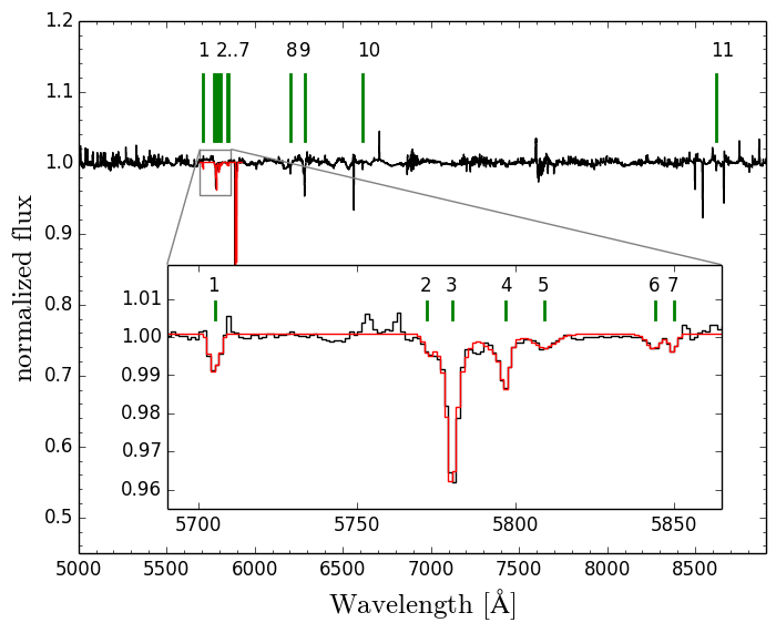
Figure 5: DIBs and $\rm Na\,{\scriptstyle I\,D}$ in the combined residuals for all stellar fits. Namely, DIBs 5705 (1), 5773 (2), 5780 (3), 5797 (4), 5809 (5), 5844 (6), 5850 (7), 6203 (8), 6283 (9), 6613 (10), and 8621 (11). The DIBs are indicated with numbered green lines. The inset shows the DIBs 1-7. The red line is the multi-Gaussian fit for the selected region.

Aside from the $\rm Na\,{\scriptstyle I\,D}$ doublet and the two prominent $\rm K\,{\scriptstyle I}$ lines, numerous DIB features can be identified (see Table 1). Despite the moderate resolution of the MUSE spectrograph of $\sim$ 2,200 - 3,500 in the range of observed DIBs, several DIB features are clearly resolved. The known large intrinsic width of the DIB features surpassing the LSF of MUSE was a motivation to carry out this study with this instrument in the first place.

All identified neutral gas species and DIB features in the composite residual spectrum were fitted as multiple Gaussians with the evolutionary algorithm described in Quast et al. (2005) and applied in Wendt & Molaro (2012). Their positions were fixed to avoid degeneracy with blended features. The equivalent widths were then derived from the modeled Gaussians to account for possible overlap regions. The ISM features in the composite spectrum were fitted with Voigt profiles to derive the column densities. The local continuum was fitted for each group by a low order polynomial. More details on the fitting procedure are provided in the Appendix. For the two $\rm K\,{\scriptstyle I}$ lines as well as the $\rm Na\,{\scriptstyle I\,D}$ doublet the radial velocity was fitted as a common parameter. The broadening parameter of the $\rm K\,{\scriptstyle I}$ doublet was tied for both transitions. The same applies for the $\rm Na\,{\scriptstyle I\,D}$ doublet.

The equivalent widths of the identified DIBs, as well as of the $\rm Na\,{\scriptstyle I}$ and $\rm K\,{\scriptstyle I}$ lines are listed in Table 1. For the combined spectrum the statistical uncertainty of the equivalent widths is on the order of 1-2 mÅ. From the observed brightness temperature of the H i 21cm emission we estimated the total neutral gas column density $\log[N(\rm H\,{\scriptstyle I}\,)]=21.1$ and can compare it to the measured equivalent width of the 5780 DIB for which a phenomenological relation is known.

Table 1: Measured equivalent widths on the combined spectrum. The statistical error is in the order of 1-2 mÅ.

Line-ID	EW [mÅ]	$\log(N)$ [$N$ in cm-2]
DIB 5705	37
DIB 5773	15
DIB 5780	199
DIB 5797	70
DIB 5809	31
DIB 5844	20
DIB 5850	13
DIB 6203	70
DIB 6283	411
DIB 6613	36
DIB 8621	74
$\rm K\,{\scriptstyle I}$ 7664	60
$\rm K\,{\scriptstyle I}$ 7699	38
$\rm K\,{\scriptstyle I}$		11.3
$\rm Na\,{\scriptstyle I}$ 5889	525
$\rm Na\,{\scriptstyle I}$ 5895	411
$\rm Na\,{\scriptstyle I\,D}$		12.5
$\rm H\,{\scriptstyle I}$ (main)		21.1
$\rm H\,{\scriptstyle I}$ (at -21$\mathrm{\mathrm{\ km}\mathrm{\ s}^{-1}}$)		19.9

Thorburn et al. (2003) conclude, that DIB 5780 is not likely to be saturated for equivalent widths below 800mÅ, which is the case for our sight line. Then the galactic relationship (i.e., Friedman et al. 2011) can be applied and it provides the estimate of $\log[\frac{N(\rm H\,{\scriptstyle I}\,)}{\mathrm{cm}^{-2}}]=19.05+0.92\times\log[\frac{W5780}{\mathrm{m\AA}}]$ corresponding to $\log[N(\rm H\,{\scriptstyle I}\,)]=21.16$ based on the DIB measurement alone, which is in very good agreement with our direct measurement of $\rm H\,{\scriptstyle I}$ . Fitting the $\rm H\,{\scriptstyle I}$ emission with multiple Gaussians allows an estimate of $\log[N(\rm H\,{\scriptstyle I}\,)]=19.9$ for the small component at $v_{\mathrm{helio}}\approx$ -21 $\mathrm{\mathrm{\ km}\mathrm{\ s}^{-1}}$as also listed in the table.

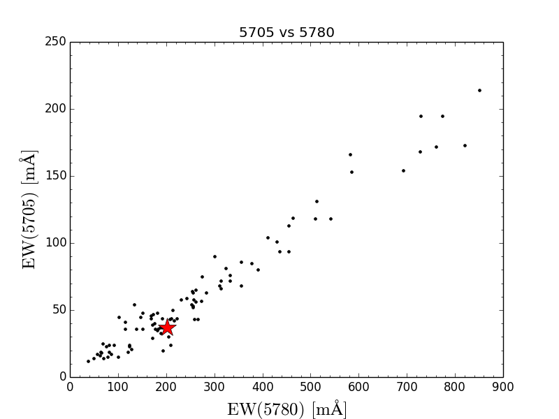
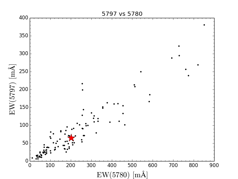
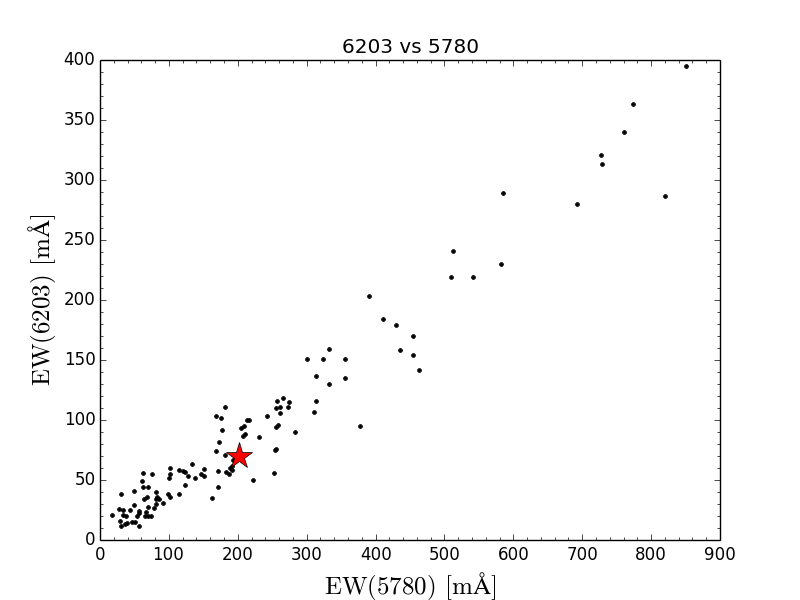
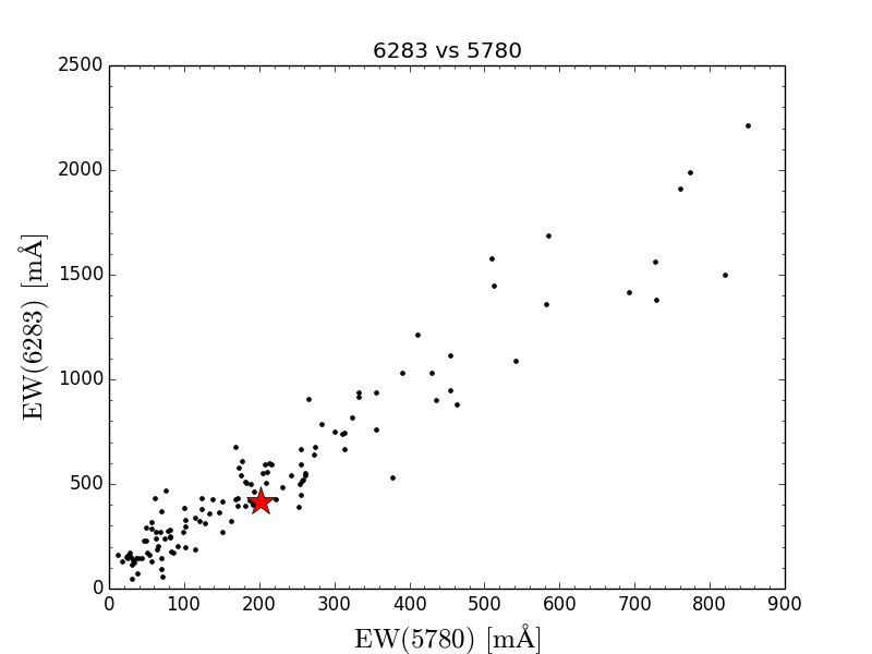
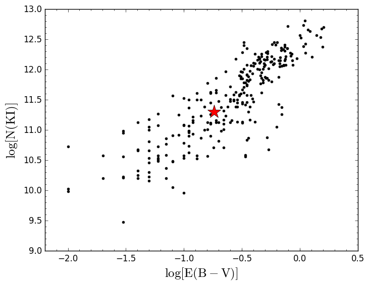
Figure 17: Equivalent widths of DIB 5705, 5797, 6203, 6283 vs DIB 5780 and N($\rm K\,{\scriptstyle I}$ ) vs E(B-V). The black points are data from Friedman et al. (2011), the red star is the measurement based on the composite spectrum.

Figure 6 relates these measurements to those by Welty et al. (2006), Welty & Hobbs (2001) and Friedman et al. (2011) in the Milky Way. The MUSE data allow for excellent measurements of the DIB equivalent widths. The comparison to other DIB data in Fig. 17 further verifies the method utilized here to measure the equivalent widths in composite fitting residuals of cluster stars as the derived absolute equivalent widths for different DIBs lie within the expected correlation to the strong DIB 5780.

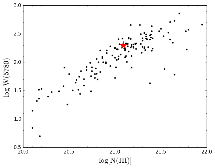
Figure 6: W(5780) vs. N($\rm H\,{\scriptstyle I}$ ). The data for the composite spectrum as listed in Table 1 (red star) overlaid to corresponding data for the Milky Way as published in Welty et al. (2006), Friedman et al. (2011) and Welty & Hobbs (2001) (as scatter plot in black). Measurement uncertainties of those data vary between 3mÅ  and 20mÅ  for DIB 5780 and are omitted here for clarity. For our measurement the statistical error is about 1-2mÅ  and lies within a fraction of the star symbol.

4.2 Spatially resolved $\rm Na\,{\scriptstyle I}$ , $\rm K\,{\scriptstyle I}$ , and DIBs

4.2.1 Maps

In the previous section we saw that the measurements on the composite spectrum of almost 10,000 cluster stars are in very good agreement with other measurements of individual sight lines in the Milky Way. Rather than finding universal correlations between species, we are in the position to be able to probe correlations between DIBs on very small scales and thus likely in a physically connected absorber. Figure 7 shows a spatial map of $\rm Na\,{\scriptstyle I\,D}$ and of the DIB ratio 5780/5797 (this ratio is thought to be sensitive to the UV radiation field: Ensor et al. 2017). The implications are discussed in Sect 4.3. The measured total equivalent width of $\rm Na\,{\scriptstyle I\,D}$ shows no correlation with the brightness of the GC which would otherwise indicate some underlying systematics in the analysis.

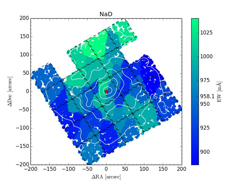
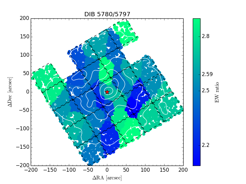
Figure 7: Equivalent width map for the $\rm Na\,{\scriptstyle I\,D}$ doublet (top) and the DIB ratio 5780/5797 (bottom). All selected cluster stars are colored in 31 groups according to their Voronoi-bin. The color reflects the measured total equivalent width of the $\rm Na\,{\scriptstyle I\,D}$ doublet for each composite spectrum per bin with an average of about 960 mÅ. The center of the globular cluster is at coordinate origin and marked with a red star. Brightness contours of the globular cluster are shown as white lines. For the contour plot, the white light image was smoothed to a resolution of 20 arcsec.

Further spatial maps are shown in Fig. 8. The large spatial variations up to a factor of four ($\rm K\,{\scriptstyle I}$ ) or two (DIB 5797) stand out. DIB 6283 shows a distinct anti-correlation to most of the other observed species. Where DIBs 5780, 5797 and $\rm Na\,{\scriptstyle I\,D}$ are strongest, the strength of DIB 6283 drops. This observation is discussed in Sect. 5.5. While the composite equivalent width correlates to the total column density of the gas, the chosen line ratios trace the optical thickness of the gas and it shows well that the abundance of neutral potassium correlates well with that of $\rm Na\,{\scriptstyle I}$ . The equivalent width of the $\rm K\,{\scriptstyle I}$ absorption shows a rather clumpy distribution in Fig. 8 and we prepared maps at higher resolution (at the cost of a drop in S/N) of those absorption features in Fig. 15. It reveals a $\rm K\,{\scriptstyle I}$ region with a size of $40^{\prime\prime}\times 40^{\prime\prime}$. Figure 15 demonstrates that the results in this paper are stable and independent on the specific realization of Voronoi-binning. As expected, the strengths of the absorptions features peaks at higher values for the high resolution, resulting in a slightly higher average equivalent width per bin as well. The given errors represent the statistical variance rather than the uncertainty with respect to the true, potentially unresolved peak of the absorption.

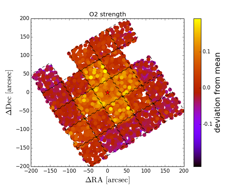
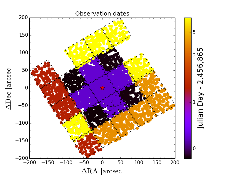
Figure 14: top: Strengths of O₂  in the sky model per individual star with a S/N above 20. bottom: The day of observation relative to JD 2,456,865. The separate pointings are framed in black dashed lines. We note, that several pointings overlap and only the latest visually contributes to this plot.

DIB 5705 appears to have a relatively sharp edge and shows a slightly softer gradient toward the center of the map. The visible structure is not aligned with the individual MUSE pointings on the sky (see Fig. 14 in the Appendix), which would indicate, for example, sky removal problems or other systematics that scale with exposure time or depend on environmental conditions. DIB 5705 and $\rm K\,{\scriptstyle I}$ show the strongest and sharpest variations in equivalent widths within the field of view, although the maximum is not located at the same position for these two tracers. The $\rm Na\,{\scriptstyle I\,D}$ strengths show a filament-like structure and a general gradient which does not coincide spatially with sky background or cluster brightness at all. We consider this further confirmation that the separation of stellar content, telluric absorption lines and interstellar medium was very effective. All visual structures consist of several bins and thus are not dominated by putative peculiar individual stars. These initial results encourage us to perform a more in-depth study based on a larger sample of GC once available.

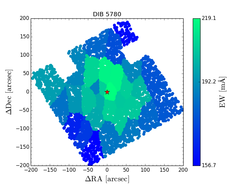
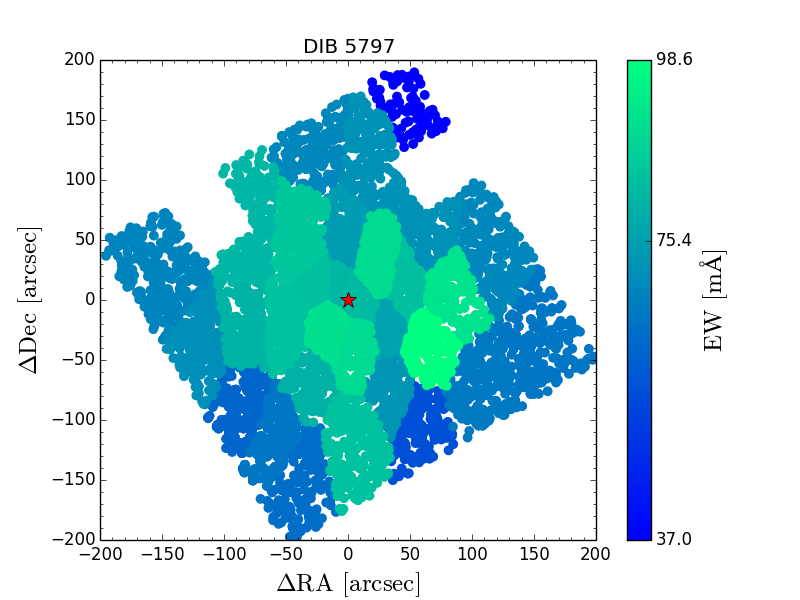
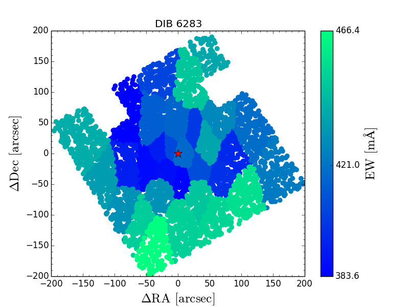
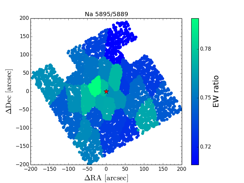
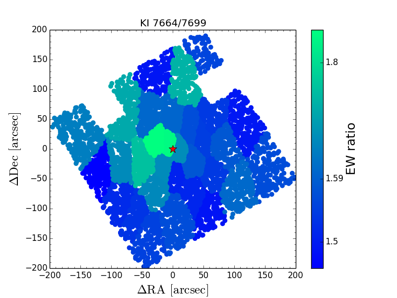
Figure 8: Top: Equivalent width maps with DIBs 5780, 5797; Center: DIB 6283 and $\rm K\,{\scriptstyle I}$ . Bottom: maps of doublet line ratios for $\rm Na\,{\scriptstyle I\,D}$ and $\rm K\,{\scriptstyle I}$ , indicating optical depth. For each map, the $\approx$10,000 selected spectra were combined into 31 Voronoi bins. The color bar shows the equivalent width range as well as the average value for the species. The uncertainty is in the order of 8 mÅ.

4.2.2 Comparison between $\rm Na\,{\scriptstyle I}$ and $\rm K\,{\scriptstyle I}$ absorption

For the 31 bins in Fig. 4, 300 stars (on average) were co-added per bin prior to the EW measurement of the $\rm K\,{\scriptstyle I}$ doublet lines.

These two $\rm K\,{\scriptstyle I}$ features were fitted as independent spectral lines to use them as a qualifier of the telluric correction and to correlate the ratio with other quantities. The $\rm K\,{\scriptstyle I}$ 7664 vs $\rm K\,{\scriptstyle I}$ 7699 ratio is approximately two for optically thin gas, and approaches approximately one for optically thick gas. We observe a range between 1.4 and 1.8. Following Williams (1994), the optical depth $\tau$ of the 7664 Å  line can be calculated from

$$\frac{I_{\mathrm{7664}}}{I_{\mathrm{7699}}}=\frac{1-e^{-\tau}}{1-e^{-\tau/2}}$$ (2)

and considering the lowest equivalent width ratio measured for the $\rm K\,{\scriptstyle I}$ lines to represent their intensities $I_{\mathrm{7664,7699}}$, we derived a value for the optical depth of $\tau\approx 1.8$ for the densest region and a $\tau$ as low as $\approx 0.4$ for the surrounding environment. For the $\rm Na\,{\scriptstyle I\,D}$ ratio a similar rule applies. For optically thin gas, the ratio of the $\rm Na\,{\scriptstyle I\,D}$ doublet 5889/5895 would equal 2.04. The effect on the equivalent widths of $\rm Na\,{\scriptstyle I\,D}$ is much lower as it is mostly saturated already. The measured line ratio ranges between 1.4 and 1.3 (see Fig. 9) and reflect the opacity of the gas. Under the assumption of comparable absorber sizes and a uniform broadening parameter the opacity is proportional to the gas density. Both independent indicators for gas density correlate in our data set as indicated in Fig. 9. They are separated by $\sim$ 1800 Å  and are affected by different atmospheric species. The inset in the upper left shows the distribution of the derived slope based on 5,000 bootstrap samples. The Gaussian fit in red corresponds to 3.5 $\pm$ 1.3. The Spearman’s rank correlation is 0.45. A two-sided hypothesis test whose null hypothesis is that two sets of data are uncorrelated yields a probability of only 0.06 and this scenario thus can be rejected at the 2-$\sigma$ level.

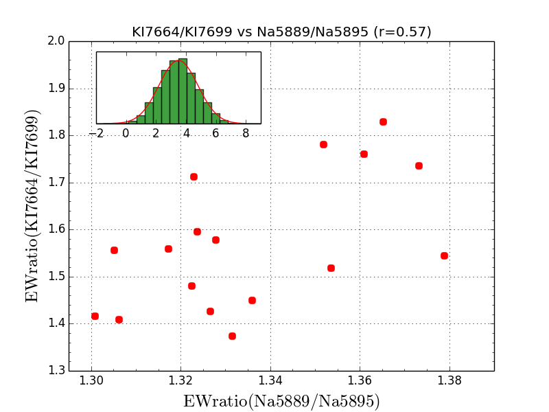
Figure 9: Ratio of $\rm K\,{\scriptstyle I}$ components vs $\rm Na\,{\scriptstyle I\,D}$ components. The inset in the upper-left shows the distribution of the derived slope based on 5,000 bootstrap samples. The Gaussian fit in red corresponds to 3.5 $\pm$ 1.3.

The $\rm K\,{\scriptstyle I}$ doublet probes gas with nearly the same ionization state as $\rm Na\,{\scriptstyle I}$ , but is more likely to be optically thin (the abundance is a factor of about 15 lower than that of $\rm Na\,{\scriptstyle I}$ , while the two doublets have similar oscillator strengths). The ionization potentials of $\rm Na\,{\scriptstyle I}$ and $\rm K\,{\scriptstyle I}$ are only 5.1 eV and 4.3 eV, respectively. These species should primarily probe the $\rm H\,{\scriptstyle I}$   and $\rm H_{\scriptstyle 2}$ ISM phases or represent otherwise non-dominant ionization states in the more diffuse warm neutral gas. Since $\rm K\,{\scriptstyle I}$ and $\rm Na\,{\scriptstyle I}$ have very similar ionization potentials, and show a similar grain depletion pattern (Savage & Sembach 1996), the expected ratio of the $\rm Na\,{\scriptstyle I}$ and $\rm K\,{\scriptstyle I}$ column densities should be $\approx$ 15 for gas with a solar Na/K ratio. For the collapsed spectrum we determine column densities of $\log[N(\rm Na\,{\scriptstyle I}\,)]=12.46$ and $\log[N(\rm K\,{\scriptstyle I}\,)]=11.3$, with a $\rm Na\,{\scriptstyle I}$ /$\rm K\,{\scriptstyle I}$ ratio of 14.5, which is in excellent agreement with the prediction. In Sect. 5.1 we discuss the accuracy to which this ratio can be derived from low resolution MUSE data.

4.3 Comparison of DIBs, $\rm Na\,{\scriptstyle I}$ , and $\rm K\,{\scriptstyle I}$ 

We find a correlation of $\rm K\,{\scriptstyle I}$ 7664/7699 to the DIB 5780/5797 ratio as illustrated in Fig. 10. The correlations in Figs. 9 and 10 are significant according to a Student $t$ test with $t>t_{\mathrm{critical}}$, where $t=r\sqrt{(N-2)/(1-r^{2})}$, with correlation coefficient $r$ and $N$ data points (with in this case $N-2$ degrees of freedom). A bootstrap analysis based on 5,000 samples yields a slope of 0.37 $\pm$ 0.12. The Spearman’s rank correlation is 0.54. A two-sided hypothesis test whose null hypothesis is that two sets of data are uncorrelated yields a probability of only 0.016 and this scenario thus can be safely rejected.

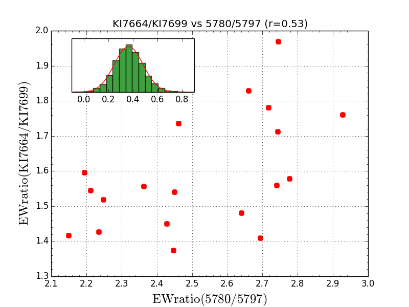
Figure 10: Ratio of $\rm K\,{\scriptstyle I}$ components vs DIB ratio 5780/5797, i.e., ionized/neutral gas. The inset in the upper-left shows the distribution of the derived slope based on 5,000 bootstrap samples. The Gaussian fit in red corresponds to 0.37 $\pm$ 0.12.

According to, for example, Smith et al. (2013) and Vos et al. (2011), the carrier(s) of DIB 5780 do not change ionization easily (it is either already ionized, or neutral and hard to ionize), while DIB 5797 is thought to be caused by a neutral species, easily ionized. Thus, a low DIB 5780/5797 indicates a denser, more shielded region that is less exposed to UV radiation. Ensor et al. (2017) also identify this ratio as a good approximation for the level of UV exposure in their analysis and they find that DIB 5797 itself correlates very well with the overall strengths of DIBs. The correlation of the DIB 5780/5797 ratio with $\rm Na\,{\scriptstyle I}$ opacity is expected but was not yet observed within a single absorbing region. The spatial mapping of the DIB ratio in the bottom panel of Fig. 7 appears to trace a filamentary structure across the field of view. The lowest value of the ratio is in the region that bears the strongest $\rm K\,{\scriptstyle I}$ absorption and highest optical depth. The highest ratios are seen just slightly shifted to the right ($\approx 30$ arcsec) of the filament like structure seen in the $\rm Na\,{\scriptstyle I\,D}$ equivalent maps in Fig. 7. This could indicate some ionizing radiation dominantly from one side (bottom right in the coordinate system used), causing the observed DIB 5780/5797 ratio while the dense regions leftward of this filament are still shielded and less affected.

5 Discussion

We have no direct information on foreground stars, in particular not on individual distances. In Paper I and II, cluster members were identified based on a number of selection criteria. The sample used in this analysis does not consist exclusively of member stars. A comparison with a composite spectrum of likely non-member stars, yielded no significant difference in EW strengths to a members-only selection. This further supports the assumption of the absorber being relatively close. We expect more conclusive distance estimates for some of our other targets. For other globular clusters in our Milky Way, in particular those near the Galactic bulge, the distinction between foreground stars and cluster members will be crucial. Distance measurements by GAIA will contribute greatly to a better understanding of the involved distances for those targets. A more comprehensive interpretation of the new findings will be discussed on the basis of a considerably larger data sample in a follow-up paper that will utilize up to 25 globular cluster targets observed as part of the MUSE guaranteed time observations (PI: S. Dreizler).

5.1 UVES vs MUSE

A conclusive direct comparison of the MUSE data with the single spectrum taken with UVES is not possible since the line of sight toward the individual star lies outside of the mosaic observed with MUSE.

In the single VLT/UVES exposure of NGC 6397-T183 we measure equivalent widths of 85 mÅ  for DIB 5780, and 200 mÅ  for DIB 6283, both modeled with Gaussian functions. These values are considerably lower than for the combined spectrum toward the cluster core that are listed in Table 1 but the line ratio measured in the UVES data agrees very well with the expectation (see Fig. 17, bottom right).

For the UVES spectrum we derived a total column density of $\log[N(\rm Na\,{\scriptstyle I}\,)]=12.6$ based on Voigt profile fits of the three components at $v_{\mathrm{helio}}\approx$ -26 $\mathrm{\mathrm{\ km}\mathrm{\ s}^{-1}}$, -10 $\mathrm{\mathrm{\ km}\mathrm{\ s}^{-1}}$and at rest (see Fig. 2). This matches the prediction given in Ellison et al. (2008) based on the equivalent width of DIB 5780 in galactic sources as well: $\log[\frac{N(\rm Na\,{\scriptstyle I}\,)}{\mathrm{cm}^{-2}}]=10.51+1.1\times\log[\frac{W5780}{\mathrm{m\AA}}]=12.63$.

However, this relation estimates a total column density of $\rm Na\,{\scriptstyle I}$   for the MUSE FOV based on the equivalent width for the combined spectrum of 199 mÅ  for DIB 5780 of $\log[N(\rm Na\,{\scriptstyle I}\,)]=13.04$. The fit to the MUSE data yielded $\log[N(\rm Na\,{\scriptstyle I}\,)]=12.5$, though. While we can measure equivalent widths quite well, we can not expect to obtain accurate results from Voigt profile fits of unresolved absorption features in particular when they are not optically thin, which is indicated by the observed line ratios of the $\rm Na\,{\scriptstyle I\,D}$   doublet. For the combined MUSE data we obtain a ratio of 411mÅ / 525mÅ  = 0.783. The UVES data yields 386mÅ / 511mÅ  = 0.755 indicating a slightly lower optical depth.

The $\rm Na\,{\scriptstyle I}$ /$\rm K\,{\scriptstyle I}$ ratio of 14.5 mentioned in Sect. 4.2.2 thus is critical as fits by Voigt profiles of $\rm K\,{\scriptstyle I}$   and $\rm Na\,{\scriptstyle I}$   lines observed at this low resolution are not expected to provide accurate values for column densities. $\rm Na\,{\scriptstyle I}$ lines are not optically thin and therefore, $N(\rm Na\,{\scriptstyle I}\,)$ is expected to be underestimated; to a lesser extent, this is true also for $N(\rm K\,{\scriptstyle I}\,)$.

5.2 Location and size of the absorbing cloud

The high-resolution UVES spectra as well as the radio data for $\rm H\,{\scriptstyle I}$   indicate that we observe one dominant absorption component toward NGC 6397. The component blueward of the main feature is more than an order of magnitude weaker in $\rm H\,{\scriptstyle I}$ .

Our Sun and nearby stars reside in a region of ionized material referred to as the Local Bubble (Frisch et al. 2011 and references therein). The edge of the Local Bubble can be traced by the onset of $\rm Na\,{\scriptstyle I}$ and $\rm Ca\,{\scriptstyle II}$ absorption, indicators of colder material. According to Sfeir et al. (1999) or Welsh et al. (2010) this edge begins anywhere from 65 to 250 pc depending on the observed direction. Within the Local Bubble, isolated clouds of warm, partially ionized gas are observed (Redfield & Linsky 2008; Malamut et al. 2014).

Assuming a distance of about 100 pc for the absorber, which would put it roughly at the rim of the Local Bubble would result in a projected size of our MUSE mosaic of about $30,000\times 30,000$ AU. The compact, presumably cold $\rm K\,{\scriptstyle I}$ core as illustrated in Fig. 15 would translate into a region of merely 4,000 AU in projected diameter.

Even though works such as Bailey et al. (2015) suggest compact self-shielded cloudlets to be present close to the sun as well, absorbers such as the observed one with matching $\rm H\,{\scriptstyle I}$   detection are unlikely to originate within the Local Bubble.

A comparison with the 3D ISM map in Lallement et al. (2014) shows compact regions of dense ISM at a distance of $\sim$ 100 pc roughly in the direction of the observed globular cluster. More detailed maps in Puspitarini et al. (2014) reveal that the line of sight toward NGC 6397 passes near a cluster of patchy ISM blobs. Bringing together such complementary studies will be much more beneficial for the complete sample of 25 globular clusters. At the present spatial resolution, these 3D maps support our interpretation but are insufficient to pinpoint gas clouds toward NGC 6397.

5.3 Small-scale structure

In Sect. 4.2.1 we demonstrate that the approach of using the residuals of template matching $\sim$ 10,000 stars is successful in reconstructing the ISM absorption and preserving the spatial information in Voronoi bins. Former works generated maps of ISM structures at parsec scales, while variations detected on smaller scales usually rely on few individual stars.

Figure 7 shows filamentary structures that extend over the whole mosaic of $300^{\prime\prime}$ diameter, while the thinnest parts are no broader than $\approx 20^{\prime\prime}$. Following the argumentation in the former section, these translate to coherent filamentary structures of $\approx 2,000$ AU in width stretching out over the full covered range of $\approx 30,000$ AU. The obtained MUSE data are unique in that respect. We provide a full 2D map at a spatial scale that appears to be of the order of magnitude to trace these strong variations. Large-scale variations are well known and certainly exist in the scales that are observed already in $\rm H\,{\scriptstyle I}$ .

For example Bates et al. (1991) describe a rapid increase in gas-column density toward M 22 on projected scales of 100 pc. On very small scales, variations in the general ISM on subparsec scales have been found in previous studies of wide binaries. Watson & Meyer (1996) report changes of a few percent at scales of some hundred AU, whereas Meyer & Blades (1996) observe stronger variations up to a factor of three at distances of about 6600 AU, which is comparable to our findings.

Andrews et al. (2001) observe variations of factor between four and seven in the column densities of $\rm Na\,{\scriptstyle I}$ in spectra of cluster stars with the DensePak fiber-optic array and interpret them as small-scale turbulent variations. They reach a spatial resolution of about $4^{\prime\prime}$, corresponding to a few thousand AU at the distance of the absorber which is comparable with the work in this paper. However, they lack the large FOV to generate consistent maps on these scales.

All in all there is convincing evidence of structures in the ISM at a large range of scales. Filament structures appear to be accessible with our approach and we intend to apply this method to more than 20 GCs to identify universal scale sizes and very local trends of $\rm Na\,{\scriptstyle I}$ , $\rm K\,{\scriptstyle I}$ , and DIBs to derive properties of the typical environment for the individual species.

5.4 DIB correlations

Correlations between individual DIB strengths have been used to identify features that respond similarly to differences in the diffuse cloud environment. Identifying such correlating subsets of DIBs provides a valuable spectroscopic constraint on the identity of the carrier(s). Ádámkovics et al. (2005) point out that any group of features arising from a particular carrier, or set of chemically related carriers, must maintain the same relative intensities in all lines of sight. Directly comparing DIB equivalent width ratios within the same observations avoids the potentially complicating factor of normalizing individual DIB equivalent widths which is a crucial source of systematics when comparing data of different sightlines.

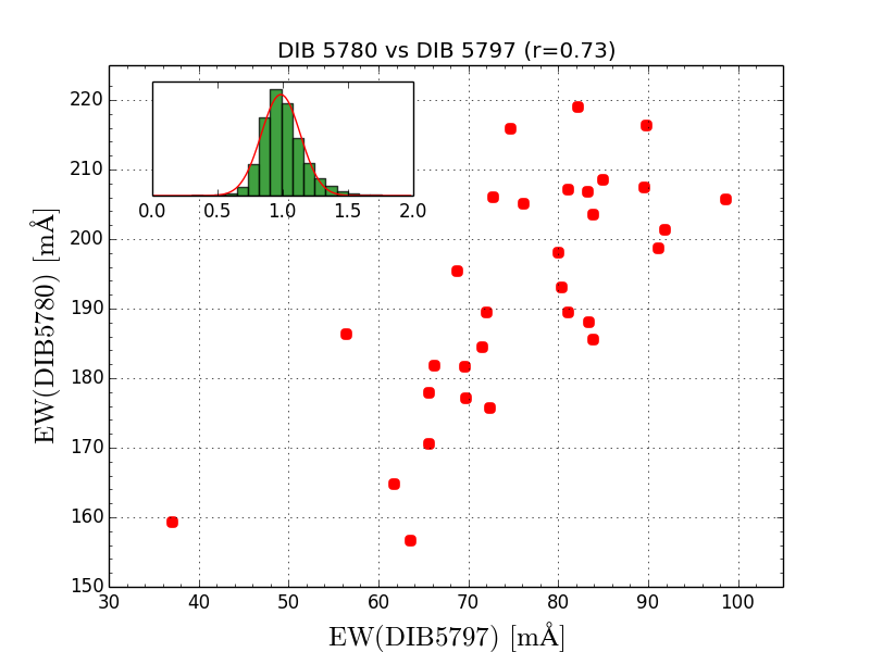
Figure 11: Equivalent widths of DIB 5780, vs 5797. The inset in the upper-left shows the distribution of the derived slope based on 5,000 bootstrap samples. The Gaussian fit in red corresponds to 0.99 $\pm$ 0.15

Fig. 17 shows the derived equivalent widths in the context of the universal DIB correlations detected in many sightlines. While we are in excellent agreement with the general trend, we observe such correlations in our comparably small field of view as well. The common correlation of DIB5780 to DIB 5797 is plotted in Fig. 11 for 31 bins within our FOV. The correlation coefficient is $r=0.73$ and a linear fit to 5,000 bootstrap-realizations of the sample show a slope of $0.99\pm 0.15$. The tight correlation of DIB 5780 and DIB 5797 appears to be universal on all observed scales. Former measurements of the DIB 5780 to DIB 5797 relation as summarized in Friedman et al. (2011) yield a very consistent ratio of $\approx$ 2.3:1 with an offset of about 30 mÅ. While the measurement on the combined data reproduces that relationship exactly, the observed trend of our 31 spatial measurements within the physical absorber shows a slope of almost exactly one. Figure 12 shows the two data sets and their best linear fit. For this single pointing it is hard to judge whether this provides a deeper insight into the nature of the corresponding chemically related carriers. That is one result of this pilot study that we hope to explore further in a much larger investigation based on up to 25 globular clusters. It will show whether the local trend in fact deviates from the universal mixing. Interpreting the DIB ratio 5780/5797 as proxy for gas density (see Sect. 4.3) it can be derived that the regions of higher optical depth also trace the denser gas regions. This can also be seen in Fig. 9 and Fig. 10.

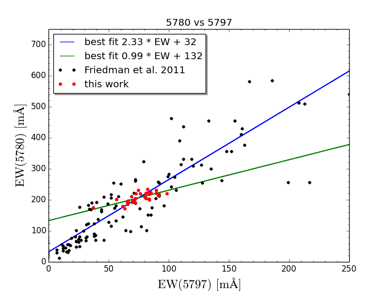
Figure 12: Equivalent widths of DIB 5780, vs 5797 from Friedman et al. (2011) (black) and this work (red) along with a linear best fit. While the average ratio of DIB 5780 to 5797 matches the universal trend perfectly, the observed relation within the absorber differs (see Fig. 11).

The filament structure of Fig. 7 is not seen in $\rm K\,{\scriptstyle I}$ which in principle should be more sensitive to structure. The bottom map in Fig. 8 as well as that in Fig. 9 demonstrate that the doublet ratios, which indicate optical depth, trace each other rather well. The total abundances measured as equivalent widths, however, do not show the same structures. Reliable measurements of the column densities are not feasible at the given spectral resolution. Graham et al. (2015) observe a behavior of interstellar $\rm K\,{\scriptstyle I}$ vs $\rm Na\,{\scriptstyle I}$ that could be explained by it being more sensitive to UV radiation than $\rm Na\,{\scriptstyle I}$ . Smith et al. (2013) describe in their study of small-scale structure in the interstellar medium that $\rm Na\,{\scriptstyle I}$ and $\rm Ca\,{\scriptstyle II}$ were present throughout the cloud, but $\rm Ca\,{\scriptstyle I}$ was only present in the denser regions with $\rm K\,{\scriptstyle I}$ being intermediate between $\rm Na\,{\scriptstyle I}$ and $\rm Ca\,{\scriptstyle I}$ . Thus, one possible explanation for our observations is that the region of stronger $\rm K\,{\scriptstyle I}$ absorption traces an area of a certain density and shielding from UV photons, while the broader area is less favorable for $\rm K\,{\scriptstyle I}$ than $\rm Na\,{\scriptstyle I}$ . The structures of $\rm Na\,{\scriptstyle I}$ and $\rm K\,{\scriptstyle I}$ will be an important part for future analyses. At present we cannot explain this behavior satisfactorily. The coming follow up study of numerous GC observations of MUSE will unfold if such a local trend can be observed commonly.

5.5 Anti-correlation between DIB 6283 and other DIBs

Unexpectedly, all mentioned DIBs anti-correlate with DIB 6283. Other studies observe a universal correlation between DIB 6283 and DIB 5780 that is similar in strength to that of DIB 5797 to DIB 5780 (e.g., Friedman et al. 2011). This section will discuss the meaning and credibility of such an anti-correlation.

The maps and ratios for $\rm K\,{\scriptstyle I}$ and $\rm Na\,{\scriptstyle I}$ as well as for the other DIBs verify the success of the handling of the telluric absorption lines. The templates used for the telluric absorption lines, are based on the best match to a model grid with only the abundance of H₂O  and O₂/O₃  as free parameters.

While telluric O₂  overlaps with DIB 6283 and the $\rm K\,{\scriptstyle I}$ 7664, 7699 features, the fitted O₂  abundance is not able to induce an anti-correlation between DIB 6283 and $\rm K\,{\scriptstyle I}$ . Furthermore, the correction for O₂  works remarkably well, as demonstrated by the tight correlation in Fig. 4, which gives us confidence in the result for DIB 6283 as well. Figure 14 shows the strengths of O₂  in the best fit sky model. The inner pointings that show stronger O₂ absorption, belong to five consecutive exposures during one night as illustrated on the bottom panel of Fig. 14. This impacts some of the central fields of the map, which also showed the weakest DIB 6283 strengths.

Figure 13 shows the difference of the two extreme cases in the data set: two exposures for which the sky model contained the strongest and the weakest O₂  while other telluric model parameters remained similar. The modeled absorption for O₂  varies within a few percent only and affects DIB5780, 5797 and DIB 6283 in an almost identical manner, whereas the effect for $\rm K\,{\scriptstyle I}$ 7664 is about twice as strong and less than half as strong for $\rm K\,{\scriptstyle I}$ 7699. The strength of the telluric feature blending with DIB 6283 is of the same order of magnitude but a little weaker than the DIB itself for this particular target with considerably high extinction. A variation of a few percent here as indicated in Fig. 13 alone can not explain the measured range of DIB 6283 from 380 mÅ  to 470 mÅ. For comparison: the telluric features in the region of the $\rm K\,{\scriptstyle I}$   lines are about 30 times stronger than the $\rm K\,{\scriptstyle I}$   features themselves which show no unusual behavior (see section 3.3).

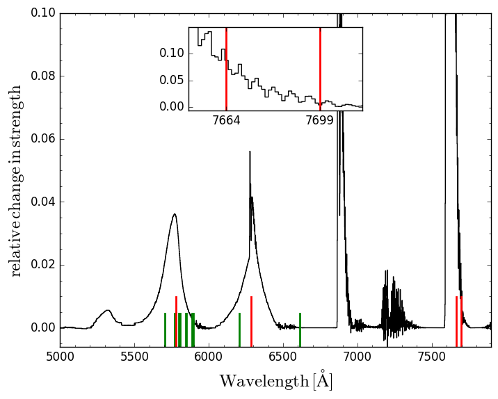
Figure 13: Maximum difference in modeled O₂  absorption relative to the total mean of all exposures. Positions of observed DIBs indicated in green. The red lines mark DIB 5780, DIB 6283 and the $\rm K\,{\scriptstyle I}$   doublet at 7664, 7699Å, which is also shown in the inset at the top.

At the MUSE resolution, DIB 5705 is strongly blended with a stellar line as well but its equivalent width shows no correlation with the background sources at all (see Fig. 15), despite being on the order of the stellar feature and we therefore have confidence that our measurement is reliable.

The stellar $\rm Na\,{\scriptstyle I\,D}$ lines are excluded from the stellar fit and simply scaled with the model. The equivalent width of DIB 6283 in the composite spectrum matches the expectations exactly which rules out notable systematic offsets or misfits. It is possible that the universal behavior of DIB 6283 is just governed by the amount of interstellar material and mixing of chemical abundances in general, whereas we are tracing the DIBs relative to others within a physical environment that shows inhomogeneities in density, temperature and shielding of UV photons on small scales. DIB 6283 could favor regions of ionized gas (see also Ensor et al. 2017). Milisavljevic et al. (2014) noted diametrically opposed behavior of DIB 5780 and DIB 6283 over time in the spectra toward a fading super-nova. In the Milky Way, stronger UV radiation fields tend to lead to weakened DIB 5797 but enhanced DIB 5780 and DIB 6283 (e.g. Ehrenfreund & Jenniskens 1995).

Assuming stronger UV radiation from the bottom-right in the FOV could explain why we observe higher equivalent widths for DIB 6283 toward that direction where it gets ionized first. The same applies for the DIB 5780/5797 ratio, which is strongest toward that direction (see Fig. 7, bottom and Fig. 8, left center).

The amplitude of the variation in the field of view is $\approx 80$ mÅ  for DIB 6283. Inaccurate modeling of stellar lines in this particular spectral region is still a possible source for systematics though the distribution of measured equivalent width strengths is not directly linked to any quantity of the cluster itself. Future analyses will help to confirm or refute this result.

The map of DIB 5705 in Fig. 15 also shows no clear correlation with the other species. While it is affected by a stellar line at 5701.2 Å  the spatial equivalent width distribution does not follow the structure of the globular cluster. Instead it shows a distinct region with an equivalent width that is about 50% higher than for the rest of the field of view.

6 Conclusions

Measuring equivalent widths in $\sim$ 10,000 lines of sight only became feasible with an automatic approach to extracting and modeling stellar spectra as presented in Paper I. Our equivalent width measurements of DIBs in the composite spectrum of thousands of stars reach a very high accuracy down to few m$\AA$. The measured universal ratios are in perfect agreement with results based on high-resolution spectrographs. We evidently resolve small structures in the order of milliparsec and can confirm the correlation of numerous DIBs on small scales within a physically connected region. We demonstrate the feasibility of this approach and outline the main challenges involved.

• The $\rm Na\,{\scriptstyle I}$   doublet shows some filament-like structure in the FOV of $300^{\prime}\times 300^{\prime}$ on the sky against NGC 6397 .

• We mapped a clumpy structure of $\rm K\,{\scriptstyle I}$ with a projected size of $\approx 4,000$ AU assuming a distance of 100 pc.

• We were able to trace optical depth changes of the absorber across the field of view via line ratios of the doublets of $\rm Na\,{\scriptstyle I}$   and $\rm K\,{\scriptstyle I}$   (and more indirectly from the DIB 5780/5797 ratio).

• The projected spatial distribution of DIB 5705 observed in the mapped equivalent widths in Fig. 15 stands out as being particularly inhomogeneous. While the overall equivalent width of DIB 5705 is rather low with $\approx 40$ mÅ  a value above 60 mÅ  at the bottom right extends across several independent bins. This could indicate an independent carrier of DIB 5705. It remains an exciting species for our analysis of further GC sight lines.

• A puzzling finding is the anti-correlation of DIB 6283 with several DIBs. It is the strongest against DIB 5797 and $\rm K\,{\scriptstyle I}$ . We have rejected several systematic errors in the sky modeling, correlations with the environmental conditions of the observations and reduction issues as possible cause of this effect. The findings support the possibility of the carrier of DIB 6283 favoring regions of ionized gas. A future study based on more targets will have to evaluate whether the behavior of DIB 6283 is commonly observed and whether the detected ratios of DIB 5780/5797 which deviate from the universal trend is typical on local scales.

We currently target 25 GCs with VLT/MUSE. Most of them will be observed in several epochs which will give another boost in S/N as well as constraints on temporal variability and tangential motions. We open a new window on studying DIBs spatially resolved at very small scales. This initial pilot study demonstrates the feasibility of the instrument to trace ISM structures despite its comparably low spectral resolution.

Appendix A

A.1 Modeling of absorption features

As briefly described in Section 4.1, all absorption features were modeled with the evolutionary algorithm described in Quast et al. (2005) and applied for molecular species in Wendt & Molaro (2012); Wendt (2014). The $\rm K\,{\scriptstyle I}$ and $\rm Na\,{\scriptstyle I}$   features were fitted as Voigt profiles together with a low order polynomial for the local continuum and taking the appropriate instrument resolution into account. For the $\rm K\,{\scriptstyle I}$ doublet and $\rm Na\,{\scriptstyle I\,D}$ doublet both transitions of each doublet shared the same broadening parameter. In the high resolution UVES spectrum multiple velocity components were resolved for the $\rm Na\,{\scriptstyle I\,D}$ doublet and fitted simultaneously at a tied velocity offset. The wavelength range of $\rm K\,{\scriptstyle I}$ was not covered in the available UVES the data.

The broad DIB features have no complex line profile at the resolution of these data. Many are known to show asymmetric shapes, even though that is barely resolved by MUSE. This was taken into account by fitting regions of DIBs with usually two Gaussians to each observed DIB feature simultaneously. The equivalent widths were derived by integrating over the modeled Gaussians per DIB individually to account for possible overlap regions.

A.2 Complementary plots and maps

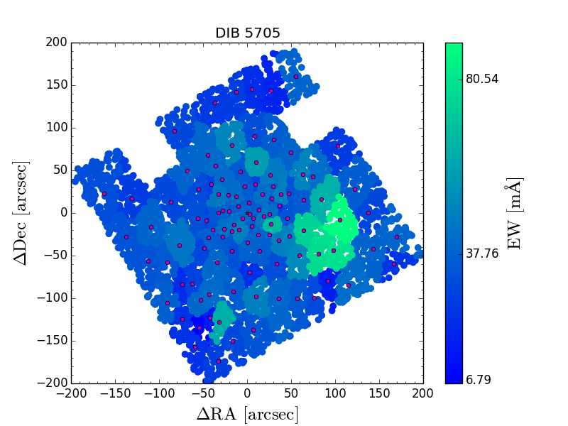
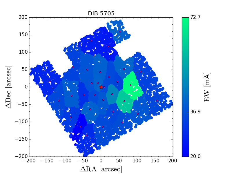
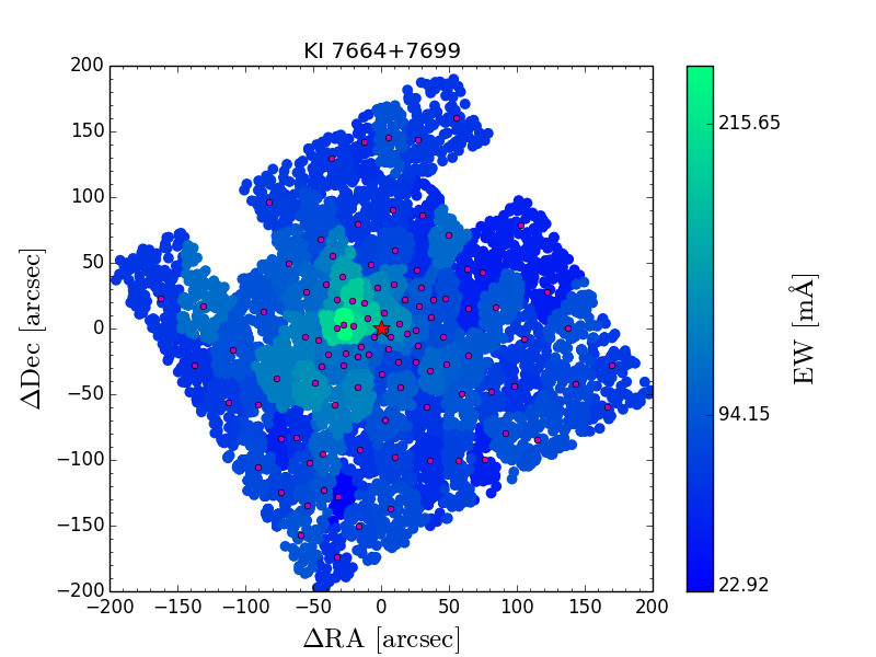
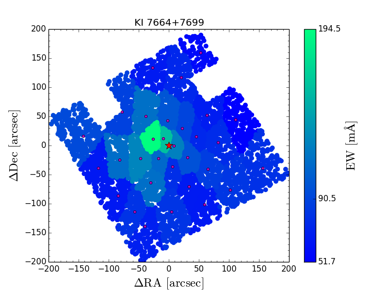
Figure 15: top: Equivalent width maps for DIB 5705. On the left with 107 bins, on the right with 31 bins. bottom:for the $\rm K\,{\scriptstyle I}$ doublet. On the left with 107 bins, on the right with 31 bins. The magenta circles mark the individual Voronoi bins. The red star denotes the cluster’s center. The uncertainty is in the order of 14 mÅ  for the high resolution map and 8 mÅ  for the 31 bins on average.

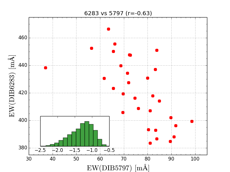
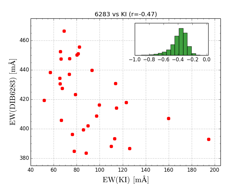
Figure 16: Equivalent widths of DIB 6283 vs DIB 5797 and $\rm K\,{\scriptstyle I}$ .

References

- Ádámkovics et al. (2005) Ádámkovics, M. and Blake, G. A. and McCall, B. J. 2005, ApJ, 625, 857-863
- Andrews et al. (2001) Andrews, S. M., Meyer, D. M. & Lauroesch, J. T. 2001, ApJ, 552, L73
- Bailey et al. (2015) Bailey, M. and van Loon, J. T. and Sarre, P. J. and Beckman, J. E. 2015 MNRAS, 454, 4013-4026
- Bates et al. (1991) Bates, B., Gilheany, S., Wood, K. D. 1991, MNRAS, 252, 600
- Boissé et al. (2013) Boissé, P. and Federman, S. R. and Pineau des Forêts, G. and Ritchey, A. M. 2013, A&A, 559, 131
- Cami et al. (1997) Cami, J., Sonnentrcuker, P., Ehrenfreund, P. & Foing, B.H. 1997, A&A, 326, 822
- Cappellari & Copin (2003) Cappellari, M. and Copin, Y. 2003 MNRAS, 342, 345-354
- Cohen (1978) Cohen, J. G. 1978, ApJ, 223, 487
- Cordiner et al. (2013) Cordiner, M.A. and Fossey,S. J. and Smith, A. M. and Sarre, P. J. 2013 ApJ, 764, L10
- Cox (2011) Cox, N. L. J. 2011, EAS Publications Series, 46, 349-354
- Crawford et al. (1985) Crawford, M.K., Tielens, A.G.G.M., Allamandola, L.J. 1985, ApJ, 293, L45
- Ehrenfreund & Jenniskens (1995) Ehrenfreund, P. and Jenniskens, P. 1995, Astrophysics and Space Science Library, 202, 105
- Ehrenfreund et al. (2002) Ehrenfreund, P. et al. 2002, ApJ, 576, L117
- Ellison et al. (2008) Ellison, S. L. and York, B. A. and Murphy, et al. 2008, MNRAS, 383, L30
- Ensor et al. (2017) Ensor, T. and Cami, J. and Bhatt, N. H. and Soddu, A. 2017, ApJ, 836, 162
- Fabricius et al. (2016) Fabricius, C. and Bastian, U. and Portell et al. 2016, A&A, 595, A3
- Frail et al. (1994) Frail, D. A. and Weisberg, J. M. and Cordes, J. M. and Mathers 1994, ApJ, 436, 144-151
- Friedman et al. (2011) Friedman, S. D. and York, D. G. and McCall et al. 2011 ApJ, 727, 33
- Frisch et al. (2011) Frisch, P. C. and Redfield, S. and Slavin, J. D. 2011 ARA&A, 49, 237-279
- Gaia Collaboration (2016) Brown, A. G. A. and Vallenari, A. and Prusti, T. et al. 2016, A&A, 595, A2
- Graham et al. (2015) Graham, M. L. and Valenti, S. and Fulton, B. J. et al. 2015, ApJ, 801, 136
- Harris (2010) Harris, W. E 2010 astro-ph.GA, 1012.3224
- Hartmann (1904) Hartmann, J. 1904,ApJ, 19
- Heger (1922) Heger, M.L., 1922, Lick Obs. Bull., 10, 146
- Herbig (1995) Herbig, G.H. 1995, ARA&A, 33, 19
- Hubrig et al. (2009) Hubrig, S. and Castelli, F. and de Silva et al. 2009 A&A, 499, 865-878
- Husser et al. (2013) Husser, T.-O., Wende-von Berg, S., Dreizler, S., et al. 2013, A&A, 553
- Husser & Ulbrich (2014) Husser, T.-O. & Ulbrich, K. 2014, Astronomical Society of India Conference Series, 11
- Husser et al. (2016) Husser, T.-O. and Kamann, S. and Dreizler, S. and Wendt et al. 2016 A&A, 588, A148 (Paper I)
- Kalberla et al. (2010) Kalberla, P. M. W. and McClure-Griffiths, N. M. and Pisano et al. 2010, A&A, 521, A17
- Kalberla et al. (2015) Kalberla, P. M. W. and Burton, W. B. and Hartmann, D. and Arnal, E. M. and Bajaja, E. and Morras, R. and Pöppel, W. G. L. 2015, A&A, 440
- Kamann et al. (2013) Kamann, S. and Wisotzki, L. and Roth, M. M. 2013, A&A, 549, A71
- Kamann et al. (2016) Kamann, S. and Husser, T.-O. and Brinchmann et al. 2016 A&A, 588, A149 (Paper II)
- Lallement et al. (2014) Lallement, R. and Vergely, J.-L. and Valette et al. 2014 A&A, 561, A91
- Malamut et al. (2014) Malamut, C. and Redfield, S. and Linsky, J. L. and Wood, B. E. and Ayres, T. R. 2014, ApJ, 787, 75
- McClure-Griffiths et al. (2009) McClure-Griffiths, N.M., et al. 2009, ApJS, 181, 398
- Meyer & Blades (1996) Meyer, D. M. & Blades, J. C. 1996 ApJ, 464, L179
- Meyer & Lauroesch (1999) Meyer, D. M. & Lauroesch, J. T. 1999, ApJ, 520, L103
- Milisavljevic et al. (2014) Milisavljevic, D. and Margutti, R. and Crabtree et al. 2014 ApJ, 782, L5
- Monreal-Ibero et al. (2015) Monreal-Ibero, A. and Lallement, R. and Puspitarini, L. and Bonifacio, P. and Monaco, L. 2015 Mem. Soc. Astron. Italiana, 86, 527
- Monreal-Ibero et al. (2015b) Monreal-Ibero, A. and Weilbacher, P. M. and Wendt et al. 2015,A&A, 576, L3
- Monreal-Ibero & Lallement (2017) Monreal-Ibero, A. and Lallement, R. 2017, A&A, 599, A74
- Nasoudi-Shoar et al. (2010) Nasoudi-Shoar, S. and Richter, P. and de Boer, K. S. and Wakker, B. P. 2010, A&A, 520, A26
- Puspitarini et al. (2013) Puspitarini, L. and Lallement, R. and Chen, H.-C. 2013, A&A, 555, A25
- Puspitarini et al. (2014) Puspitarini, L. and Lallement, R. and Vergely, J.-L. and Snowden, S. L. 2014 A&A, 566, A13
- Quast et al. (2005) Quast, R. and Baade, R. and Reimers, D. 2005, A&A, 431, 1167-1175
- Redfield & Linsky (2008) Redfield, S. & Linsky, J. L. 2008, ApJ, 673
- Sarre (2006) Sarre, P.J. 2006, Journal of Molecular Spectroscopy, 238, 1
- Savage & Sembach (1996) Savage, B. D. and Sembach, K. R. 1996, ApJ, 470, 893
- Schlegel et al. (1998) Schlegel, D. J. and Finkbeiner, D. P. and Davis, M. 1998, ApJ, 500, 525-553
- Sfeir et al. (1999) Sfeir, D. M. and Lallement, R. and Crifo, F. and Welsh, B. Y. 1999 A&A, 346, 785-797
- Smith et al. (2013) Smith, K. T. and Fossey, S. J. and Cordiner et al. 2013, MNRAS, 429, 939-953
- Stanimirović et al. (2010) Stanimirović, S. and Weisberg, J. M. and Pei et al. 2010, ApJ, 720, 415-434
- Thorburn et al. (2003) Thorburn, J. A. and Hobbs, L. M. and McCall, B. J. et al. 2003 ApJ, 584, 339-356
- van Loon et al. (2009) van Loon, J. T. and Smith, K. T. and McDonald, I. et al. 2009 MNRAS, 399, 195-208
- van Loon et al. (2013) van Loon, J.Th., et al. 2013, A&A, 550, 108
- van Loon et al. (2015) van Loon, J. T. and Farhang, A. and Javadi, A. et al. 2015 Mem. Soc. Astron. Italiana, 86, 534
- Vos et al. (2011) Vos, D. A. I. and Cox, N. L. J. and Kaper, L. and Spaans, M. and Ehrenfreund, P. 2011, A&A, 533, A129
- Walker (1963) Walker, G. A. H., MNRAS, 125, 141
- Watson & Meyer (1996) Watson, J. K. and Meyer, D. M. 1996, ApJ, 473, L127
- Weilbacher et al. (2012) Weilbacher, P. M. and Streicher, O. and Urrutia, T. et al. 2012 SPIE Proceedings, 8451, 84510B
- Welsh et al. (2010) Welsh, B. Y. and Lallement, R. and Vergely, J.-L. and Raimond, S. 2010 A&A, 510, A54
- Welty & Hobbs (2001) Welty, D. E. and Hobbs, L. M. 2001 ApJS, 133, 345-393
- Welty et al. (2006) Welty, D. E. and Federman, S. R. and Gredel, R. and Thorburn, J. A. and Lambert, D. L. 2006 ApJS, 165, 138-172
- Wendt & Molaro (2012) Wendt, M. and Molaro, P. 2012, A&A, 541, A69
- Wendt (2014) Wendt, M. 2014, Astronomische Nachrichten, 335, 106
- Williams (1994) Williams, R. E. 1994, ApJ, 426, 279