Thermal rupture of a free liquid sheet

Abstract

We consider a free liquid sheet, taking into account the dependence of surface tension on temperature, or concentration of some pollutant. The sheet dynamics are described within a long-wavelength description. In the presence of viscosity, local thinning of the sheet is driven by a strong temperature gradient across the pinch region, resembling a shock. As a result, for long times the sheet thins exponentially, leading to breakup. We describe the quasi one-dimensional thickness, velocity, and temperature profiles in the pinch region in terms of similarity solutions, which posses a universal structure. Our analytical description agrees quantitatively with numerical simulations.

1 Introduction

The breakup of liquid sheets plays a crucial role in the generation of industrial sprays Eggers & Villermaux (2008) or natural processes such as sea spray Wu (1981). The industrial production sprays proceeds typically via the formation of sheets Eggers & Villermaux (2008), which break up to form ribbons. Ribbons are susceptible to the Rayleigh-Plateau instability, and quickly break up into drops. In nature, sheets are often formed by bubbles rising to the surface of a pool Boulton-Stone & Blake (1993); Lhuissier & Villermaux (2011). Once broken, the sheet decays into a mist of droplets Lhuissier & Villermaux (2011); Feng et al. (2014), and collapse of the void left by the bubble produces a jet Duchemin et al. (2002).

It is therefore of crucial importance to understand the mechanisms leading to the breakup of sheets. In contrast to jets and liquid threads, there is no obvious linear mechanism for sheet breakup, unless there is strong shear, and the mechanism is that of the Kelvin-Helmholtz instability Tammisola et al. (2011). As a result, authors have invoked the presence of attractive van-der-Waals forces Vrij (1966) to explain spontaneous rupture Thoroddsen et al. (2012). However, the mean sheet thickness near the point of breakup is often found to be several microns, while van-der-Waals forces only have a range of nanometers, and cannot play a significant role except perhaps for the very last stages of breakup.

Instead, it has been suggested Tilley & Bowen (2005); Bowen & Tilley (2013); Lhuissier & Villermaux (2011); Néel & Villermaux (2017) that gradients of temperature could promote breakup, because they produce Marangoni forces Craster & Matar (2009), which lead to flow. This cannot be a linear mechanism, since for reasons of thermodynamic stability Marangoni flow will always act to reduce gradients; molecular diffusion will also alleviate (temperature) gradients. Finally, the extensional flow expected near a potential pinch point will stretch the fluid particles, once more tending to reduce gradients. It is therefore surprising that temperature gradients can promote breakup, and if this is the case, the mechanism must be inherently non-linear.

In the absence of viscosity, it was found numerically that sheets can break up in finite time Matsuuchi (1976); Pugh & Shelley (1998), if there is a sufficiently strong initial flow inside the sheet. This was confirmed analytically by Burton & Taborek (2007), who found a similarity solution leading to finite-time breakup. Their solution is slender, so a long-wavelength approximation can be used, and the final stages of breakup are described by a local mechanism. However it is found numerically Bowen & Tilley (2013) and supported by theoretical arguments Eggers & Fontelos (2015), that an arbitrary small amount of viscosity inhibits this singularity, and the sheet returns ultimately to its original equilibrium thickness. Scaling arguments suggest that the minimum thickness reached is in the order of the viscous length scale $\ell_{\nu}=\nu^{2}\rho/\gamma$ Eggers & Dupont (1994), which even for a low viscosity liquid such as water only reaches about 10 nm.

Bowen & Tilley (2013) have thus asked the question whether in the non-linear regime, temperature gradients could remain effective in driving the sheet toward vanishing thickness. If there is no viscosity, yet temperature (and thus surface tension) gradients are taken into account, the Burton & Taborek (2007) singularity is recovered, and surface tension gradients play a subdominant role. This is consistent with the above argument that a pinching solution will only stretch, and thus alleviate, thermal gradients. However paradoxically, numerical evidence suggests Bowen & Tilley (2013) that if both finite viscosity and surface tension gradients are taken into account, breakup can occur, by a mechanism different from those considered previously. However, Bowen & Tilley (2013) were unable to find a consistent similarity description, and numerical evidence is inconclusive as to whether there is a finite time or infinite time singularity. Let us also mention a recent study Néel & Villermaux (2017) of the initial stages of sheet rupture from both an experimental and an analytical point of view. In particular, the authors provide an explanation for the formation of a sharp temperature jump within the thin pinch-off region, which has been observed by Bowen & Tilley (2013) to persist during the later self-similar evolution of the sheet.

In this paper, we address the late stages of pinch-off in the presence of both finite viscosity and surface tension gradients. For simplicity, here we only consider variations of the temperature. These are the equations for a surfactant in the limit of high solubility Jensen & Grotberg (1993); Matar (2002). In the next section, we describe the equations coming from a long-wavelength assumption: the sheet thickness is much smaller than a typical variation in the lateral direction. This description is one-dimensional, in that gradients in only one direction along the sheet are considered important. We also describe a finite differences numerical code and show some typical solutions leading to rupture, an example of which is shown in Fig. 1. Starting from smooth initial profiles for the sheet thickness $h(x,t)$, velocity $u(x,t)$, and temperature $\theta(x,t)$, the shape of the sheet evolves toward a thin film on the left, connected to a macroscopic droplet right, see Fig. 1 (a). A zoom of the pinch region (Fig. 1 (b)) shows that the sheet thickness goes to zero in a localized fashion near the point where the sheet and the drop meet. In the same region, the velocity has a sharp and increasing maximum (Fig. 1 (c)), while the temperature develops an increasingly sharp jump (Fig. 1 (d)).

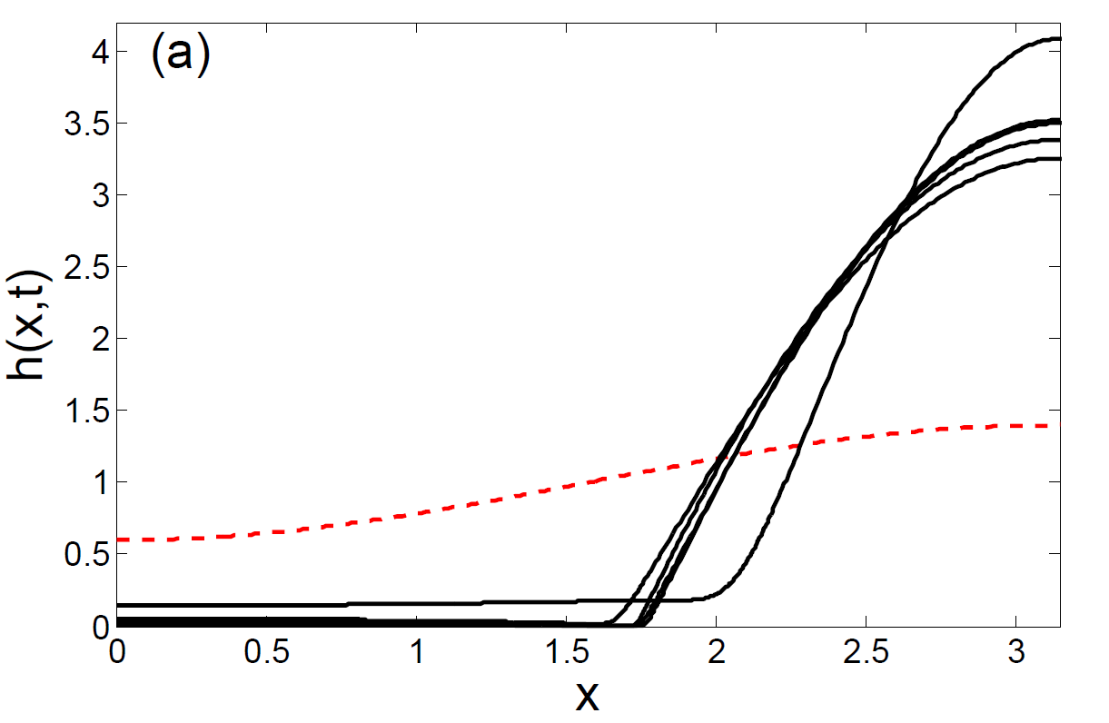
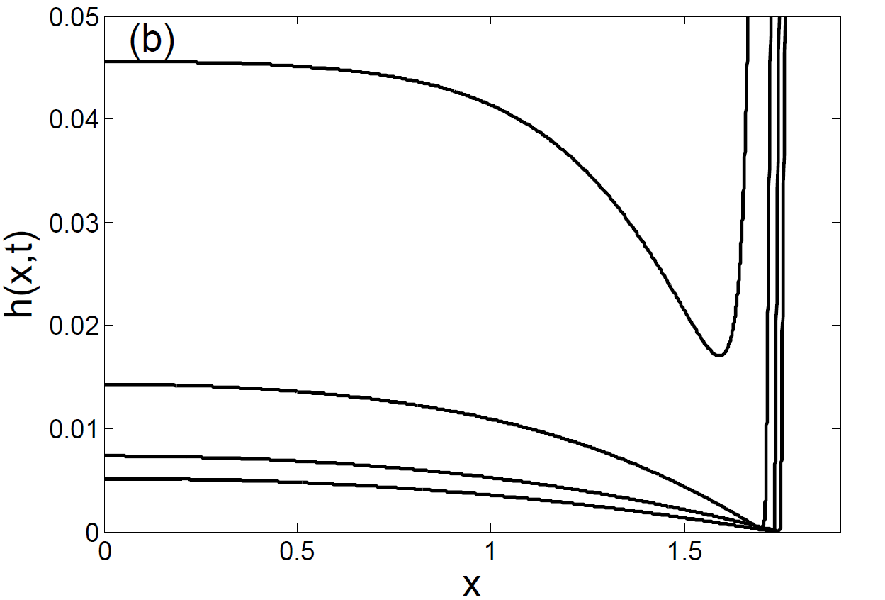
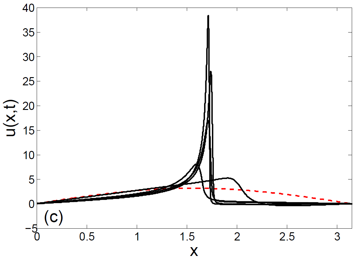
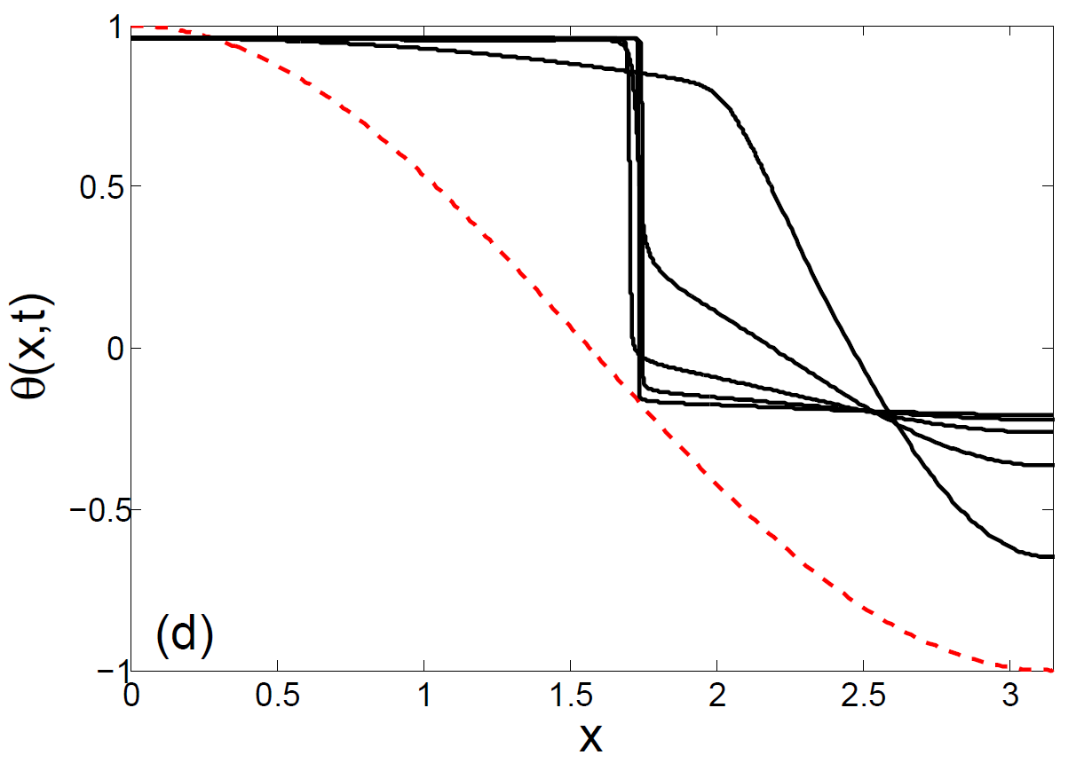
Figure 1: Rupture of a viscous liquid sheet as described by (2), starting from initial conditions $h(x,0)=1-0.4\cos(x)$, $u(x,0)=\pi\sin(x)$, and $\theta(x,0)=\cos(x)$, a particular case of those used in Bowen & Tilley (2013) (red dashed curves), with parameters ${\cal O}={\cal D}=1/4$ and ${\cal M}=10$. Shown are six snapshots, taken at times $t_{0}=0,\,t_{1}=2.247,\,t_{2}=4.032,\,t_{3}=5.138,\,t_{4}=5.987,\,t_{5}=6.800$, of the height profile $h(x,t)$ (a), with a zoom of the pinch region shown in (b). The velocity $v(x,t)$ and temperature $\theta(x,t)$ profiles are shown in (c) and (d), respectively.

In the third section, we construct an analytical solution in which the sheet thickness goes to zero exponentially. The macroscopic outer part consists of an exponentially thinning film, on one side, and a static “bubble” on the other. Over both parts of the outer solution the temperature is approximately constant but different, with a strong gradient between the two regions. The pinch region connecting the two parts is described by two different similarity solutions, which hold in two different regions, with two different sets of scaling exponents. Matching all regions together, we are able to describe pinch-off in terms of a single free parameter, which is the position of the pinch point. All other parameters are found in terms of the initial conditions, or can be absorbed into a shift in time. The results agree very well with numerical simulations of the long-wavelength equations. We show for the first time, both theoretically and numerically (see Fig. 4), that the minimum of the sheet thickness $h(x,t)$ decreases exponentially, at a rate we calculate. In a final section, we discuss our results and give perspectives. The Appendix presents a detailed analysis of the leading order equation arising in the exponentially thinning film region and contains a complete list of its possible solutions.

2 Long-wavelength equations and simulation

We consider the motion of a free liquid sheet, whose plane of symmetry has been fixed in the $z$-plane. We expect that generically the sheet breaks up along a line, so in describing this singularity, we can assume that fields only depend on the coordinate $x$ perpendicular to this line. Thus the shape of the sheet is described uniquely by the half-thickness $h(x,t)$. We assume that the surface tension depends linearly on temperature $\theta$ Craster & Matar (2009) according to

$$\gamma=\gamma_{0}-k\theta,$$ (1)

which is a good approximation away from any critical point Rowlinson & Widom (1982). We will assume that $k>0$ as is the case for most systems, but the opposite sign will simply reverse the flow of heat. The average velocity in the sheet is $u(x,t)$, and the temperature $\theta(x,t)$, which is allowed to diffuse.

Then in the limit of slender sheets Bowen & Tilley (2013), the dimensionless form of the equations is

$$h_{t} =-\left(hu\right)_{x}$$ (2a)

$$u_{t}+uu_{x} =h_{xxx}+4{\cal O}\frac{(hu_{x})_{x}}{h}-{\cal M}\frac{\theta_{x}}{h}$$ (2b)

$$\theta_{t}+u\theta_{x} ={\cal D}(h\theta_{x})_{x},$$ (2c)

where subscripts denote differentiation with respect to the variable. As a length scale, we have chosen $L_{0}=L/\pi$, where $L$ is the width of the computational domain, and $\tau=\sqrt{L_{0}^{3}\rho/\gamma_{0}}$ is the time scale; $\rho$ is the fluid density. As a unit of temperature we take the initial temperature difference $\Delta$ across the system.

Then (2a) describes mass conservation, and (2b) is the momentum balance across the sheet. Inertial forces on the left are balanced by surface tension, viscous stresses, and Marangoni forces on the right, respectively. The size of the kinematic viscosity $\nu$ is measured by the Ohnesorge number ${\cal O}=\nu\sqrt{\rho/(L_{0}\gamma_{0})}$, and the Marangoni number is defined by ${\cal M}=k\Delta\gamma_{0}$. We assume that the variation of the surface tension is small, so we can take it as a constant, except in the Marangoni term. The last equation (2c) describes the diffusion of temperature through the sheet, and ${\cal D}=\gamma\sqrt{\rho/(L_{0}\gamma_{0})}$, where $\kappa$ is the thermal diffusion coefficient; ${\cal P}={\cal O}/{\cal D}$ is known as the Prandtl number.

For simplicity, we consider solutions to (2) in a fixed domain $[0,\pi]$ (after non-dimensionalization), and assume that

$$u=h_{x}=\theta_{x}=0\;\mbox{for}\;x=0,\pi,$$ (3)

i.e. no-flux boundary conditions for the velocity and free boundary conditions for the height and the temperature. This choice of boundary conditions is motivated by the fact that for symmetric initial data, for example those of Fig. 1, they result in solutions which can be extended to periodic solutions of period $2\pi$. The conditions (3) also imply that there is no mass or heat flux out of the system, and thus

$$M=\int_{0}^{\pi}h(x,t)\,dx,\quad Q=\int_{0}^{\pi}\theta(x,t)h(x,t)\,dx$$ (4)

are conserved quantities, set by the initial conditions. We do not expect our choice of boundary conditions to have an effect on the structure of the singularity. The outer film and bubble regions will still be described by the same leading order ODEs, but their solutions may be selected by the particular boundary and initial data. However, with the particular choice of boundary conditions (3) we are able to determine the structure of the singularity largely in terms of the two quantities $M$ and $Q$ alone.

Our main focus will be on pinch-off singularities for which $h\rightarrow 0$ at some point $x_{0}$ in space. To summarize what is known or widely accepted about pinch-off singularities of the system (2), and as stated in the Introduction, for ${\cal O}=0$ finite-time pinch-off can occur for suitable initial conditions. The neighborhood of the pinch point is described by the similarity solution of Burton & Taborek (2007) for any value of ${\cal M}$, and Marangoni forces are subdominant. If on the other hand ${\cal O}$ is finite and ${\cal M}=0$, breakup can never occur Eggers & Fontelos (2015) and instead the sheet will eventually relax to a uniform state $h(x)=M$. The present paper deals with the case that both ${\cal M}$ and ${\cal O}$ are nonzero, for which we find a local pinch solution for which the thickness goes to zero exponentially in time (a typical example being presented in Fig. 1).

To solve the system (2) we extended the finite-difference schemes developed previously for the modeling of finite time rupture under the presence of van der Waals forces by Peschka (2008); Peschka et al. (2010) and of coarsening dynamics of droplets in free liquid films by Kitavtsev & Wagner (2010). We incorporated the temperature equation (2c) along with the Marangoni term -${\cal M}\theta_{x}/h$, coupled with the boundary conditions (3). The resulting fully implicit finite-difference scheme is solved on a general nonuniform mesh in space, with adaptive time step. At every time step the nonlinear system of algebraic equations is solved using Newton’s method. In order to resolve the solution close to the rupture point we applied the algorithm of Peschka (2008) for dynamical grid re-meshing to concentrate points near where the film thickness is the smallest.

3 Self-similar pinch-off solutions

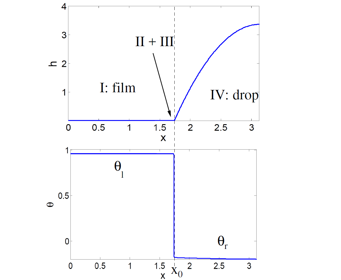
Figure 2: Typical height (top) and temperature (bottom) profiles near pinch-off. On the left, a film (region I) which thins exponentially, on the right a drop in static equilibrium (region IV). These two outer regions are joined together at $x_{0}$, where pinch-off ultimately occurs. The temperature inside the film has a nearly constant value $\theta_{l}$, in the drop a constant value $\theta_{r}$, with a sudden drop in the pinch region. The inner region at the juncture between film and drop has to split into two sub regions (II and III), which have different scalings.

We begin with an overview of the structure of the solution in the asymptotic region we hope to describe, see Fig. 2. The outer solution, observed on a macroscopic scale, is split between a thin film region I on the left, and a drop region IV on the right; the two are joined together at the pinch point $x_{0}$. The film thins exponentially in time, while the drop is in static equilibrium, and has a stationary profile. The temperature is almost constant in the two regions, with a sudden jump near the pinch point. Since the surface tension is lower on the left (higher temperature), this drives a Marangoni flow from the film into the drop, which is responsible for the thinning of the film.

The crucial question is how this strong temperature gradient is maintained, and what stabilizes the sudden jump in temperature. To understand this, one must study the inner region joining the two outer solutions, whose width will turn out to be of the same order as the film thickness, and which is therefore not resolved in Fig. 2. It turns out that in order to achieve a matching between regions I and IV, one must subdivide the inner region into two sub-regions, characterized by similarity solutions with different scalings. The first one, region II, we call the “pinch region”, because the film thickness has its minimum there and it is where pinch-off ultimately occurs. This region is characterized by a balance of inertia, viscosity, and Marangoni forces. However this does not match the drop region, where surface tension alone is important. This necessitates another region III, the “transition region”, where only surface tension and viscosity are important.

The fundamental insight which determines the structure of both similarity solutions is that the flux of liquid across the inner region is set by the flux out of the thin film region, which is set on a macroscopic scale. Thus the flux $j=hu$ across inner regions II and III must be a spatial constant (but does depend on time). We will see that this constraint fixes the scaling exponents, and greatly simplifies the structure of the solution. Curiously, a similar structure was found for Hele-Shaw flow Bertozzi et al. (1994) and viscous films in a capillary tube Lamstaes & Eggers (2017).

We now present all asymptotic regions systematically, and discuss matching between them.

3.1 I: thin film region

The width of this region is of order one, yet the thickness $\tau(t)$ of the film shrinks to zero, so we use the ansatz

$$h(x,t)=\tau(t)h_{f}(x),\quad u(x,t)=u_{f}(x),\quad\theta(x,t)=\theta_{l},$$ (5)

where the temperature is assumed constant, in accordance with our earlier observations. Inserting (5) into the equations of motion, (2a) yields

$$\dot{\tau}h_{f}=-\tau\left(h_{f}u_{f}\right)^{\prime},$$ (6)

and at leading order $\tau^{0}$, (2b) results in

$$u_{f}u_{f}^{\prime}=4{\cal O}\frac{(h_{f}u_{f}^{\prime})^{\prime}}{h_{f}},$$ (7)

where the surface tension term is of order $\tau$, and thus drops out in the limit $\tau\rightarrow 0$. Here and in the remainder of the paper, a dot denotes a derivative with respect to time, a prime with respect to the spatial variable. Note that (7) represents a balance between inertia and viscosity, while surface tension and Marangoni forces drop out. Dividing (6) by $\tau h_{f}u_{f}$ and (7) by $4{\cal O}u_{f}^{\prime}$, the term $h_{f}^{\prime}/h_{f}$ can be eliminated between the two equations, and one obtains an equation for the velocity $u_{f}$ alone:

$$\bar{u}+\frac{\dot{\tau}}{\tau 4{\cal O}\bar{u}}=\frac{\bar{u}^{\prime\prime}}{\bar{u}^{\prime}}-\frac{\bar{u}^{\prime}}{\bar{u}},$$ (8)

where we have rescaled the velocity according to: $u_{f}=4{\cal O}\bar{u}$. In (8) only the second term on the left hand side depends on time. Therefore, necessarily one has $-\dot{\tau}/\tau=4a{\cal O}$, where $a>0$ is a constant, which depends on initial conditions, as we will see. This implies

$$\tau(t)=\tau_{0}\exp\{-4a{\cal O}t\},$$ (9)

$$\bar{u}-\frac{a}{\bar{u}}=\frac{\bar{u}^{\prime\prime}}{\bar{u}^{\prime}}-\frac{\bar{u}^{\prime}}{\bar{u}},$$ (10)

where $\tau_{0}$ is an arbitrary normalization factor, which depends on the choice of origin for the time coordinate.

As shown in the Appendix, (10) can be integrated and posses a one-parameter family of ’blow-up’ solutions of the form:

$$\bar{u}_{A}(x)=A+\tan\left[(x-\bar{x})\sqrt{a-A^{2}}\right]\sqrt{a-A^{2}},\quad\text{for}\ A\in(-\sqrt{a},\sqrt{a}).$$ (11)

The boundary conditions $\bar{u}(0)=\bar{u}^{\prime\prime}(0)=0$, which follow from (3), together with (7), require that $A=\bar{x}=0$, and thus

$$u_{f}=4{\cal O}\sqrt{a}\tan\left(x\sqrt{a}\right).$$ (12)

The flux $j_{f}(x)=h_{f}(x)u_{f}(x)$ is calculated from (6) as

$$\ln j_{f}=\int\frac{4{\cal O}a}{u_{f}}dx,$$ (13)

and then it follows from (12) that

$$j_{f}(x)=j_{0}\sin(\sqrt{a}x),\quad h_{f}(x)=\frac{j_{0}}{4{\cal O}\sqrt{a}}\cos(\sqrt{a}x),$$ (14)

where $j_{0}$ is a positive constant. It is clear from the first equation of (5) that by adjusting $\tau_{0}$, we can make $h_{f}(0)=j_{0}/4{\cal O}\sqrt{a}$ attain any value, which means that $j_{0}$ can be chosen arbitrarily. In the numerical results reported below, we will make the particular choice $j_{0}=4{\cal O}\sqrt{a}$.

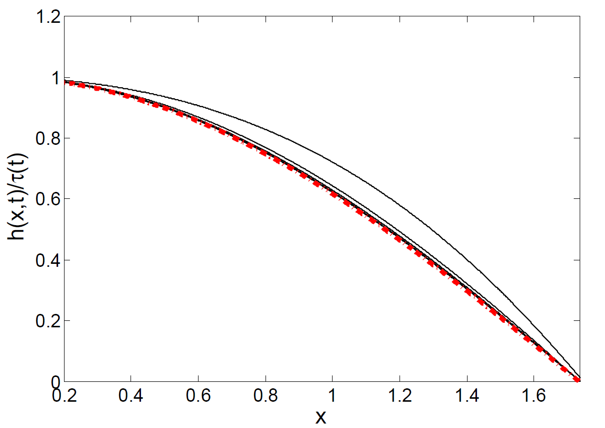
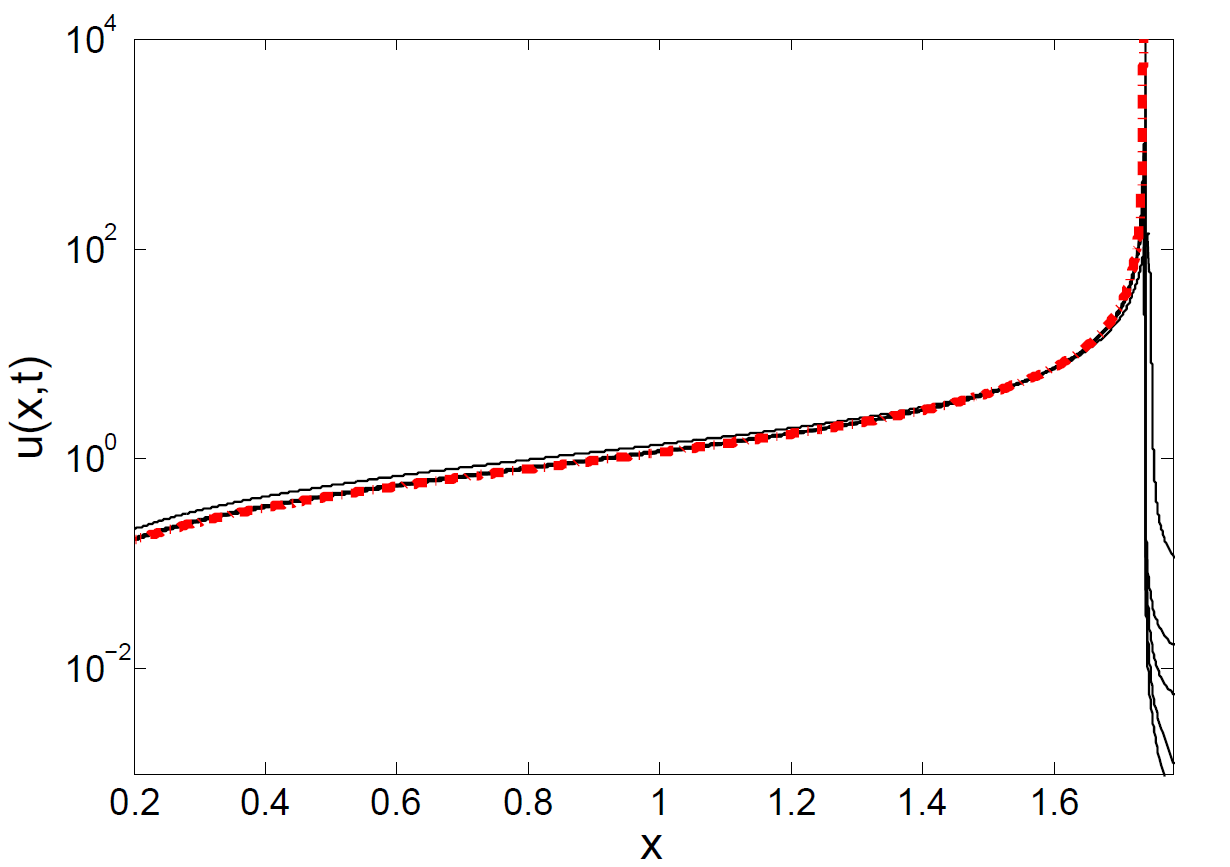
Figure 3: Comparison of a numerical solution of (2) (initial data and parameters as in Fig. 1), with the leading order solutions (14) and (12) (red dash-dotted curves), in the then film region. Five snapshots of the height (left, linear plot) and velocity (right, log-linear plot) solutions to (2) are shown at times $t_{1}=2.247,\,t_{2}=4.032,\,t_{3}=5.138,\,t_{4}=5.987,\,t_{5}=6.800$. The thinning rate $a=0.819$ was calculated from the numerical solution using (10). The pinch point was found to be $x_{0}\approx 1.7355$, in very good agreement with (15).

The pinch point $x_{0}$ is determined by where $h_{f}$ goes to zero, which is at

$$x_{0}=\pi/(2\sqrt{a});$$ (15)

the interval $0\leq x\leq x_{0}$ will be referred to as the “thin film region”. At $x_{0}$, the flux is $j_{f}(x_{0})=j_{0}$, which means that according to (5) the mass flux through the pinch point and into the drop is $\tau j_{0}$. In the neighborhood of $x_{0}$, the outer (film) profiles are

$$h\approx-\frac{j_{0}\tau(x-x_{0})}{4{\cal O}},\quad u\approx-\frac{4{\cal O}}{x-x_{0}}.$$ (16)

In Fig. 3 we present the leading order film solutions (12) and (14) in the thin film region (red dash-dotted curves), superimposed with full numerical solutions, rescaled according to (5). Even for times of order one, very convincing convergence toward the asymptotic solutions is found.

3.2 IV: drop region

The total mass in the film region is of order $\tau$, which means that any change in the volume of the drop region is a subdominant correction. To leading order, the drop volume is constant and the drop thus converges toward a static shape, with no flow, and temperature is constant: $h(x,t)=h_{d}(x)$ and $\theta(x,t)=\theta_{r}$, while $u(x,t)=0$. The leading order solution to (2b) in this region must satisfy $h_{d}^{\prime\prime\prime}=0$, and thus

$$h_{d}(x)=C_{0}\left[(\pi-x_{0})^{2}-(x-\pi)^{2}\right],$$ (17)

where $x_{0}$ is the pinch point as in (15). The constants $C_{0}$ and $\theta_{r}$ are determined uniquely by conservation of mass and heat (4), which yields

$$\int_{x_{0}}^{\pi}h_{d}(x)\,dx=M,\quad\int_{x_{0}}^{\pi}h_{d}(x)\theta_{r}\,dx=Q.$$

From this the constants can be computed as

$$C_{0}=\frac{3M}{2(\pi-x_{0})^{3}},\quad\theta_{r}=\frac{Q}{M}.$$ (18)

In particular, we have the following expression for the macroscopic contact angle of the drop:

$$h_{d}^{\prime}(x_{0})=\frac{3M}{2(\pi-x_{0})^{2}}\equiv s,$$ (19)

which will be used later to match to the pinch region.

3.3 II: pinch region

Since this solution lives on an exponentially small scale set by the film thickness $\tau$, we try the similarity solution

$$h(x,t)=\tau^{\alpha_{1}}H\left(\xi\right),\quad u(x,t)=\tau^{\alpha_{2}}U\left(\xi\right),\quad\theta(x,t)=\tau^{\alpha_{3}}\Theta\left(\xi\right),\quad\xi=\frac{x-x_{0}}{\tau^{\beta}}.$$ (20)

Since the flux through the pinch region is $\tau j_{0}=hu$, we must have $\alpha_{1}+\alpha_{2}=1$. We also expect (20) to match to the linear $h$-profile (16), which implies that $\alpha_{1}-\beta=1$. Since the temperature changes over scale of order unity, we have $\alpha_{3}=0$. Finally, Marangoni forces drive the pinch-off and thus must come in at leading order near the pinch point. We expect them to be balanced by viscous forces, which already come in the thin film region, and thus should also be important on even smaller scales. Then from a balance of the last two terms of (2b) we obtain $\alpha_{2}-2\beta=-\beta-\alpha_{1}$, and combining all of the above yields $\beta=1$, $\alpha_{1}=2$, and $\alpha_{2}=-1$. Then the leading force balance in (2b) is at $O(\tau^{3})$, and inertial, surface tension, and Marangoni forces come in at leading order.

Thus in the pinch region the similarity solution takes the form

$$h(x,t)=\tau^{2}H_{p}\left(\xi\right),\quad u(x,t)=\tau^{-1}U_{p}\left(\xi\right),\quad\theta(x,t)=\Theta_{p}\left(\xi\right),\quad\xi=\frac{x-x_{0}}{\tau},$$ (21)

and the similarity equations are

$$j_{0} =H_{p}U_{p}$$ (22a)

$$U_{p}U_{p}^{\prime} =4{\cal O}\frac{(H_{p}U_{p}^{\prime})^{\prime}}{H_{p}}-{\cal M}\frac{\Theta_{p}^{\prime}}{H_{p}}$$ (22b)

$$U_{p}\Theta_{p}^{\prime} ={\cal D}\left(\frac{H_{p}\Theta_{p}^{\prime}}{H_{p}}\right)^{\prime}.$$ (22c)

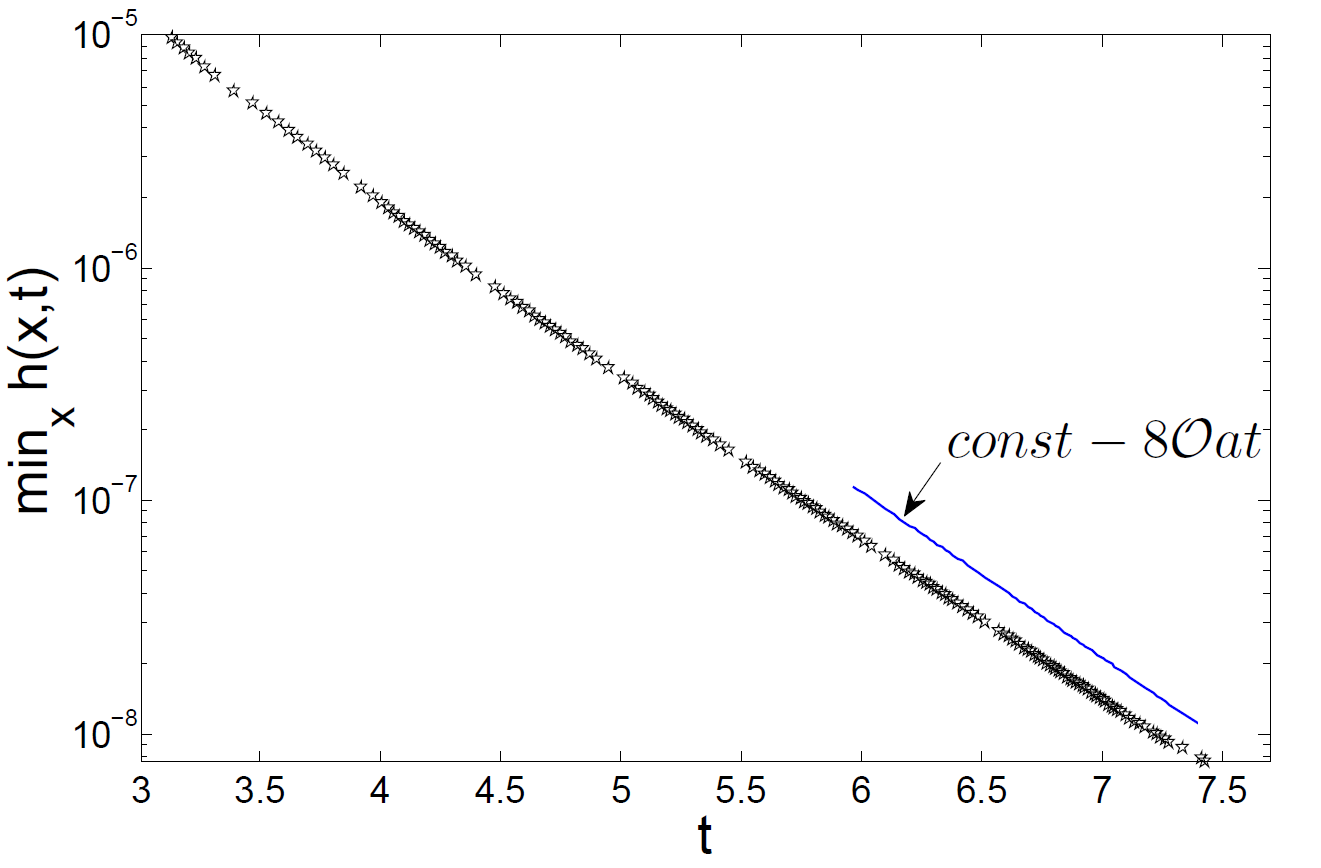
Figure 4: Log-linear plot of the minimum height as function of time (black symbols) for the solution to (2), with parameters and initial data as in Fig. 1 and Fig. 3. The thinning rate $a=0.819$ was calculated from the numerical solution using (10). The blue solid line is the theoretical prediction (23).

In particular, using (9) the minimum sheet thickness decays exponentially:

$${\rm min}_{x}h(x,t)\propto\tau^{2}\propto\exp\{-8a{\cal O}t\},$$ (23)

which is confirmed numerically in Fig. 4.

The flux condition (22a) can be used to eliminate $H_{p}$, and we obtain the two equations

$$U_{p}^{\prime}=4{\cal O}\left(U_{p}^{\prime}/U_{p}\right)^{\prime}-{\cal M}\Theta_{p}^{\prime}/j_{0},\quad\Theta_{p}^{\prime}={\cal D}\left(\Theta_{p}^{\prime}/U_{p}\right)^{\prime}.$$ (24)

Integrating the first equation in (24) one expresses the temperature profile dependence on $U_{p}$ explicitly as

$$\Theta_{p}=\frac{j_{0}}{\cal M}\left(4{\cal O}\frac{U_{p}^{\prime}}{U_{p}}-U_{p}\right)+\theta_{l},$$ (25)

where we have used the boundary conditions on the similarity profiles, as $\xi\rightarrow-\infty$:

$$H_{p}\approx-\frac{j_{0}\xi}{4{\cal O}},\quad U_{p}\approx-\frac{4{\cal O}}{\xi},\quad\Theta_{p}\approx\theta_{l},$$ (26)

which follow from comparison to (16).

Next, substitution of (25) into the second (temperature) equation of (24) gives the following ODE for the profile $U_{p}$:

$$4{\cal D}{\cal O}\left(U_{p}^{\prime\prime}-U_{p}^{\prime 2}/U_{p}\right)-(4{\cal O}+{\cal D})U_{p}^{\prime}U_{p}+U_{p}^{3}+C_{2}U_{p}^{2}=0,$$ (27)

with $C_{2}$ being a constant of integration. Evaluating the left-hand side of (27) for $\xi\rightarrow-\infty$, once more using (26), one concludes that $C_{2}=0$.

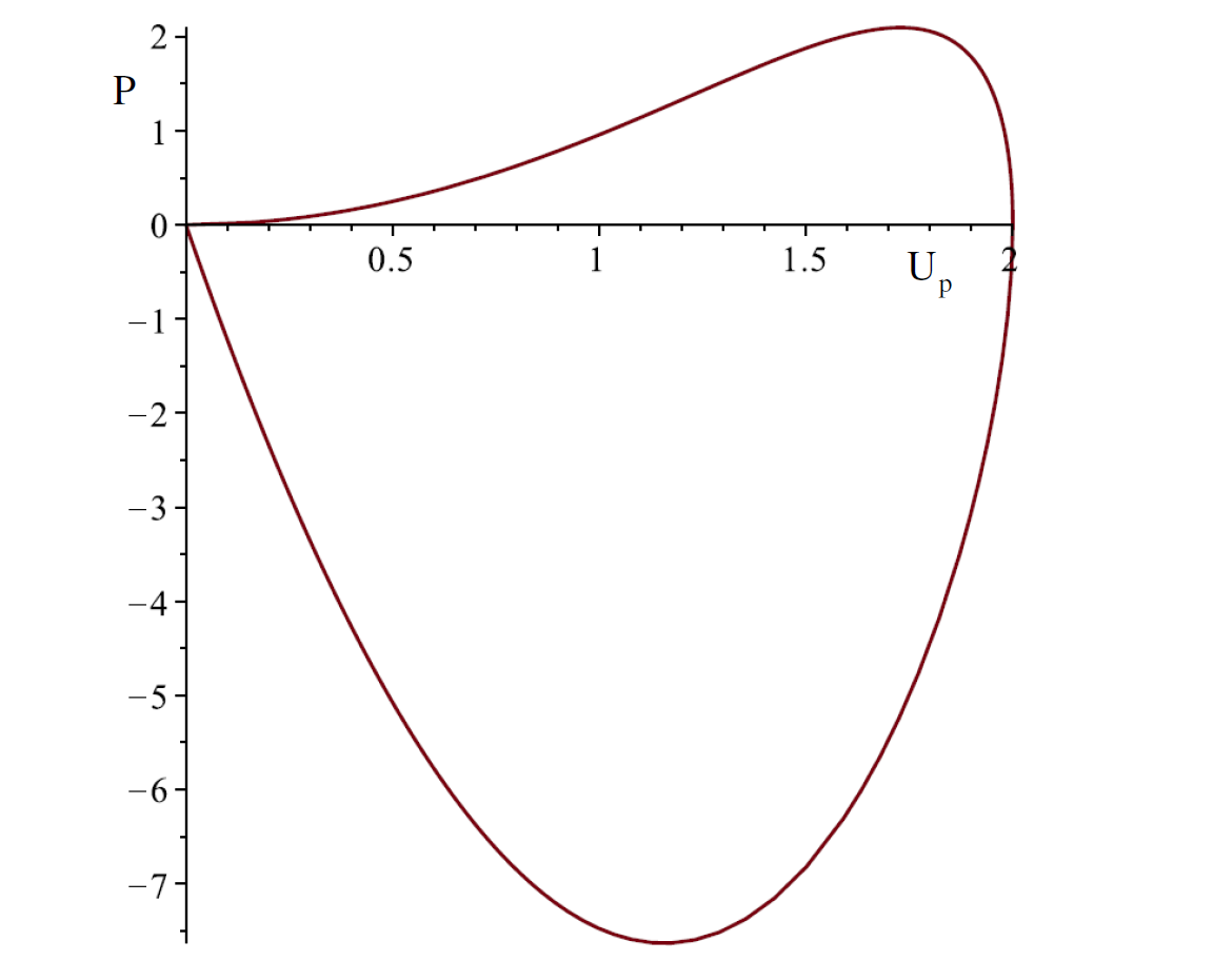
Figure 5: The homoclinic orbit defined by (29)-(33), with $C_{+}=2\cdot 4^{4/3}$ and ${\cal P}=1$.

The second order equation (27) can be turned into a first-order equation putting $U_{p}^{\prime}(\xi)=P(U_{p})$, so that $U_{p}^{\prime\prime}=P^{\prime}P$, and

$$\frac{dP}{dU_{p}}=\frac{P}{U_{p}}+\left({\cal D}^{-1}+(4{\cal O})^{-1}\right)U_{p}-\frac{U_{p}^{3}}{4{\cal D}{\cal O}P}.$$ (28)

The observation that (28) is invariant under $U_{p}\rightarrow C_{+}U_{p}$ and $P\rightarrow C_{+}^{2}P$ suggest the substitution

$$P=\frac{wU_{p}^{2}}{4\sqrt{{\cal D}{\cal O}}},$$ (29)

which reduces (28) to the separable ODE

$$\frac{dU_{p}}{U_{p}}=\frac{dw}{4\sqrt{\cal P}+\sqrt{\cal P}^{-1}-4/w-w}.$$ (30)

From (26) it follows that $w$ must satisfy the boundary condition $w\approx\sqrt{\cal P}^{-1}$ for $U_{p}\rightarrow 0$. Hence for each ${\cal P}>0$ bounded solutions of (30) have the form:

$$U_{p}(w)=\left\{\begin{array}[]{ll}C_{+}\left(\sqrt{\cal P}^{-1}-w\right)^{\frac{1}{4{\cal P}-1}}/\left(4\sqrt{\cal P}-w\right)^{\frac{4{\cal P}}{4{\cal P}-1}}&\mbox{for }{\cal P}\not=\frac{1}{4},\\ C_{+}\exp\left\{\frac{2}{w-2}\right\}/(2-w)&\mbox{for }{\cal P}=\frac{1}{4};\end{array}\right.$$ (33)

they are parameterized by a positive constant $C_{+}$ and are defined in the range $w\in(-\infty,\,\sqrt{{\cal P}}^{-1})$. A typical plot of $P(U_{p})$ is shown in Fig. 5. The behavior near the origin on the upper lobe is $P\approx U_{p}^{2}/(4{\cal O})$, and corresponds to $\xi\rightarrow-\infty$, where $U_{p}^{\prime}>0$. This matches the expected asymptotic behavior (26). The lower lobe near the origin, on the other hand, corresponds to $\xi\rightarrow\infty$, and here $U\approx-C_{+}/w$, so that

$$P\approx-\frac{C_{+}U}{4{\cal O}\sqrt{\cal P}^{-1}},\quad\xi\rightarrow\infty.$$

Differentiating (33) with respect to $\xi$ yields

$$\frac{wU_{p}^{2}}{4\sqrt{\cal P}^{-1}{\cal O}}=\left\{\begin{array}[]{ll}-C_{+}\frac{dw}{d\xi}w\left(\sqrt{\cal P}^{-1}-w\right)^{\frac{2-4{\cal P}}{4{\cal P}-1}}\left(4\sqrt{\cal P}-w\right)^{\frac{1-8{\cal P}}{4{\cal P}-1}}&\mbox{for }{\cal P}\not=\frac{1}{4},\\ -C_{+}\frac{dw}{d\xi}\frac{w}{(2-w)^{3}}\exp\left\{\frac{2}{w-2}\right\}&\mbox{for }{\cal P}=\frac{1}{4},\end{array}\right.$$

which, upon substituting (33) back in, can be integrated to give

$$\xi=\left\{\begin{array}[]{ll}-\frac{4{\cal O}\sqrt{\cal P}^{-1}}{C_{+}}\int_{0}^{w}\left(4\sqrt{\cal P}-s\right)^{\frac{1}{4{\cal P}-1}}\Big{/}\left(\sqrt{\cal P}^{-1}-s\right)^{\frac{4{\cal P}}{4{\cal P}-1}}ds&\mbox{for }{\cal P}\not=\frac{1}{4},\\ -\frac{8{\cal O}}{C_{+}}\int_{0}^{w}\exp\left\{-\frac{2}{s-2}\right\}/(2-s)ds&\mbox{for }{\cal P}=\frac{1}{4}.\end{array}\right.$$ (36)

In (36), the origin $\xi=0$ has been chosen arbitrarily as the point with $U_{p}^{\prime}(0)=0$ and $U_{p}(0)=U_{max}$, with the maximum given by

$$U_{max}=\left\{\begin{array}[]{ll}C_{+}/4^{\frac{4{\cal P}}{4{\cal P}-1}}&\mbox{for }{\cal P}\not=\frac{1}{4},\\ C_{+}/(2e)&\mbox{for }{\cal P}=\frac{1}{4}.\end{array}\right.$$ (39)

Combining (33) with (36) yields a parametric representation of the pinch profile $U_{p}(\xi)$ with respect to the parameter $w\in(-\infty,\,\sqrt{{\cal P}}^{-1})$ (for a typical profile see Fig. 6). For $w\rightarrow-\infty$, (36) implies that

$$\xi\approx\frac{4{\cal O}\sqrt{\cal P}^{-1}}{C_{+}}\ln|w|,\quad\forall\ {\cal P}>0$$

and since according to (33) $U_{p}\approx C_{+}/|w|$ in the same limit, we have

$$H_{p}\approx\frac{j_{0}}{C_{+}}e^{\frac{C_{+}\sqrt{\cal P}}{4{\cal O}}\xi},\quad U_{P}\approx C_{+}e^{-\frac{C_{+}\sqrt{\cal P}}{4{\cal O}}\xi},\quad\forall\ {\cal P}>0.$$ (40)

Note that we can write (40) in the original variables as

$$u(x,t) \approx \frac{1}{\tau(t)}C_{+}\exp\Big{\{}-\frac{C_{+}\sqrt{\cal P}}{4{\cal O}}\frac{(x-x_{0})}{\tau(t)}\Big{\}}$$ (41)

$$= C_{+}\exp\Big{\{}-\frac{(C_{+}\sqrt{\cal P}/4{\cal O})(x-x_{0})+\tau(t)\log[\tau(t)]}{\tau(t)}\Big{\}},$$

a representation which will turn out to be useful in the next subsection for matching to the solutions in the transitional region (cf. (56)).

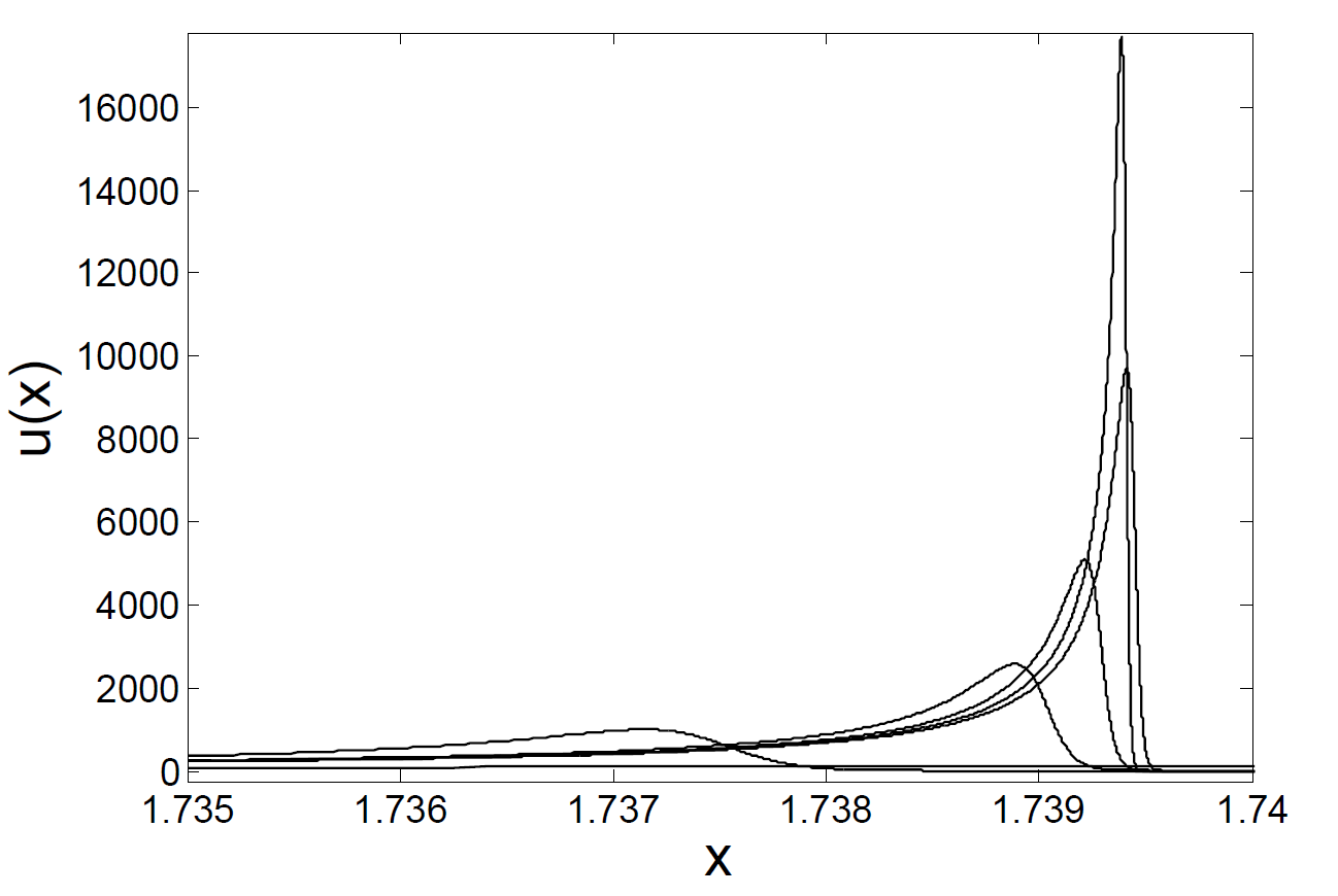
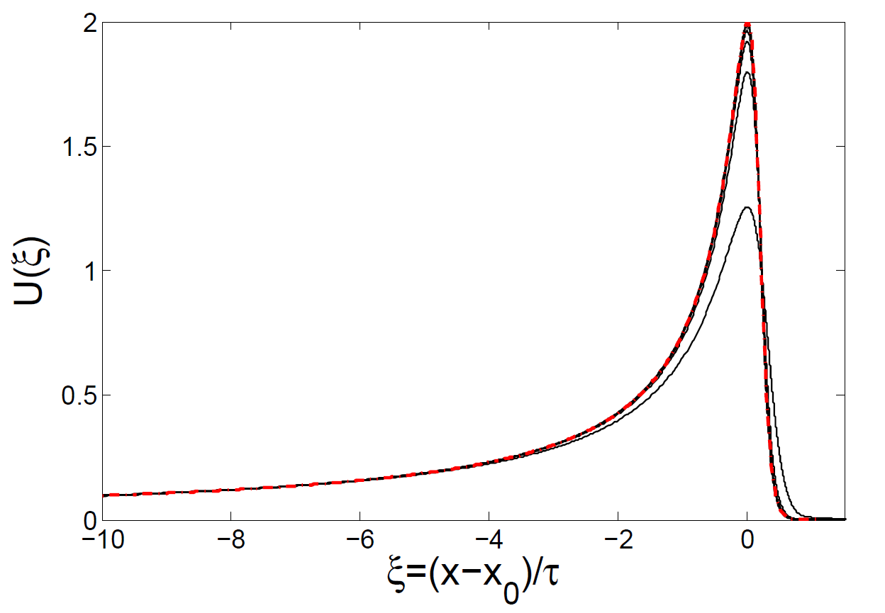
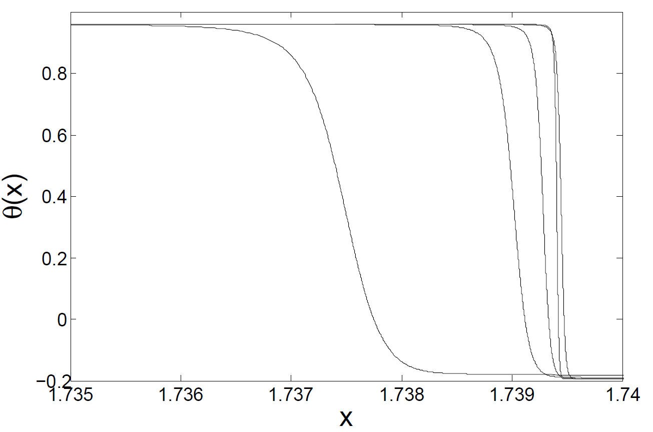
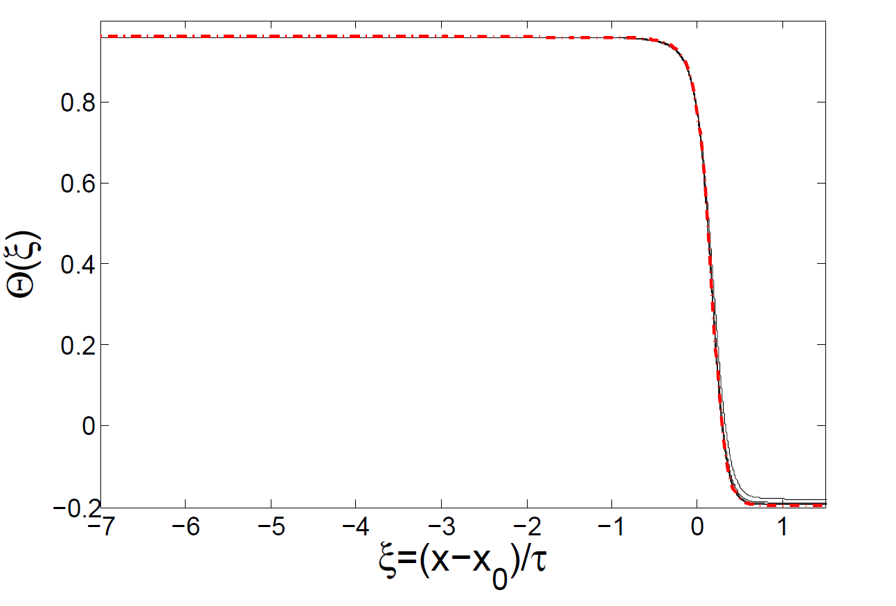
Figure 6: Similarity description of the pinch region. Five snapshots of the velocity (first row) and temperature (second row) profiles taken at times $t_{1}=4.032,\,t_{2}=5.138,\,t_{3}=5.987,\,t_{4}=6.800,\,t_{5}=7.6410$ (black lines). On the left, numerical solution using the same simulation as in Fig. 1. On the right, profiles have been rescaled according to (20), with exact solutions (33) and (44) (red dash-dotted lines) superimposed.

The temperature profile is found from (25) and (33) to be

$$\Theta_{p}=\left\{\begin{array}[]{ll}\theta_{l}-\frac{j_{0}C_{+}}{\cal M}\sqrt{\cal P}\left(\frac{\sqrt{\cal P}^{-1}-w}{4\sqrt{\cal P}-w}\right)^{\frac{4{\cal P}}{4{\cal P}-1}}&\mbox{for }{\cal P}\not=\frac{1}{4},\\ \theta_{l}-\frac{j_{0}C_{+}}{2\cal M}\exp\left\{\frac{2}{w-2}\right\}&\mbox{for }{\cal P}=\frac{1}{4}.\end{array}\right.$$ (44)

In Fig. 6, the similarity description (20) of the pinch region is tested against a typical numerical simulation of the original system (2). On the left, we show the raw data close to the pinch point $x_{0}$, while rescaled profiles are shown on the right. Once sees very good convergence toward the exact solutions (33) and (44), which are shown as the red dash-dotted lines.

By taking the limit $w\rightarrow-\infty$, which corresponds to $\xi\rightarrow\infty$, we find the following condition on the jump of the temperature across the pinch-off (see Fig. 2):

$$\theta_{r}=\theta_{l}-\frac{j_{0}C_{+}}{\cal M}\sqrt{\cal P}<\theta_{l},\quad\forall\ {\cal P}>0;$$ (45)

in particular, it shows that necessarily $\theta_{r}<\theta_{l}$. It is thus seen from (40) that $H_{p}$ grows exponentially, which does not match the drop profile, which has a finite slope (19). This means we need another region between the pinch region II and the drop IV, which we call as the transition region.

3.4 III: transition region

Here we use the same similarity form (20) as before, but the balance is different. On account of flux conservation, we have $\alpha_{1}+\alpha_{2}=1$ as before. We also require the transitional solution to match onto the linear drop profile for $\xi\rightarrow\infty$, which implies that $\alpha_{1}=\beta$. Finally, we expect surface tension to enter the force balance (2b), so that from a balance between surface tension and viscous forces we have $\alpha_{1}-3\beta=\alpha_{2}-2\beta$. From these conditions we deduce the exponents $\alpha_{1}=1$, $\alpha_{2}=0$, and $\beta=1$, and the similarity solution becomes

$$h(x,t)=\tau H_{t}\left(\xi\right),\quad u(x,t)=U_{t}\left(\xi\right),\quad\theta(x,t)=\Theta_{t}\left(\xi\right),\quad\xi=\frac{x-x_{1}(t)}{\tau},$$ (46)

where $x_{1}(t)$ denotes the center of the transition region, which will be shown below to be slightly different from the pinch point $x_{0}$. The similarity equations corresponding to (46) are

$$j_{0} =H_{t}U_{t}$$ (47a)

$$0 =H_{t}^{\prime\prime\prime}-4{\cal O}\frac{(U_{t}^{\prime}H_{t})^{\prime}}{H_{t}}$$ (47b)

$$0 =\left(H_{t}\Theta_{t}^{\prime}\right)^{\prime}.$$ (47c)

Here in the force balance (47b), only surface tension and viscosity come in at leading order $O(\tau^{-2})$.

Once more, we insert $U_{t}^{\prime}=-j_{0}H_{t}^{\prime}/H_{t}^{2}$ into (47b) and integrate once, to obtain

$$C_{3}=H_{t}^{\prime\prime}H_{t}-\frac{H_{t}^{\prime 2}}{2}-4{\cal O}j_{0}\frac{H_{t}^{\prime}}{H_{t}}.$$ (48)

For (47c) to be consistent with a general $H_{t}$-profile, $\Theta=\theta_{r}$ must be a constant, which is consistent with (45), where we matched the temperature profile in the pinch region directly to the constant value $\theta_{r}$. In order to match to the constant slope (19) for $\xi\rightarrow\infty$, we must have $H_{t}\approx s\xi$ for $\xi\rightarrow\infty$, and thus $C_{3}=-s^{2}/2$.

Rescaling (48) according to

$$H_{t}=\frac{8{\cal O}j_{0}}{\sqrt{2}s}f\left(\zeta\right),\quad\zeta=\frac{s^{2}}{8{\cal O}j_{0}}\xi,$$ (49)

it turns into

$$-1=f^{\prime\prime}f-f^{\prime 2}/2-f^{\prime}/f.$$ (50)

Putting $p(f)=f^{\prime}$, the phase plane representation of (50) is

$$p^{\prime}=\frac{p}{2f}+\frac{1}{f^{2}}-\frac{1}{pf}.$$ (51)

In order to match to (40), $H_{t}$ must behave exponentially for $\xi\rightarrow-\infty$, which means that $p\sim f$ near the origin of the $p-f$ plane. On the other hand, for $\xi\rightarrow\infty$ we have seen that $H_{t}\approx s\xi$, and so $p\approx\sqrt{2}$ for $f\rightarrow\infty$.

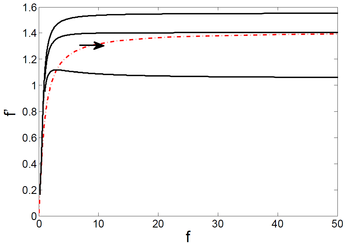
Figure 7: Phase-plane portrait of the ODE (51). The solid lines correspond to the orbits and the red dash-dotted line is the nullcline $p=0$.

The nullcline $p^{\prime}=0$ is the curve

$$f=\frac{p}{1-p^{2}/2},$$ (52)

which is shown in the phase portrait, Fig. 7, together with some typical solutions of (51). An inspection of the phase plane reveals that that there is a unique orbit that approaches the nullcline asymptotically as $f\rightarrow\infty$. As seen from (52), this is the solution that has the right asymptotics for $f\rightarrow\infty$.

For the solutions shown in Fig. 7 a more careful analysis at the origin of the phase plane is necessary. Assuming a regular expansion yields the series

$$p=f+\frac{f^{3}}{2}+\dots\equiv p_{0}(f),$$

which has no free parameters. To find the missing degree of freedom, we put $p(f)=p_{0}(f)+\delta(f)$, and linearize in $\delta$ to find

$$\delta^{\prime}=\delta\left(\frac{2}{f}-\frac{p_{0}^{\prime}}{p_{0}}+\frac{1}{p_{0}f^{2}}\right)\approx\frac{\delta}{f^{3}},$$ (53)

for small $f$. Making the WKB ansatz

$$\delta=\delta_{0}e^{-Af^{\alpha}+\dots},$$

a leading-order balance as $f\rightarrow\infty$ yields $\alpha=-2$ and $A=1/2$. Thus close to the origin, we arrive at the representation

$$p=f+\frac{f^{3}}{2}+\dots+\delta_{0}e^{-\frac{1}{2f^{2}}},$$ (54)

where the degree of freedom is in the parameter $\delta_{0}$. Now one can solve (51) by shooting from the origin to infinity, as shown in Fig. 7. The value of $\delta$ is varied until the solution asymptotes to the correct value $p=\sqrt{2}$.

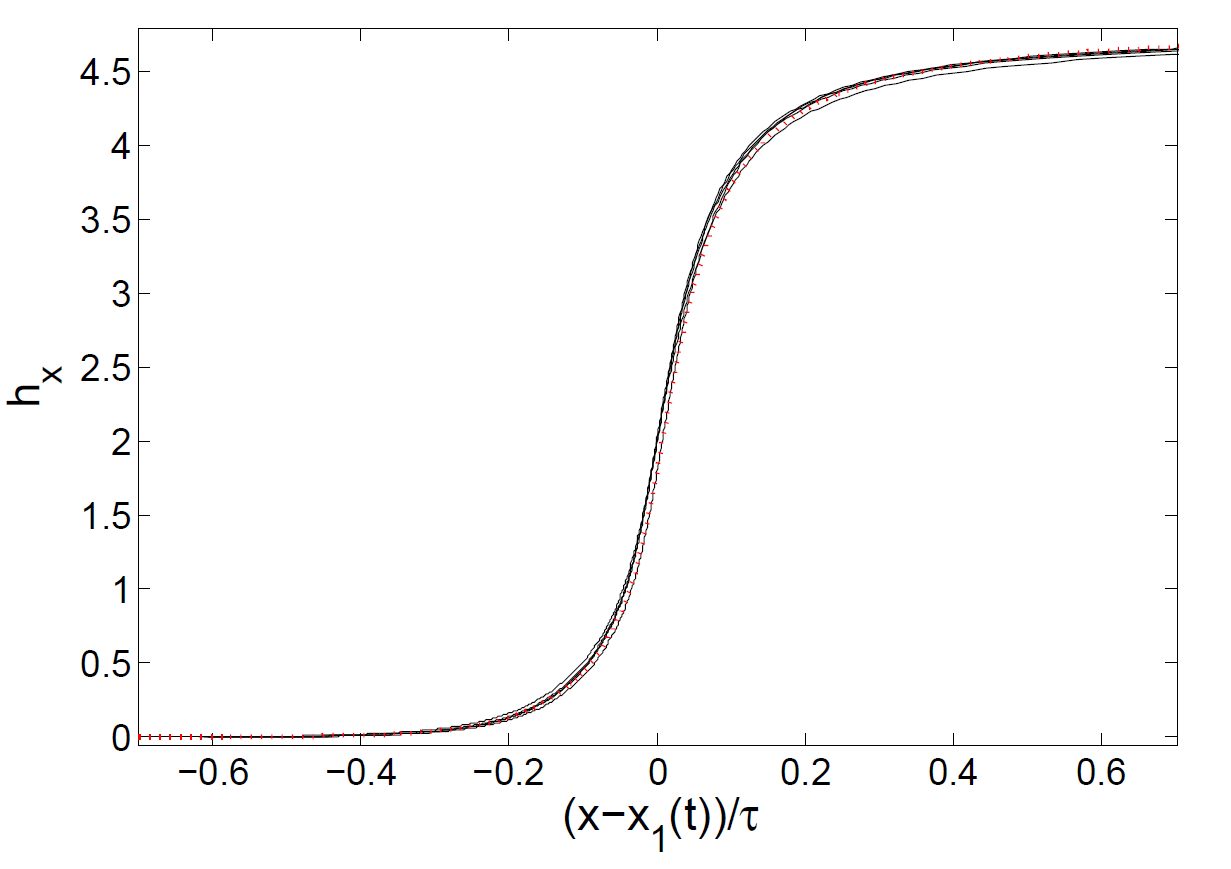
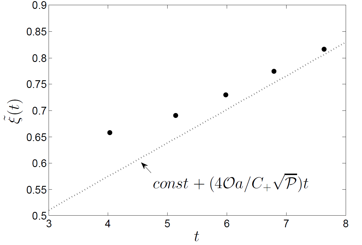
Figure 8: Similarity description of the transition region. Left: five snapshots of the spatial derivative of the height profile $h_{x}(x,t)=H_{t}^{\prime}(\xi)$, using the same simulation as in Fig. 1, for times $t_{1}=4.032,\,t_{2}=5.138,\,t_{3}=5.987,\,t_{4}=6.800,\,t_{5}=7.6410$ (black lines). Data from the transition region is shown in self-similar variables (46). Each curve is shifted such that $H_{t}^{\prime}(0)=2$, which defines $x_{1}(t)$; the collapsed profiles are compared to the solution of (48) (red dotted line), obtained by the shooting method. Right: the corresponding values of $\tilde{\xi}_{i}=(x_{1}(t_{i})-x_{0})/\tau(t_{i}),\ i=1,...,5$ (dots) compared to the prediction (59) (dotted line). The value of $a$ is taken from Fig. 3.

Once we have obtained $p(f)=f^{\prime}(\zeta)$, we find $f(\zeta)$ by (numerical) integration and thus $H_{t}(\xi)$ from (49). The derivative $H_{t}^{\prime}(\xi)$ is shown on the left of Fig. 8 as the red dotted line, and compared to $h_{x}$, as found from a numerical simulation of the full system (2). Allowing for a horizontal shift (which determines $x_{1}(t)$, see below), excellent agreement is found.

For small $f$ ($\xi\rightarrow-\infty$), $f^{\prime}=f$ yields

$$f\approx f_{0}e^{\zeta}=f_{0}e^{\frac{s^{2}}{8{\cal O}j_{0}}\xi};$$

which transforms to the asymptotics

$$H_{t}\approx Be^{\frac{s^{2}}{8{\cal O}j_{0}}\xi}\quad\text{and}\quad U_{t}\approx\frac{j_{0}}{B}e^{-\frac{s^{2}}{8{\cal O}j_{0}}\xi}\quad\text{as}\ \xi\rightarrow-\infty,$$ (55)

as well as

$$u(x,t)\approx\frac{j_{0}}{B}\exp\left\{{-\frac{s^{2}}{8{\cal O}j_{0}}\frac{x-x_{1}(t)}{\tau(t)}}\right\}$$ (56)

in the original variables. Comparing to the asymptotics in the pinch-off region (41), we find the following matching conditions:

$$C_{+} = \frac{s^{2}}{2j_{0}\sqrt{\cal P}},$$ (57)

$$B = \frac{j_{0}}{C_{+}},$$ (58)

$$\tilde{\xi}(t)=\frac{x_{1}(t)-x_{0}}{\tau(t)} = \frac{\log(\tau(t))}{C_{+}\sqrt{\cal P}}=\log\tau_{0}+\frac{4{\cal O}a}{C_{+}\sqrt{\cal P}}t>0,$$ (59)

where in the last equality in (59) we have used (9). On the right of Fig. 8 we test (59), shown as the dotted line, against the shift $x_{1}(t)$, as obtained from a direct numerical simulation (dots). For large times, the dots are seen to approach the theoretical prediction.

4 Discussion and conclusions

In this study we have derived the leading order analytical structure of self-similar solutions describing the thermal rupture of a thin viscous liquid sheet, and provided a consistent matching of them to the outer solutions. The leading order solutions in the film region are given by the velocity and height profiles (12) and (14), respectively. The film thins exponentially according to (9), while the macroscopic drop to its right has a parabolic profile (17)–(18), with no flow inside. We derived explicit formulas for the self-similar solutions (33)–(36) and (44) in the pinch region, and analyzed the solution (55) in the transitional layer. Finally, the matching conditions (19), (45) and (57)–(58) fix all the parameters of the problem in terms of $a$ and $j_{0}$. Since $j_{0}$ can be normalized to any value by choosing the origin of the time axis, the thinning rate $a$ is really the only unknown parameter. We have checked numerically that $a$ indeed depends on the fine details of the initial data and, therefore, can only be inferred from a more refined analysis.

Table 1 shows the dependence of rupture parameters upon variation of the dimensionless groups of the problem; the initial data are held fixed. The parameter $a$, and thus the pinch position $x_{0}$ varies considerably. In turn, table 2 shows dependence of parameters upon variation of initial data while keeping dimensionless groups fixed. In both tables the thinning rate $a$ was determined numerically from the asymptotic value of the quantity

$$\frac{\bar{u}^{2}}{4\cal O}-\frac{\bar{u}^{\prime\prime}\bar{u}}{\bar{u}^{\prime}}+\bar{u}^{\prime},$$

as suggested by (9). The parameter $\tau_{0}$ was fixed (similar to Fig. 3) so that $h_{f}(0)=1$, which fixes $j_{0}=4{\cal O}\sqrt{a}$. The constant $C_{+}$ was calculated by two alternative methods: using (57) with the contact angle $s$ defined by (19), or from (39). Here the maximum velocity $U_{max}$ in the pinch region was determined from $u(x,t)$, rescaled according to (20).

Table 1: Left: Dimensionless groups and macroscopic properties of three numerical simulations; initial data for all simulations is as in Fig. 1, with $M=\pi$ and $Q=-0.2\pi$. Right: rupture parameters as calculated from the analytical formulas derived for them. The temperature jump condition (45) and the formula for the position of the pinch point (15) are satisfied to within an accuracy of $5\cdot 10^{-3}$.

${\cal O}$	${\cal D}$	${\cal M}$	$U_{max}$	$\theta_{l}$	$\theta_{r}=Q/M$
0.25	0.25	10.0	2.0	0.958	-0.195
0.125	0.125	10.0	3.68	0.98	-0.195
0.25	0.25	20.0	4.121	0.882	-0.195

$a$	$j_{0}$	$C_{+}$	$\theta_{l}-\theta_{r}$	$x_{0}$
0.819	0.905	12.70	1.149	1.736
1.01	0.503	23.38	1.197	1.563
0.68	0.825	26.17	1.080	1.905

Table 2: Left: Initial data and macroscopic properties of three numerical simulations, with dimensionless groups fixed at ${\cal O}=1/4,\,{\cal D}=1/4,\,{\cal M}=10$. The initial data have the same values $M=\pi$ and $Q=-0.2\pi$. Right: rupture parameters as calculated. Both (45) and (15) are satisfied to within an accuracy of $5\cdot 10^{-3}$.

$U_{max}$	$\theta_{l}$	$\theta_{r}=Q/M$	$h(x,0)$	$u(x,0)$	$\theta(x,0)$
1.581	0.953	0.0056	1.0	$\pi\sin(x)$	$\cos(x)$
1.495	0.909	0.0051	1.0	0.0	$\cos(x)$
1.792	0.955	-0.0949	$1-0.2\cos(x)$	$\pi\sin(x)$	$\cos(x)$

$a$	$C_{+}$	$j_{0}$	$\theta_{l}-\theta_{r}$	$x_{0}$
0.887	10.039	0.942	0.946	1.668
0.905	9.492	0.951	0.903	1.651
0.849	11.379	0.921	1.048	1.705

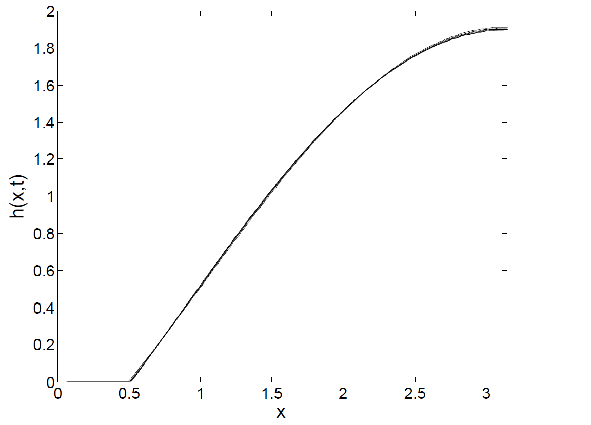
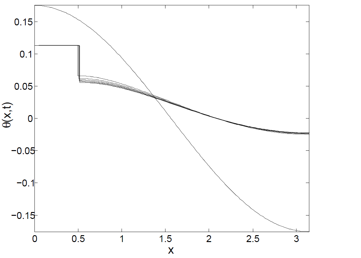
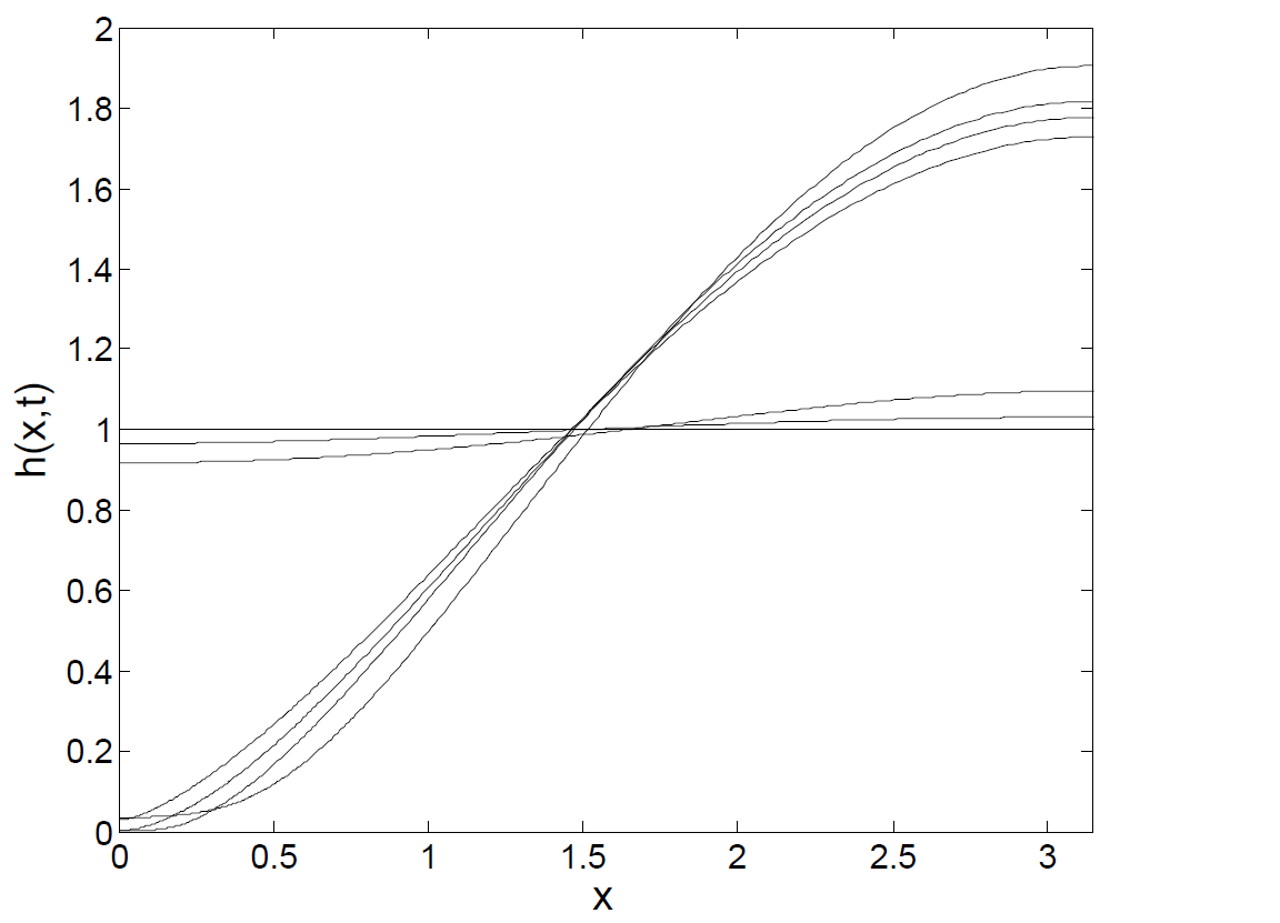
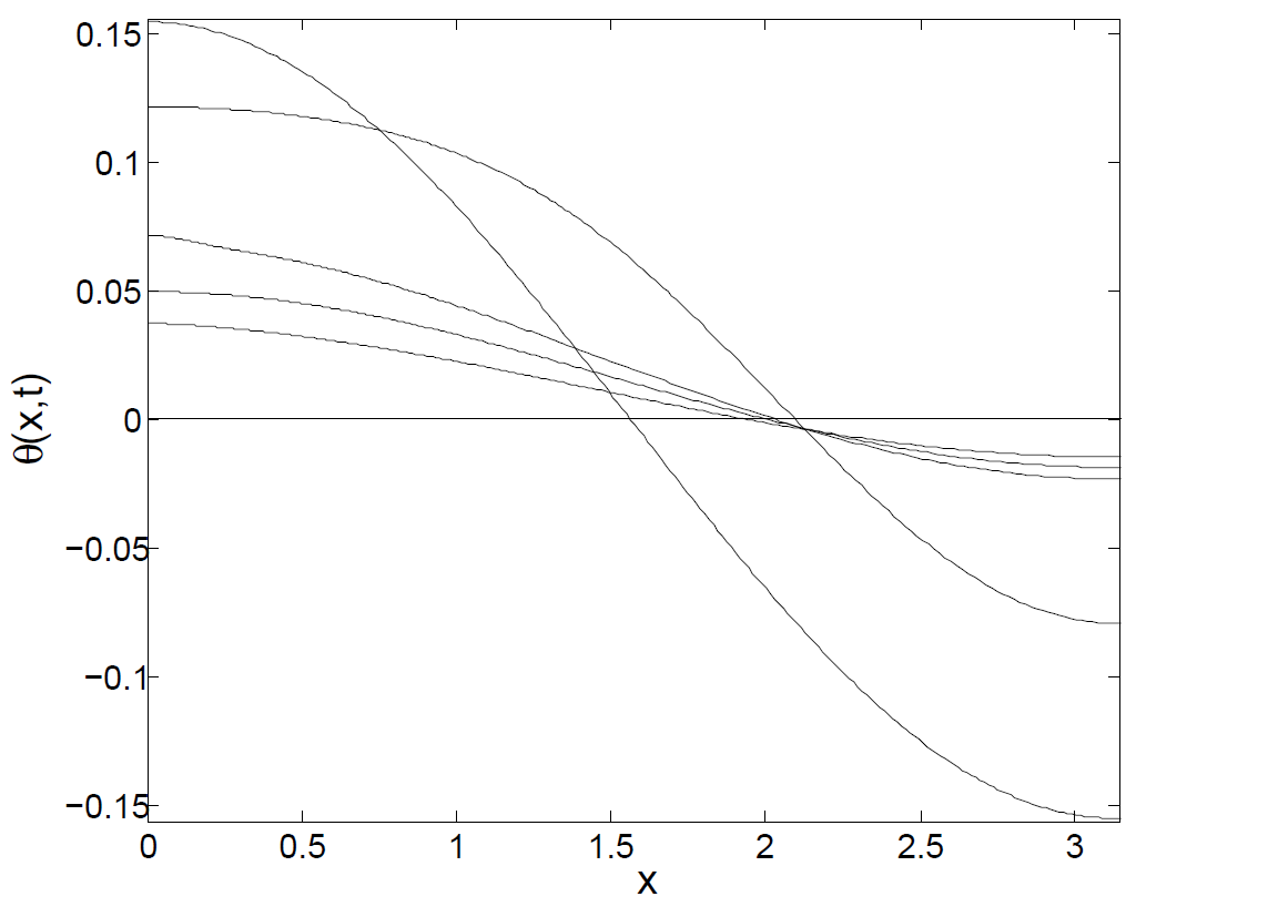
Figure 9: Plots of the height (first column) and temperature (right column) for $\Delta T=0.175>\Delta T_{cr}$ (rupture, first row) and $\Delta T=0.155<\Delta T_{cr}$ (no rupture, second row). The initial data for both simulations is given by $h(x,0)\equiv 1,\,u(x,0)\equiv 0$ and $\theta(x,\,0)=\Delta T\cos(x)$.

Since in our simulations breakup is driven by temperature gradients, it is to be expected that there exists a critical initial temperature difference above which breakup occurs, while there is no breakup below this critical value. We tested this idea using constant initial conditions $h(x,0)\equiv 1$ and $u(x,0)\equiv 0$ for the height and velocity profiles, respectively. The initial temperature profile $\theta(x,\,0)=\Delta T\sin(x+\pi/2)$ is controlled by the temperature difference $\Delta T$. Fig. 9 confirms that for $\Delta T$ smaller than a critical value $\Delta T_{cr}$, no breakup occurs, and instead both height and temperature relax toward constant values (second row). If on the other hand $\Delta T>\Delta T_{cr}$, the temperature profile develops a jump, and the height goes to zero (first row). More detailed numerical simulations indicate that $\Delta T_{cr}\approx 0.16$.

We expect a singular limiting behavior of solutions to occur when approaching the threshold $\Delta T_{cr}$ from above. The temperature plots in the first row of Fig. 9 indicate that convergence toward the self-similar solution happens more slowly as $\Delta T_{cr}$ is approached, especially inside of the droplet core. Moreover, the amplitude $\theta_{l}-\theta_{r}$ of the temperature jump, and the width of the film $(0,x_{0})$ decrease to zero as $\Delta T_{cr}\rightarrow\Delta T+0$. This suggests that the nature of the self-similar rupture changes at the critical threshold $\Delta T_{cr}$ and the rupture, if it still occurs, should happen then at the boundary of the interval $x=0$.

Finally, in Appendix A we classify all solutions to the ODE (10), which describes the velocity in the film region. In subsection 3.1 only the special solution of type $\mathrm{I}$ (according to the classification of Appendix A and Fig. 11) with $A=0$ was considered. However, our numerics indicate that for suitably chosen initial conditions (with the same boundary conditions (3)), solutions of type $\mathrm{I}$ with nonzero $A$ (an example of which is shown in Fig. 10) can be realized in the thin film region. Namely, this happens if one evolves solutions to (2) from a height profile given by a semicircle, whose maximum is located either at $x=0$ or $x=\pi$. This drop is connected to a film region given by the parts of the height profile shown in Fig. 10, taken in the intervals $x\in[-\pi/(2\sqrt{a-A^{2}}),x_{A}]$ or $x\in[x_{A},\pi/(2\sqrt{a-A^{2}})]$, respectively. Here the point $x_{A}$ is defined uniquely by the conditions

$$u(x_{A})=h^{\prime}(x_{A})=0,$$ (60)

and is chosen to be compatible with the boundary conditions (3). Correspondingly, the leading order velocity in the film region is prescribed by the corresponding parts of the type $\mathrm{I}$ solution to (61) with $|A|<\sqrt{a}$.

We conjecture that solution of types $\mathrm{II}-\mathrm{IV}$, represented in the phase portrait of Fig. 11, may also be realized in more complicated rupture scenarios, for example in the case of several pinch points separating macroscopic drops of different sizes, which interact by virtue of small fluxes through the film regions. This would be similar to systems considered recently by Clasen et al. (2006); Glasner et al. (2008) and  Kitavtsev (2014).

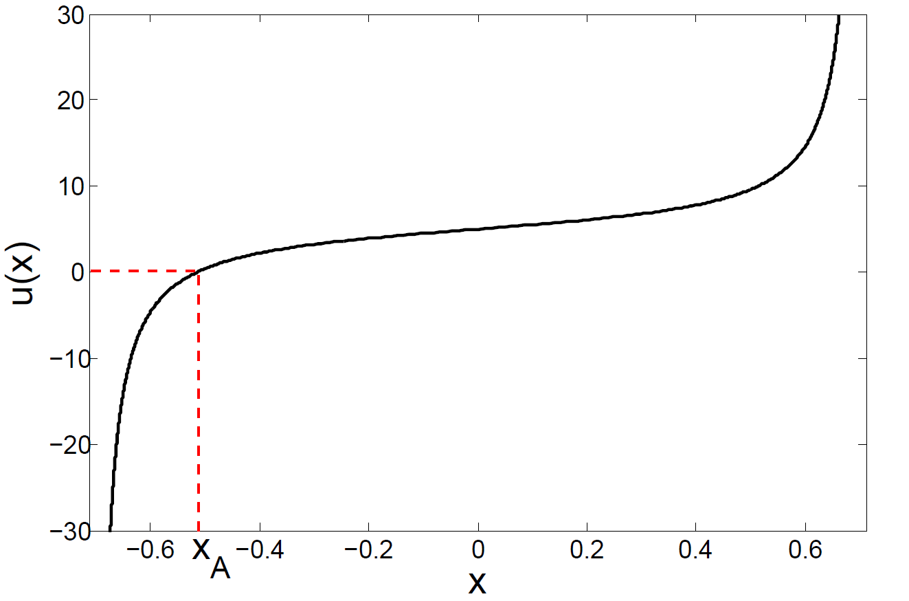
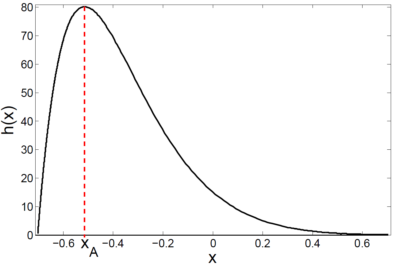
Figure 10: Velocity (left) and the corresponding height profiles (right) for the solutions to (61) in region I, defined in Fig. 11. The velocity profile was calculated using (67) for $a=30,\,A=5$. The corresponding height profiles was calculated using (13) for the flux $j_{f}=h_{f}u_{f}$. The position of the point $x_{A}$ is specified uniquely by conditions (60), and is shown by the red dashed lines.

Appendix A Analysis of the velocity equation in the film region

Here we present the solution method and phase plane analysis of the ODE (10):

$$u-\frac{a}{u}=\frac{u^{\prime\prime}}{u^{\prime}}-\frac{u^{\prime}}{u},$$ (61)

where for convenience we skipped overbars. We first reduce the order of the equation by introducing a new variable $p(u)=u^{\prime}(x)$. The corresponding equation for $p(u)$ reads

$$u-\frac{a}{u}=p^{\prime}-\frac{p}{u}.$$ (62)

By introducing $\tilde{p}=p-a$, (62) reduces to the ODE

$$u=\tilde{p}^{\prime}-\frac{\tilde{p}}{u},$$

which is invariant under the scaling $u\rightarrow Cu$ and $p\rightarrow C^{2}p$. Therefore, similar to our treatment of (28), one can apply the substitution $\tilde{p}=w(u)u^{2}$, which results in

$$1=w(u)+uw^{\prime}(u).$$

This equation can be integrated to yield

$$w(u)=-\frac{2A}{u}+1.$$

This implies that the general solution to (62) can be characterized completely by a one-parameter family of functions:

$$p(u)=(u-A)^{2}+a-A^{2}\quad\text{with}\ A\in(-\infty,\,\infty).$$ (63)

The general solution to (61) can then be obtained in the form

$$x-\bar{x}=\int\frac{du}{(u-A)^{2}+a-A^{2}},$$

which yields explicitly:

$$x-\bar{x}=\left\{\begin{array}[]{ll}\frac{1}{2\sqrt{A^{2}-a}}\log\left[\frac{u(x)-A-\sqrt{A^{2}-a}}{u(x)-A+\sqrt{A^{2}-a}}\right]&\mbox{for }|A|>\sqrt{a},\\ \frac{1}{\sqrt{a-A^{2}}}\arctan\left[\frac{u(x)-A}{\sqrt{a-A^{2}}}\right]&\mbox{for }|A|<\sqrt{a},\\ \frac{1}{A-u(x)}&\mbox{for }|A|=\sqrt{a}.\end{array}\right.$$ (67)

In particular, for solutions with $A\in(-\sqrt{a},\,\sqrt{a})$, (67) yields the explicit solution (11).

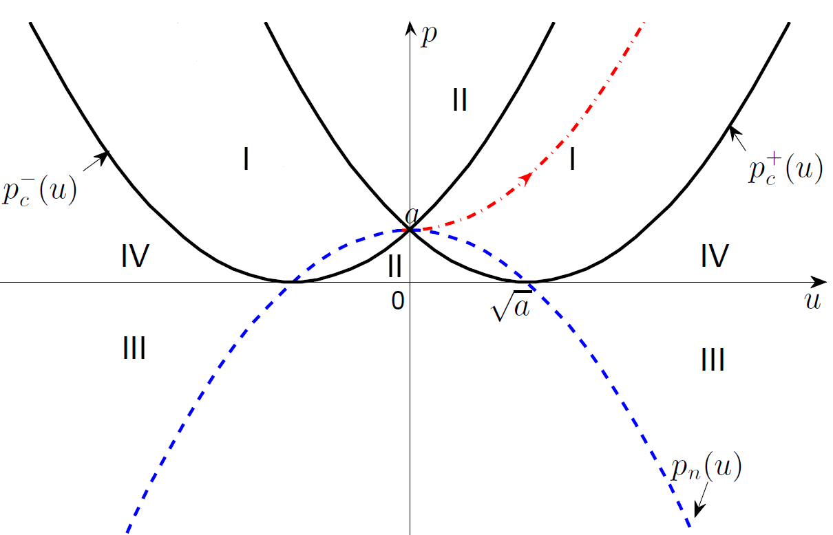
Figure 11: Phase portrait for (61). The borders of regions I-IV are defined by two parabolas $p_{c}^{\pm}(u)$ (solid black lines) and the axis $p=0$, the nullcline is defined by the parabola $p_{n}(u)$ (blue dashed line). The solution curve corresponding to (12) is shown as the dot-dashed red parabola.

To classify all solutions by phase-plane analysis, and to find their regions of existence, it is useful to write (61) as the first-order system

$$\frac{du}{dx} = p,$$

$$\frac{dp}{dx} = p\left(u-\frac{a}{u}\right)+\frac{p^{2}}{u}.$$ (68)

Firstly, owing to the invariance $p\rightarrow p$ and $u\rightarrow-u$ of (68), the phase-plane portrait is symmetric around the axis $u=0$. Moreover, all integral curves (63) intersect at the singular point $(u=0,\,p=a)$. The set of stationary points of (68) is given by the axis $p=0$, while the nullcline $dp/dx=0$ is given by the parabola

$$p_{n}(u)=a-u^{2}.$$

Correspondingly, the integral curves (63) attain their minima at the nullcline. Moreover, the axis $p=0$, together with two parabolas

$$p_{c}^{\pm}(u)=(u\pm\sqrt{a})^{2},$$

divide the phase plane into four regions shown as I-IV in Fig. 11. A solution to (61) starting in one of the regions I-IV stays in that region for all $x$.

For pinch solutions considered in this article, only those lying in region I, characterized by $A\in(-\sqrt{a},\,\sqrt{a})$ in (67) and having the explicit representation (11), are relevant. By making the shift $\bar{x}=0$ these solutions are defined in the finite interval $x\in(-\pi/(2\sqrt{a-A^{2}}),\pi/(2\sqrt{a-A^{2}}))$. They satisfy

$$u_{A}(\bar{x})=u_{A}(0)=A,$$ (69)

and tend to infinity as $x\rightarrow\pm\pi/(2\sqrt{a-A^{2}})$. These two points would correspond to pinch-off points of the full solutions to PDE system (2). The special solution (12) analyzed in Subsection 3.1 corresponds to A=0, and is selected by the global boundary conditions (3) to system (2), consistent with (69).

Solutions lying in regions II-IV are parameterized by constants $|A|>\sqrt{a}$. From the explicit representation (67) it follows that solutions in region III are defined on the whole real line $x\in\mathbb{R}\,$, while solutions in regions II and IV are defined on the half-lines $x\in(0,\,\infty)$ and $x\in(-\infty,\,0)$, respectively. In region III solutions are bounded and approach stationary points $u=A\pm\sqrt{A^{2}-a}$ at an exponential rate as $x\rightarrow\pm\infty$. The solutions in regions II (IV) are unbounded in the one-side limit $x\rightarrow 0+$ ($x\rightarrow 0-$) and approach the stationary point $u=A-\sqrt{A^{2}-a}$ ($u=A+\sqrt{A^{2}-a}$) as $x\rightarrow\infty$ ($x\rightarrow-\infty$).

References

- Bertozzi et al. (1994) Bertozzi, A. L., Brenner, M. P., Dupont, T. F. & Kadanoff, L. P. 1994 Singularities and similarities in interface flows. In Applied Mathematics Series Vol. 100 (ed. L. Sirovich), p. 155. Springer: New York.
- Boulton-Stone & Blake (1993) Boulton-Stone, J. M. & Blake, J. R. 1993 Gas-bubbles bursting at a free surface. J. Fluid Mech. 254, 437–466.
- Bowen & Tilley (2013) Bowen, M. & Tilley, B. S. 2013 On self-similar thermal rupture of thin liquid sheets. Phys. Fluids 25, 102105.
- Burton & Taborek (2007) Burton, J. C. & Taborek, P. 2007 2D inviscid pinch-off: An example of self-similarity of the second kind. Phys. Fluids 19, 102109.
- Clasen et al. (2006) Clasen, C., Eggers, J., Fontelos, M. A., Li, J. & McKinley, G. H. 2006 The beads-on-string structure of viscoelastic jets. J. Fluid Mech. 556, 283.
- Craster & Matar (2009) Craster, R. V. & Matar, O. K. 2009 Dynamics and stability of thin liquid films. Rev. Mod. Phys. 81, 1131–1198.
- Duchemin et al. (2002) Duchemin, L., Popinet, S., Josserand, C. & Zaleski, S. 2002 Jet formation in bubbles bursting at a free surface. Phys. Fluids 14, 3000–3008.
- Eggers & Dupont (1994) Eggers, J. & Dupont, T. F. 1994 Drop formation in a one-dimensional approximation of the Navier-Stokes equation. J. Fluid Mech. 262, 205.
- Eggers & Fontelos (2015) Eggers, J. & Fontelos, M. A. 2015 Singularities: Formation, Structure, and Propagation. Cambridge University Press, Cambridge.
- Eggers & Villermaux (2008) Eggers, J. & Villermaux, E. 2008 Physics of liquid jets. Rep. Progr. Phys. 71, 036601.
- Feng et al. (2014) Feng, J., Roché, M., Vigolo, D., Arnaudov, L. N., Stoyanov, S. D., Gurkov, T. D., Tsutsumanova, G. G. & Stone, H. A. 2014 Nanoemulsions obtained via bubble-bursting at a compound interface. Nature Phys. 10, 606–612.
- Glasner et al. (2008) Glasner, K., Otto, F., Rump, T. & Slepjev, D. 2008 Ostwald ripening of droplets: the role of migration. Eur. J. Appl. Math 20 (1), 1–67.
- Jensen & Grotberg (1993) Jensen, O. E. & Grotberg, J. B. 1993 The spreading of heat or soluble surfactant along a thin liquid film. Phys. FLuids A 5, 58–68.
- Kitavtsev (2014) Kitavtsev, G. 2014 Coarsening rates for the dynamics of slipping droplets. Eur. J. Appl. Math 25 (1), 83–115.
- Kitavtsev & Wagner (2010) Kitavtsev, G. & Wagner, B. 2010 Coarsening dynamics of slipping droplets. J. Eng. Math. 66, 271–292.
- Lamstaes & Eggers (2017) Lamstaes, C. & Eggers, J. 2017 Arrested bubble rise in a narrow tube. J. Stat. Phys. 167, 656.
- Lhuissier & Villermaux (2011) Lhuissier, H. & Villermaux, E. 2011 Bursting bubble aerosols. J. Fluid Mech. 696, 5–44.
- Matar (2002) Matar, O. K. 2002 Nonlinear evolution of thin free viscous films in the presence of soluble surfactant. Phys. Fluids 14, 4216.
- Matsuuchi (1976) Matsuuchi, K. 1976 Instability of thin liquid sheet and its breakup. J. Phys. Soc. Japan 41, 1410–1416.
- Néel & Villermaux (2017) Néel, B. & Villermaux, E. 2017 The spontaneous puncture of thick liquid films. J. Fluid Mech. ???, ???
- Peschka (2008) Peschka, D. 2008 Self-similar rupture of thin liquid films with slippage. Ph.D. Thesis, Humboldt University of Berlin.
- Peschka et al. (2010) Peschka, D., Münch, A. & Niethammer, B. 2010 Thin-film rupture for large slip. J. Eng. Math. 66, 33–51.
- Pugh & Shelley (1998) Pugh, M. C. & Shelley, M. J. 1998 Singularity formation in thin jets with surface tension. Comm. Pure Appl. Math. 51, 733–795.
- Rowlinson & Widom (1982) Rowlinson, J. S. & Widom, B. 1982 Molecular Theory of Capillarity. Oxford: Clarendon.
- Tammisola et al. (2011) Tammisola, O., Sasaki, A., Lundell, F., Matsubara, M. & Söderberg, L. D. 2011 Stabilizing effect of surrounding gas flow on a plane liquid sheet. J. Fluid Mech. 672, 5–32.
- Thoroddsen et al. (2012) Thoroddsen, S. T., Thoraval, M.-J., Takehara, K. & Etoh, T. G. 2012 Micro-bubble morphologies following drop impacts onto a pool surface. J. Fluid Mech. 708, 469–479.
- Tilley & Bowen (2005) Tilley, B. S. & Bowen, M. 2005 Thermocapillary control of rupture in thin viscous fluid sheets. J. Fluid Mech. 541, 399–408.
- Vrij (1966) Vrij, A. 1966 Possible mechanism for the spontaneous rupture of thin, free liquid films. Discuss. Faraday Soc. 42, 23.
- Wu (1981) Wu, J. 1981 Evidence of sea spray produced by bursting bubbles. Science 212, 324–326.