Quintessence in Multi-Measure Generalized Gravity Stabilized by Gauss-Bonnet/Inflaton Coupling

Quintessence Stabilized by Gauss-Bonnet/Inflaton CouplingE. Guendelman, E. Nissimov and S. Pacheva

Eduardo Guendelman1,2,3, Emil Nissimov4, Svetlana Pacheva4

1

2

3

4

We consider a non-standard generalized model of gravity coupled to a neutral scalar “inflaton” as well as to the fields of the electroweak bosonic sector. The essential new ingredient is employing two alternative non-Riemannian space-time volume-forms (non-Riemannian volume elements, or covariant integration measure densitities) independent of the space-time metric. The latter are defined in terms of auxiliary antisymmentric tensor gauge fields, which although not introducing any additional propagating degrees of freedom, trigger a series of important features such as: (i) appearance of two infinitely large flat regions of the effective “inflaton” potential in the corresponding Einstein frame with vastly different scales corresponding to the “early” and “late” epochs of Universe’s evolution; (ii) dynamical generation of Higgs-like spontaneous symmetry breaking effective potential for the $SU(2)\times U(1)$ iso-doublet electroweak scalar in the “late” universe, whereas it remains massless in the “early” universe.

Next, to stabilize the quintessential dynamics, we introduce in addition a coupling of the “inflaton” to Gauss-Bonnet gravitational term. The latter leads to the following radical change of the form of the total effective “inflaton” potential: its flat regions are now converted into a local maximum corresponding to a “hill-top” inflation in the “early” universe with no spontaneous breakdown of electroweak gauge symmetry and, correspondigly, into a local minimum corresponding to the “late” universe evolution with a very small value of the dark energy and with operating Higgs mechanism.

04.50.Kd, 98.80.Jk, 95.36.+x, 95.35.+d, 11.30.Qc,

1 Introduction

The interplay between the cosmological dynamics and the evolution of the symmetry breaking patterns along the history of the Universe is one of the most important paradigms at the interface of particle physics and cosmology [1]. Specifically, for the present epoch’s phase of slowly accelerating Universe (dark energy domination) see [2] and for a recent general account, see [3].

Within this context, some of the main issues we will be addressing in the present contribution are:

     (i) The existence of “early” Universe inflationary phase with unbroken electro-weak symmetry;

     (ii) The “quintessential” evolution towards “late” Universe epoch with a dynamically induced Higgs mechanism;

     (iii) Stability of the “late” Universe with spontaneous electro-weak breakdown and with a very small vacuum energy density via dynamically generated cosmological constant.

Study of issues (i) and (ii) has already been initiated in Refs.[4, 5]. Our approach is based on the powerful formalism of non-Riemannian volume-forms on the pertinent spacetime manifold [6]-[9] (for further developments, see Refs.[10]). Non-Riemannian spacetime volume-forms or, equivalently, alternative generally covariant integration measure densities are defined in terms of auxiliary maximal-rank antisymmetric tensor gauge fields (“measure gauge fields”) unlike the standard Riemannian integration measure density given given in terms of the square root of the determinant of the spacetime metric. These non-Riemannian-measure-modified gravity-matter models are also called “two-measure”, or more appropriately – “multi-measure gravity theories”.

The method of non-Riemannian spacetime volume-forms has profound impact in any (field theory) models with general coordinate reparametrization invariance, such as general relativity and its extensions ([6]-[14]), strings and (higher-dimensional) membranes [15], and supergravity [16], with the following main features:

• Cosmological constant and other dimensionful constants are dynamically generated as arbitrary integration constants in the solution of the equations of motion for the auxiliary “measure” gauge fields.

• An important characteristic feature is the global Weyl-scale invariance [7] of the starting Lagrangians actions of the underlying generalized multi-measure gravity-matter models (for a similar recent approach , see also [17]). Global Weyl-scale symmetry is responsible for the absence of a “fifth force” [9]. It undergoes spontaneous breaking due to the appearance of the above mentioned dynamically generated dimensionfull intergation constants.

• Applying the canonical Hamiltonian formalism for Dirac-constrained systems shows that the auxiliary “measure” gauge fields are in fact almost “pure gauge”, which do not correspond to propagating field degrees of freedom. The only remnant of the latter are the above mentioned arbitrary integration constants, which are identified with the conserved Dirac-constrained canonical momenta conjugated to certain components of the “measure” gauge fields [13, 14].

• Applying the non-Riemannian volume-form formalism to minimal $N=1$ supergravity we arrive at a novel mechanism for the supersymmetric Brout-Englert-Higgs effect, namely, the appearance of a dynamically generated cosmological constant triggers spontaneous supersymmetry breaking and mass generation for the gravitino [16]. Applying the same non-Riemannian volume-form formalism to anti-de Sitter supergravity produces simultaneously a very large physical gravitino mass and a very small positive observable cosmological constant [16] in accordance with modern cosmological scenarios for slowly expanding universe of the present epoch [2].

• Employing two different non-Riemannian volume-forms in generalized gravity-matter models thanks to the appearance of several arbitrary integration constants through the equations of motion w.r.t. the “measure” gauge fields, we obtain a remarkable effective scalar field potential with two infinitely large flat regions [12, 13] – $(-)$ flat region for large negative values and $(+)$ flat region for large positive values of the scalar “inflaton” with vastly different energy scales – appropriate for a unified description of both the “early” and “late” Universe evolution. An intriguing feature is the existence of a stable initial phase of non-singular universe creation preceding the inflationary phase – stable “emergent universe” without “Big-Bang” [12].

In Section 2 below we describe the construction of a non-standard generalized model of gravity coupled to a neutral scalar “inflaton”, as well as to the fields of the electroweak bosonic sector, employing the formalism of non-Riemannian space-time volume forms. A crucial feature of the corresponding total effective scalar field potential with the two infinitely large flat regions is that in the $(-)$ flat region (“early” Universe) the Higgs-like scalar of the electro-weak sector remains massless (no Higgs mechanism), whereas in the $(+)$ flat region (“late” Universe) a Higgs-like effective potential is dynamically generated triggering the standard electro-weak symmetry breaking.

A slightly different version of the formalism of Section 2 is briefly discussed in Appendix A – it is inspired by Bekenstein’s idea about gravity-assisted spontaneous electro-weak symmetry breakdown [18].

Next, in Section 3 we turn to the study of the stability issue (iii) formulated above. Namely, it is desirable that the “late” Universe epoch, instead of the infinitely large $(+)$ flat region, would be described in terms of a stable minimum of the effective “inflaton” potential. To this end we will introduce an additional linear coupling of the “inflaton” to Gauss-Bonnet gravitational term.

The Gauss-Bonnet scalar density is a specific example of gravitational terms containing higher-order powers in the curvature invariants, which appear naturally as renormalization counterterms in quantized general relativity [19], as well as in the context of string theory [20].

Recently, within the standard Einstein general relativistic setting the role of Gauss-Bonnet-“inflaton” couplings with various types of functional dependence on the “inflaton” field has been extensively discussed in the cosmological context [21].

Previously, in [22] some of us have studied a simplified generalized gravity-scalar-field model based on a single non-Riemannian volume element with a linear “inflaton”-Gauss-Bonnet coupling. In the absence of Gauss-Bonnet coupling the effective “inflaton” potential possesses in this case only one infinitely long flat region with a very small height of the order of the vacuum energy density in the “late” Universe. In the presence of the Gauss-Bonnet coupling, which modifies the “inflaton” effective potential, one finds the appearance of a local minimum on top of the aforementioned flat region of the “inflaton” potential signalling stabilization of the “late” Universe evolution with very small effective cosmological constant.

Here we will extend the work in [22] by showing that the linear “inflaton”-Gauss-Bonnet coupling has a dramatic effect on the form of the total effective “inflaton” potential in the above mentioned quintessence model based on generalized multi-measure gravity-matter theories [12, 13] in the presence of the electro-weak bosonic sector [4, 5]:

      (a) Its $(-)$ flat region is now converted into a local maximum corresponding to a “hill-top” inflation in the “early” universe a’la Hawking-Hertog mechanism [23] with no spontaneous breakdown of electroweak gauge symmetry;

      (b) Its $(+)$ flat region is converted into a local stable minimum corresponding to the “late” universe evolution with a very small value of the dark energy and with operating standard Higgs mechanism.

In Appendix B we discuss a slightly different version of the formalism in Section 3, where we will add a linear “inflaton”-Gauss-Bonnet coupling already to the initial action of the globally Weyl-scale invariant multi-measure quintessence model – this is unlike the formalism of Section 3, where the linear “inflaton”-Gauss-Bonnet coupling term is added to the corresponding Einstein-frame action. Although within the formalism of Appendix B the linear “inflaton”-Gauss-Bonnet coupling does preserve the initial global Weyl-scale invariance, it exhibits a disadventage after the passage to the physical Einstein-frame since a combinantion involving one of the auxiliary “measure” gauge fields intended to remain “pure gauge” appears now as an additional propagating field-theoretic degree of freedom.

2 Quintessence from Flat Regions of the Effective Inflaton Potential

Let us consider, following [12, 4], a multi-measure gravity-matter theory constructed in terms of two different non-Riemannian volume-forms (volume elements), where gravity couples to a neutral scalar “inflaton” and the bosonic sector of the standard electro-weak model (using units where $G_{\rm Newton}=1/16\pi$):

$$S=\int d^{4}x\,\Phi(A)\Bigl{[}g^{\mu\nu}R_{\mu\nu}(\Gamma)+L_{1}(\varphi,X)+L_{2}(\sigma,X_{\sigma};\varphi)\Bigr{]}$$

$$+\int d^{4}x\,\Phi(B)\Bigl{[}U(\varphi)+L_{3}({\mathcal{A}},{\mathcal{B}})+\frac{\Phi(H)}{\sqrt{-g}}\Bigr{]}\;.$$ (1)

Here the following notations are used:

• $\Phi(A)$ and $\Phi(B)$ are two independent non-Riemannian volume elements:

  $$\Phi(A)=\frac{1}{3!}\varepsilon^{\mu\nu\kappa\lambda}\partial_{\mu}A_{\nu\kappa\lambda}\quad,\quad\Phi(B)=\frac{1}{3!}\varepsilon^{\mu\nu\kappa\lambda}\partial_{\mu}B_{\nu\kappa\lambda}\;,$$ (2)

• $\Phi(H)=\frac{1}{3!}\varepsilon^{\mu\nu\kappa\lambda}\partial_{\mu}H_{\nu\kappa\lambda}$ is the dual field-strength of an additional auxiliary tensor gauge field $H_{\nu\kappa\lambda}$ crucial for the consistency of (1).

• We are using Palatini formalism for the Einstein-Hilbert action: the scalar curvature is given by $R=g^{\mu\nu}R_{\mu\nu}(\Gamma)$, where the metric $g_{\mu\nu}$ and the affine connection $\Gamma^{\lambda}_{\mu\nu}$ are a priori independent.

• The “inflaton” Lagrangian terms are as follows:

  $$L_{1}(\varphi,X)=X-V_{1}(\varphi)\quad,\quad X\equiv-\frac{1}{2}g^{\mu\nu}\partial_{\mu}\varphi\partial_{\nu}\varphi\;,$$ (3)

  $$V_{1}(\varphi)=f_{1}\exp\{\alpha\varphi\}\quad,\quad U(\varphi)=f_{2}\exp\{2\alpha\varphi\}\;,$$ (4)

  where $\alpha,f_{1},f_{2}$ are dimensionful positive parameters.

• $\sigma\equiv(\sigma_{a})$ is a complex $SU(2)\times U(1)$ iso-doublet scalar field with the isospinor index $a=+,0$ indicating the corresponding $U(1)$ charge. Its Lagrangian reads:

  $$L_{2}(\sigma,X_{\sigma};\varphi)=X_{\sigma}-V_{0}(\sigma)e^{\alpha\varphi}\quad,\quad X_{\sigma}\equiv-g^{\mu\nu}\bigl{(}\nabla_{\mu}\sigma_{a})^{*}\nabla_{\nu}\sigma_{a}\;,$$ (5)

  where the “bare” $\sigma$-field potential is of the same form as the standard Higgs potential:

  $$V_{0}(\sigma)=\frac{\lambda}{4}\left((\sigma_{a})^{*}\sigma_{a}-\mu^{2}\right)^{2}\;.$$ (6)

  In Appendix A below we will choose a different (simpler) version of $V_{0}(\sigma)$ (72).

• The gauge-covariant derivative acting on $\sigma$ reads:

  $$\nabla_{\mu}\sigma=\Bigl{(}\partial_{\mu}-\frac{i}{2}\tau_{A}{\mathcal{A}}_{\mu}^{A}-\frac{i}{2}{\mathcal{B}}_{\mu}\Bigr{)}\sigma\;,$$ (7)

  with $\frac{1}{2}\tau_{A}$ ($\tau_{A}$ – Pauli matrices, $A=1,2,3$) indicating the $SU(2)$ generators and ${\mathcal{A}}_{\mu}^{A}$ ($A=1,2,3$) and ${\mathcal{B}}_{\mu}$ denoting the corresponding $SU(2)$ and $U(1)$ gauge fields.

• The gauge field kinetic terms in (1) are (all indices $A,B,C=(1,2,3)$):

  $$L_{3}({\mathcal{A}},{\mathcal{B}})=-\frac{1}{4g^{2}}F^{2}({\mathcal{A}})-\frac{1}{4g^{\prime\,2}}F^{2}({\mathcal{B}})\;,$$ (8)

  $$F^{2}({\mathcal{A}})\equiv F^{A}_{\mu\nu}({\mathcal{A}})F^{A}_{\kappa\lambda}({\mathcal{A}})g^{\mu\kappa}g^{\nu\lambda}\;,\;F^{2}({\mathcal{B}})\equiv F_{\mu\nu}({\mathcal{B}})F_{\kappa\lambda}({\mathcal{B}})g^{\mu\kappa}g^{\nu\lambda}\;,$$ (9)

  $$F^{A}_{\mu\nu}({\mathcal{A}})=\partial_{\mu}{\mathcal{A}}^{A}_{\nu}-\partial_{\nu}{\mathcal{A}}^{A}_{\mu}+\epsilon^{ABC}{\mathcal{A}}^{B}_{\mu}{\mathcal{A}}^{C}_{\nu}\;,\;F_{\mu\nu}({\mathcal{B}})=\partial_{\mu}{\mathcal{B}}_{\nu}-\partial_{\nu}{\mathcal{B}}_{\mu}\;.$$ (10)

The form of the action (1) is fixed by the requirement of invariance under global Weyl-scale transformations:

$$g_{\mu\nu}\to\lambda g_{\mu\nu}\;,\;\Gamma^{\mu}_{\nu\lambda}\to\Gamma^{\mu}_{\nu\lambda}\;,\;\varphi\to\varphi-\frac{1}{\alpha}\ln\lambda\;$$ (11)

$$A_{\mu\nu\kappa}\to\lambda A_{\mu\nu\kappa}\;,\;B_{\mu\nu\kappa}\to\lambda^{2}B_{\mu\nu\kappa}\;,\;H_{\mu\nu\kappa}\to H_{\mu\nu\kappa}\;,$$

and the electro-weak fields remain inert under (11).

Equations of motion for the affine connection $\Gamma^{\mu}_{\nu\lambda}$ yield a solution for the latter as a Levi-Civita connection:

$$\Gamma^{\mu}_{\nu\lambda}=\Gamma^{\mu}_{\nu\lambda}({\bar{g}})=\frac{1}{2}{\bar{g}}^{\mu\kappa}\left(\partial_{\nu}{\bar{g}}_{\lambda\kappa}+\partial_{\lambda}{\bar{g}}_{\nu\kappa}-\partial_{\kappa}{\bar{g}}_{\nu\lambda}\right)\;,$$ (12)

w.r.t. to the Weyl-conformally rescaled metric ${\bar{g}}_{\mu\nu}$:

$${\bar{g}}_{\mu\nu}=\chi_{1}g_{\mu\nu}\quad,\quad\chi_{1}\equiv\frac{\Phi_{1}(A)}{\sqrt{-g}}\;.$$ (13)

The metric ${\bar{g}}_{\mu\nu}$ plays an important role as the “Einstein frame” metric (see (18) below).

Variation of the action (1) w.r.t. auxiliary tensor gauge fields $A_{\mu\nu\lambda}$, $B_{\mu\nu\lambda}$ and $H_{\mu\nu\lambda}$ yields the equations:

$$\partial_{\mu}\Bigl{[}R+L_{1}(\varphi,X)+L_{2}(\sigma,X_{\sigma};\varphi)\Bigr{]}=0\quad,$$ (14)

$$\partial_{\mu}\Bigl{[}U(\varphi)+L_{3}({\mathcal{A}},{\mathcal{B}})+\frac{\Phi(H)}{\sqrt{-g}}\Bigr{]}=0\quad,\quad\partial_{\mu}\Bigl{(}\frac{\Phi_{2}(B)}{\sqrt{-g}}\Bigr{)}=0\;,$$ (15)

whose solutions read:

$$\frac{\Phi_{2}(B)}{\sqrt{-g}}\equiv\chi_{2}={\rm const}\;\;,\;\;R+L_{1}(\varphi,X)+L_{2}(\sigma,X_{\sigma};\varphi)=M_{1}={\rm const}\;,$$

$$U(\varphi)+L_{3}({\mathcal{A}},{\mathcal{B}})+\frac{\Phi(H)}{\sqrt{-g}}=-M_{2}={\rm const}\;.$$ (16)

Here $M_{1}$ and $M_{2}$ are arbitrary dimensionful and $\chi_{2}$ arbitrary dimensionless integration constants. We will take all $M_{1,2},\,\chi_{2}$ to be positive.

The first integration constant $\chi_{2}$ in (16) preserves global Weyl-scale invariance (11) whereas the appearance of the second and third integration constants $M_{1},\,M_{2}$ signifies dynamical spontaneous breakdown of global Weyl-scale invariance under (11) due to the scale non-invariant solutions (second and third ones) in (16).

It is important to elucidate the physical meaning of the three arbitrary integration constants $M_{1},\,M_{2},\,\chi_{2}$ from the point of view of the canonical Hamiltonian formalism. Namely, as shown in [4], the auxiliary maximal rank antisymmetric tensor gauge fields $A_{\mu\nu\lambda},B_{\mu\nu\lambda},H_{\mu\nu\lambda}$ entering the original non-Riemannian volume-form action (1) do not correspond to additional propagating field-theoretic degrees of freedom. The integration constants $M_{1},\,M_{2},\,\chi_{2}$ are the only dynamical remnant of the latter and they are identified as conserved Dirac-constrained canonical momenta conjugated to (certain components of) $A_{\mu\nu\lambda},B_{\mu\nu\lambda},H_{\mu\nu\lambda}$.

Following [12, 4] we first find from (16) the expression for $\chi_{1}$ (13) as algebraic function of the scalar matter fields:

$$\frac{1}{\chi_{1}}=\frac{1}{2\chi_{2}}\,\frac{V_{1}(\varphi)+V_{0}(\sigma)e^{\alpha\varphi}+M_{1}}{U(\varphi)+M_{2}}\;.$$ (17)

Then we perform transition from the original metric $g_{\mu\nu}$ to ${\bar{g}}_{\mu\nu}$ arriving at the “Einstein-frame” formulation, where the gravity equations of motion are written in the standard form of Einstein’s equations:

$$R_{\mu\nu}({\bar{g}})-\frac{1}{2}{\bar{g}}_{\mu\nu}R({\bar{g}})=\frac{1}{2}T^{\rm eff}_{\mu\nu}$$ (18)

originating from the Einstein-frame action:

$$S_{\rm EF}=\int d^{4}x\sqrt{-{\bar{g}}}\Bigl{[}R({\bar{g}})+L_{\rm eff}\bigl{(}\varphi,{\bar{X}},\sigma,{\bar{X}}_{\sigma},{\mathcal{A}},{\mathcal{B}}\bigr{)}\Bigr{]}\;,$$ (19)

with the effective energy-momentum tensor $T^{\rm eff}_{\mu\nu}$ given in terms of the Einstein-frame matter Lagrangian $L_{\rm eff}$:

$$L_{\rm eff}={\bar{X}}+{\bar{X}}_{\sigma}-U_{\rm eff}\bigl{(}\varphi,\sigma\bigr{)}-\frac{\chi_{2}}{4g^{2}}{\bar{F}}^{2}({\mathcal{A}})-\frac{\chi_{2}}{4g^{\prime\,2}}{\bar{F}}^{2}({\mathcal{B}})\;.$$ (20)

Here bars indicate that the quantities are given in terms of the Einstein-frame metric (13), e.g., ${\bar{X}}\equiv-\frac{1}{2}{\bar{g}}^{\mu}\nu\partial_{\mu}\varphi\partial_{\nu}\varphi$ , ${\bar{X}}_{\sigma}\equiv-{\bar{g}}^{\mu\nu}\bigl{(}\nabla_{\mu}\sigma_{a})^{*}\nabla_{\nu}\sigma_{a}$ etc, and the total scalar field effective potential reads:

$$U_{\rm eff}\bigl{(}\varphi,\sigma\bigr{)}=\frac{\Bigl{(}V_{1}(\varphi)+V_{0}(\sigma)e^{\alpha\varphi}+M_{1}\Bigr{)}^{2}}{4\chi_{2}(U(\varphi)+M_{2})}$$

$$=\frac{\Bigl{(}M_{1}e^{-\alpha\varphi}+f_{1}+\frac{\lambda}{4}\left((\sigma_{a})^{*}\sigma_{a}-\mu^{2}\right)^{2}\Bigr{)}^{2}}{4\chi_{2}(M_{2}e^{-2\alpha\varphi}+f_{2})}$$ (21)

(see Eq.(73) below for the Bekenstein-inspired form of $V_{0}(\sigma)$ (72)).

A remarkable feature of the effective scalar potential $U_{\rm eff}(\varphi,\sigma)$ (21) is that it possesses two infinitely large flat regions describing the “early” and “late” Universe, respectively (see (26) and (28) below):

• (-) flat region – for large negative values of $\varphi$, where:

  $$U_{\rm eff}(\varphi,\sigma)\simeq U_{(-)}\equiv\frac{M_{1}^{2}}{4\chi_{2}\,M_{2}}\;.$$ (22)

  In this region the Higgs-like field $\sigma$ remains massless and there is no spontaneous breakdown of electro-weak gauge symmetry.

• (+) flat region – for large positive values of $\varphi$, where:

  $$U_{\rm eff}(\varphi,\sigma)\simeq U_{(+)}(\sigma)=\frac{\Bigl{(}\frac{\lambda}{4}\left((\sigma_{a})^{*}\sigma_{a}-\mu^{2}\right)^{2}+f_{1}\Bigr{)}^{2}}{4\chi_{2}\,f_{2}}\;,$$ (23)

  which obviously yields as a lowest lying vacuum the Higgs one $|\sigma|=\mu$ with a residual effective cosmological constant $\Lambda_{(+)}$:

  $$2\Lambda_{(+)}\equiv U_{(+)}(\mu)=\frac{f_{1}^{2}}{4\chi_{2}f_{2}}\;.$$ (24)

  For the Bekenstein-inspired form of $U_{(+)}(\sigma)$, see Eq.(75) below.

Choosing the scales of the original “inflaton” coupling constants $f_{1,2}$ in terms of fundamental physical constants as:

$$f_{1}\sim M^{4}_{EW}\quad,\quad f_{2}\sim M^{4}_{Pl}\;,$$ (25)

where $M_{EW},\,M_{Pl}$ are the electroweak and Plank scales, respectively, we are then naturally led to a very small vacuum energy density in the (+) flat region (24):

$$U_{(+)}(\mu)\sim M^{8}_{EW}/M^{4}_{Pl}\sim 10^{-122}M^{4}_{Pl}\;,$$ (26)

which is the right order of magnitude for the present epoch’s (“late” Universe) vacuum energy density as already realized in [24].

On the other hand, if we take the order of magnitude of the integration constants

$$M_{1}\sim M_{2}\sim 10^{-8}M_{Pl}^{4}\;,$$ (27)

then the order of magnitude of the vacuum energy density in the (-) flat region (22) becomes:

$$U_{(-)}\sim M_{1}^{2}/M_{2}\sim 10^{-8}M_{Pl}^{4}\;,$$ (28)

which conforms to the Planck Collaboration data [25] for the “early” Universe’s energy scale of inflation being of order $10^{-2}M_{Pl}$.

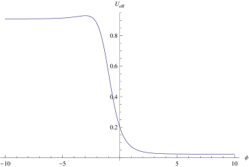
Figure 1: Qualitative shape of the effective “inflaton” potential $U_{\rm eff}$ (21) as function of $\varphi$ (for fixed $\sigma$) before inflaton coupling to Gauss-Bonnet term.

Let us note the small “bump” on the l.h.s. of the graph (Fig.1) of $U_{\rm eff}$ (21) as function of $\varphi$ and where $|\sigma_{\rm vac}|=0$ – this is a local maximum located towards the end of the $(-)$ flat region at $\varphi=\varphi_{\rm max}$:

$$e^{-\alpha\varphi_{\rm max}}=\frac{M_{1}f_{2}}{M_{2}f_{1}(\mu)}\quad,\quad f_{1}(\mu)\equiv f_{1}+\lambda\mu^{4}/4\;.$$ (29)

We note that the relative height $\Delta U_{(-)}$ of the above mentioned “bump” of the inflaton potential (21) (at $|\sigma_{\rm vac}|=0$) w.r.t. the height of the $(-)$ flat region (22):

$$\Delta U_{(-)}\equiv U_{\rm eff}(\varphi_{\rm max},0)-\frac{M_{1}^{2}}{4\chi_{2}M_{2}}=\frac{f_{1}^{2}(\mu)}{4\chi_{2}f_{2}}$$ (30)

is of the same order of magnitude as the small effective cosmological constant (24) in the $(+)$ flat region (“late” Universe) (recall $f_{1}\sim M_{EW}$, $\mu\sim M_{EW}$ and the bare Higgs-like dimensionless self-coupling $\lambda$ being small).

On the other hand, the inflaton potential (21) at $|\sigma|=|\sigma_{\rm vac}|=\mu$ does not possess a strict minimum on the $(+)$ flat region – the strict minimum occurs formally at $\varphi\to+\infty$. In the next Section we will see how adding a coupling of the inflaton to a gravitational Gauss-Bonnet density will convert the infinitely large $(+)$ flat region of the effective inflaton potential into a region with a stable minimum. Simultaneously, the infinitely large $(-)$ flat region of the effective inflaton potential with the small “bump” at its end (29)-(30) will be converted into a region with well-peaked maximum and sharper decent for large negative inflaton values (see Fig.3 below).

3 Adding Gauss-Bonnet/Inflaton Coupling

Let us now supplement the Einstein-frame action (19) with a linear coupling of the “inflaton” to gravitational Gauss-Bonnet term ${\mathcal{R}}_{\rm GB}$ with a (positive) coupling constant $b$:

$$S_{\rm EF}=\int d^{4}x\sqrt{-{\bar{g}}}\Bigl{[}R({\bar{g}})+{\bar{X}}+{\bar{X}}_{\sigma}-U_{\rm eff}\bigl{(}\varphi,\sigma\bigr{)}$$

$$-\frac{\chi_{2}}{4g^{2}}{\bar{F}}^{2}({\mathcal{A}})-\frac{\chi_{2}}{4g^{\prime\,2}}{\bar{F}}^{2}({\mathcal{B}})-b\,\varphi\,{\bar{\mathcal{R}}}_{\rm GB}\Bigr{]}\;,$$ (31)

with $U_{\rm eff}\bigl{(}\varphi,\sigma\bigr{)}$ as in (21), and:

$${\bar{\mathcal{R}}}_{\rm GB}={\bar{R}}_{\mu\nu\kappa\lambda}{\bar{R}}^{\mu\nu\kappa\lambda}-4{\bar{R}}_{\mu\nu}{\bar{R}}^{\mu\nu}+{\bar{R}}^{2}\;,$$ (32)

where all objects with superimposed bars are defined w.r.t. second-order formalism with the Einstein-frame metric ${\bar{g}}_{\mu\nu}$.

Here we will be interested in “vacuum” solutions, i.e., for constant values of the matter fields. The corresponding equations of motion for constant $\varphi$ and $\sigma$ read:

$${\bar{R}}_{\mu\nu}-\frac{1}{2}{\bar{g}}_{\mu\nu}{\bar{R}}=-\frac{1}{2}{\bar{g}}_{\mu\nu}U_{\rm eff}(\varphi,\sigma)\;,$$ (33)

note that the Gauss-Bonnet coupling does not contribute to the vacuum energy density on the r.h.s. of (33);

$$\frac{{\partial{}}}{{\partial{\varphi}}}U_{\rm eff}(\varphi,\sigma)+b{\mathcal{R}}_{\rm GB}=0\;;$$ (34)

$$\frac{{\partial{}}}{{\partial{\sigma_{a}}}}U_{\rm eff}(\varphi,\sigma)=0\quad\longrightarrow\quad\frac{{\partial{}}}{{\partial{\sigma_{a}}}}V_{0}(\sigma)=0\;\phantom{aaa}$$

$$\longrightarrow\quad(\sigma_{a})^{*}\left((\sigma_{a^{\prime}})^{*}\sigma_{a^{\prime}}-\mu^{2}\right)=0\;\;\longrightarrow\;\;\;|\sigma_{\rm vac}|=\mu\;\;{\mathrm{o}r}\;\;|\sigma_{\rm vac}|=0\;.$$ (35)

For constant $\varphi$ and $\sigma$ the solution to (33) is maximally symmetric:

$${\bar{R}}_{\mu\nu\kappa\lambda}=\frac{1}{6}U_{\rm eff}(\varphi,\sigma)\bigl{(}{\bar{g}}_{\mu\kappa}{\bar{g}}_{\nu\lambda}-{\bar{g}}_{\mu\lambda}{\bar{g}}_{\nu\kappa}\bigr{)}\;,$$ (36)

which yields for the Gauss-Bonnet term (32):

$${\mathcal{R}}_{\rm GB}=\frac{2}{3}\Bigl{(}U_{\rm eff}(\varphi,\sigma)\Bigr{)}^{2}\;.$$ (37)

Inserting (37) into $\varphi$-“vacuum” equation (34) we get:

$$\frac{{\partial{}}}{{\partial{\varphi}}}U_{\rm eff}(\varphi,\sigma_{\rm vac})+\frac{2b}{3}\Bigl{(}U_{\rm eff}(\varphi,\sigma_{\rm vac})\Bigr{)}^{2}=0\;,$$ (38)

with $\sigma_{\rm vac}$ as in (35). Eq.(38) implies that in fact the total effective inflaton potential after introducing Gauss-Bonnet/inflaton linear coupling is modified from $U_{\rm eff}(\varphi,\sigma_{\rm vac})$ (21) to the following one:

$$V_{\rm total}(\varphi,\sigma_{\rm vac})=U_{\rm eff}(\varphi,\sigma_{\rm vac})+\frac{2b}{3}\int^{\varphi}d\phi\Bigl{(}U_{\rm eff}(\phi,\sigma_{\rm vac})\Bigr{)}^{2}\;,$$ (39)

Eq.(38) upon inserting the explicit expression (21) acquires the form:

$$\frac{{\partial{}}}{{\partial{\varphi}}}V_{\rm total}(\varphi,\sigma_{\rm vac})=\frac{b\,M_{1}^{4}\bigl{(}e^{-\alpha\varphi}+{\widetilde{f}}_{1}/M_{1}\Bigr{)}}{24\chi_{2}^{2}M_{2}^{2}\bigl{(}e^{-2\alpha\varphi}+f_{2}/M_{2}\Bigr{)}}\,F(e^{-\alpha\varphi})=0\;,$$ (40)

$${\widetilde{f}}_{1}\equiv f_{1}+\frac{\lambda}{4}(|\sigma_{\rm vac}|^{2}-\mu^{2})^{2}=\left\{\begin{array}[]{ll}{f_{1}\quad{\mathrm{f}or}\;\;|\sigma_{\rm vac}|=\mu}\\ {f_{(}\mu)\equiv f_{1}+\frac{\lambda}{4}\mu^{4}}\quad{\mathrm{f}or}\;\;\sigma_{\rm vac}=0\end{array}\right.$$ (43)

where the “vacuum” solutions $z\equiv e^{-\alpha\varphi_{\rm vac}}$ must be real positive roots of the following cubic polynomial:

$$F(z)\equiv z^{3}+\frac{3{\widetilde{f}}_{1}}{M_{1}}\Bigl{(}1+\frac{4\alpha\chi_{2}M_{2}}{b\,M_{1}^{2}}\Bigr{)}z^{2}-\frac{3{\widetilde{f}}^{2}_{1}}{M_{1}^{2}}\Bigl{(}\frac{4\alpha\chi_{2}f_{2}}{b\,{\widetilde{f}}^{2}_{1}}-1\Bigr{)}z+\frac{{\widetilde{f}}^{3}_{1}}{M_{1}^{3}}=0\;.$$ (44)

Existence of two different positive roots of $F(z)$ (44) – $z_{0}(b)\equiv e^{-\alpha\varphi_{0}(b)}$ corresponding to a minimum of $V_{\rm total}(\varphi,\sigma_{\rm vac})$ (39), and $z_{1}(b)\equiv e^{-\alpha\varphi_{1}(b)}$ corresponding to a maximum of $V_{\rm total}(\varphi,\sigma_{\rm vac})$, where the dependence on the inflaton-Gauss-Bonnet coupling constant $b$ is explicitly indicated (cf. Fig.2 and Eqs.(51)-(53) below) – imposes the following upper limit for the parametric dependence of $\varphi_{0,1}(b)$ on $b$:

$$b<b_{\rm max}\equiv\frac{12\alpha\chi_{2}M_{2}\,Q}{M_{1}^{2}[2Q^{3}+3Q^{2}-3Q-2+2(Q^{2}+Q+1)^{3/2}]}\quad,\;\;Q\equiv\frac{M_{2}{\widetilde{f}}^{2}_{1}}{M_{1}^{2}f_{2}}\;.$$ (45)

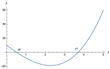
Figure 2: Qualitative plot of the cubic polynomial $F(z)$ (44).

The extremums $z_{0,1}(b)\equiv\exp\{-\alpha\,\varphi_{0,1}(b)\}$ of $V_{\rm total}(\varphi,\sigma_{\rm vac})$ (39) are given explicitly (for $0\leq b<b_{\rm max}$ (45)) as:

$$z_{0,1}(b)=\sqrt{A}\Bigl{[}\cos\bigl{(}\frac{1}{3}\arctan\sqrt{A^{3}/B^{2}-1}\bigr{)}\mp\sqrt{3}\sin\bigl{(}\frac{1}{3}\arctan\sqrt{A^{3}/B^{2}-1}\bigr{)}\Bigr{]}$$

$$-\frac{{\widetilde{f}}_{1}}{M_{1}}\Bigl{(}1+\frac{4\alpha\chi_{2}M_{2}}{b\,M_{1}^{2}}\Bigr{)}\quad,\phantom{aaaaa}$$ (46)

where the quantities $A$ and $B$ are expressed in terms of the parameters as:

$$A\equiv\frac{{\widetilde{f}}^{2}_{1}}{M^{2}_{1}}\,\omega\,\bigl{(}1+2Q+Q^{2}\omega\bigr{)}\quad,\quad\omega\equiv\frac{4\alpha\chi_{2}f_{2}}{b\,{\widetilde{f}}^{2}_{1}}\;\;,\;\;Q\;{\mathrm{a}s\leavevmode\nobreak\ in\leavevmode\nobreak\ (\ref{eq:b-limit})}\;,$$ (47)

$$B\equiv\frac{{\widetilde{f}}^{3}_{1}}{M^{3}_{1}}\,\omega\,\bigl{[}\frac{3}{2}+\frac{3}{2}Q(\omega+1)+3Q^{2}\omega+Q^{3}\omega^{2}\bigr{]}\;.$$ (48)

The condition (45) comes from the inequality $A^{3}/B^{2}-1>0$ in (46).

For $b>b_{\rm max}$ there are no real positive roots of $F(z)$ (44), and in the limiting case $b=b_{\rm max}$ the roots $z_{0,1}(b_{\rm max})\equiv\exp\{-\alpha\varphi_{0,1}(b_{\rm max})$ coalesce and become an inflex point of $F(z)$ (44):

$$z_{0}(b_{\rm max})=z_{1}(b_{\rm max})\equiv z(b_{\rm max})\quad,\quad F^{\prime}\bigl{(}z(b_{\rm max})\bigr{)}=0\;,$$ (49)

$$z(b_{\rm max})=\frac{{\widetilde{f}}_{1}}{M_{1}}\Bigl{[}\sqrt{(1+Q\omega_{\rm max})^{2}+\omega_{\rm max}-1}-(1+Q\omega_{\rm max})\Bigr{]}\;\;,$$ (50)

$$\omega_{\rm max}\equiv\frac{4\alpha\chi_{2}f_{2}}{b_{\rm max}\,{\widetilde{f}}^{2}_{1}}\;,$$

using the short-hand notations in (45), (47). In other words, for $b\geq b_{\rm max}$ there are no extremums of the total inflaton effective potential (39).

The second derivative w.r.t. $\varphi$ of $V_{\rm total}(\varphi,\sigma_{\rm vac})$ (39) at the extremums $z_{0,1}(b)\equiv\exp\{-\alpha\,\varphi_{0,1}(b)\}$ reads:

$$\frac{\partial^{2}}{\partial\varphi^{2}}V_{\rm total}(\varphi_{0,1},\sigma_{\rm vac})=-\frac{b\,\alpha z_{0,1}(b)M_{1}^{4}\bigl{(}z_{0,1}(b)+{\widetilde{f}}_{1}/M_{1}\bigr{)}}{24\chi_{2}^{2}M_{2}^{2}\bigl{(}z^{2}_{0,1}(b)+f_{2}/M_{2}\bigr{)}^{2}}\,F^{\prime}\bigl{(}z_{0,1}(b)\bigr{)}\;,$$ (51)

$$F^{\prime}\bigl{(}z_{0,1}(b)\bigr{)}=3z^{2}_{0,1}(b)+\frac{6{\widetilde{f}}_{1}}{M_{1}}\Bigl{(}1+\frac{4\alpha\chi_{2}M_{2}}{b\,M_{1}^{2}}\Bigr{)}z_{0,1}(b)\phantom{aaaaaaa}$$

$$-\frac{3{\widetilde{f}}^{2}_{1}}{M_{1}^{2}}\Bigl{(}\frac{4\alpha\chi_{2}f_{2}}{b\,{\widetilde{f}}^{2}_{1}}-1\Bigr{)}\;,\phantom{aaaaa}$$ (52)

where we have (see Fig.2):

$$F^{\prime}\bigl{(}z_{0}(b)\bigr{)}<0\quad,\quad F^{\prime}\bigl{(}z_{1}(b)\bigr{)}>0\;.$$ (53)

Taking also into account that:

$$\frac{\partial^{2}}{\partial\sigma^{2}}U_{\rm eff}(\varphi_{0}(b),\sigma_{\rm vac}=\mu)>0\quad,\quad\frac{\partial^{2}}{\partial\sigma^{2}}U_{\rm eff}(\varphi_{1}(b),\sigma_{\rm vac}=0)<0\;,$$ (54)

we conclude that (see Fig.3):

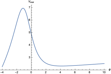
Figure 3: Qualitative shape of the total effective “inflaton” potential $V_{\rm total}(\varphi,\sigma_{\rm vac})$ (39) as function of $\varphi$ after adding inflaton coupling to Gauss-Bonnet term.

• $z_{0}(b)\equiv e^{-\alpha\varphi_{0}(b)}$ (46) with $\sigma_{\rm vac}=\mu$ (spontaneous breakdown of electro-weak symmetry) is a local stable minimum of the total inflaton effective potential (39). With the choice from Section 2 ($f_{1}\sim M^{4}_{EW}$, $f_{2}\sim M^{4}_{Pl}$, $M_{1,2}\sim 10^{-8}M^{4}_{Pl}$) we find ($b_{\rm max}$ as in (45), $z(b_{\rm max})$ as in (50)):

  $$0\leq z_{0}(b)\equiv e^{-\alpha\varphi_{0}(b)}<z(b_{\rm max})\;,$$ (55)

  where:

  $$z_{0}(b)\equiv e^{-\alpha\varphi_{0}(b)}\to 0\;\;,{\mathrm{i}.e.}\;\;\varphi_{0}(b)\to+\infty\quad{\mathrm{f}or}\;b\to 0\;,$$ (56)

  i.e., recovering the $(+)$ flat region – r.h.s. of Fig.1, and:

  $$\varphi_{0}(b)\to\frac{1}{\alpha}\,\log(z^{-1}(b_{\rm max})\;\;\;{\mathrm{f}or}\;b\to b_{\rm max}\;.$$ (57)

• $z_{1}(b)\equiv e^{-\alpha\varphi_{1}(b)}$ (46) with $\sigma_{\rm vac}=0$ (no spontaneous breakdown of electro-weak symmetry) is a local maximum of the total inflaton effective potential (39). Also we find here ($\varphi_{\rm max}$ as in (29)):

  $$z(b_{\rm max})<z_{1}(b)\equiv e^{-\alpha\varphi_{1}(b)}\leq e^{-\alpha\varphi_{\rm max}}\equiv\frac{M_{1}f_{2}}{M_{2}f_{1}(\mu)}\;$$ (58)

  where:

  $$\varphi_{1}(b)\to\varphi_{\rm max}\equiv-\frac{1}{\alpha}\log\frac{M_{1}f_{2}}{M_{2}f_{1}(\mu)}\quad{\mathrm{f}or}\;b\to 0\;,$$ (59)

  i.e., recovering the $(-)$ flat region – l.h.s. of Fig.1, and:

  $$\varphi_{1}(b)\to\frac{1}{\alpha}\,\log(z^{-1}(b_{\rm max})\;\;\;{\mathrm{f}or}\;b\to b_{\rm max}\;.$$ (60)

Let us also note the linear asymptotic behaviour of the total effective inflaton potential (21) for very large positive and negative values of the inflaton as it follows from (39) and (24)-(28):

$$V_{\rm total}(\varphi,\mu)\to U_{(+)}(\mu)+\varphi\,\frac{2b}{3}\bigl{(}U_{(+)}(\mu)\bigr{)}^{2}\quad,\;\;{\mathrm{f}or}\;\varphi\to+\infty\;,$$ (61)

$$V_{\rm total}(\varphi,0)\to U_{(-)}-|\varphi|\,\frac{2b}{3}\bigl{(}U_{(-)}\bigr{)}^{2}\quad,\;\;{\mathrm{f}or}\;\varphi\to-\infty\;.$$ (62)

4 Discussion

According to Eqs.(33), (21) the vacuum energy density at the stable minimum of the total inflaton effective potential (39) at $z_{0}(b)\equiv e^{-\alpha\varphi_{0}(b)}$ (46):

$$U_{\rm eff}(\varphi_{0}(b),\mu)=\frac{\Bigl{(}f_{1}(\mu)+M_{1}z_{0}(b)\Bigr{)}^{2}}{4\chi_{2}\bigl{(}f_{2}+M_{2}z^{2}_{0}(b)\bigr{)}}$$ (63)

is, according to (55)-(57) and (50), of the same order of magnitude as the height (24) (vacuum energy density) of the $(+)$ flat region of the inflaton potential in the absence of Gauss-Bonnet coupling, i.e., it matches the vacuum energy density of the “late” Universe. Now, however, due to the inflaton-Gauss-Bonnet coupling we have a small effective inflaton mass-squared $V^{\prime\prime}_{\rm total}(\varphi_{0}(b),\mu)$ (51)-(53) (taking into account the orders of magnitude of $f_{1,2}$ and $M_{1,2}$).

According to the “hill-top” mechanism of Hawking-Hertog [23], the maximum of the total effective inflaton potential (39) at $z_{1}(b)\equiv e^{-\alpha\varphi_{1}(b)}$ (46) can be associated with the start of inflation in the “early” Universe. One prerequisite of the latter is smoothness of the maximum, i.e., $-V^{\prime\prime}_{\rm total}(\varphi_{1}(b),0)$ (51)-(53) should be small. The latter condition is consistent only for small inflaton-Gauss-Bonnet coupling $b\ll b_{max}$, since the vacuum energy density at the maximum $z_{1}(b)\equiv e^{-\alpha\varphi_{1}(b)}$ (46):

$$U_{\rm eff}(\varphi_{1}(b),0)=\frac{\Bigl{(}f_{1}+M_{1}z_{1}(b)\Bigr{)}^{2}}{4\chi_{2}\bigl{(}f_{2}+M_{2}z^{2}_{1}(b)\bigr{)}}$$ (64)

sharply diminishes from $U_{(-)}$ (22) at $b=0$ with $b$ growing towards $b_{max}$ and at $b\!simeq\!b_{\rm max}$, due to a coalescence of the minimum and the maximum $z_{0}(b_{\rm max})=z_{1}(b_{\rm max})$ (49)-(50), $U_{\rm eff}(\varphi_{1}(b_{\rm max}),0)$ becomes of the same order of magnitude as the vacuum energy density $U_{\rm eff}(\varphi_{0}(b_{\rm max}),\mu)$ in the “late” Universe.

The next task will be analyzing the corresponding Friedman equations upon FLRW (Friedman-Lemaitre-Robertson-Walker) reduction of the Einstein-frame metric (${\bar{g}}_{\mu\nu}dx^{\mu}dx^{\nu}=-dt^{2}+a(t)d{\vec{x}}^{2}$, $H\equiv\frac{\stackrel{{\scriptstyle.}}{{a}}}{a}$; recall Newton constant $G_{N}=1/16\pi$). Ignoring for simplicity the electro-weak gauge bosons, the Friedman equations read:

$$H^{2}=\frac{1}{6}\rho_{\rm eff}\quad,\quad\rho_{\rm eff}\equiv\rho+24b\,\stackrel{{\scriptstyle.}}{{\varphi}}H^{3}\;,$$ (65)

$$12\frac{\stackrel{{\scriptstyle..}}{{a}}}{a}+3p_{\rm eff}+\rho_{\rm eff}=0\;,$$ (66)

with:

$$p_{\rm eff}\equiv\bigl{(}1-4b\stackrel{{\scriptstyle.}}{{\varphi}}H+48b^{2}H^{4}\bigr{)}^{-1}\bigl{[}p+32b\stackrel{{\scriptstyle.}}{{\varphi}}H^{3}+8bH^{2}\frac{\partial U_{\rm eff}}{\partial\varphi}-96b^{2}H^{6}\bigr{]}\;,$$

(67)

where the second Friedman Eq.(66) can be equivalently written as:

$$4\frac{d}{dt}\bigl{(}H-2b\stackrel{{\scriptstyle.}}{{\varphi}}H^{2}\bigr{)}+\rho+p+8b\stackrel{{\scriptstyle.}}{{\varphi}}H^{3}=0\;,$$ (68)

and the “inflaton” equation of motion being:

$$\frac{d}{dt}\bigl{(}\stackrel{{\scriptstyle.}}{{\varphi}}+8bH^{3}\bigr{)}+3H\bigl{(}\stackrel{{\scriptstyle.}}{{\varphi}}+8bH^{3}\bigr{)}+\frac{\partial U_{\rm eff}}{\partial\varphi}=0\;,$$ (69)

where $U_{\rm eff}$ is as in (21) and $\rho$ and $p$ are the ordinary Einstein-frame matter energy density and pressure in the absence of inflaton-Gauss-Bonnet coupling.

Appendix A

In a previous papers of ours [4] we implemented an intriguing idea of Bekenstein [18] about a gravity-assisted spontaneous symmetry breaking of electro-weak (Higgs) type without invoking unnatural (according to Bekenstein’s opinion) ingredients like negative mass squared and a quartic self-interaction for the Higgs field.

Instead of (1) (which appeared later in [5]) we first proposed in [4] the following generalized gravity-matter action (with some minor updates in the notations from (1)):

$${\widehat{S}}=\int d^{4}x\,\Phi(A)\Bigl{[}g^{\mu\nu}R_{\mu\nu}(\Gamma)-2\Lambda_{0}\frac{\Phi(A)}{\sqrt{-g}}+X+{\widehat{f}}_{1}e^{\alpha\varphi}+{\widehat{L}}_{2}(\sigma,X_{\sigma};\varphi)\Bigr{]}$$

$$+\int d^{4}x\,\Phi(B)\Bigl{[}U(\varphi)+L_{3}({\mathcal{A}},{\mathcal{B}})+\frac{\Phi(H)}{\sqrt{-g}}\Bigr{]}\;.\phantom{aaaa}$$ (70)

where:

• Instead of $L_{2}(\sigma,X_{\sigma};\varphi)$ (5) we have in (70):

  $${\widehat{L}}_{2}(\sigma,X_{\sigma};\varphi)=X_{\sigma}-V_{0}(\sigma)e^{\alpha\varphi}\quad,\quad X_{\sigma}\equiv-g^{\mu\nu}\bigl{(}\nabla_{\mu}\sigma_{a})^{*}\nabla_{\nu}\sigma_{a}\;\;,$$ (71)

  $$V_{0}(\sigma)=m_{0}^{2}\,(\sigma_{a})^{*}(\sigma_{a})\;\;,\phantom{aaaa}$$ (72)

  where $V_{0}(\sigma)$ is the standard (bare) mass term for the Higgs-like field $\sigma$ and there is no (bare) quartic self-interaction for the latter.

• Here we have an additional term qudratic w.r.t. the first non-Riemannian volume-form density $\Phi(A)$ (2) with a very small parameter $\Lambda_{0}$ later to be identified with the present (“late” Universe) epoch small observable cosmological constant.

Following the same steps as in Section 2 we obtain Einstein-frame effective action of the same form as (19)-(20), where now the effective scalar potential reads:

$$U_{\rm eff}\bigl{(}\varphi,\sigma\bigr{)}=\frac{\Bigl{(}M_{1}e^{-\alpha\varphi}-{\widehat{f}}_{1}+m_{0}^{2}\,(\sigma_{a})^{*}(\sigma_{a})\Bigr{)}^{2}}{4\chi_{2}(M_{2}e^{-2\alpha\varphi}+f_{2})}+2\Lambda_{0}\;.$$ (73)

It obviously possesses again two infinitely large flat regions, where:

• The $(-)$ flat region (for large negative values of $\varphi$) of (73) is almost the same as in (22):

  $$U_{\rm eff}(\varphi,\sigma)\simeq U_{(-)}\equiv\frac{M_{1}^{2}}{4\chi_{2}\,M_{2}}+2\Lambda_{0}\;,$$ (74)

  therefore here the Higgs-like field $\sigma$ remains massless.

• In the $(+)$ flat region (for large positive values of $\varphi$) of (73):

  $$U_{\rm eff}(\varphi,\sigma)\simeq U_{(+)}(\sigma)=\frac{\Bigl{(}-{\widehat{f}}_{1}+m_{0}^{2}\,(\sigma_{a})^{*}(\sigma_{a})\Bigr{)}^{2}}{4\chi_{2}\,f_{2}}+2\Lambda_{0}\;.$$ (75)

  Spontaneous electro-weak symmetry breaking occurs at the “vacuum” value:

  $$|\sigma_{\rm vac}|=\frac{1}{m_{0}}\sqrt{{\widehat{f}}_{1}}\;,$$ (76)

  where the parameters are naturally identified as:

  $${\widehat{f}}_{1}\sim M^{4}_{EW}\quad,\quad m_{0}\sim M_{EW}$$ (77)

  in terms of the electro-weak energy scale. Thus, the residual cosmological constant $\Lambda_{0}$ has to be identified with the current epoch observable cosmological constant ($\sim 10^{-122}M^{4}_{Pl}$) and, therefore, according to (74) the integration constants $M_{1,2}$ are naturally identified by orders of magnitude as in (28).

• Here the order of magnitude for $f_{2}$ is determined from the mass term of the Higgs-like field $\sigma$ in the $(+)$ flat region resulting from (75) upon expansion around the Higgs vacuum ($\sigma=\sigma_{\rm vac}+{\widetilde{\sigma}}$):

  $$\frac{{\widehat{f}}_{1}m_{0}^{2}}{\chi_{2}f_{2}}\,({\widetilde{\sigma}}_{a})^{*}({\widetilde{\sigma}}_{a})\;,$$ (78)

  which implies that:

  $$f_{2}\sim{\widehat{f}}_{1}\sim M^{4}_{EW}$$ (79)

  in sharp distinction w.r.t. the order of magnitude of $f_{2}$ in (25) obtained within the formalism of Section 2.

The advantage of the formulation in this Appendix implementing Bekenstein’s idea about gravity-assisted spontaneous electro-weak symmetry breakdown over the formulation in Section 2 of a slightly different mechanism for gravity-assisted breaking versus restoration of electro-weak symmetry is that the Einstein-frame effective action with the effective scalar potential (73) is renormalizable w.r.t. standard coupling-constant renormalization procedure unlike the Einstein-frame action (19) with the effective scalar potential (21). On the other hand, the formulation in Section 2 has the advantage of yielding the value ($\sim 10^{-122}M^{4}_{Pl}$) of the vacuum energy density of the current (“late”) Universe directly in terms of the “inflaton” coupling constants $f_{1,2}$ (24), whereas in the Bekenstein-inspired formulation in this Appendix we had to introduce ad hoc the “late” Universe vacuum energy density $\Lambda_{0}$ as an independent free parameter.

Appendix B

Let us now consider briefly a slightly different version of the formalism in Section 3 above. Namely, we can insist to incorporate the Gauss-Bonnet-”inflaton” coupling already from the very beginning within the original generalized multi-measure gravity-matter action (1), which will acquire the form:

$${\widetilde{S}}=\int d^{4}x\,\Phi(A)\Bigl{[}g^{\mu\nu}R_{\mu\nu}(\Gamma)+L_{1}(\varphi,X)+L_{2}(\sigma,X_{\sigma};\varphi)\Bigr{]}$$

$$+\int d^{4}x\,\Phi(B)\Bigl{[}U(\varphi)+L_{3}({\mathcal{A}},{\mathcal{B}})+\frac{\Phi(H)}{\sqrt{-g}}\Bigr{]}+\int d^{4}x\sqrt{-g}\,\varphi{\mathcal{R}}_{\rm GB}\;.$$ (80)

Here ${\mathcal{R}}_{\rm GB}$ is the standard Gauss-Bonnet scalar density in the second order formalism w.r.t. original metric $g_{\mu\nu}$:

$${\mathcal{R}}_{\rm GB}=R_{\mu\nu\kappa\lambda}(g)R^{\mu\nu\kappa\lambda}(g)-4R_{\mu\nu}(g)R^{\mu\nu}(g)+R^{2}(g)\;.$$ (81)

A motivation to start with the action (80) is that it satisfies the requirement for global Weyl-scale invariance under (11), which was crucial in order to fix uniquely the form of the initial multi-measure gravity-matter action (1).

Using the same steps as in Section 2 we arrive at the following Einstein-frame action corresponding to (80):

$${\widetilde{S}}_{\rm EF}=\int d^{4}x\sqrt{-{\bar{g}}}\Bigl{[}R({\bar{g}})+{\bar{X}}+{\bar{X}}_{\sigma}-\frac{1}{\chi_{1}}\Bigl{(}V_{1}(\varphi)+V_{0}(\sigma)e^{\alpha\varphi}+M_{1}\Bigr{)}$$

$$+\frac{\chi_{2}}{\chi^{2}_{1}}\Bigl{(}U(\varphi)+M_{2}\Bigr{)}-\frac{\chi_{2}}{4g^{2}}{\bar{F}}^{2}({\mathcal{A}})-\frac{\chi_{2}}{4g^{\prime\,2}}{\bar{F}}^{2}({\mathcal{B}})-b\varphi\left(\frac{{\mathcal{R}}_{\rm GB}}{\chi^{2}_{1}}\right)_{g_{\mu\nu}=\chi^{-1}_{1}{\bar{g}}_{\mu\nu}}\Bigr{]}\;,$$

where the last term explicitly reads (cf. e.g. [26]; all objects on the r.h.s. are defined in terms of the Einstein-frame metric (13)):

$$\left(\frac{{\mathcal{R}}_{\rm GB}}{\chi^{2}_{1}}\right)_{g_{\mu\nu}=\chi^{-1}_{1}{\bar{g}}_{\mu\nu}}={\bar{\mathcal{R}}}_{\rm GB}-2{\bar{R}}^{\mu\nu}\Bigl{[}2{\bar{\nabla}}_{\mu}{\bar{\nabla}}_{\nu}\ln\chi_{1}+\bigl{(}{\bar{\nabla}}_{\mu}\ln\chi_{1}\bigr{)}\bigl{(}{\bar{\nabla}}_{\nu}\ln\chi_{1}\bigr{)}\Bigr{]}$$

$$+2{\bar{R}}\bigl{(}{\bar{\Box}}\ln\chi_{1}\bigr{)}+2\bigl{[}\bigl{(}{\bar{\Box}}\ln\chi_{1}\bigr{)}^{2}-\bigl{(}{\bar{\nabla}}^{\mu}{\bar{\nabla}}^{\nu}\ln\chi_{1}\bigr{)}\bigl{(}{\bar{\nabla}}_{\mu}{\bar{\nabla}}_{\nu}\ln\chi_{1}\bigr{)}\bigr{]}$$

$$-\bigl{(}{\bar{\Box}}\ln\chi_{1}\bigr{)}g^{\mu\nu}\bigl{(}{\bar{\nabla}}_{\mu}\ln\chi_{1}\bigr{)}\bigl{(}{\bar{\nabla}}_{\nu}\ln\chi_{1}\bigr{)}-2\bigl{(}{\bar{\nabla}}_{\mu}{\bar{\nabla}}_{\nu}\ln\chi_{1}\bigr{)}\bigl{(}{\bar{\nabla}}^{\mu}\ln\chi_{1}\bigr{)}\bigl{(}{\bar{\nabla}}^{\nu}\ln\chi_{1}\bigr{)}\;,$$

with ${\bar{\mathcal{R}}}_{\rm GB}$ being the Einstein-frame Gauss-Bonnet density (32).

We now observe a substantial physical difference between the Einstein-frame theories (31) and (LABEL:eq:einstein-frame-GB-0)-(LABEL:eq:GB-EF). In the latter case the field combination $\chi_{1}=\Phi_{1}(A)/\sqrt{-g}$ becomes an additional physical propagating field degree of freedom unlike in the former case where it is just an algebraic function of the scalar matter fields (17).

In particular, upon FLRW reduction (${\bar{g}}_{\mu\nu}dx^{\mu}dx^{\nu}=-N^{2}(t)dt^{2}+a(t)d{\vec{x}}^{2}$) the action (LABEL:eq:einstein-frame-GB-0)-(LABEL:eq:GB-EF) becomes (ignoring again the electro-weak gauge bosons, for simplicity):

$${\widetilde{S}}^{\rm(FLRW)}=\int dt\Bigl{\{}-6Na\stackrel{{\scriptstyle.}}{{a}}+Na^{3}\Bigl{[}\frac{1}{2}\stackrel{{\scriptstyle.}}{{\varphi}}^{2}+(\nabla_{0}\sigma)^{*}(\nabla_{0}\sigma)$$

$$-e^{-\psi}\Bigl{(}V_{1}(\varphi)+V_{0}(\sigma)e^{\alpha\varphi}+M_{1}\Bigr{)}+e^{-2\psi}\chi_{2}\Bigl{(}U(\varphi)+M_{2}\Bigr{)}$$

$$+b\,\stackrel{{\scriptstyle.}}{{\varphi}}\Bigl{(}8\stackrel{{\scriptstyle.}}{{a}}^{3}-a^{3}\stackrel{{\scriptstyle.}}{{\psi}}^{3}+6\stackrel{{\scriptstyle.}}{{\psi}}^{2}\stackrel{{\scriptstyle.}}{{a}}a^{2}-12\stackrel{{\scriptstyle.}}{{\psi}}\stackrel{{\scriptstyle.}}{{a}}^{2}a\Bigr{)}\Bigr{]}\Bigr{\}}\;,$$ (84)

where:

$$\psi\equiv\ln\chi_{1}\quad;\quad\stackrel{{\scriptstyle.}}{{a}}\equiv\frac{1}{N}\frac{da}{dt}\;\;,\;\;\stackrel{{\scriptstyle.}}{{\varphi}}\equiv\frac{1}{N}\frac{d\varphi}{dt}\;\;,\;\;\stackrel{{\scriptstyle.}}{{\psi}}\equiv\frac{1}{N}\frac{d\psi}{dt}\;.$$ (85)

From the explicit form of (LABEL:eq:einstein-frame-GB-0)-(LABEL:eq:GB-EF) we deduce, that corresponding equations for the extremums of the effective scalar field potential (that is, for constant $\varphi$, $\sigma$ and $\chi_{1}$) are not affected by the presence of the additional terms in (LABEL:eq:GB-EF) beyond the Einstein-frame expression ${\bar{\mathcal{R}}}_{\rm GB}$ (32) for the Gauss-Bonnet scalar density, and they will reduce to Eqs.(17) and (38)-(43). However, when considering dynamical evolution – for instance the Friedman equations resulting from the FLRW action (84) – there will be an additional highly nonlinear evolution equation for the new dynamical variable $\psi\equiv\ln\chi_{1}$ beyond (65)-(69), whose meaning is yet to be determined.

References

-
[1]
E. Kolb and M. Turner (1990) “The Early Universe, Addison Wesley;
A. Linde (1990) “Particle Physics and Inflationary Cosmology”, Harwood (Chur, Switzerland);
A. Guth (1997) “The Inflationary Universe”, Addison-Wesley;
A. Liddle and D. Lyth (2000) “Cosmological Inflation and Large-Scale Structure”, Cambridge Univ. Press;
S. Dodelson (2003) “Modern Cosmology”, Acad. Press;
V. Mukhanov (2005) “Physical Foudations of Cosmology”, Cambridge Univ. Press;
S. Weinberg (2008) “Cosmology”, Oxford Univ. Press. -
[2]
A.G. Riess, et.al., Astron. J. 116, 1009-1038 (1998).
(arXiv:astro-ph/9805201);
S. Perlmutter, et.al., Astrophys. J. 517, 565-586 (1999) (arXiv:astro-ph/9812133);
A.G. Riess, et.al., Astrophys. J. 607, 665-687 (2004) (arXiv:astro-ph/0402512);
M.S. Turner (1999), in Third Stromle Symposium The Galactic Halo, ASP Conference Series Vol.666, B.K. Gibson, T.S. Axelrod and M.E. Putman (eds.);
N. Bahcall, J. Ostriker, S. Perlmutter and P. Steinhardt (1999) Science 284 1481;
for a review, see P. Peebles and B. Ratra (2003) Rev. Mod. Phys. 75 559. -
[3]
D. Gorbunov and V. Rubakov (2017) “Introduction to the Theory of the Early
Universe – Hot Big Bang Theory” (2nd Ed), World Sci. ;
G. Calcagni (2017) “Classical and Quantum Cosmology”, Springer. - [4] E. Guendelman, E. Nissimov and S. Pacheva (2016) Int. Journ. Mod. Phys. D25 1644008 (arXiv:1603.06231).
- [5] E. Guendelman, E. Nissimov and S. Pacheva (2017) Bulg. J. Phys. 44 15-30 (arXiv:1609.06915).
- [6] E. Guendelman and A. Kaganovich, Phys. Rev. D53, 7020-7025 (1996) (arXiv:gr-qc/9605026).
- [7] E. Guendelman, Mod. Phys. Lett. A14, 1043-1052 (1999) (arXiv:9901017).
-
[8]
E. Guendelman and A. Kaganovich,
Phys. Rev. D60, 065004 (1999) (arXiv:gr-qc/9905029).
E.I. Guendelman, Found. Phys. 31 1019-1037 (2001)
(arXiv:hep-th/0011049);
E. Guendelman and O. Katz, Class. Quantum Grav. 20, 1715-1728 (2003) (arXiv:gr-qc/0211095). - [9] E. Guendelman, A. Kaganovich (2008) Annals Phys. 323 866-882 (arXiv:0704.1998).
-
[10]
E. Guendelman and P. Labrana (2013) Int. J. Mod. Phys. D22 1330018
(arXiv:13037267);
E. Guendelman, H.Nishino and S. Rajpoot (2014) Phys. Lett. B732 156 (arXiv:1403.4199). -
[11]
E. Guendelman, E. Nissimov and S. Pacheva (2015) Eur. Phys. J. C75
472-479 (arXiv:1508.02008);
E. Guendelman, E. Nissimov and S. Pacheva (2016) Eur. Phys. J. C76 90 (arXiv:1511.07071). - [12] E. Guendelman, R. Herrera, P. Labrana, E. Nissimov and S. Pacheva, Gen. Rel. Grav. 47, art.10 (2015) (arXiv:1408.5344v4).
- [13] E. Guendelman, E. Nissimov and S. Pacheva, in Eight Mathematical Physics Meeting, ed. by B. Dragovic and I. Salom (Belgrade Inst. Phys. Press, Belgrade, 2015), pp.93-103. (arXiv:1407.6281v4).
- [14] E. Guendelman, E. Nissimov and S. Pacheva, Int. J. Mod. Phys. A30, 1550133 (2015) (arXiv:1504.01031).
-
[15]
E. Guendelman, Class. Quantum Grav. 17, 3673-3680 (2000) (arXiv:hep-th/0005041);
E. Guendelman, A. Kaganovich, E. Nissimov and S. Pacheva, Phys. Rev. D66, 046003 (2002) (arXiv:hep-th/0203024). -
[16]
E. Guendelman, E. Nissimov, S. Pacheva and M. Vasihoun,
Bulg. J. Phys. 41, 123-129 (2014). (arXiv:1404.4733;
E. Guendelman, E. Nissimov, S. Pacheva and M. Vasihoun, in Eight Mathematical Physics Meeting, ed. by B. Dragovic and I. Salom (Belgrade Inst. Phys. Press, Belgrade, 2015), pp.105-115 (arXiv:1501.05518). -
[17]
P. Ferreira, C. Hill and G. Ross (2017) Phys. Rev. D95 064038
(arxiv:1612.03157);
P. Ferreira, C. Hill and G. Ross (2017) Phys. Rev. D95 043507 (arxiv:1610.09243) - [18] J. Bekenstein (1986) Found. Phys. 16 409.
-
[19]
N. Birrel and P. Davies (1982) “Quantum Fields in Curved Space”
(Cambridge Univ. Press);
L. Parker and D. Toms (2009) “Quantum Field Theory in Curved Spacetime, Quantized Fields and Gravity” (Cambridge Univ. Press). -
[20]
I. Antoniadis, E. Gava and K. Narain (1992) Phys. Lett.
B283 209-212 (arxiv:hep-th/9203071);
I. Antoniadis, J. Rizos and K. Tamvakis (1994) Nucl. Phys. B415 497-514 (arxiv:hep-th/9305025). -
[21]
P.Kanti, R.Gannouji and N. Dadhich (2015) Phys. Rev. D92 041302
(arxiv:1503.01579);
P.Kanti, R.Gannouji and N. Dadhich (2015) Phys. Rev. D92 083524 (arxiv:1506.04667);
C. van de Bruck, K. Dimopoulos, C. Longden and C. Owen (2017) arXiv:1707.06839;
L. Sberna (2017) arXiv:1708.01150. - [22] E. Guendelman, H. Nishino and S. Rajpoot (2017) Eur. Phys. J. C77 240.
- [23] S. Hawking and T. Hertog Phys. Rev. D66, 123509 (2002) (arXiv:hep-th/0204212).
- [24] N. Arkani-Hamed, L.J. Hall, C. Kolda and H. Murayama (2000) Phys. Rev. Lett. 85 4434-4437 (astro-ph/0005111).
-
[25]
R. Adam et al. (Planck Collaboration) (2014) Astron. Astrophys.
571 A22 (arxiv:1303.5082 [astro-ph.CO]);
R. Adam et al. (Planck Collaboration), Astron. Astrophys. 586 (2016) A133 (arxiv:1409.5738 [astro-ph.CO]). - [26] M. Dabrowski, J. Garecki, D. D. Blaschke (2009) Annalen Phys. 18 13-32 (0806.2683).