Hybrid High-Order methods for finite deformations of hyperelastic materials

Abstract

We devise and evaluate numerically Hybrid High-Order (HHO) methods for hyperelastic materials undergoing finite deformations. The HHO methods use as discrete unknowns piecewise polynomials of order $k\geq 1$ on the mesh skeleton, together with cell-based polynomials that can be eliminated locally by static condensation. The discrete problem is written as the minimization of a broken nonlinear elastic energy where a local reconstruction of the displacement gradient is used. Two HHO methods are considered: a stabilized method where the gradient is reconstructed as a tensor-valued polynomial of order $k$ and a stabilization is added to the discrete energy functional, and an unstabilized method which reconstructs a stable higher-order gradient and circumvents the need for stabilization. Both methods satisfy the principle of virtual work locally with equilibrated tractions. We present a numerical study of the two HHO methods on test cases with known solution and on more challenging three-dimensional test cases including finite deformations with strong shear layers and cavitating voids. We assess the computational efficiency of both methods, and we compare our results to those obtained with an industrial software using conforming finite elements and to results from the literature. The two HHO methods exhibit robust behavior in the quasi-incompressible regime.

Keywords: Hyperelasticity – Finite deformations – Hybrid High-Order methods
– Quasi-incompressible materials

1 Introduction

Hybrid-High Order (HHO) methods have been introduced a couple of years ago for linear elasticity problems in [17] and for diffusion problems in [18]. A review on diffusion problems can be found in [19], and a Péclet-robust analysis for advection-diffusion problems in [15]. Moreover, an open-source implementation of HHO methods using generic programming tools is available through the Disk++ library described in [10]. Recent developments of HHO methods in computational mechanics include the incompressible Stokes equations (with possibly large irrotational forces) [20], the incompressible Navier–Stokes equations [21], Biot’s consolidation problem [4], and nonlinear elasticity with small deformations [6]. The goal of the present work is to devise and evaluate numerically HHO methods for hyperelastic materials undergoing finite deformations. Such problems are particularly challenging since finite deformations induce an additional geometric nonlinearity on top of the one present in the stress-strain constitutive relation. Moreover, hyperelastic materials are often considered near the incompressible limit, so that robustness in this situation is important.

The discrete unknowns in HHO methods are face-based unknowns that are piecewise polynomials of some order $k\geq 1$ on the mesh skeleton ($k\geq 0$ for diffusion equations). Cell-based unknowns are also introduced in the discrete formulation. These additional unknowns are instrumental for the stability and approximation properties of the method and can be locally eliminated by using the well-known static condensation technique. In the present nonlinear context, this elimination is performed at each step of the nonlinear iterative solver (typically Newton’s method). The devising of HHO methods hinges on two ideas: (i) a reconstruction operator that reconstructs locally from the local cell and face unknowns a displacement field or a tensor-valued field representing its gradient; (ii) a stabilization operator that enforces in a weak sense on each mesh face the consistency between the local face unknowns and the trace of the cell unknowns. A somewhat subtle design of the stabilization operator has been proposed in [17, 18] leading to $O(h^{k+1})$ energy-error estimates, where $h$ is the mesh-size, for linear diffusion and elasticity problems and smooth solutions. HHO methods offer several advantages: (i) the construction is dimension-independent; (ii) general meshes (including fairly general polytopal mesh cells and non-matching interfaces) are supported; (iii) a local formulation using equilibrated fluxes is available, and (iv) HHO methods are computationally attractive owing to the static condensation of the cell unknowns and the higher-order convergence rates.

HHO methods have been bridged to Hybridizable Discontinuous Galerkin (HDG) methods in [11]. HDG methods, as originally devised in [12], are formulated in terms of a discrete triple which approximates the flux, the primal unknown, and its trace on the mesh skeleton. The HDG method is then specified by the discrete spaces for the above triple, and the stabilization operator that enters the discrete equations through the so-called numerical flux trace. The difference between HHO and HDG methods is twofold: (i) the HHO reconstruction operator replaces the discrete HDG flux (a similar rewriting of an HDG method for nonlinear elasticity can be found in [29]), and, more importantly, (ii) both HHO and HDG penalize in a least-squares sense the difference between the discrete trace unknown and the trace of the discrete primal unknown (with a possibly mesh-dependent weight), but HHO uses a non-local operator over each mesh cell boundary that delivers one-order higher approximation than just penalizing pointwise the difference as in HDG.

Discretization methods for linear and nonlinear elasticity have undergone a vigorous development over the last decade. For discontinuous Galerkin (dG) methods, we mention in particular [32, 26, 14] for linear elasticity, and [41, 35] for nonlinear elasticity. HDG methods for linear elasticity have been coined in [38] (see also [13] for incompressible Stokes flows), and extensions to nonlinear elasticity can be found in [37, 34, 29]. Other recent developments in the last few years include, among others, Gradient Schemes for nonlinear elasticity with small deformations [22], the Virtual Element Method (VEM) for linear and nonlinear elasticity with small [3] and finite deformations [8, 43], the (low-order) hybrid dG method with conforming traces for nonlinear elasticity [44], the hybridizable weakly conforming Galerkin method with nonconforming traces for linear elasticity [30], the Weak Galerkin method for linear elasticity [42], and the discontinuous Petrov–Galerkin method for linear elasticity [7].

In the present work, we devise and evaluate numerically two HHO methods to approximate hyperelastic materials undergoing finite deformations. Following the ideas of [41, 29] developed in the context of dG and HDG methods, both HHO discrete solutions are formulated as stationary points of a discrete energy functional that is defined from the exact energy functional by replacing the displacement gradient in the Piola–Kirchhoff tensor by its reconstructed counterpart. In the first HHO method, called stabilized HHO (sHHO), a quadratic term associated with the HHO-stabilization operator is added to the discrete energy functional. For linear elasticity, one recovers the original HHO method from [17] if the displacement gradient is reconstructed locally in the tensor-valued polynomial space $\underline{\underline{\boldsymbol{\nabla}}}_{X}{\mathbb{P}}_{d}^{k+1}(T;{\mathbb{R}}^{d})$ where $k$ is the degree of the polynomials attached to the mesh skeleton and $T$ is a generic mesh cell (and if the displacement divergence is reconstructed in ${\mathbb{P}}_{d}^{k}(T;{\mathbb{R}})$); the notation is defined more precisely in the following sections. In the present nonlinear context, the gradient is reconstructed in ${\mathbb{P}}_{d}^{k}(T;{\mathbb{R}}^{d\times d})$ (which is a strict superspace of $\underline{\underline{\boldsymbol{\nabla}}}_{X}{\mathbb{P}}_{d}^{k+1}(T;{\mathbb{R}}^{d})$); the same reconstruction space is considered for HDG in [29] for nonlinear elasticity with finite deformations (where the stabilization operator is, however, different), and a similar choice with symmetric-valued reconstructions is considered for HHO in [6] for nonlinear elasticity with small deformations. The main reason for reconstructing the gradient in a larger space stems from the fact that the reconstructed gradient of a test function acts against a discrete Piola–Kirchhoff tensor which is not in gradient form. For a discussion and a numerical example in the context of the Leray–Lions problem, we refer the reader to [16, §4.1].

In nonlinear elasticity, the use of stabilization can lead to numerical difficulties since it is not clear beforehand how large the stabilization parameter ought to be and since a large value of this parameter can deteriorate the conditioning of the system and hamper the convergence of the iterative solvers; see [40, 39] for a related discussion on dG methods and [3, 8] for VEM. Moreover, [29, Section 4] presents an example where spurious solutions can appear in an HDG discretization if the stabilization parameter is not large enough. Motivated by these difficulties, we also consider a second method called unstabilized HHO (uHHO). Inspired by the recent ideas in [28] on stable dG methods without penalty parameters, we consider an HHO method where the gradient is reconstructed in a higher-order polynomial space, and no stabilization is added to the discrete energy. Focusing for simplicity on matching simplicial meshes, the reconstruction space can be (i) the Raviart–Thomas–Nédélec (RTN) space $\mathbb{RTN}_{d}^{k}(T;{\mathbb{R}}^{d\times d}):={\mathbb{P}}_{d}^{k}(T;{\mathbb{R}}^{d\times d})\oplus({\mathbb{P}}^{k,\textrm{H}}_{d}(T;{\mathbb{R}}^{d})\otimes\underline{\boldsymbol{X}})$, where ${\mathbb{P}}^{k,\textrm{H}}_{d}(T;{\mathbb{R}}^{d})$ is the space composed of homogeneous polynomials of degree $k$, or (ii) the (larger) polynomial space ${\mathbb{P}}_{d}^{k+1}(T;{\mathbb{R}}^{d\times d})$. For both choices, we prove, using the ideas in [28], that the reconstructed gradient is stable, thereby circumventing the need to introduce and tune any stabilization parameter. Reconstructing the gradient in $\mathbb{RTN}_{d}^{k}(T;{\mathbb{R}}^{d\times d})$ leads to optimal $O(h^{k+1})$-convergence rates for linear problems and smooth solutions, Instead, reconstructing the gradient in ${\mathbb{P}}_{d}^{k+1}(T;{\mathbb{R}}^{d\times d})$ leads to $O(h^{k})$-convergence rates for linear problems and smooth solutions, i.e., the method still converges but at a suboptimal order in ideal situations. The advantage of reconstructing the gradient in ${\mathbb{P}}_{d}^{k+1}(T;{\mathbb{R}}^{d\times d})$ is, however, that our numerical results indicate that the method is more robust to handle strongly nonlinear problems.

This paper is organized as follows. In Section 2, we present the nonlinear hyperelasticity problem and we introduce some basic notation. The two HHO methods are presented in Section 3, where we also discuss some theoretical and implementation aspects. Section 4 then contains test cases with analytical (or computable) solution. We first consider three-dimensional traction test cases with manufactured solution to assess the convergence rates delivered by sHHO and uHHO in the nonlinear case. Then, we consider the dilatation of a quasi-incompressible annulus; in this test case, proposed in [29, Section 5.2], the exact solution can be approximated to a very high accuracy by solving an ordinary differential equation in the radial coordinate. We also compare the computational efficiency of both methods, and we consider a continuous Galerkin (cG) approximation based on $H^{1}$-conforming finite elements using the industrial software code_aster [24]. Section 5 considers three application-driven, three-dimensional examples: the indentation of a compressible and quasi-incompressible rectangular block (where we also provide a comparison with the industrial software code_aster), a hollow cylinder deforming under compression and shear, and a sphere expanding under traction with two cavitating voids. These last two examples are particularly challenging, and our results are compared to the HDG solutions reported in [29].

2 The nonlinear hyperelasticity problem

We are interested in finding the static equilibrium configuration of an elastic continuum body that occupies the domain $\Omega_{0}$ in the reference configuration and that undergoes finite deformations under the action of a body force $\underline{\boldsymbol{f}}$ in $\Omega_{0}$, a traction force $\underline{\boldsymbol{t}}$ on the Neumann boundary $\Gamma_{n}$, and a prescribed displacement $\underline{\boldsymbol{u}}{}_{d}$ on the Dirichlet boundary $\Gamma_{d}$. Here, $\Omega_{0}\subset{\mathbb{R}}^{d}$, $d\in\{2,3\}$, is a bounded connected polytopal domain with unit outward normal $\underline{\boldsymbol{N}}$ and with Lipschitz boundary $\Gamma:=\partial\Omega$ decomposed in the two relatively open subsets $\Gamma_{n}$ and $\Gamma_{d}$ such that $\overline{\Gamma_{n}}\cup\overline{\Gamma_{d}}=\Gamma$, $\Gamma_{n}\cap\Gamma_{d}=\emptyset$, and $\Gamma_{d}$ has positive Hausdorff-measure (so as to prevent rigid-body motions). In what follows, we write $v$ for scalar-valued fields, $\underline{\boldsymbol{v}}$ or $\underline{\boldsymbol{V}}$ for vector-valued fields, $\underline{\underline{\boldsymbol{V}}}$ for second-order tensor-valued fields, and $\underline{\underline{\boldsymbol{\mathbb{V}}}}$ for fourth-order tensor-valued fields.

As is customary for elasticity problems with finite deformations, we adopt the Lagrangian description (cf, e.g, the textbooks [5, 9]). Due to the deformation, a point $\underline{\boldsymbol{X}}\in\Omega_{0}$ is mapped to a point $\underline{\boldsymbol{x}}=\underline{\boldsymbol{X}}+\underline{\boldsymbol{u}}(\underline{\boldsymbol{X}})$ in the equilibrium configuration, where $\underline{\boldsymbol{u}}:\Omega_{0}\rightarrow{\mathbb{R}}^{d}$ is the displacement mapping. The model problem consists in finding a displacement mapping $\underline{\boldsymbol{u}}:\Omega_{0}\rightarrow{\mathbb{R}}^{d}$ satisfying the following equations:

$$-\mbox{\text@underline{Div}}_{X}(\underline{\underline{\boldsymbol{P}}}) =\underline{\boldsymbol{f}} \mbox{ in }\Omega_{0},$$ (1a)

$$\underline{\boldsymbol{u}} =\underline{\boldsymbol{u}}{}_{d} \mbox{ on }\Gamma_{d},$$ (1b)

$$\underline{\underline{\boldsymbol{P}}}\,\underline{\boldsymbol{N}} =\underline{\boldsymbol{t}} \mbox{ on }\Gamma_{n},$$ (1c)

where $\underline{\underline{\boldsymbol{P}}}:=\underline{\underline{\boldsymbol{P}}}(\underline{\boldsymbol{X}},\underline{\underline{\boldsymbol{F}}}(\underline{\boldsymbol{u}}))$ is the first Piola–Kirchhoff stress tensor and $\underline{\underline{\boldsymbol{F}}}(\underline{\boldsymbol{u}})=\underline{\underline{\boldsymbol{I}}}+\underline{\underline{\boldsymbol{\nabla}}}_{X}\,\underline{\boldsymbol{u}}$ is the deformation gradient. The deformation gradient takes values in ${\mathbb{R}}^{d\times d}_{+}$ which is the set of $d\times d$ matrices with positive determinant. The governing equations (1) are stated in Lagrangian form; in particular, the gradient and divergence operators are taken with respect to the coordinate $\underline{\boldsymbol{X}}$ of the reference configuration (we use the subscript $X$ to indicate it).

We restrict ourselves to bodies consisting of homogeneous hyperelastic materials for which there exists a strain energy density $\Psi(\underline{\underline{\boldsymbol{F}}})$ defined by a function $\Psi:{\mathbb{R}}^{d\times d}_{+}\rightarrow{\mathbb{R}}$. We assume that the first Piola–Kirchhoff stress tensor is defined as $\underline{\underline{\boldsymbol{P}}}=\partial_{\underline{\underline{\boldsymbol{F}}}}\Psi$ so that the associated elastic modulus is given by ${\underline{\underline{\boldsymbol{\mathbb{\mathbb{A}}}}}}=\partial_{\underline{\underline{\boldsymbol{F}}}\,\underline{\underline{\boldsymbol{F}}}}^{2}\Psi$. We denote by $V$ the set of all kinematically admissible displacements which satisfy the Dirichlet condition (1b), and we define the energy functional $\mathcal{E}:V\rightarrow{\mathbb{R}}$ such that

$$\mathcal{E}(\underline{\boldsymbol{v}})=\int_{\Omega_{0}}\Psi(\underline{\underline{\boldsymbol{F}}}(\underline{\boldsymbol{v}}))\>d\Omega_{0}-\int_{\Omega_{0}}\underline{\boldsymbol{f}}{\cdot}\underline{\boldsymbol{v}}\>d\Omega_{0}-\int_{\Gamma_{n}}\underline{\boldsymbol{t}}{\cdot}\underline{\boldsymbol{v}}\>d\Gamma.$$ (2)

The static equilibrium problem (1) consists of seeking the stationary points of the energy functional $\mathcal{E}$ which satisfy the following weak form of the Euler–Lagrange equations:

$$0=D\mathcal{E}(\underline{\boldsymbol{u}})[\delta\underline{\boldsymbol{v}}]=\int_{\Omega_{0}}\underline{\underline{\boldsymbol{P}}}(\underline{\underline{\boldsymbol{F}}}(\underline{\boldsymbol{u}})):\underline{\underline{\boldsymbol{\nabla}}}_{X}(\delta\underline{\boldsymbol{v}})\>d\Omega_{0}-\int_{\Omega_{0}}\underline{\boldsymbol{f}}{\cdot}\delta\underline{\boldsymbol{v}}\>d\Omega_{0}-\int_{\Gamma_{n}}\underline{\boldsymbol{t}}{\cdot}\delta\underline{\boldsymbol{v}}\>d\Gamma,$$ (3)

for all virtual displacements $\delta\underline{\boldsymbol{v}}$ satisfying a zero boundary condition on $\Gamma_{d}$. We assume that the strain energy density function $\Psi$ is polyconvex (cf e.g. [1]) so that local minimizers of the energy functional exist. In the present work, we will mainly consider hyperelastic materials of Neohookean type extended to the compressible range such that

$$\Psi(\underline{\underline{\boldsymbol{F}}})=\frac{\mu}{2}\left(\underline{\underline{\boldsymbol{F}}}:\underline{\underline{\boldsymbol{F}}}-d\right)-\mu\ln J+\frac{\lambda}{2}\Theta(J)^{2},$$ (4)

where $J\in{\mathbb{R}}_{>0}$ is the determinant of $\underline{\underline{\boldsymbol{F}}}$, $\mu$ and $\lambda$ are material constants, and $\Theta:{\mathbb{R}}_{>0}\rightarrow{\mathbb{R}}$ is a smooth function such that $\Theta(J)=0\Leftrightarrow J=1$ and $\Theta^{\prime}(1)\neq 0$. The function $\Theta$ represents the volumetric deformation energy, and the potential $\Psi$ defined by (4) satisfies the principle of material frame indifference [9]. For further insight into the physical meaning, we refer the reader to [36, Chap.7]. For later use, it is convenient to derive directly from (4) the first Piola–Kirchhoff stress tensor

$$\underline{\underline{\boldsymbol{P}}}(\underline{\underline{\boldsymbol{F}}})=\mu(\underline{\underline{\boldsymbol{F}}}-\underline{\underline{\boldsymbol{F}}}^{-T})+\lambda J\Theta(J)\Theta^{\prime}(J)\underline{\underline{\boldsymbol{F}}}^{-T},$$ (5)

where we have used that $\partial_{\underline{\underline{\boldsymbol{F}}}}J=J\underline{\underline{\boldsymbol{F}}}^{-T}$, as well as the elastic modulus

$${\underline{\underline{\boldsymbol{\mathbb{\mathbb{A}}}}}}(\underline{\underline{\boldsymbol{F}}})= \mu(\underline{\underline{\boldsymbol{I}}}\,\overline{\otimes}\,\underline{\underline{\boldsymbol{I}}}+\underline{\underline{\boldsymbol{F}}}^{-T}\underline{\otimes}\,\underline{\underline{\boldsymbol{F}}}^{-1})-\lambda J\Theta(J)\Theta^{\prime}(J)\underline{\underline{\boldsymbol{F}}}^{-T}\underline{\otimes}\,\underline{\underline{\boldsymbol{F}}}^{-1}$$

$$+\lambda\left[J\Theta(J)(J\Theta^{\prime\prime}(J)+\Theta^{\prime}(J))+(J\Theta^{\prime}(J))^{2}\right]\underline{\underline{\boldsymbol{F}}}^{-T}\otimes\underline{\underline{\boldsymbol{F}}}^{-T},$$ (6)

where $\otimes$, $\underline{\otimes}$ and $\overline{\otimes}$ are defined such that $\{\circ\otimes\bullet\}_{ijkl}=\{\circ\}_{ij}\{\bullet\}_{kl}$, $\{\circ\,\underline{\otimes}\,\bullet\}_{ijkl}=\{\circ\}_{il}\{\bullet\}_{jk}$ and $\{\circ\,\overline{\otimes}\,\bullet\}_{ijkl}=\{\circ\}_{ik}\{\bullet\}_{jl}$, for all $1\leq i,j,k,l\leq d$.

3 The Hybrid High-Order method

In this section, we present the unstabilized and stabilized HHO methods to be considered in our numerical tests.

3.1 Discrete setting

Let $(\mathcal{T}_{h})_{h>0}$ be a shape-regular sequence of affine simplicial meshes with no hanging nodes of the domain $\Omega_{0}$. A generic mesh cell in $\mathcal{T}_{h}$ is denoted $T\in\mathcal{T}_{h}$, its diameter $h_{T}$, and its unit outward normal $\underline{\boldsymbol{n}}{}_{T}$. It is customary to define the global mesh-size as $h=\max_{T\in\mathcal{T}_{h}}h_{T}$. The mesh faces are collected in the set $\mathcal{F}_{h}$, and a generic mesh face is denoted $F\in\mathcal{F}_{h}$. The set $\mathcal{F}_{h}$ is further partitioned into the subset $\mathcal{F}_{h}^{i}$ which is the collection of mesh interfaces and the subset $\mathcal{F}_{h}^{b}$ which is the collection of mesh faces located at the boundary $\Gamma$. We assume that the mesh is compatible with the partition of the boundary $\Gamma$ into $\Gamma_{d}$ and $\Gamma_{n}$, and we further split the set $\mathcal{F}_{h}^{b}$ into the disjoint subsets $\mathcal{F}_{h}^{b,d}$ and $\mathcal{F}_{h}^{b,n}$ with obvious notation. For all $T\in\mathcal{T}_{h}$, $\mathcal{F}_{{\partial T}}$ is the collection of the mesh faces that are subsets of $\partial T$.

Let $k\geq 1$ be a fixed polynomial degree. In each mesh cell $T\in\mathcal{T}_{h}$, the local HHO unknowns are a pair $(\underline{\boldsymbol{v}}_{T},\underline{\boldsymbol{v}}_{\partial T})$, where the cell unknown $\underline{\boldsymbol{v}}_{T}\in{\mathbb{P}}_{d}^{k}(T;{\mathbb{R}}^{d})$ is a vector-valued $d$-variable polynomial of degree at most $k$ in the mesh cell $T$, and $\underline{\boldsymbol{v}}_{\partial T}\in{\mathbb{P}}_{d-1}^{k}(\mathcal{F}_{{\partial T}};{\mathbb{R}}^{d})={}_{F\in\mathcal{F}_{{\partial T}}}{\mathbb{P}}_{d-1}^{k}(F;{\mathbb{R}}^{d})$ is a piecewise, vector-valued polynomial of degree at most $k$ on each face $F\in\mathcal{F}_{{\partial T}}$. We write more concisely that

$$(\underline{\boldsymbol{v}}_{T},\underline{\boldsymbol{v}}_{\partial T})\in\underline{\boldsymbol{U}}^{k}_{T}:={\mathbb{P}}_{d}^{k}(T;{\mathbb{R}}^{d})\times{\mathbb{P}}_{d-1}^{k}(\mathcal{F}_{{\partial T}};{\mathbb{R}}^{d}).$$ (7)

The degrees of freedom are illustrated in Fig. 1, where a dot indicates one degree of freedom (and is not necessarily computed as a point evaluation). More generally, the polynomial degree $k$ of the face unknowns being fixed, HHO methods can be devised using cell unknowns that are polynomials of degree $l\in\{k-1,k,k+1\}$, see [11]; these variants are not further considered herein. We equip the space $\underline{\boldsymbol{U}}^{k}_{T}$ with the following local discrete strain semi-norm:

$$\@ifmtarg{1,T}{|(\underline{\boldsymbol{v}}_{T},\underline{\boldsymbol{v}}_{\partial T})|}{|(\underline{\boldsymbol{v}}_{T},\underline{\boldsymbol{v}}_{\partial T})|_{1,T}}^{2}:=\@ifmtarg{T}{\|\underline{\underline{\boldsymbol{\nabla}}}_{X}\underline{\boldsymbol{v}}_{T}\|}{\|\underline{\underline{\boldsymbol{\nabla}}}_{X}\underline{\boldsymbol{v}}_{T}\|_{\underline{\underline{\boldsymbol{L}}}^{2}(T)}}^{2}+\@ifmtarg{{\partial T}}{\|\gamma_{{\partial T}}^{\frac{1}{2}}(\underline{\boldsymbol{v}}_{T}-\underline{\boldsymbol{v}}_{\partial T})\|}{\|\gamma_{{\partial T}}^{\frac{1}{2}}(\underline{\boldsymbol{v}}_{T}-\underline{\boldsymbol{v}}_{\partial T})\|_{\underline{\boldsymbol{L}}^{2}({\partial T})}}^{2},$$ (8)

with the piecewise constant function $\gamma_{{\partial T}}$ such that $\gamma_{{\partial T}|F}=h_{F}^{-1}$ for all $F\in\mathcal{F}_{{\partial T}}$ where $h_{F}$ is the diameter of $F$. We notice that $\@ifmtarg{1,T}{|(\underline{\boldsymbol{v}}_{T},\underline{\boldsymbol{v}}_{\partial T})|}{|(\underline{\boldsymbol{v}}_{T},\underline{\boldsymbol{v}}_{\partial T})|_{1,T}}=0$ implies that both functions $\underline{\boldsymbol{v}}_{T}$ and $\underline{\boldsymbol{v}}_{\partial T}$ are constant and take the same constant value.

Figure 1: Face (black) and cell (gray) degrees of freedom in $\underline{\boldsymbol{U}}^{k}_{T}$ for $k=1$ and $k=2$ in the two-dimensional case (each dot represents a degree of freedom which is not necessarily a point evaluation).

3.2 Local gradient reconstruction

A crucial ingredient in the devising of the HHO method is a local gradient reconstruction in each mesh cell $T\in\mathcal{T}_{h}$. This reconstruction is materialized by an operator $\underline{\underline{\boldsymbol{G}}}_{T}:\underline{\boldsymbol{U}}^{k}_{T}\rightarrow\underline{\underline{\boldsymbol{R}}}(T;{\mathbb{R}}^{d\times d})$, where $\underline{\underline{\boldsymbol{R}}}(T;{\mathbb{R}}^{d\times d})$ is some finite-dimensional linear space typically composed of ${\mathbb{R}}^{d\times d}$-valued polynomials in $T$. For all $(\underline{\boldsymbol{v}}_{T},\underline{\boldsymbol{v}}_{\partial T})\in\underline{\boldsymbol{U}}^{k}_{T}$, the reconstructed gradient $\underline{\underline{\boldsymbol{G}}}_{T}(\underline{\boldsymbol{v}}_{T},\underline{\boldsymbol{v}}_{\partial T})\in\underline{\underline{\boldsymbol{R}}}(T;{\mathbb{R}}^{d\times d})$ is obtained by solving the following local problem: For all $\underline{\underline{\boldsymbol{\tau}}}\in\underline{\underline{\boldsymbol{R}}}(T;{\mathbb{R}}^{d\times d})$,

$$\@ifmtarg{T}{(\underline{\underline{\boldsymbol{G}}}_{T}(\underline{\boldsymbol{v}}_{T},\underline{\boldsymbol{v}}_{\partial T}),\underline{\underline{\boldsymbol{\tau}}})}{(\underline{\underline{\boldsymbol{G}}}_{T}(\underline{\boldsymbol{v}}_{T},\underline{\boldsymbol{v}}_{\partial T}),\underline{\underline{\boldsymbol{\tau}}})_{\underline{\underline{\boldsymbol{L}}}^{2}(T)}}=\@ifmtarg{T}{(\underline{\underline{\boldsymbol{\nabla}}}_{X}{\underline{\boldsymbol{v}}_{T}},\underline{\underline{\boldsymbol{\tau}}})}{(\underline{\underline{\boldsymbol{\nabla}}}_{X}{\underline{\boldsymbol{v}}_{T}},\underline{\underline{\boldsymbol{\tau}}})_{\underline{\underline{\boldsymbol{L}}}^{2}(T)}}+\@ifmtarg{{\partial T}}{(\underline{\boldsymbol{v}}_{\partial T}-\underline{\boldsymbol{v}}_{T},\underline{\underline{\boldsymbol{\tau}}}\,\underline{\boldsymbol{n}}{}_{T})}{(\underline{\boldsymbol{v}}_{\partial T}-\underline{\boldsymbol{v}}_{T},\underline{\underline{\boldsymbol{\tau}}}\,\underline{\boldsymbol{n}}{}_{T})_{\underline{\boldsymbol{L}}^{2}({\partial T})}}.$$ (9)

Solving this problem entails inverting the mass matrix associated with some basis of the polynomial space $\underline{\underline{\boldsymbol{R}}}(T;{\mathbb{R}}^{d\times d})$. In the present work, we consider three choices for the reconstruction space $\underline{\underline{\boldsymbol{R}}}(T;{\mathbb{R}}^{d\times d})$. The choice $\underline{\underline{\boldsymbol{R}}}(T;{\mathbb{R}}^{d\times d}):={\mathbb{P}}_{d}^{k}(T;{\mathbb{R}}^{d\times d})$ is considered in the context of the stabilized HHO method which is further described in Section 3.4. The other two choices are $\underline{\underline{\boldsymbol{R}}}(T;{\mathbb{R}}^{d\times d})=\mathbb{RTN}_{d}^{k}(T;{\mathbb{R}}^{d\times d})$ (that is, the RTN space of order $k$ defined in the introduction) and the larger space $\underline{\underline{\boldsymbol{R}}}(T;{\mathbb{R}}^{d\times d})={\mathbb{P}}_{d}^{k+1}(T;{\mathbb{R}}^{d\times d})$. These choices are considered in the context of the unstabilized HHO method which is further described in Section 3.3.

Lemma 1 (Boundedness and stability)

The gradient reconstruction operator defined by (9) enjoys the following properties: (i) Boundedness: There is $\alpha_{\sharp}$, uniform w.r.t. $h$, so that, for all $T\in\mathcal{T}_{h}$,

$$\@ifmtarg{T}{\|\underline{\underline{\boldsymbol{G}}}_{T}(\underline{\boldsymbol{v}}_{T},\underline{\boldsymbol{v}}_{\partial T})\|}{\|\underline{\underline{\boldsymbol{G}}}_{T}(\underline{\boldsymbol{v}}_{T},\underline{\boldsymbol{v}}_{\partial T})\|_{\underline{\underline{\boldsymbol{L}}}^{2}(T)}}\leq\alpha_{\sharp}\@ifmtarg{1,T}{|(\underline{\boldsymbol{v}}_{T},\underline{\boldsymbol{v}}_{\partial T})|}{|(\underline{\boldsymbol{v}}_{T},\underline{\boldsymbol{v}}_{\partial T})|_{1,T}},\qquad\forall(\underline{\boldsymbol{v}}_{T},\underline{\boldsymbol{v}}_{\partial T})\in\underline{\boldsymbol{U}}^{k}_{T}.$$ (10)

(ii) Stability: Provided $\mathbb{RTN}_{d}^{k}(T;{\mathbb{R}}^{d\times d})\subseteq\underline{\underline{\boldsymbol{R}}}(T;{\mathbb{R}}^{d\times d})$, there is $\alpha_{\flat}>0$, uniform w.r.t. $h$, so that, for all $T\in\mathcal{T}_{h}$,

$$\@ifmtarg{T}{\|\underline{\underline{\boldsymbol{G}}}_{T}(\underline{\boldsymbol{v}}_{T},\underline{\boldsymbol{v}}_{\partial T})\|}{\|\underline{\underline{\boldsymbol{G}}}_{T}(\underline{\boldsymbol{v}}_{T},\underline{\boldsymbol{v}}_{\partial T})\|_{\underline{\underline{\boldsymbol{L}}}^{2}(T)}}\geq\alpha_{\flat}\@ifmtarg{1,T}{|(\underline{\boldsymbol{v}}_{T},\underline{\boldsymbol{v}}_{\partial T})|}{|(\underline{\boldsymbol{v}}_{T},\underline{\boldsymbol{v}}_{\partial T})|_{1,T}},\qquad\forall(\underline{\boldsymbol{v}}_{T},\underline{\boldsymbol{v}}_{\partial T})\in\underline{\boldsymbol{U}}^{k}_{T}$$ (11)

Proof. The boundedness property (10) follows by applying the Cauchy–Schwarz inequality to the right-hand side of (9) and a discrete trace inequality so as to bound $\@ifmtarg{{\partial T}}{\|\underline{\underline{\boldsymbol{\tau}}}\,\underline{\boldsymbol{n}}{}_{T}\|}{\|\underline{\underline{\boldsymbol{\tau}}}\,\underline{\boldsymbol{n}}{}_{T}\|_{\underline{\boldsymbol{L}}^{2}({\partial T})}}$ by $h_{T}^{-\frac{1}{2}}\@ifmtarg{T}{\|\underline{\underline{\boldsymbol{\tau}}}\|}{\|\underline{\underline{\boldsymbol{\tau}}}\|_{\underline{\underline{\boldsymbol{L}}}^{2}(T)}}$. The proof of the stability property (11) is inspired from [28]; we sketch it for completeness. Let $(\underline{\boldsymbol{v}}_{T},\underline{\boldsymbol{v}}_{\partial T})\in\underline{\boldsymbol{U}}^{k}_{T}$. We need to find a field $\underline{\underline{\boldsymbol{\tau}}}\in\underline{\underline{\boldsymbol{R}}}(T;{\mathbb{R}}^{d\times d})$ so that (i) $\@ifmtarg{1,T}{|(\underline{\boldsymbol{v}}_{T},\underline{\boldsymbol{v}}_{\partial T})|}{|(\underline{\boldsymbol{v}}_{T},\underline{\boldsymbol{v}}_{\partial T})|_{1,T}}^{2}\leq c\@ifmtarg{T}{(\underline{\underline{\boldsymbol{G}}}_{T}(\underline{\boldsymbol{v}}_{T},\underline{\boldsymbol{v}}_{\partial T}),\underline{\underline{\boldsymbol{\tau}}})}{(\underline{\underline{\boldsymbol{G}}}_{T}(\underline{\boldsymbol{v}}_{T},\underline{\boldsymbol{v}}_{\partial T}),\underline{\underline{\boldsymbol{\tau}}})_{\underline{\underline{\boldsymbol{L}}}^{2}(T)}}$ and (ii) $\@ifmtarg{T}{\|\underline{\underline{\boldsymbol{\tau}}}\|}{\|\underline{\underline{\boldsymbol{\tau}}}\|_{\underline{\underline{\boldsymbol{L}}}^{2}(T)}}\leq c\@ifmtarg{1,T}{|(\underline{\boldsymbol{v}}_{T},\underline{\boldsymbol{v}}_{\partial T})|}{|(\underline{\boldsymbol{v}}_{T},\underline{\boldsymbol{v}}_{\partial T})|_{1,T}}$ for some constant $c$ uniform w.r.t. $h$. Owing to our assumption $\mathbb{RTN}_{d}^{k}(T;{\mathbb{R}}^{d\times d})\subseteq\underline{\underline{\boldsymbol{R}}}(T;{\mathbb{R}}^{d\times d})$, we can build $\underline{\underline{\boldsymbol{\tau}}}\in\mathbb{RTN}_{d}^{k}(T;{\mathbb{R}}^{d\times d})$, and we do so by prescribing its canonical degrees of freedom in $T$ as follows:

$$\@ifmtarg{T}{(\underline{\underline{\boldsymbol{\tau}}},\underline{\underline{\boldsymbol{\phi}}})}{(\underline{\underline{\boldsymbol{\tau}}},\underline{\underline{\boldsymbol{\phi}}})_{\underline{\underline{\boldsymbol{L}}}^{2}(T)}}=\@ifmtarg{T}{(\underline{\underline{\boldsymbol{\nabla}}}_{X}\underline{\boldsymbol{v}}_{T},\underline{\underline{\boldsymbol{\phi}}})}{(\underline{\underline{\boldsymbol{\nabla}}}_{X}\underline{\boldsymbol{v}}_{T},\underline{\underline{\boldsymbol{\phi}}})_{\underline{\underline{\boldsymbol{L}}}^{2}(T)}}, \forall\underline{\underline{\boldsymbol{\phi}}}\in{\mathbb{P}}^{k-1}_{d}(T;{\mathbb{R}}^{d\times d}),$$

$$\@ifmtarg{{\partial T}}{(\underline{\underline{\boldsymbol{\tau}}}\,\underline{\boldsymbol{n}}{}_{T},\underline{\boldsymbol{\varphi}})}{(\underline{\underline{\boldsymbol{\tau}}}\,\underline{\boldsymbol{n}}{}_{T},\underline{\boldsymbol{\varphi}})_{\underline{\boldsymbol{L}}^{2}({\partial T})}}=\@ifmtarg{{\partial T}}{(\gamma_{{\partial T}}(\underline{\boldsymbol{v}}_{\partial T}-\underline{\boldsymbol{v}}_{T}),\underline{\boldsymbol{\varphi}})}{(\gamma_{{\partial T}}(\underline{\boldsymbol{v}}_{\partial T}-\underline{\boldsymbol{v}}_{T}),\underline{\boldsymbol{\varphi}})_{\underline{\boldsymbol{L}}^{2}({\partial T})}}, \forall\underline{\boldsymbol{\varphi}}\in{\mathbb{P}}_{d-1}^{k}(\mathcal{F}_{{\partial T}};{\mathbb{R}}^{d}).$$

With this choice, the above property (i) holds true since $\@ifmtarg{T}{(\underline{\underline{\boldsymbol{G}}}_{T}(\underline{\boldsymbol{v}}_{T},\underline{\boldsymbol{v}}_{\partial T}),\underline{\underline{\boldsymbol{\tau}}})}{(\underline{\underline{\boldsymbol{G}}}_{T}(\underline{\boldsymbol{v}}_{T},\underline{\boldsymbol{v}}_{\partial T}),\underline{\underline{\boldsymbol{\tau}}})_{\underline{\underline{\boldsymbol{L}}}^{2}(T)}}=\@ifmtarg{1,T}{|(\underline{\boldsymbol{v}}_{T},\underline{\boldsymbol{v}}_{\partial T})|}{|(\underline{\boldsymbol{v}}_{T},\underline{\boldsymbol{v}}_{\partial T})|_{1,T}}^{2}$, whereas (ii) can be shown by using the classical stability of RTN functions in terms of their canonical degrees of freedom. $\square$

Remark 2 (General meshes)

The above stability proof exploits the properties of the RTN functions on simplicial meshes. If the meshes contain hanging nodes or cells with more general shapes, one possibility considered in the recent work [16] is to reconstruct the gradient using piecewise RTN functions on a simplicial submesh of the mesh cell $T\in\mathcal{T}_{h}$. Another construction has been recently devised in [25] for dG methods using a high-order lifting of the jumps on a simplicial submesh.

3.3 The unstabilized HHO method

Let us set ${\mathbb{P}}_{d}^{k}(\mathcal{T}_{h};{\mathbb{R}}^{d}):={}_{T\in\mathcal{T}_{h}}{\mathbb{P}}_{d}^{k}(T;{\mathbb{R}}^{d})$ and ${\mathbb{P}}_{d-1}^{k}(\mathcal{F}_{h};{\mathbb{R}}^{d}):={}_{F\in\mathcal{F}_{h}}{\mathbb{P}}_{d-1}^{k}(F;{\mathbb{R}}^{d})$. The global space of discrete HHO unknowns is defined as

$$\underline{\boldsymbol{U}}^{k}_{h}:={\mathbb{P}}_{d}^{k}(\mathcal{T}_{h};{\mathbb{R}}^{d})\times{\mathbb{P}}_{d-1}^{k}(\mathcal{F}_{h};{\mathbb{R}}^{d}).$$ (12)

For an element $\underline{\boldsymbol{v}}_{h}\in\underline{\boldsymbol{U}}^{k}_{h}$, we use the notation $\underline{\boldsymbol{v}}_{h}=(\underline{\boldsymbol{v}}_{\mathcal{T}_{h}},\underline{\boldsymbol{v}}_{\mathcal{F}_{h}})$. For any mesh cell $T\in\mathcal{T}_{h}$, we denote by $(\underline{\boldsymbol{v}}_{T},\underline{\boldsymbol{v}}_{\partial T})\in\underline{\boldsymbol{U}}^{k}_{T}$ the local components of $\underline{\boldsymbol{v}}_{h}$ attached to the mesh cell $T$ and the faces composing its boundary, and for any mesh face $F\in\mathcal{F}_{h}$, we denote by $\underline{\boldsymbol{v}}_{F}$ the component attached to the face $F$. The Dirichlet boundary condition on the displacement field can be enforced explicitly on the discrete unknowns attached to the boundary faces in $\mathcal{F}_{h}^{b,d}$. We set

$$\underline{\boldsymbol{U}}^{k}_{h,d} :=\left\{(\underline{\boldsymbol{v}}_{\mathcal{T}_{h}},\underline{\boldsymbol{v}}_{\mathcal{F}_{h}})\in\underline{\boldsymbol{U}}^{k}_{h}\>|\>\underline{\boldsymbol{v}}_{F}=\underline{\boldsymbol{\Pi}}^{k}_{F}(\underline{\boldsymbol{u}}_{d}),\;\forall F\in\mathcal{F}_{h}^{b,d}\right\},$$ (13a)

$$\underline{\boldsymbol{U}}^{k}_{h,0} :=\left\{(\underline{\boldsymbol{v}}_{\mathcal{T}_{h}},\underline{\boldsymbol{v}}_{\mathcal{F}_{h}})\in\underline{\boldsymbol{U}}^{k}_{h}\>|\>\underline{\boldsymbol{v}}_{F}=\underline{\boldsymbol{0}},\;\forall F\in\mathcal{F}_{h}^{b,d}\right\},$$ (13b)

where $\underline{\boldsymbol{\Pi}}^{k}_{F}$ denotes the $L^{2}$-orthogonal projector onto ${\mathbb{P}}_{d-1}^{k}(F;{\mathbb{R}}^{d})$.

The discrete counterpart of the energy functional $\mathcal{E}$ defined by (2) is the discrete energy functional $\mathcal{E}^{\textrm{u}}_{h}:\underline{\boldsymbol{U}}^{k}_{h}\rightarrow{\mathbb{R}}$ defined by

$$\mathcal{E}^{\textrm{u}}_{h}(\underline{\boldsymbol{v}}_{\mathcal{T}_{h}},\underline{\boldsymbol{v}}_{\mathcal{F}_{h}})=\sum_{T\in\mathcal{T}_{h}}\left\{\int_{T}\Psi(\underline{\underline{\boldsymbol{F}}}_{T}(\underline{\boldsymbol{v}}_{T},\underline{\boldsymbol{v}}_{\partial T}))\>dT-\int_{T}\underline{\boldsymbol{f}}{\cdot}\underline{\boldsymbol{v}}_{T}\>dT\right\}-\sum_{F\in\mathcal{F}_{h}^{b,n}}\int_{F}\underline{\boldsymbol{t}}{\cdot}\underline{\boldsymbol{v}}_{F}\>dF,$$ (14)

for all $(\underline{\boldsymbol{v}}_{\mathcal{T}_{h}},\underline{\boldsymbol{v}}_{\mathcal{F}_{h}})\in\underline{\boldsymbol{U}}^{k}_{h,d}$, with the local deformation gradient operator $\underline{\underline{\boldsymbol{F}}}_{T}:\underline{\boldsymbol{U}}^{k}_{T}\rightarrow\underline{\underline{\boldsymbol{R}}}(T;{\mathbb{R}}^{d\times d})$ such that $\underline{\underline{\boldsymbol{F}}}_{T}(\underline{\boldsymbol{v}}_{T},\underline{\boldsymbol{v}}_{\partial T}):=\underline{\underline{\boldsymbol{I}}}+\underline{\underline{\boldsymbol{G}}}_{T}(\underline{\boldsymbol{v}}_{T},\underline{\boldsymbol{v}}_{\partial T})$ where the local gradient reconstruction space is $\underline{\underline{\boldsymbol{R}}}(T;{\mathbb{R}}^{d\times d})=\mathbb{RTN}_{d}^{k}(T;{\mathbb{R}}^{d\times d})$ or $\underline{\underline{\boldsymbol{R}}}(T;{\mathbb{R}}^{d\times d})={\mathbb{P}}_{d}^{k+1}(T;{\mathbb{R}}^{d\times d})$.

The discrete problem consists in seeking the stationary points of the discrete energy functional $\mathcal{E}^{\textrm{u}}_{h}$. This leads to the following discrete equations: Find $(\underline{\boldsymbol{u}}_{\mathcal{T}_{h}},\underline{\boldsymbol{u}}_{\mathcal{F}_{h}})\in\underline{\boldsymbol{U}}^{k}_{h,d}$ such that

$$\sum_{T\in\mathcal{T}_{h}}\@ifmtarg{T}{(\underline{\underline{\boldsymbol{P}}}(\underline{\underline{\boldsymbol{F}}}_{T}(\underline{\boldsymbol{u}}_{T},\underline{\boldsymbol{u}}_{{\partial T}})),\underline{\underline{\boldsymbol{G}}}_{T}(\delta\underline{\boldsymbol{v}}_{T},\delta\underline{\boldsymbol{v}}_{{\partial T}}))}{(\underline{\underline{\boldsymbol{P}}}(\underline{\underline{\boldsymbol{F}}}_{T}(\underline{\boldsymbol{u}}_{T},\underline{\boldsymbol{u}}_{{\partial T}})),\underline{\underline{\boldsymbol{G}}}_{T}(\delta\underline{\boldsymbol{v}}_{T},\delta\underline{\boldsymbol{v}}_{{\partial T}}))_{\underline{\underline{\boldsymbol{L}}}^{2}(T)}}=\sum_{T\in\mathcal{T}_{h}}\@ifmtarg{T}{(\underline{\boldsymbol{f}},\delta\underline{\boldsymbol{v}}_{T})}{(\underline{\boldsymbol{f}},\delta\underline{\boldsymbol{v}}_{T})_{\underline{\boldsymbol{L}}^{2}(T)}}+\sum_{F\in\mathcal{F}_{h}^{b,n}}\@ifmtarg{F}{(\underline{\boldsymbol{t}},\delta\underline{\boldsymbol{v}}_{F})}{(\underline{\boldsymbol{t}},\delta\underline{\boldsymbol{v}}_{F})_{\underline{\boldsymbol{L}}^{2}(F)}},$$ (15)

for any generic virtual displacement $(\delta\underline{\boldsymbol{v}}_{\mathcal{T}_{h}},\delta\underline{\boldsymbol{v}}_{\mathcal{F}_{h}})\in\underline{\boldsymbol{U}}^{k}_{h,0}$. The discrete problem (15) expresses the principle of virtual work at the global level. As is often the case with discrete formulations using face-based discrete unknowns, it is possible to devise a local principle of virtual work in terms of face-based discrete tractions that comply with the law of action and reaction. This has been shown in [11] for HHO methods applied to the diffusion equation, and the argument extends immediately to the present context. Let $T\in\mathcal{T}_{h}$ be a mesh cell and let $F\in\mathcal{F}_{{\partial T}}$ be one of its faces. Let $\underline{\boldsymbol{n}}{}_{TF}$ denote the restriction to $F$ of the unit outward normal vector $\underline{\boldsymbol{n}}{}_{T}$. Let us define the discrete traction

$$\underline{\boldsymbol{T}}_{T,F}=\underline{\boldsymbol{\Pi}}^{k}_{F}(\underline{\underline{\boldsymbol{\Pi}}}_{T}^{R}(\underline{\underline{\boldsymbol{P}}}(\underline{\underline{\boldsymbol{F}}}_{T}(\underline{\boldsymbol{u}}_{T},\underline{\boldsymbol{u}}_{{\partial T}}))){\cdot}\underline{\boldsymbol{n}}{}_{TF}),$$ (16)

where $\underline{\underline{\boldsymbol{\Pi}}}_{T}^{R}$ denotes the $L^{2}$-orthogonal projector onto $\underline{\underline{\boldsymbol{R}}}(T;{\mathbb{R}}^{d\times d})$. (Note that the projector $\underline{\boldsymbol{\Pi}}^{k}_{F}$ is not needed if $\underline{\underline{\boldsymbol{R}}}(T;{\mathbb{R}}^{d\times d})=\mathbb{RTN}_{d}^{k}(T;{\mathbb{R}}^{d\times d})$ since the normal component on ${\partial T}$ of functions in $\mathbb{RTN}_{d}^{k}(T;{\mathbb{R}}^{d\times d})$ is in ${\mathbb{P}}_{d-1}^{k}({\partial T};{\mathbb{R}}^{d})$.)

Lemma 3 (Equilibrated tractions)

The following local principle of virtual work holds true for all $T\in\mathcal{T}_{h}$: For all $\delta\underline{\boldsymbol{v}}_{T}\in{\mathbb{P}}_{d}^{k}(T;{\mathbb{R}}^{d})$,

$$\@ifmtarg{T}{(\underline{\underline{\boldsymbol{P}}}(\underline{\underline{\boldsymbol{F}}}_{T}(\underline{\boldsymbol{u}}_{T},\underline{\boldsymbol{u}}_{{\partial T}})),\underline{\underline{\boldsymbol{\nabla}}}_{X}{\delta\underline{\boldsymbol{v}}_{T}})}{(\underline{\underline{\boldsymbol{P}}}(\underline{\underline{\boldsymbol{F}}}_{T}(\underline{\boldsymbol{u}}_{T},\underline{\boldsymbol{u}}_{{\partial T}})),\underline{\underline{\boldsymbol{\nabla}}}_{X}{\delta\underline{\boldsymbol{v}}_{T}})_{\underline{\underline{\boldsymbol{L}}}^{2}(T)}}-\sum_{F\in\mathcal{F}_{{\partial T}}}\@ifmtarg{F}{(\underline{\boldsymbol{T}}_{T,F},\delta\underline{\boldsymbol{v}}_{T})}{(\underline{\boldsymbol{T}}_{T,F},\delta\underline{\boldsymbol{v}}_{T})_{\underline{\boldsymbol{L}}^{2}(F)}}=\@ifmtarg{T}{(\underline{\boldsymbol{f}},\delta\underline{\boldsymbol{v}}_{T})}{(\underline{\boldsymbol{f}},\delta\underline{\boldsymbol{v}}_{T})_{\underline{\boldsymbol{L}}^{2}(T)}},$$ (17)

where the discrete tractions $\underline{\boldsymbol{T}}_{T,F}\in{\mathbb{P}}_{d-1}^{k}(F;{\mathbb{R}}^{d})$ defined by (16) satisfy the following law of action and reaction for all $F\in\mathcal{F}_{h}^{i}\cup\mathcal{F}_{h}^{b,n}$:

$$\underline{\boldsymbol{T}}_{T_{-},F}+\underline{\boldsymbol{T}}_{T_{+},F}=\underline{\boldsymbol{0}}, \text{if $F\in\mathcal{F}_{h}^{i}$ with $\partial T_{-}\cap\partial T_{+}=F$},$$ (18a)

$$\underline{\boldsymbol{T}}_{T,F}=\underline{\boldsymbol{\Pi}}^{k}_{F}(\underline{\boldsymbol{t}}), \text{if $F\in\mathcal{F}_{h}^{b,n}$ with $\partial T\cap\Gamma_{n}=F$}.$$ (18b)

Proof. We follow the ideas in [11]. The local principle of virtual work (17) follows by considering the virtual displacement $((\delta\underline{\boldsymbol{v}}_{T}\delta_{T,T^{\prime}})_{T^{\prime}\in\mathcal{T}_{h}},(\underline{\boldsymbol{0}})_{F\in\mathcal{F}_{h}})\in\underline{\boldsymbol{U}}^{k}_{h,0}$ in (15), with the Kronecker delta such that $\delta_{T,T^{\prime}}=1$ if $T=T^{\prime}$ and $\delta_{T,T^{\prime}}=0$ otherwise, and observing that, owing to (9), we have

$$\@ifmtarg{T}{(\underline{\boldsymbol{f}},\delta\underline{\boldsymbol{v}}_{T})}{(\underline{\boldsymbol{f}},\delta\underline{\boldsymbol{v}}_{T})_{\underline{\boldsymbol{L}}^{2}(T)}}={} \@ifmtarg{T}{(\underline{\underline{\boldsymbol{P}}}(\underline{\underline{\boldsymbol{F}}}_{T}(\underline{\boldsymbol{u}}_{T},\underline{\boldsymbol{u}}_{{\partial T}})),\underline{\underline{\boldsymbol{G}}}_{T}(\delta\underline{\boldsymbol{v}}_{T},\underline{\boldsymbol{0}}))}{(\underline{\underline{\boldsymbol{P}}}(\underline{\underline{\boldsymbol{F}}}_{T}(\underline{\boldsymbol{u}}_{T},\underline{\boldsymbol{u}}_{{\partial T}})),\underline{\underline{\boldsymbol{G}}}_{T}(\delta\underline{\boldsymbol{v}}_{T},\underline{\boldsymbol{0}}))_{\underline{\underline{\boldsymbol{L}}}^{2}(T)}}$$

$$={} \@ifmtarg{T}{(\underline{\underline{\boldsymbol{\Pi}}}_{T}^{R}\underline{\underline{\boldsymbol{P}}}(\underline{\underline{\boldsymbol{F}}}_{T}(\underline{\boldsymbol{u}}_{T},\underline{\boldsymbol{u}}_{{\partial T}})),\underline{\underline{\boldsymbol{G}}}_{T}(\delta\underline{\boldsymbol{v}}_{T},\underline{\boldsymbol{0}}))}{(\underline{\underline{\boldsymbol{\Pi}}}_{T}^{R}\underline{\underline{\boldsymbol{P}}}(\underline{\underline{\boldsymbol{F}}}_{T}(\underline{\boldsymbol{u}}_{T},\underline{\boldsymbol{u}}_{{\partial T}})),\underline{\underline{\boldsymbol{G}}}_{T}(\delta\underline{\boldsymbol{v}}_{T},\underline{\boldsymbol{0}}))_{\underline{\underline{\boldsymbol{L}}}^{2}(T)}}$$

$$={} \@ifmtarg{T}{(\underline{\underline{\boldsymbol{\Pi}}}_{T}^{R}(\underline{\underline{\boldsymbol{P}}}(\underline{\underline{\boldsymbol{F}}}_{T}(\underline{\boldsymbol{u}}_{T},\underline{\boldsymbol{u}}_{{\partial T}}))),\underline{\underline{\boldsymbol{\nabla}}}_{X}{\delta\underline{\boldsymbol{v}}_{T}})}{(\underline{\underline{\boldsymbol{\Pi}}}_{T}^{R}(\underline{\underline{\boldsymbol{P}}}(\underline{\underline{\boldsymbol{F}}}_{T}(\underline{\boldsymbol{u}}_{T},\underline{\boldsymbol{u}}_{{\partial T}}))),\underline{\underline{\boldsymbol{\nabla}}}_{X}{\delta\underline{\boldsymbol{v}}_{T}})_{\underline{\underline{\boldsymbol{L}}}^{2}(T)}}$$

$$-\sum_{F\in\mathcal{F}_{{\partial T}}}\@ifmtarg{F}{(\underline{\underline{\boldsymbol{\Pi}}}_{T}^{R}(\underline{\underline{\boldsymbol{P}}}(\underline{\underline{\boldsymbol{F}}}_{T}(\underline{\boldsymbol{u}}_{T},\underline{\boldsymbol{u}}_{{\partial T}})))\,\underline{\boldsymbol{n}}{}_{TF},\delta\underline{\boldsymbol{v}}_{T})}{(\underline{\underline{\boldsymbol{\Pi}}}_{T}^{R}(\underline{\underline{\boldsymbol{P}}}(\underline{\underline{\boldsymbol{F}}}_{T}(\underline{\boldsymbol{u}}_{T},\underline{\boldsymbol{u}}_{{\partial T}})))\,\underline{\boldsymbol{n}}{}_{TF},\delta\underline{\boldsymbol{v}}_{T})_{\underline{\boldsymbol{L}}^{2}(F)}}$$

$$={} \@ifmtarg{T}{(\underline{\underline{\boldsymbol{P}}}(\underline{\underline{\boldsymbol{F}}}_{T}(\underline{\boldsymbol{u}}_{T},\underline{\boldsymbol{u}}_{{\partial T}})),\underline{\underline{\boldsymbol{\nabla}}}_{X}{\delta\underline{\boldsymbol{v}}_{T}})}{(\underline{\underline{\boldsymbol{P}}}(\underline{\underline{\boldsymbol{F}}}_{T}(\underline{\boldsymbol{u}}_{T},\underline{\boldsymbol{u}}_{{\partial T}})),\underline{\underline{\boldsymbol{\nabla}}}_{X}{\delta\underline{\boldsymbol{v}}_{T}})_{\underline{\underline{\boldsymbol{L}}}^{2}(T)}}-\sum_{F\in\mathcal{F}_{{\partial T}}}\@ifmtarg{F}{(\underline{\boldsymbol{T}}_{T,F},\delta\underline{\boldsymbol{v}}_{T})}{(\underline{\boldsymbol{T}}_{T,F},\delta\underline{\boldsymbol{v}}_{T})_{\underline{\boldsymbol{L}}^{2}(F)}}.$$

Similarly, the balance property (18) follows by considering, for all $F\in\mathcal{F}_{h}^{i}\cup\mathcal{F}_{h}^{b,n}$, the virtual displacement $((\underline{\boldsymbol{0}})_{T\in\mathcal{T}_{h}},(\delta\underline{\boldsymbol{v}}_{F}\delta_{F,F^{\prime}})_{F^{\prime}\in\mathcal{F}_{h}})\in\underline{\boldsymbol{U}}^{k}_{h,0}$ in (15) (with obvious notation for the face-based Kronecker delta), and observing that both $\delta\underline{\boldsymbol{v}}_{F}$ and $\underline{\boldsymbol{T}}_{T_{\pm},F}$ are in ${\mathbb{P}}_{d-1}^{k}(F;{\mathbb{R}}^{d})$. $\square$

Let us now discuss the choice of the gradient reconstruction space where one can set either $\underline{\underline{\boldsymbol{R}}}(T;{\mathbb{R}}^{d\times d})=\mathbb{RTN}_{d}^{k}(T;{\mathbb{R}}^{d\times d})$ or $\underline{\underline{\boldsymbol{R}}}(T;{\mathbb{R}}^{d\times d})={\mathbb{P}}_{d}^{k+1}(T;{\mathbb{R}}^{d\times d})$. The key property with $\underline{\underline{\boldsymbol{R}}}(T;{\mathbb{R}}^{d\times d})=\mathbb{RTN}_{d}^{k}(T;{\mathbb{R}}^{d\times d})$ is that the normal component on ${\partial T}$ of functions in $\mathbb{RTN}_{d}^{k}(T;{\mathbb{R}}^{d\times d})$ is in the space ${\mathbb{P}}_{d-1}^{k}({\partial T};{\mathbb{R}}^{d})$ used for the face HHO unknowns (the normal components of such functions actually span ${\mathbb{P}}_{d-1}^{k}({\partial T};{\mathbb{R}}^{d})$). Proceeding as in [17] then leads to the following important commuting property:

$$\underline{\underline{\boldsymbol{G}}}_{T}(\underline{\boldsymbol{I}}_{T,{\partial T}}(\underline{\boldsymbol{v}}))=\underline{\underline{\boldsymbol{\Pi}}}^{R}_{T}(\underline{\underline{\boldsymbol{\nabla}}}_{X}\underline{\boldsymbol{v}}),\qquad\forall\underline{\boldsymbol{v}}\in H^{1}(T;{\mathbb{R}}^{d}),$$ (19)

where the reduction operator $\underline{\boldsymbol{I}}_{T,{\partial T}}:H^{1}(T;{\mathbb{R}}^{d})\rightarrow\underline{\boldsymbol{U}}^{k}_{T}$ is defined so that $\underline{\boldsymbol{I}}_{T,{\partial T}}(\underline{\boldsymbol{v}})=(\underline{\boldsymbol{\Pi}}^{k}_{T}(\underline{\boldsymbol{v}}),\underline{\boldsymbol{\Pi}}^{k}_{{\partial T}}(\underline{\boldsymbol{v}}))$, where $\underline{\boldsymbol{\Pi}}^{k}_{T}$ is the $L^{2}$-orthogonal projector onto ${\mathbb{P}}_{d}^{k}(T;{\mathbb{R}}^{d})$ and $\underline{\boldsymbol{\Pi}}^{k}_{{\partial T}}$ is the $L^{2}$-orthogonal projector onto ${\mathbb{P}}_{d-1}^{k}(\mathcal{F}_{{\partial T}};{\mathbb{R}}^{d})$. Proceeding as in [17, Thm. 8] and using the approximation properties of the RTN finite elements, one can show that for the linear elasticity problem and smooth solutions, the energy error measured as $\@ifmtarg{\mathcal{T}_{h}}{\|\underline{\underline{\boldsymbol{\nabla}}}_{X}\underline{\boldsymbol{u}}-\underline{\underline{\boldsymbol{G}}}_{h}(\underline{\boldsymbol{u}}_{\mathcal{T}_{h}},\underline{\boldsymbol{u}}_{\mathcal{F}_{h}})\|}{\|\underline{\underline{\boldsymbol{\nabla}}}_{X}\underline{\boldsymbol{u}}-\underline{\underline{\boldsymbol{G}}}_{h}(\underline{\boldsymbol{u}}_{\mathcal{T}_{h}},\underline{\boldsymbol{u}}_{\mathcal{F}_{h}})\|_{\underline{\underline{\boldsymbol{L}}}^{2}(\mathcal{T}_{h})}}$ converges as $h^{k+1}|\underline{\boldsymbol{u}}|_{\underline{\boldsymbol{H}}^{k+2}(\Omega_{0})}$ (the subscript $\underline{\underline{\boldsymbol{L}}}^{2}(\mathcal{T}_{h})$ means that the Hilbertian sum of $L^{2}(T;{\mathbb{R}}^{d\times d})$-norms over the mesh cells is considered). Concerning implementation, we observe that the reconstruction operator needs to select basis functions for the RTN space; however, the canonical basis functions are not needed, and one can use simple monomial bases.

Considering instead the choice $\underline{\underline{\boldsymbol{R}}}(T;{\mathbb{R}}^{d\times d})={\mathbb{P}}_{d}^{k+1}(T;{\mathbb{R}}^{d\times d})$ leads to a larger space for the local gradient reconstruction (for $d=3$, the local space is of dimension $45$ ($k=1$) and $108$ ($k=2$) for RTN functions and of dimension $90$ ($k=1$) and $180$ ($k=2$) for ${\mathbb{R}}^{d\times d}$-valued polynomials of order $(k+1)$). One benefit of considering a larger space is, according to our numerical experiments, an increased robustness of the method to handle strongly nonlinear cases. One disadvantage is that the above property on the normal component of functions in $\underline{\underline{\boldsymbol{R}}}(T;{\mathbb{R}}^{d\times d})$ no longer holds. Therefore, one no longer has (19); however, one can infer from (9) the weaker property

$$\underline{\underline{\boldsymbol{G}}}_{T}(\underline{\boldsymbol{\tilde{I}}}_{T,{\partial T}}(\underline{\boldsymbol{v}}))=\underline{\underline{\boldsymbol{\nabla}}}_{X}(\underline{\boldsymbol{\Pi}}_{T}^{k}(\underline{\boldsymbol{v}})),\qquad\forall\underline{\boldsymbol{v}}\in H^{1}(T;{\mathbb{R}}^{d}),$$ (20)

where the reduction operator $\underline{\boldsymbol{\tilde{I}}}_{T,{\partial T}}:H^{1}(T;{\mathbb{R}}^{d})\rightarrow\underline{\boldsymbol{U}}^{k}_{T}$ is defined so that $\underline{\boldsymbol{\tilde{I}}}_{T,{\partial T}}(\underline{\boldsymbol{v}})=(\underline{\boldsymbol{\Pi}}^{k}_{T}(\underline{\boldsymbol{v}}),\underline{\boldsymbol{\Pi}}^{k}_{T}(\underline{\boldsymbol{v}})_{|{\partial T}})$. Proceeding as in [17, Thm. 8], one can show that for the linear elasticity problem and smooth solutions, the energy error $\@ifmtarg{\mathcal{T}_{h}}{\|\underline{\underline{\boldsymbol{\nabla}}}_{X}\underline{\boldsymbol{u}}-\underline{\underline{\boldsymbol{G}}}_{h}(\underline{\boldsymbol{u}}_{\mathcal{T}_{h}},\underline{\boldsymbol{u}}_{\mathcal{F}_{h}})\|}{\|\underline{\underline{\boldsymbol{\nabla}}}_{X}\underline{\boldsymbol{u}}-\underline{\underline{\boldsymbol{G}}}_{h}(\underline{\boldsymbol{u}}_{\mathcal{T}_{h}},\underline{\boldsymbol{u}}_{\mathcal{F}_{h}})\|_{\underline{\underline{\boldsymbol{L}}}^{2}(\mathcal{T}_{h})}}$ converges as $h^{k}|\underline{\boldsymbol{u}}|_{\underline{\boldsymbol{H}}^{k+1}(\Omega_{0})}$. This convergence rate will be confirmed by the experiments reported in Section 4.1. Finally, regardless of the choice of $\underline{\underline{\boldsymbol{R}}}(T;{\mathbb{R}}^{d\times d})$, testing (9) with a function $\underline{\underline{\boldsymbol{\tau}}}=q\underline{\underline{\boldsymbol{I}}}\in{\mathbb{P}}_{d}^{k}(T;{\mathbb{R}}^{d\times d})$ with $q$ arbitrary in ${\mathbb{P}}_{d}^{k}(T;{\mathbb{R}})$, one can show that

$$\Pi_{T}^{k}(\mathop{\mathrm{tr}}(\underline{\underline{\boldsymbol{G}}}_{T}(\underline{\boldsymbol{I}}_{T,{\partial T}}(\underline{\boldsymbol{v}})))=\Pi_{T}^{k}(\nabla{\cdot}\underline{\boldsymbol{v}}),\qquad\forall\underline{\boldsymbol{v}}\in H^{1}(T;{\mathbb{R}}^{d}).$$ (21)

The presence of the projector $\Pi_{T}^{k}$ on the left-hand side indicates that $\mathop{\mathrm{tr}}(\underline{\underline{\boldsymbol{G}}}_{T}(\underline{\boldsymbol{I}}_{T,{\partial T}}(\underline{\boldsymbol{v}})))$ may be affected by a high-order perturbation hampering the argument of [17, Prop. 3] to prove robustness in the quasi-incompressible limit for linear elasticity. Nevertheless, we observe absence of locking in the numerical experiments performed in Sections 4.2 and 5.

3.4 The stabilized HHO method

The discrete unknowns in the stabilized HHO method are exactly the same as those in the unstabilized HHO method. The only difference is in the form of the discrete elastic energy. In the stabilized HHO method, the gradient is reconstructed locally in the polynomial space $\underline{\underline{\boldsymbol{R}}}(T;{\mathbb{R}}^{d\times d})={\mathbb{P}}_{d}^{k}(T;{\mathbb{R}}^{d\times d})$ for all $T\in\mathcal{T}_{h}$. Since the norm $\@ifmtarg{T}{\|\underline{\underline{\boldsymbol{G}}}_{T}(\underline{\boldsymbol{v}}_{T},\underline{\boldsymbol{v}}_{\partial T})\|}{\|\underline{\underline{\boldsymbol{G}}}_{T}(\underline{\boldsymbol{v}}_{T},\underline{\boldsymbol{v}}_{\partial T})\|_{\underline{\underline{\boldsymbol{L}}}^{2}(T)}}$ does not control the semi-norm $\@ifmtarg{T}{|(\underline{\boldsymbol{v}}_{T},\underline{\boldsymbol{v}}_{\partial T})|}{|(\underline{\boldsymbol{v}}_{T},\underline{\boldsymbol{v}}_{\partial T})|_{T}}$ for all $(\underline{\boldsymbol{v}}_{T},\underline{\boldsymbol{v}}_{\partial T})\in\underline{\boldsymbol{U}}^{k}_{T}$ (as can be seen from a simple counting argument based on the dimension of the involved spaces), we need to augment the discrete elastic energy by a stabilization semi-norm. This semi-norm is based on the usual stabilization operator for HHO methods $\underline{\boldsymbol{S}}_{{\partial T}}^{k}:\underline{\boldsymbol{U}}^{k}_{T}\rightarrow{\mathbb{P}}_{d-1}^{k}(\mathcal{F}_{{\partial T}};{\mathbb{R}}^{d})$ such that, for all $(\underline{\boldsymbol{v}}_{T},\underline{\boldsymbol{v}}_{\partial T})\in\underline{\boldsymbol{U}}^{k}_{T}$,

$$\underline{\boldsymbol{S}}_{{\partial T}}^{k}(\underline{\boldsymbol{v}}_{T},\underline{\boldsymbol{v}}_{\partial T})=\underline{\boldsymbol{\Pi}}_{{\partial T}}^{k}\big{(}\underline{\boldsymbol{v}}_{\partial T}-\underline{\boldsymbol{D}}_{T}^{k+1}(\underline{\boldsymbol{v}}_{T},\underline{\boldsymbol{v}}_{\partial T})_{|{\partial T}}-(\underline{\boldsymbol{v}}_{T}-\underline{\boldsymbol{\Pi}}^{k}_{T}(\underline{\boldsymbol{D}}_{T}^{k+1}(\underline{\boldsymbol{v}}_{T},\underline{\boldsymbol{v}}_{\partial T})))_{|{\partial T}}\big{)},$$ (22)

with the local displacement reconstruction operator $\underline{\boldsymbol{D}}_{T}^{k+1}:\underline{\boldsymbol{U}}^{k}_{T}\rightarrow{\mathbb{P}}_{d}^{k+1}(T;{\mathbb{R}}^{d})$ such that, for all $(\underline{\boldsymbol{v}}_{T},\underline{\boldsymbol{v}}_{\partial T})\in\underline{\boldsymbol{U}}^{k}_{T}$, $\underline{\boldsymbol{D}}_{T}^{k+1}(\underline{\boldsymbol{v}}_{T},\underline{\boldsymbol{v}}_{\partial T})\in{\mathbb{P}}_{d}^{k+1}(T;{\mathbb{R}}^{d})$ is obtained by solving the following Neumann problem in $T$: For all $\underline{\boldsymbol{w}}\in{\mathbb{P}}_{d}^{k+1}(T;{\mathbb{R}}^{d})$,

$$\@ifmtarg{T}{(\underline{\underline{\boldsymbol{\nabla}}}_{X}{\underline{\boldsymbol{D}}_{T}^{k+1}(\underline{\boldsymbol{v}}_{T},\underline{\boldsymbol{v}}_{\partial T})},\underline{\underline{\boldsymbol{\nabla}}}_{X}{\underline{\boldsymbol{w}}})}{(\underline{\underline{\boldsymbol{\nabla}}}_{X}{\underline{\boldsymbol{D}}_{T}^{k+1}(\underline{\boldsymbol{v}}_{T},\underline{\boldsymbol{v}}_{\partial T})},\underline{\underline{\boldsymbol{\nabla}}}_{X}{\underline{\boldsymbol{w}}})_{\underline{\underline{\boldsymbol{L}}}^{2}(T)}}=\@ifmtarg{T}{(\underline{\underline{\boldsymbol{\nabla}}}_{X}{\underline{\boldsymbol{v}}_{T}},\underline{\underline{\boldsymbol{\nabla}}}_{X}{\underline{\boldsymbol{w}}})}{(\underline{\underline{\boldsymbol{\nabla}}}_{X}{\underline{\boldsymbol{v}}_{T}},\underline{\underline{\boldsymbol{\nabla}}}_{X}{\underline{\boldsymbol{w}}})_{\underline{\underline{\boldsymbol{L}}}^{2}(T)}}+\@ifmtarg{{\partial T}}{(\underline{\boldsymbol{v}}_{\partial T}-\underline{\boldsymbol{v}}_{T},\underline{\underline{\boldsymbol{\nabla}}}_{X}{\underline{\boldsymbol{w}}}\,\underline{\boldsymbol{n}}{}_{T})}{(\underline{\boldsymbol{v}}_{\partial T}-\underline{\boldsymbol{v}}_{T},\underline{\underline{\boldsymbol{\nabla}}}_{X}{\underline{\boldsymbol{w}}}\,\underline{\boldsymbol{n}}{}_{T})_{\underline{\boldsymbol{L}}^{2}({\partial T})}},$$ (23)

and additionally enforcing that $\int_{T}\underline{\boldsymbol{D}}_{T}^{k+1}(\underline{\boldsymbol{v}}_{T},\underline{\boldsymbol{v}}_{\partial T})\>dT=\int\underline{\boldsymbol{v}}_{T}\>dT$. Comparing with (9), one readily sees that $\underline{\underline{\boldsymbol{\nabla}}}_{X}{\underline{\boldsymbol{D}}_{T}^{k+1}(\underline{\boldsymbol{v}}_{T},\underline{\boldsymbol{v}}_{\partial T})}$ is the $L^{2}$-orthogonal projection of $\underline{\underline{\boldsymbol{G}}}_{T}(\underline{\boldsymbol{v}}_{T},\underline{\boldsymbol{v}}_{\partial T})$ onto the subspace $\underline{\underline{\boldsymbol{\nabla}}}_{X}{\mathbb{P}}^{k+1}_{d}(T;{\mathbb{R}}^{d})\subsetneq{\mathbb{P}}_{d}^{k}(T;{\mathbb{R}}^{d\times d})=\underline{\underline{\boldsymbol{R}}}(T;{\mathbb{R}}^{d\times d})$. Following [17, Lemma 4], it is straightforward to establish the following stability and boundedness properties (the proof is omitted for brevity).

Lemma 4 (Boundedness and stability)

Let the gradient reconstruction operator be defined by (9) with $\underline{\underline{\boldsymbol{R}}}(T;{\mathbb{R}}^{d\times d})={\mathbb{P}}_{d}^{k}(T;{\mathbb{R}}^{d\times d})$. Let the stabilization operator be defined by (22). Then, there exist real numbers $0<\alpha_{\flat}<\alpha_{\sharp}$, uniform w.r.t. $h$, so that

$$\alpha_{\flat}\@ifmtarg{1,T}{|(\underline{\boldsymbol{v}}_{T},\underline{\boldsymbol{v}}_{\partial T})|}{|(\underline{\boldsymbol{v}}_{T},\underline{\boldsymbol{v}}_{\partial T})|_{1,T}}\leq\bigg{(}\@ifmtarg{T}{\|\underline{\underline{\boldsymbol{G}}}_{T}(\underline{\boldsymbol{v}}_{T},\underline{\boldsymbol{v}}_{\partial T})\|}{\|\underline{\underline{\boldsymbol{G}}}_{T}(\underline{\boldsymbol{v}}_{T},\underline{\boldsymbol{v}}_{\partial T})\|_{\underline{\underline{\boldsymbol{L}}}^{2}(T)}}^{2}+\@ifmtarg{{\partial T}}{\|\gamma_{{\partial T}}^{\frac{1}{2}}\underline{\boldsymbol{S}}_{{\partial T}}^{k}(\underline{\boldsymbol{v}}_{T},\underline{\boldsymbol{v}}_{\partial T})\|}{\|\gamma_{{\partial T}}^{\frac{1}{2}}\underline{\boldsymbol{S}}_{{\partial T}}^{k}(\underline{\boldsymbol{v}}_{T},\underline{\boldsymbol{v}}_{\partial T})\|_{\underline{\boldsymbol{L}}^{2}({\partial T})}}^{2}\bigg{)}^{\frac{1}{2}}\leq\alpha_{\sharp}\@ifmtarg{1,T}{|(\underline{\boldsymbol{v}}_{T},\underline{\boldsymbol{v}}_{\partial T})|}{|(\underline{\boldsymbol{v}}_{T},\underline{\boldsymbol{v}}_{\partial T})|_{1,T}},$$ (24)

for all $T\in\mathcal{T}_{h}$ and all $(\underline{\boldsymbol{v}}_{T},\underline{\boldsymbol{v}}_{\partial T})\in\underline{\boldsymbol{U}}^{k}_{T}$, with $\gamma_{{\partial T}}$ defined below (8).

Remark 5 (HDG-type stabilization)

In general, HDG methods use the stabilization operator $\underline{\boldsymbol{\tilde{S}}}_{{\partial T}}^{k}(\underline{\boldsymbol{v}}_{T},\underline{\boldsymbol{v}}_{\partial T})=\underline{\boldsymbol{v}}_{\partial T}-\underline{\boldsymbol{v}}_{T}$ in the equal-order case, or $\underline{\boldsymbol{\tilde{S}}}_{{\partial T}}^{k}(\underline{\boldsymbol{v}}_{T},\underline{\boldsymbol{v}}_{\partial T})=\underline{\boldsymbol{\Pi}}_{{\partial T}}^{k}(\underline{\boldsymbol{v}}_{\partial T}-\underline{\boldsymbol{v}}_{T})$ if the cell unknowns are taken to be polynomials of order $(k+1)$ (see [31]). The definition in Eq. (22), introduced in [17], enjoys, even in the equal-order case, the high-order approximation property $\@ifmtarg{{\partial T}}{\|\gamma_{{\partial T}}^{\frac{1}{2}}\underline{\boldsymbol{S}}_{{\partial T}}^{k}(\underline{\boldsymbol{I}}_{T,{\partial T}}(\underline{\boldsymbol{v}}))\|}{\|\gamma_{{\partial T}}^{\frac{1}{2}}\underline{\boldsymbol{S}}_{{\partial T}}^{k}(\underline{\boldsymbol{I}}_{T,{\partial T}}(\underline{\boldsymbol{v}}))\|_{\underline{\boldsymbol{L}}^{2}({\partial T})}}\leq ch_{T}^{k+1}|\underline{\boldsymbol{v}}|_{\underline{\boldsymbol{H}}^{k+2}(T)}$ with the reduction operator $\underline{\boldsymbol{I}}_{T,{\partial T}}:H^{1}(T;{\mathbb{R}}^{d})\rightarrow\underline{\boldsymbol{U}}^{k}_{T}$ defined below (19) and $c$ uniform w.r.t. $h$.

In the stabilized HHO method, the discrete energy functional $\mathcal{E}^{\textrm{s}}_{h}:\underline{\boldsymbol{U}}^{k}_{h}\rightarrow{\mathbb{R}}$ is defined as

$$\mathcal{E}^{\textrm{s}}_{h}(\underline{\boldsymbol{v}}_{\mathcal{T}_{h}},\underline{\boldsymbol{v}}_{\mathcal{F}_{h}})={} \sum_{T\in\mathcal{T}_{h}}\left\{\int_{T}\Psi(\underline{\underline{\boldsymbol{F}}}_{T}(\underline{\boldsymbol{v}}_{T},\underline{\boldsymbol{v}}_{\partial T}))-\int_{T}\underline{\boldsymbol{f}}{\cdot}\underline{\boldsymbol{v}}_{T}\>dT\right\}-\sum_{F\in\mathcal{F}_{h}^{b,n}}\int_{F}\underline{\boldsymbol{t}}{\cdot}\underline{\boldsymbol{v}}_{F}\>dF$$

$$+\sum_{T\in\mathcal{T}_{h}}\frac{\beta}{2}\@ifmtarg{{\partial T}}{(\gamma_{{\partial T}}\underline{\boldsymbol{S}}_{{\partial T}}^{k}(\underline{\boldsymbol{v}}_{T},\underline{\boldsymbol{v}}_{\partial T}),\underline{\boldsymbol{S}}_{{\partial T}}^{k}(\underline{\boldsymbol{v}}_{T},\underline{\boldsymbol{v}}_{\partial T}))}{(\gamma_{{\partial T}}\underline{\boldsymbol{S}}_{{\partial T}}^{k}(\underline{\boldsymbol{v}}_{T},\underline{\boldsymbol{v}}_{\partial T}),\underline{\boldsymbol{S}}_{{\partial T}}^{k}(\underline{\boldsymbol{v}}_{T},\underline{\boldsymbol{v}}_{\partial T}))_{\underline{\boldsymbol{L}}^{2}({\partial T})}},$$ (25)

with a user-dependent weight of the form $\beta=\beta_{0}\mu$ with typically $\beta_{0}\geq 1$ (in the original HHO method for linear elasticity [17], the choice $\beta_{0}=2$ is considered). The discrete problem consists in seeking the stationary points of the discrete energy functional: Find $(\underline{\boldsymbol{u}}_{\mathcal{T}_{h}},\underline{\boldsymbol{u}}_{\mathcal{F}_{h}})\in\underline{\boldsymbol{U}}^{k}_{h,d}$ such that

$$\sum_{T\in\mathcal{T}_{h}}\@ifmtarg{T}{(\underline{\underline{\boldsymbol{P}}}(\underline{\underline{\boldsymbol{F}}}_{T}(\underline{\boldsymbol{u}}_{T},\underline{\boldsymbol{u}}_{{\partial T}})),\underline{\underline{\boldsymbol{G}}}_{T}(\delta\underline{\boldsymbol{v}}_{T},\delta\underline{\boldsymbol{v}}_{{\partial T}}))}{(\underline{\underline{\boldsymbol{P}}}(\underline{\underline{\boldsymbol{F}}}_{T}(\underline{\boldsymbol{u}}_{T},\underline{\boldsymbol{u}}_{{\partial T}})),\underline{\underline{\boldsymbol{G}}}_{T}(\delta\underline{\boldsymbol{v}}_{T},\delta\underline{\boldsymbol{v}}_{{\partial T}}))_{\underline{\underline{\boldsymbol{L}}}^{2}(T)}}+\sum_{T\in\mathcal{T}_{h}}\beta\@ifmtarg{{\partial T}}{(\gamma_{{\partial T}}\underline{\boldsymbol{S}}_{{\partial T}}^{k}(\underline{\boldsymbol{u}}_{T},\underline{\boldsymbol{u}}_{{\partial T}}),\underline{\boldsymbol{S}}_{{\partial T}}^{k}(\delta\underline{\boldsymbol{v}}_{T},\delta\underline{\boldsymbol{v}}_{{\partial T}}))}{(\gamma_{{\partial T}}\underline{\boldsymbol{S}}_{{\partial T}}^{k}(\underline{\boldsymbol{u}}_{T},\underline{\boldsymbol{u}}_{{\partial T}}),\underline{\boldsymbol{S}}_{{\partial T}}^{k}(\delta\underline{\boldsymbol{v}}_{T},\delta\underline{\boldsymbol{v}}_{{\partial T}}))_{\underline{\boldsymbol{L}}^{2}({\partial T})}}$$

$$=\sum_{T\in\mathcal{T}_{h}}\@ifmtarg{T}{(\underline{\boldsymbol{f}},\delta\underline{\boldsymbol{v}}_{T})}{(\underline{\boldsymbol{f}},\delta\underline{\boldsymbol{v}}_{T})_{\underline{\boldsymbol{L}}^{2}(T)}}+\sum_{F\in\mathcal{F}_{h}^{b,n}}\@ifmtarg{F}{(\underline{\boldsymbol{t}},\delta\underline{\boldsymbol{v}}_{F})}{(\underline{\boldsymbol{t}},\delta\underline{\boldsymbol{v}}_{F})_{\underline{\boldsymbol{L}}^{2}(F)}},$$ (26)

for all $(\delta\underline{\boldsymbol{v}}_{\mathcal{T}_{h}},\delta\underline{\boldsymbol{v}}_{\mathcal{F}_{h}})\in\underline{\boldsymbol{U}}^{k}_{h,0}$. As for the unstabilized HHO method, the discrete problem (3.4) expresses the principle of virtual work at the global level, and following [11], it is possible to devise a local principle of virtual work in terms of face-based discrete tractions that comply with the law of action and reaction. Let $T\in\mathcal{T}_{h}$ be a mesh cell and let $F\in\mathcal{F}_{{\partial T}}$ be one of its faces. Let $\underline{\boldsymbol{n}}{}_{TF}$ denote the restriction to $F$ of the unit outward normal vector $\underline{\boldsymbol{n}}{}_{T}$. Let $\underline{\boldsymbol{\hat{S}}}_{{\partial T}}^{k}:{\mathbb{P}}_{d-1}^{k}(\mathcal{F}_{{\partial T}};{\mathbb{R}}^{d})\rightarrow{\mathbb{P}}_{d-1}^{k}(\mathcal{F}_{{\partial T}};{\mathbb{R}}^{d})$ be defined such that

$$\underline{\boldsymbol{\hat{S}}}_{{\partial T}}^{k}(\underline{\boldsymbol{\theta}})=\underline{\boldsymbol{\Pi}}_{{\partial T}}^{k}\big{(}\underline{\boldsymbol{\theta}}-(\underline{\underline{\boldsymbol{I}}}-\underline{\boldsymbol{\Pi}}^{k}_{T})\underline{\boldsymbol{D}}_{T}^{k+1}(\underline{\boldsymbol{0}},\underline{\boldsymbol{\theta}})\big{)}.$$ (27)

Comparing (22) with (27), we observe that $\underline{\boldsymbol{S}}_{{\partial T}}^{k}(\underline{\boldsymbol{v}}_{T},\underline{\boldsymbol{v}}_{\partial T})=\underline{\boldsymbol{\hat{S}}}_{{\partial T}}^{k}(\underline{\boldsymbol{v}}_{\partial T}-\underline{\boldsymbol{v}}_{T})$ for all $(\underline{\boldsymbol{v}}_{T},\underline{\boldsymbol{v}}_{\partial T})\in\underline{\boldsymbol{U}}^{k}_{T}$. Let $\underline{\boldsymbol{\hat{S}}}_{{\partial T}}^{k*}:{\mathbb{P}}_{d-1}^{k}(\mathcal{F}_{{\partial T}};{\mathbb{R}}^{d})\rightarrow{\mathbb{P}}_{d-1}^{k}(\mathcal{F}_{{\partial T}};{\mathbb{R}}^{d})$ be the adjoint operator of $\underline{\boldsymbol{S}}_{{\partial T}}^{k}$ with respect to the $L^{2}({\partial T};{\mathbb{R}}^{d})$-inner product. We observe that the stabilization-related term in (3.4) can be rewritten as

$$\@ifmtarg{{\partial T}}{(\gamma_{{\partial T}}\underline{\boldsymbol{S}}_{{\partial T}}^{k}(\underline{\boldsymbol{u}}_{T},\underline{\boldsymbol{u}}_{{\partial T}}),\underline{\boldsymbol{S}}_{{\partial T}}^{k}(\delta\underline{\boldsymbol{v}}_{T},\delta\underline{\boldsymbol{v}}_{{\partial T}}))}{(\gamma_{{\partial T}}\underline{\boldsymbol{S}}_{{\partial T}}^{k}(\underline{\boldsymbol{u}}_{T},\underline{\boldsymbol{u}}_{{\partial T}}),\underline{\boldsymbol{S}}_{{\partial T}}^{k}(\delta\underline{\boldsymbol{v}}_{T},\delta\underline{\boldsymbol{v}}_{{\partial T}}))_{\underline{\boldsymbol{L}}^{2}({\partial T})}}=\@ifmtarg{{\partial T}}{(\underline{\boldsymbol{\hat{S}}}_{{\partial T}}^{k*}(\gamma_{{\partial T}}\underline{\boldsymbol{\hat{S}}}_{{\partial T}}^{k}(\underline{\boldsymbol{u}}_{{\partial T}}-\underline{\boldsymbol{u}}_{T})),\delta\underline{\boldsymbol{v}}_{{\partial T}}-\delta\underline{\boldsymbol{v}}_{T})}{(\underline{\boldsymbol{\hat{S}}}_{{\partial T}}^{k*}(\gamma_{{\partial T}}\underline{\boldsymbol{\hat{S}}}_{{\partial T}}^{k}(\underline{\boldsymbol{u}}_{{\partial T}}-\underline{\boldsymbol{u}}_{T})),\delta\underline{\boldsymbol{v}}_{{\partial T}}-\delta\underline{\boldsymbol{v}}_{T})_{\underline{\boldsymbol{L}}^{2}({\partial T})}}.$$ (28)

Finally, let us define the discrete traction

$$\underline{\boldsymbol{T}}_{T,F}=\underline{\underline{\boldsymbol{\Pi}}}_{T}^{k}(\underline{\underline{\boldsymbol{P}}}(\underline{\underline{\boldsymbol{F}}}_{T}(\underline{\boldsymbol{u}}_{T},\underline{\boldsymbol{u}}_{{\partial T}}))){\cdot}\underline{\boldsymbol{n}}{}_{TF}+\beta\underline{\boldsymbol{\hat{S}}}_{{\partial T}}^{k*}(\gamma_{{\partial T}}\underline{\boldsymbol{\hat{S}}}_{{\partial T}}^{k}(\underline{\boldsymbol{u}}_{{\partial T}}-\underline{\boldsymbol{u}}_{T})).$$ (29)

Lemma 6 (Equilibrated tractions)

The following local principle of virtual work holds true for all $T\in\mathcal{T}_{h}$: For all $\delta\underline{\boldsymbol{v}}_{T}\in{\mathbb{P}}_{d}^{k}(T;{\mathbb{R}}^{d})$,

$$\@ifmtarg{T}{(\underline{\underline{\boldsymbol{P}}}(\underline{\underline{\boldsymbol{F}}}_{T}(\underline{\boldsymbol{u}}_{T},\underline{\boldsymbol{u}}_{{\partial T}})),\underline{\underline{\boldsymbol{\nabla}}}_{X}{\delta\underline{\boldsymbol{v}}_{T}})}{(\underline{\underline{\boldsymbol{P}}}(\underline{\underline{\boldsymbol{F}}}_{T}(\underline{\boldsymbol{u}}_{T},\underline{\boldsymbol{u}}_{{\partial T}})),\underline{\underline{\boldsymbol{\nabla}}}_{X}{\delta\underline{\boldsymbol{v}}_{T}})_{\underline{\underline{\boldsymbol{L}}}^{2}(T)}}-\sum_{F\in\mathcal{F}_{{\partial T}}}\@ifmtarg{F}{(\underline{\boldsymbol{T}}_{T,F},\delta\underline{\boldsymbol{v}}_{T})}{(\underline{\boldsymbol{T}}_{T,F},\delta\underline{\boldsymbol{v}}_{T})_{\underline{\boldsymbol{L}}^{2}(F)}}=\@ifmtarg{T}{(\underline{\boldsymbol{f}},\delta\underline{\boldsymbol{v}}_{T})}{(\underline{\boldsymbol{f}},\delta\underline{\boldsymbol{v}}_{T})_{\underline{\boldsymbol{L}}^{2}(T)}},$$ (30)

where the discrete tractions $\underline{\boldsymbol{T}}_{T,F}\in{\mathbb{P}}_{d-1}^{k}(F;{\mathbb{R}}^{d})$ defined by (29) satisfy the following law of action and reaction for all $F\in\mathcal{F}_{h}^{i}\cup\mathcal{F}_{h}^{b,n}$:

$$\underline{\boldsymbol{T}}_{T_{-},F}+\underline{\boldsymbol{T}}_{T_{+},F}=\underline{\boldsymbol{0}}, \text{if $F\in\mathcal{F}_{h}^{i}$ with $\partial T_{-}\cap\partial T_{+}=F$},$$ (31a)

$$\underline{\boldsymbol{T}}_{T,F}=\underline{\boldsymbol{\Pi}}^{k}_{F}(\underline{\boldsymbol{t}}), \text{if $F\in\mathcal{F}_{h}^{b,n}$ with $\partial T\cap\Gamma_{n}=F$}.$$ (31b)

Proof. Proceed as in the proof of Lemma 3; see also [11]. $\square$

Let us briefly comment on the commuting properties of the reconstructed gradient in ${\mathbb{P}}_{d}^{k}(T;{\mathbb{R}}^{d\times d})$. Proceeding as above, one obtains

$$\underline{\underline{\boldsymbol{G}}}_{T}(\underline{\boldsymbol{I}}_{T,{\partial T}}(\underline{\boldsymbol{v}}))=\underline{\underline{\boldsymbol{\Pi}}}^{k}_{T}(\underline{\underline{\boldsymbol{\nabla}}}_{X}\underline{\boldsymbol{v}}),\qquad\forall\underline{\boldsymbol{v}}\in H^{1}(T;{\mathbb{R}}^{d}),$$ (32)

where the reduction operator $\underline{\boldsymbol{I}}_{T,{\partial T}}:H^{1}(T;{\mathbb{R}}^{d})\rightarrow\underline{\boldsymbol{U}}^{k}_{T}$ is defined below (19). Proceeding as in [17, Thm. 8], one can show that for the linear elasticity problem and smooth solutions, the energy error $\@ifmtarg{\mathcal{T}_{h}}{\|\underline{\underline{\boldsymbol{\nabla}}}_{X}\underline{\boldsymbol{u}}-\underline{\underline{\boldsymbol{G}}}_{h}(\underline{\boldsymbol{u}}_{\mathcal{T}_{h}},\underline{\boldsymbol{u}}_{\mathcal{F}_{h}})\|}{\|\underline{\underline{\boldsymbol{\nabla}}}_{X}\underline{\boldsymbol{u}}-\underline{\underline{\boldsymbol{G}}}_{h}(\underline{\boldsymbol{u}}_{\mathcal{T}_{h}},\underline{\boldsymbol{u}}_{\mathcal{F}_{h}})\|_{\underline{\underline{\boldsymbol{L}}}^{2}(\mathcal{T}_{h})}}$ converges as $h^{k+1}|\underline{\boldsymbol{u}}|_{\underline{\boldsymbol{H}}^{k+2}(\Omega_{0})}$. This convergence rate will be confirmed by the experiments reported in Section 4.1. Moreover, taking the trace in (32), we infer that (compare with (21))

$$\mathop{\mathrm{tr}}(\underline{\underline{\boldsymbol{G}}}_{T}(\underline{\boldsymbol{I}}_{T,{\partial T}}(\underline{\boldsymbol{v}}))=\Pi_{T}^{k}(\nabla{\cdot}\underline{\boldsymbol{v}}),\qquad\forall\underline{\boldsymbol{v}}\in H^{1}(T;{\mathbb{R}}^{d}),$$ (33)

which is the key commuting property used in [17] to prove robustness for quasi-incompressible linear elasticity. This absence of locking is confirmed in the numerical experiments performed in Sections 4.2 and 5 in the nonlinear regime. Finally, we refer the reader to [6] for further analytical results on symmetric-valued gradients reconstructed in the smaller space ${\mathbb{P}}_{d}^{k}(T;{\mathbb{R}}_{\textrm{sym}}^{d\times d})$.

Remark 7 (Choice of $\beta_{0}$)

For the HHO method applied to linear elasticity, a natural choice for the stabilization parameter is $\beta_{0}=2$ [17]. To our knowledge, there is no general theory on the choice of $\beta_{0}$ in the case of finite deformations of hyperelastic materials. Following ideas developed in [40, 39] for dG and in [3] for VEM, one can consider to take (possibly in an adaptive fashion) the largest eigenvalue (in absolute value) of the elastic modulus ${\underline{\underline{\boldsymbol{\mathbb{\mathbb{A}}}}}}$. This choice introduces additional nonlinearities to be handled by Newton’s method, and may require some relaxation. Another possibility discussed in [8] for VEM methods is based on the trace of the Hessian of the isochoric part of the strain-energy density $\Psi$. Such an approach bears similarities with the classic selective integration for FEM, and for the Neohookean materials considered herein, this choice implies to take $\beta_{0}=1$. Finally, let us mention that [29, Section 4] presents an example where spurious solutions can appear if the HDG stabilization parameter is not large enough; however, too large values of the parameter can also deteriorate the conditioning number of the stiffness matrix and can cause numerical instabilities in Newton’s method.

3.5 Nonlinear solver and static condensation

Both nonlinear problems (15) and (3.4) are solved using Newton’s method. Let $n\geq 0$ be the index of the Newton’s step. Given an initial discrete displacement $(\underline{\boldsymbol{u}}_{\mathcal{T}_{h}},\underline{\boldsymbol{u}}_{\mathcal{F}_{h}})^{0}\in\underline{\boldsymbol{U}}^{k}_{h,d}$, one computes at each Newton’s step the incremental displacement $(\delta\underline{\boldsymbol{u}}_{\mathcal{T}_{h}},\delta\underline{\boldsymbol{u}}_{\mathcal{F}_{h}})^{n}\in\underline{\boldsymbol{U}}^{k}_{h,0}$ and updates the discrete displacement as $(\underline{\boldsymbol{u}}_{\mathcal{T}_{h}},\underline{\boldsymbol{u}}_{\mathcal{F}_{h}})^{n+1}=(\underline{\boldsymbol{u}}_{\mathcal{T}_{h}},\underline{\boldsymbol{u}}_{\mathcal{F}_{h}})^{n}+(\delta\underline{\boldsymbol{u}}_{\mathcal{T}_{h}},\delta\underline{\boldsymbol{u}}_{\mathcal{F}_{h}})^{n}$. The linear system of equations to be solved is

$$\sum_{T\in\mathcal{T}_{h}}\@ifmtarg{T}{({\underline{\underline{\boldsymbol{\mathbb{\mathbb{A}}}}}}(\underline{\underline{\boldsymbol{F}}}_{T}(\underline{\boldsymbol{u}}_{T},\underline{\boldsymbol{u}}_{{\partial T}})^{n}):\underline{\underline{\boldsymbol{G}}}_{T}(\delta\underline{\boldsymbol{u}}_{T},\delta\underline{\boldsymbol{u}}_{{\partial T}})^{n},\underline{\underline{\boldsymbol{G}}}_{T}(\delta\underline{\boldsymbol{v}}_{T},\delta\underline{\boldsymbol{v}}_{{\partial T}}))}{({\underline{\underline{\boldsymbol{\mathbb{\mathbb{A}}}}}}(\underline{\underline{\boldsymbol{F}}}_{T}(\underline{\boldsymbol{u}}_{T},\underline{\boldsymbol{u}}_{{\partial T}})^{n}):\underline{\underline{\boldsymbol{G}}}_{T}(\delta\underline{\boldsymbol{u}}_{T},\delta\underline{\boldsymbol{u}}_{{\partial T}})^{n},\underline{\underline{\boldsymbol{G}}}_{T}(\delta\underline{\boldsymbol{v}}_{T},\delta\underline{\boldsymbol{v}}_{{\partial T}}))_{\underline{\underline{\boldsymbol{L}}}^{2}(T)}}$$

$$+\sum_{T\in\mathcal{T}_{h}}\beta\@ifmtarg{{\partial T}}{(\gamma_{{\partial T}}\underline{\boldsymbol{S}}_{{\partial T}}^{k}(\delta\underline{\boldsymbol{u}}_{T},\delta\underline{\boldsymbol{u}}_{{\partial T}})^{n},\underline{\boldsymbol{S}}_{{\partial T}}^{k}(\delta\underline{\boldsymbol{v}}_{T},\delta\underline{\boldsymbol{v}}_{{\partial T}}))}{(\gamma_{{\partial T}}\underline{\boldsymbol{S}}_{{\partial T}}^{k}(\delta\underline{\boldsymbol{u}}_{T},\delta\underline{\boldsymbol{u}}_{{\partial T}})^{n},\underline{\boldsymbol{S}}_{{\partial T}}^{k}(\delta\underline{\boldsymbol{v}}_{T},\delta\underline{\boldsymbol{v}}_{{\partial T}}))_{\underline{\boldsymbol{L}}^{2}({\partial T})}}=-R_{h}((\underline{\boldsymbol{u}}_{\mathcal{T}_{h}},\underline{\boldsymbol{u}}_{\mathcal{F}_{h}})^{n},(\delta\underline{\boldsymbol{v}}_{\mathcal{T}_{h}},\delta\underline{\boldsymbol{v}}_{\mathcal{F}_{h}})),$$ (34)

for all $(\delta\underline{\boldsymbol{v}}_{T},\delta\underline{\boldsymbol{v}}_{{\partial T}})\in\underline{\boldsymbol{U}}^{k}_{h,0}$, with the residual term

$$\hphantom{+}R_{h}((\underline{\boldsymbol{u}}_{\mathcal{T}_{h}},\underline{\boldsymbol{u}}_{\mathcal{F}_{h}})^{n},(\delta\underline{\boldsymbol{v}}_{\mathcal{T}_{h}},\delta\underline{\boldsymbol{v}}_{\mathcal{F}_{h}}))$$

$$=\sum_{T\in\mathcal{T}_{h}}\@ifmtarg{T}{(\underline{\underline{\boldsymbol{P}}}(\underline{\underline{\boldsymbol{F}}}_{T}(\underline{\boldsymbol{u}}_{T},\underline{\boldsymbol{u}}_{{\partial T}})^{n}),\underline{\underline{\boldsymbol{G}}}_{T}(\delta\underline{\boldsymbol{v}}_{T},\delta\underline{\boldsymbol{v}}_{{\partial T}}))}{(\underline{\underline{\boldsymbol{P}}}(\underline{\underline{\boldsymbol{F}}}_{T}(\underline{\boldsymbol{u}}_{T},\underline{\boldsymbol{u}}_{{\partial T}})^{n}),\underline{\underline{\boldsymbol{G}}}_{T}(\delta\underline{\boldsymbol{v}}_{T},\delta\underline{\boldsymbol{v}}_{{\partial T}}))_{\underline{\underline{\boldsymbol{L}}}^{2}(T)}}$$

$$+\sum_{T\in\mathcal{T}_{h}}\beta\@ifmtarg{{\partial T}}{(\gamma_{{\partial T}}\underline{\boldsymbol{S}}_{{\partial T}}^{k}(\underline{\boldsymbol{u}}_{T},\underline{\boldsymbol{u}}_{{\partial T}})^{n},\underline{\boldsymbol{S}}_{{\partial T}}^{k}(\delta\underline{\boldsymbol{v}}_{T},\delta\underline{\boldsymbol{v}}_{{\partial T}}))}{(\gamma_{{\partial T}}\underline{\boldsymbol{S}}_{{\partial T}}^{k}(\underline{\boldsymbol{u}}_{T},\underline{\boldsymbol{u}}_{{\partial T}})^{n},\underline{\boldsymbol{S}}_{{\partial T}}^{k}(\delta\underline{\boldsymbol{v}}_{T},\delta\underline{\boldsymbol{v}}_{{\partial T}}))_{\underline{\boldsymbol{L}}^{2}({\partial T})}}$$ (35)

$$-\sum_{T\in\mathcal{T}_{h}}\@ifmtarg{T}{(\underline{\boldsymbol{f}},\delta\underline{\boldsymbol{v}}_{T})}{(\underline{\boldsymbol{f}},\delta\underline{\boldsymbol{v}}_{T})_{\underline{\boldsymbol{L}}^{2}(T)}}-\sum_{F\in\mathcal{F}_{h}^{b,n}}\@ifmtarg{F}{(\underline{\boldsymbol{t}},\delta\underline{\boldsymbol{v}}_{F})}{(\underline{\boldsymbol{t}},\delta\underline{\boldsymbol{v}}_{F})_{\underline{\boldsymbol{L}}^{2}(F)}},$$

where $\beta=0$ in the unstabilized case and $\beta=\beta_{0}\mu$ in the stabilized case, the gradient being reconstructed in the corresponding polynomial space. It can be seen from (3.5) that the assembling of the stiffness matrix on the left-hand side is local (and thus fully parallelizable).

As is classical with HHO methods [17], and more generally with hybrid approximation methods, the cell unknowns $\delta\underline{\boldsymbol{u}}_{\mathcal{T}_{h}}^{n}$ in (3.5) can be eliminated locally using a static condensation (or Schur complement) technique. Indeed, testing (3.5) against the function $((\delta\underline{\boldsymbol{v}}_{T}\delta_{T,T^{\prime}})_{T^{\prime}\in\mathcal{T}_{h}},(\underline{\boldsymbol{0}})_{F\in\mathcal{F}_{h}})$ with Kronecker delta $\delta_{T,T^{\prime}}$ and $\delta\underline{\boldsymbol{v}}_{T}$ arbitrary in ${\mathbb{P}}_{d}^{k}(T;{\mathbb{R}}^{d})$, one can express, for all $T\in\mathcal{T}_{h}$, the cell unknown $\delta\underline{\boldsymbol{u}}_{T}^{n}$ in terms of the local face unknowns collected in $\delta\underline{\boldsymbol{u}}_{{\partial T}}^{n}$. As a result, the static condensation technique allows one to reduce (3.5) to a linear system in terms of the face unknowns only. This reduced system is of size $N_{\mathcal{F}_{h}}\times\dim({\mathbb{P}}_{d-1}^{k}(T;{\mathbb{R}}^{d}))$ where $N_{\mathcal{F}_{h}}$ denotes the number of mesh faces, and its stencil is such that each mesh face is connected to its neighbouring faces that share a mesh cell with the face in question.

The implementation of the HHO methods is realized using the open-source library DiSk++ [10] which provides generic programming tools for the implementation of HHO methods and is available at the address https://github.com/wareHHOuse/diskpp. The data structure requires access to faces and cells as in standard dG or HDG codes. The gradient and stabilization operators are built locally at the cell level using scaled translated monomials to define the basis functions (see [10, Section 3.2.1] for more details). Finally, the Dirichlet boundary conditions are enforced strongly, and the linear systems are solved using the direct solver PardisoLU from the MKL library (alternatively, iterative solvers are also applicable). Dunavant quadratures [23] are used with order $2k$ for stabilized HHO methods, and with order $(2k+2)$ for unstabilized HHO methods.

4 Test cases with known solution

The goal of this section is to evaluate the stabilized and unstabilized HHO methods on some test cases with known solution. This allows us to compute errors on the displacement and the gradient as $\@ifmtarg{\Omega_{0}}{\|\underline{\boldsymbol{u}}-\underline{\boldsymbol{u}}_{\mathcal{T}_{h}}\|}{\|\underline{\boldsymbol{u}}-\underline{\boldsymbol{u}}_{\mathcal{T}_{h}}\|_{\underline{\boldsymbol{L}}^{2}(\Omega_{0})}}$ and $\@ifmtarg{\mathcal{T}_{h}}{\|\underline{\underline{\boldsymbol{\nabla}}}_{X}\underline{\boldsymbol{u}}-\underline{\underline{\boldsymbol{G}}}_{h}(\underline{\boldsymbol{u}}_{\mathcal{T}_{h}},\underline{\boldsymbol{u}}_{\mathcal{F}_{h}})\|}{\|\underline{\underline{\boldsymbol{\nabla}}}_{X}\underline{\boldsymbol{u}}-\underline{\underline{\boldsymbol{G}}}_{h}(\underline{\boldsymbol{u}}_{\mathcal{T}_{h}},\underline{\boldsymbol{u}}_{\mathcal{F}_{h}})\|_{\underline{\underline{\boldsymbol{L}}}^{2}(\mathcal{T}_{h})}}$ where $\underline{\boldsymbol{u}}$ is the exact solution. We assess the convergence rates to smooth solutions and we study the behavior of the HHO methods in the quasi-incompressible regime. We consider two- and three-dimensional settings. We use the abridged notation uHHO($k$) for the unstabilized method with $\underline{\underline{\boldsymbol{R}}}(T;{\mathbb{R}}^{d\times d})={\mathbb{P}}_{d}^{k+1}(T;{\mathbb{R}}^{d\times d})$ and sHHO($k$) with $\underline{\underline{\boldsymbol{R}}}(T;{\mathbb{R}}^{d\times d})={\mathbb{P}}_{d}^{k}(T;{\mathbb{R}}^{d\times d})$ for the stabilized method; whenever the context is unambiguous, we drop the polynomial degree $k$. All the considered meshes are matching, simplicial affine meshes.

4.1 Three-dimensional manufactured solution

We first report convergence rates for a nonlinear problem with a manufactured solution in three space dimensions. We denote by $\underline{\boldsymbol{X}}=(X,Y,Z)$ the Cartesian coordinates in ${\mathbb{R}}^{3}$. We set $\Gamma=\Gamma_{d}$ and the value of $\underline{\boldsymbol{u}}_{d}$ is determined from the exact solution on $\Gamma_{d}$. Concerning the constitutive relation, we take $\mu=1$, $\lambda=10$ (which corresponds to a Poisson ratio of $\nu\simeq 0.455$), and $\Theta(J)=\ln J$. We consider the unit cube $\Omega_{0}=(0,1)\times(0,1)\times(0,1)$ and the exact displacement solution is

$$u_{X} =\left(\frac{1}{\lambda}+\alpha\right)X+\vartheta(Y),\quad u_{Y}=-\left(\frac{1}{\lambda}+\frac{\alpha+\gamma+\alpha\gamma}{1+\alpha+\gamma+\alpha\gamma}\right)Y,$$ (36a)

$$\quad u_{Z} =\left(\frac{1}{\lambda}+\gamma\right)Z+g(X)+h(Y),$$ (36b)

where $\alpha$ and $\gamma$ are positive real numbers, and $\vartheta:{\mathbb{R}}\rightarrow{\mathbb{R}}$, $g:{\mathbb{R}}\rightarrow{\mathbb{R}}$, $h:{\mathbb{R}}\rightarrow{\mathbb{R}}$ are smooth functions. Choosing $\vartheta(Y)=\alpha\sin(\pi Y)$, $g(X)=\gamma\sin(\pi X)$, and $h(Y)=0$, the corresponding body forces are given by

$$f_{X}=\mu\alpha\pi^{2}\sin(\pi X),\qquad f_{Y}=0,\qquad f_{Z}=\mu\gamma\pi^{2}\sin(\pi Y).$$ (37)

We set $\alpha=\gamma=0.1$. The stabilization parameter is taken as $\beta_{0}=1$ for sHHO. The displacement and gradient errors are reported as a function of the average mesh size $h$ for $k=1$ in Tab. 3, for $k=2$ in Tab. 3 and for $k=3$ in Tab. 3. For all $k\in\{1,2,3\}$, the displacement and the gradient converge, respectively, with order $(k+2)$ and $(k+1)$ for sHHO and with order $(k+1)$ and $k$ for uHHO. These convergence rates are consistent with the discussion at the end of Sections 3.3 and 3.4 on the convergence rates to be expected for linear elasticity and smooth solutions.

Mesh	sHHO(1)				uHHO(1)
size	Displacement		Gradient		Displacement		Gradient
$h$	Error	Order	Error	Order	Error	Order	Error	Order
4.75e-1	1.14e-3	-	9.40e-3	-	1.85e-3	-	6.64e-2	-
3.21e-1	4.27e-4	2.49	4.66e-3	1.78	7.76e-4	2.22	4.00e-2	1.25
2.19e-1	1.22e-4	3.28	2.24e-3	1.91	3.49e-4	2.10	2.95e-2	0.84
1.76e-1	6.36e-5	2.97	1.51e-3	1.79	2.19e-4	2.12	2.36e-2	1.01
1.39e-1	3.10e-5	3.05	9.16e-4	2.14	1.36e-4	2.01	1.88e-2	0.96
1.11e-1	1.56e-5	3.00	5.92e-4	1.91	8.79e-5	1.94	1.50e-2	1.00

Table 1: 3D manufactured solution: errors vs. $h$ for $k=1$.

Mesh	sHHO(2)				uHHO(2)
size	Displacement		Gradient		Displacement		Gradient
$h$	Error	Order	Error	Order	Error	Order	Error	Order
4.75e-1	1.04e-4	-	9.89e-4	-	1.96e-4	-	7.68e-3	-
3.21e-1	3.01e-5	3.16	3.18e-4	2.71	6.10e-5	2.96	3.51e-3	1.96
2.19e-1	4.54e-6	4.04	9.57e-5	3.01	1.68e-5	3.17	1.60e-3	2.02
1.76e-1	1.79e-6	4.23	4.78e-5	3.16	9.72e-6	2.49	1.10e-3	1.68
1.39e-1	7.23e-7	3.85	2.35e-5	3.01	4.30e-6	3.36	6.53e-4	2.24
1.11e-1	2.93e-7	3.96	1.21e-5	2.91	2.23e-6	2.88	4.20e-4	1.94

Table 2: 3D manufactured solution: errors vs. $h$ for $k=2$.

Mesh	sHHO(3)				uHHO(3)
size	Displacement		Gradient		Displacement		Gradient
$h$	Error	Order	Error	Order	Error	Order	Error	Order
4.75e-1	7.39e-6	-	6.42e-5	-	1.59e-5	-	7.79e-4	-
3.21e-1	9.88e-7	5.13	1.67e-5	3.41	2.80e-6	4.42	2.16e-4	3.26
2.19e-1	1.58e-7	4.79	2.98e-6	4.53	5.23e-7	4.40	6.55e-5	3.14
1.76e-1	5.54e-8	4.77	1.37e-6	3.52	2.07e-7	4.21	3.23e-5	3.19
1.39e-1	1.60e-8	5.29	4.86e-7	4.43	8.08e-8	4.01	1.61e-5	2.95
1.11e-1	5.01e-9	5.17	1.96E-7	4.03	3.25e-8	4.05	8.25E-6	2.97

Table 3: 3D manufactured solution: errors vs. $h$ for $k=3$.

4.2 Quasi-incompressible annulus

Our goal is now to evaluate the sHHO and uHHO methods in the quasi-incompressible case for finite deformations. We consider a test case from [29, Section 5.2] that consists of an annulus centered at the origin with inner radius $R_{0}=0.5$ and outer radius $R_{1}=1$. The annulus is deformed by imposing a displacement $\underline{\boldsymbol{u}}_{d}(\underline{\boldsymbol{X}})=\underline{\boldsymbol{X}}(r_{0}-R_{0})/R_{0}$ on $\Gamma_{d}=S_{R_{0}}$ where $r_{0}$ is a real positive parameter, and $\underline{\boldsymbol{t}}=\underline{\boldsymbol{0}}$ on $\Gamma_{n}=S_{R_{1}}$ ($S_{R}$ is the sphere of radius $R$ centered at the origin). An accurate reference solution can be computed by solving an ordinary differential equation along the radial coordinate, as detailed in [29]. We set $r_{0}=1.5$ and $\mu=0.333$ (different values of $\lambda$ are considered). Since we use meshes with planar faces, we only consider $k=1$.

The reference and deformed configuration for sHHO(1) are shown in Fig. 2a for $\lambda=1666.44$ (which corresponds to a Poisson ratio of $\nu\simeq 0.4999$). The stabilization parameter has to be of the order of $\beta_{0}=100$ to achieve convergence. In Fig. 2b, we display the discrete Jacobian $J^{h}$ on the reference configuration (computed using sHHO(1)), and we observe that this quantity takes values very close to 1 everywhere in the annulus (as expected). Convergence rates for the displacement and the gradient are reported in Tab. 4 for $\lambda=1666.44$ (similar convergence rates, not reported herein, are observed for lower values of $\lambda$). We observe that for sHHO, the displacement and the gradient converge with order 2, whereas for uHHO, the displacement converges with order 2 and the gradient with order 1. More importantly, the errors are uniform with respect to $\lambda$ as shown Fig. 3. This result confirms numerically that in this case, sHHO and uHHO remain locking-free in quasi-incompressible finite deformations. Incidentally, we notice that sHHO produces slightly lower errors than uHHO which is consistent with the higher-order convergence for sHHO. Moreover, the displacement on the boundary is imposed by uniform load increments. For $\lambda=1666.44$, sHHO requires 30 loading steps with a total of 125 Newton’s iterations, whereas uHHO requires 33 loading steps with a total of 137 Newton’s iterations, i.e., sHHO is about 10% more computationally-effective than uHHO in this example. Finally, the reference values of $u_{r}$, $P_{rr}$ and $P_{\theta\theta}$ at the barycenter of each cell are plotted in Fig. 4 for $\lambda=1666.44$, showing the pointwise convergence of the various discrete solutions. We observe that for both HHO methods, the error on $P_{rr}$ is slightly more important near the inner boundary of the annulus (where the stress is maximal).

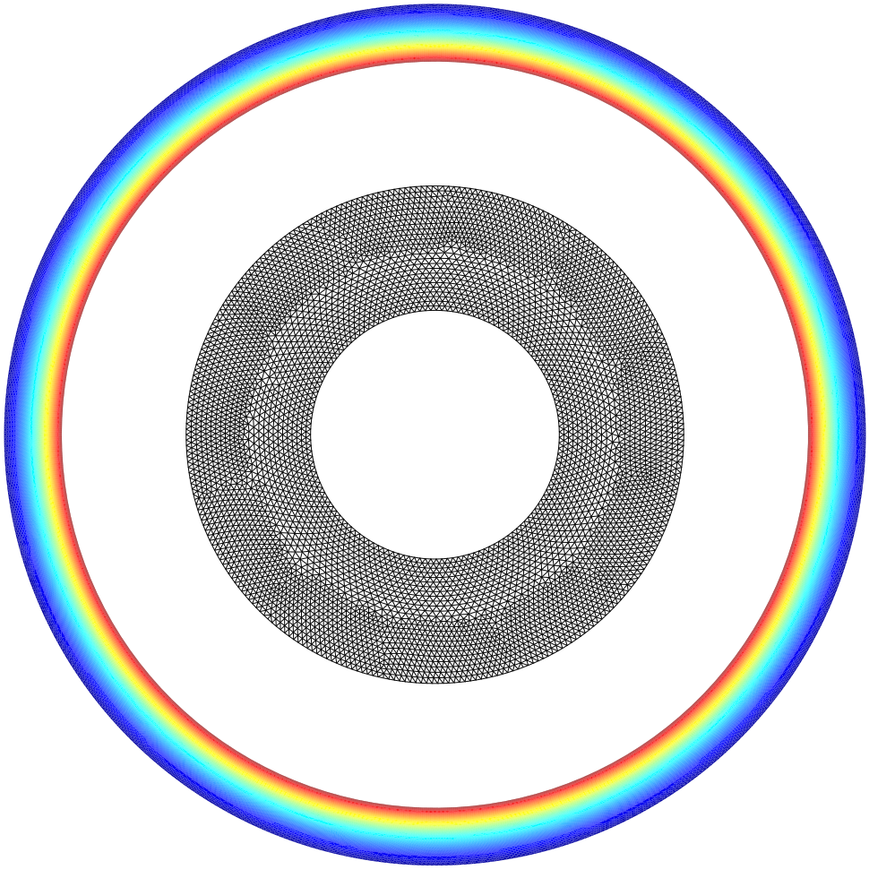
(a) Reference and deformed configuration

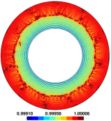
(b) Discrete Jacobian on the reference configuration

Figure 2: Quasi-incompressible annulus with $\lambda=1666.44$: sHHO(1) solution on a mesh composed of 10161 triangles.

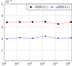
(a) Displacement error

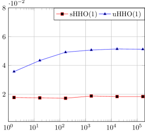
(b) Gradient error

Figure 3: Quasi-incompressible annulus: errors vs. $\lambda$ for $h=\text{2.52e-2}$

Mesh	sHHO(1)				uHHO(1)
size	Displacement		Gradient		Displacement		Gradient
$h$	Error	Order	Error	Order	Error	Order	Error	Order
1.15e-1	5.98e-2	-	3.22e-1	-	4.00e-2	-	1.23e-1	-
5.77e-2	1.81e-2	1.72	8.23e-1	1.97	1.32e-2	1.62	1.01e-1	0.28
3.45e-2	6.30e-3	2.05	3.15e-2	1.86	3.80e-3	2.42	6.60e-2	0.83
2.52e-2	3.42e-3	1.95	1.83e-2	1.73	2.03e-3	2.05	5.11e-2	0.94
1.64e-2	1.49e-3	1.93	7.98e-3	1.93	9.76e-4	1.72	3.09e-2	1.08

Table 4: Quasi-incompressible annulus: errors vs. $h$ for $k=1$ and $\lambda=1666.44$.

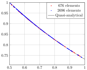
(a) sHHO(1): $u_{r}$ vs. $r$

(b) uHHO(1): $u_{r}$ vs. $r$

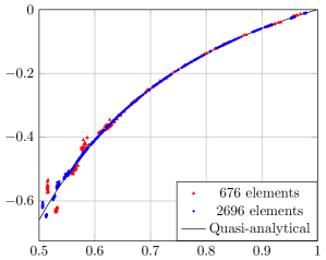
(c) sHHO(1): $P_{rr}$ vs. $r$

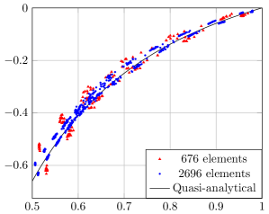
(d) uHHO(1): $P_{rr}$ vs. $r$

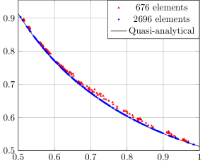
(e) sHHO(1): $P_{\theta\theta}$ vs. $r$

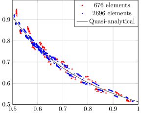
(f) uHHO(1): $P_{\theta\theta}$ vs. $r$

Figure 4: Quasi-incompressible annulus with $\lambda=1666.44$: comparison of the reference and computed values of $u_{r}$, $P_{rr}$ and $P_{\theta\theta}$ at the barycenter of the mesh cells (located in the upper quadrant) for two different meshes obtained with the sHHO and uHHO methods.

4.3 Efficiency

In this section, we compare the performance of sHHO, uHHO and that of a continuous Galerkin (cG) method in terms of efficiency when solving the three-dimensional manufactured solution from Section 4.1. The number of unknowns is the number of degrees of freedom attached to faces after static condensation for sHHO and uHHO and the number of degrees of freedom attached to nodes for cG. The cG method is based on a primal formulation realized within the industrial open-source FEM software code_aster [24] interfaced with the open-source mfront code generator [27] to generate Neohookean laws.

We present the displacement error versus the number of degrees of freedom in Fig. 5a and versus the number of non-zero entries in the stiffness matrix in Fig. 5b. Owing to the static condensation, we observe that, for the same approximation order and the same number of degrees of freedom or non-zero entries in the stiffness matrix, the displacement error is smaller for sHHO than for cG and comparable between uHHO and cG.

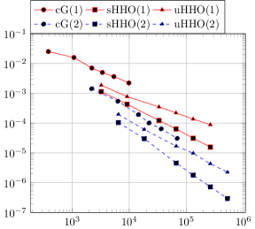
(a) Displacement error vs. number of degrees of freedom

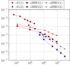
(b) Displacement error vs number of non-zero entries in the stiffness matrix

Figure 5: 3D manufactured solution: comparison of the displacement error obtained with sHHO, uHHO, and cG.

Let us now compare the time spent to solve the non-linear problem when using sHHO($k$) and uHHO($k$) with $k\in\{1,2\}$. For the present test case, the nonlinear problem is solved, for both methods, in four Newton’s iterations. The codes are instrumented to measure the assembly time $\tau_{ass}$ to build the local contributions to the global stiffness matrix and the solver time $\tau_{sol}$ which corresponds to solving the global linear system ($\tau_{ass}$ and $\tau_{sol}$ are computed after summation over all the Newton’s steps). In DiSk++, the linear algebra operations are realized using the Eigen library and the global linear system (involving face unknowns only) is solved with PardisoLU. The tests are run sequentially on a 3.4 Ghz Intel Xeon processor with 16 Gb of RAM. In Fig. 6a we plot the ratio $\tau_{\rm ass}/\tau_{\rm sol}$ versus the number of mesh faces, card$(\mathcal{F}_{h})$. We can see that on the finer meshes, the cost of local computations becomes negligible compared to that of the linear solver; we notice that the situation is a bit less favorable than for the results on linear elasticity reported in [17] since the space to reconstruct the gradient is now larger. In Fig. 6b we provide a more detailed assessment of the cost on a fixed mesh with 31621 faces. More precisely, the time $\tau_{\rm ass}$ spent in assembling the problem is now divided into two parts, one part, denoted Gradrec, to reconstruct the gradient and build the global system to solve (the part related to static condensation is not included and takes a marginal fraction of the cost), and another part, denoted Stabilization, to build the stabilization operator for the sHHO method (including the time to build the displacement reconstruction, see (23)). In addition, the time $\tau_{\rm sol}$ spent in solving the system is now denoted Solver. We observe that the difference between sHHO($k$) and uHHO($k$) is not really important; in fact, the time that uHHO($k$) spends in reconstructing the gradient in a larger space is more or less equivalent to the time that sHHO($k$) spends in building the stabilization operator. Moreover, if memory is not a limiting factor, the gradient and the stabilization can be computed once and for all, and re-used at each Newton’s step.

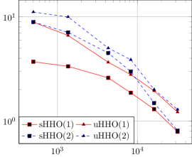
(a) $\tau_{\rm ass}$ / $\tau_{\rm sol}$ vs. card($\mathcal{F}_{h}$)

(b) Time for the different operations normalized by the total time for sHHO(1) for a mesh with 31621 faces

Figure 6: Comparison of CPU times for the sHHO and uHHO methods.

Another interesting observation is that the condition number of the global stiffness matrix for both methods is improved by static condensation, as shown in Fig. 7a where the ratio of the condition number without and with static condensation is displayed as a function of the number of face degrees of freedom. This positive effect is even increased as the mesh is refined, and it is also more pronounced when the polynomial degree $k$ is higher. Finally, we assess the influence of the stabilization parameter $\beta$ on the condition number of the stiffness matrix for sHHO($k$) $k\in\{1,2\}$. Fig. 7b reports the condition number for $\beta\in\{10^{3},10^{6}\}$ normalized by the condition number for $\beta=1$, as a function of the total number of face degrees of freedom. We observe that the condition number is amplified by a factor of $10^{2}$ when $\beta$ goes from 1 to $10^{3}$ and by a factor $10^{3}$ when $\beta$ goes from $10^{3}$ to $10^{6}$, independently of the polynomial degree $k$.

(a) Ratio of the condition number without and with static condensation vs. card($\mathcal{F}_{h}$)

(b) Condition number normalized by that for sHHO(1) or sHHO(2) with $\beta=1$ vs. card($\mathcal{F}_{h}$)

Figure 7: Condition number of the global stiffness matrix.

5 Application-driven three-dimensional examples

The goal of this section is to show that sHHO and uHHO are capable of dealing with challenging three-dimensional examples with finite deformations. For the first test case, we compare our results to those obtained with a cG method implemented in the industrial software code_aster. For the second and third test cases, we compare our results with the HDG solutions reported in [29]. In all cases, we choose $\Theta(J)=\ln J$.

5.1 Quasi-incompressible indented block

In this example, we model an indentation problem as a prototype for a contact problem. We consider the unit cube $(-1,1)\times(-1,1)\times(-1,1)$. To model the rigid indentor, the bottom surface is clamped, a vertical displacement of $-0.8$ is imposed on the subset $(-0.5,0.5)\times(-0.5,0.5)\times\{1\}$ of the top surface, and the other parts of the boundary are traction-free. We set $\mu=1$ and $\lambda=4999$ in the quasi-incompressible regime (which corresponds to a Poisson ratio of $\nu\simeq 0.4999$). The stabilization parameter needs to be taken of the order of $\beta_{0}=100$ for sHHO. Fig. 8c and Fig. 8d present the Euclidean displacement norm on the deformed configuration obtained with cG(1) and sHHO(1) respectively (the uHHO(1) solution is very close to the sHHO(1) solution). We observe the locking phenomenon affecting the cG solution. To better appreciate the influence of the parameter $\lambda$ on the discrete solutions, we plot in Fig. 8a and Fig. 8b the Euclidean displacement norm on the deformed configuration in the compressible regime ($\lambda=1$, which corresponds to a Poisson ratio of $\nu=0.25$). We observe that in the compressible regime, the results produced by the various numerical methods are all very close, whereas the cG solutions depart from the the sHHO and uHHO solutions in the quasi-incompressible regime. Finally, the computed vertical component of the discrete traction integrated over the indented top surface is plotted in Fig. 9 for sHHO and uHHO as a function of the imposed vertical displacement. The two HHO methods produce very similar results and capture well the nonlinear response of the block.

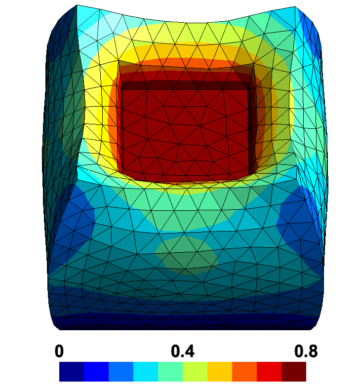
(a) Euclidean displacement norm for cG(1) in the compressible regime

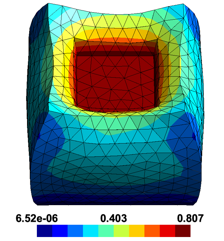
(b) Euclidean displacement norm for sHHO(1) in the compressible regime

(c) Euclidean displacement norm for cG(1) in the quasi-incompressible regime

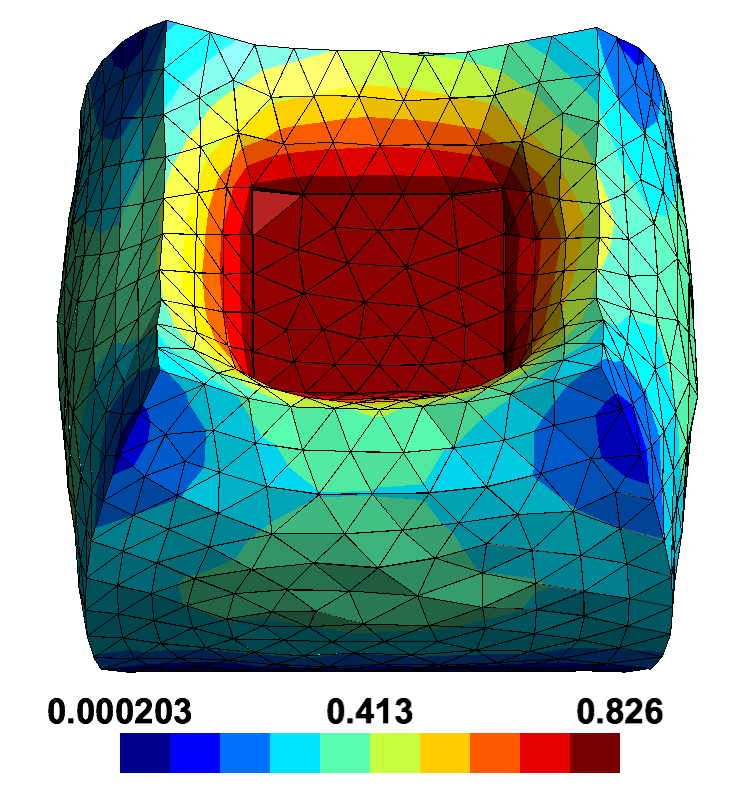
(d) Euclidean displacement norm for sHHO(1) in the quasi-incompressible regime

Figure 8: Indented block: compressible (top) and quasi-incompressible regime (bottom) with Euclidean displacement norm shown in color on a mesh composed of 5526 tetrahedra.

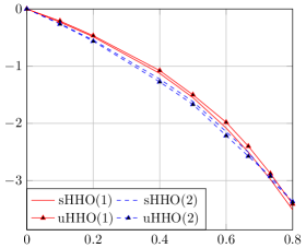
(a) Compressible block

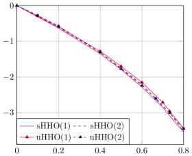
(b) Quasi-incompressible block

Figure 9: Indented block: vertical component of the computed discrete traction integrated over the indented surface versus the imposed vertical displacement using the sHHO and uHHO methods.

5.2 Cylinder under compression and shear

This test case, proposed in [29], simulates a hollow cylinder under important compression and shear (it can be seen as a controlled buckling). The cylinder in its reference configuration has a inner and outer radius of 0.75 and 1, and a height of 4. The bottom face is clamped, whereas the top face has an horizontally and vertically imposed displacement of $-1$ in both directions, and the lateral faces are traction-free. We set $\mu=0.1$, $\lambda=1$ (which corresponds to a Poisson ratio of $\nu\simeq 0.455$). For sHHO, the stabilization parameter has to be taken of the order of $\beta_{0}=100$. We notice that both sHHO and uHHO are robust and produce very close results, which compare very well with the results reported in [29]. The loading is applied in 30 steps for uHHO and in 37 steps for sHHO, leading respectively to a total of 152 and 187 Newton’s iterations. This indicates that uHHO is up to 20% more effective for this test case. Some snapshots of the solution obtained with uHHO(1) on a mesh composed of 20382 tetrahedra are shown in Fig. 10 where the color indicates the Euclidean norm of the displacement. Fig. 11 displays the von Mises stress at different loading steps on the deformed configuration. This figure allows one to observe the emerging localization of the deformation field. Finally, the evolution during the loading of the vertical component of the discrete traction integrated over the top face of the cylinder is plotted in Fig. 12. The minimum is reached when the cylinder begins to bend at $75\%$ of the loading; beyond this value, the cylinder becomes less rigid.

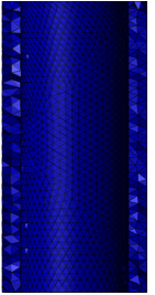
(a)

(b)

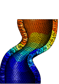
(c)

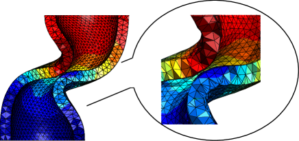
(d)

Figure 10: Sheared cylinder: snapshots of the Euclidean displacement norm on the deformed configuration at $0\%$, $40\%$, $80\%$, and $100\%$ of loading, and a zoom where the deformations are the most important (uHHO(1) solution). The color scale goes from $0.0$ (blue) to $1.8$ (red).

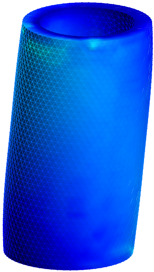
(a)

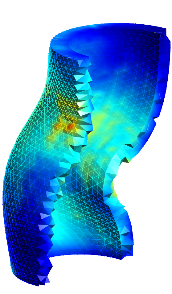
(b)

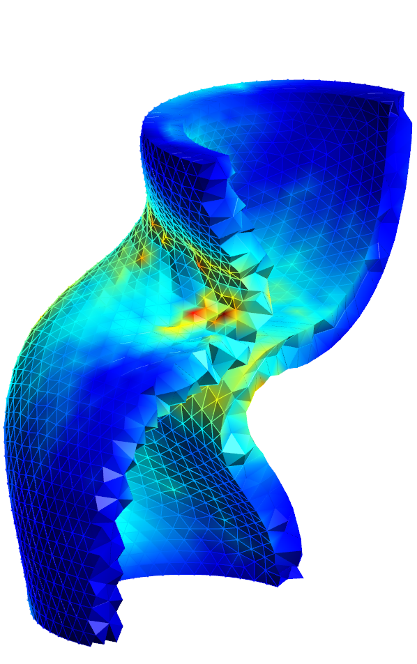
(c)

Figure 11: Sheared cylinder: von Mises stress on the deformed configuration at $40\%$, $80\%$ and $100\%$ of loading (uHHO(1) solution). The color scales goes from 0.0 (blue) to 0.275 (red).

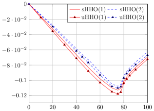
Figure 12: Sheared cylinder: evolution during the loading of the vertical component of the discrete traction integrated over the top of the cylinder for sHHO and uHHO.

5.3 Sphere with cavitating voids

The last example simulates the problem of cavitation encountered for instance in elastomers, that is, the growth of cavities under large tensile stresses [2]. Simulations of cavitation phenomena present difficulties because the growth induces significant deformations near the cavities. For a review, we refer the reader to [45]. Some conforming [33], non-conforming [45], and HDG [29] methods have already been studied for this problem. For cavitation to take place, the strain energy density has to be changed, and we consider here, as in [29], the following modified Neohookean law:

$$\Psi(\underline{\underline{\boldsymbol{F}}})=\frac{2\mu}{3^{5/4}}\left(\underline{\underline{\boldsymbol{F}}}:\underline{\underline{\boldsymbol{F}}}\right)^{3/4}-\mu\ln J+\frac{\lambda}{2}(\ln J)^{2},$$ (38)

where $\mu$ and $\lambda$ are constant parameters. We set $\mu=1$, $\lambda=1$ (which corresponds to a Poisson ratio of $\nu=0.25$).

The reference configuration consists of a unit sphere of radius 1 with two spherical cavities. The origin of the Cartesian coordinate system is the center of the sphere. The first cavity has a radius of 0.15 and its center is the point of coordinates $(-0.7,-0.7,0)$, and the second cavity has a radius of 0.2 and its center is the point of coordinates $(0.25,0.25,0.25)$. A displacement $\underline{\boldsymbol{u}}(\underline{\boldsymbol{X}})=r\underline{\boldsymbol{X}}$ with $r\geq 0$ is imposed on the outer surface ($|\underline{\boldsymbol{X}}|=1$) of the sphere. The stabilization parameter has to be taken of the order of $\beta_{0}=100$ for sHHO. The mesh is composed of $32288$ tetrahedra, and the value of $r$ is increased progressively until the moment where the Newton’s method fails to converge. Some snapshots of the Euclidean displacement norm are shown in Fig. 13 on the deformed configuration for uHHO(2). We also present a zoom near the region where the two cavities are only separated by a thin layer. The reported solution compares very well with the HDG solution from [29]. Interestingly, the maximum value attained of $r$ is larger for uHHO than for sHHO and is larger for $k=2$ than for $k=1$ (see Fig. 14). For $k=2$, the maximum value of $r$ is 2.52 for uHHO and 2.13 for sHHO, which indicates about 15% more robustness for uHHO than for sHHO to handle extreme loading situations in this case. Finally, Fig. 14 presents the radial component of the discrete traction integrated over the outer surface of the sphere versus the imposed radial displacement obtained with sHHO and uHHO.

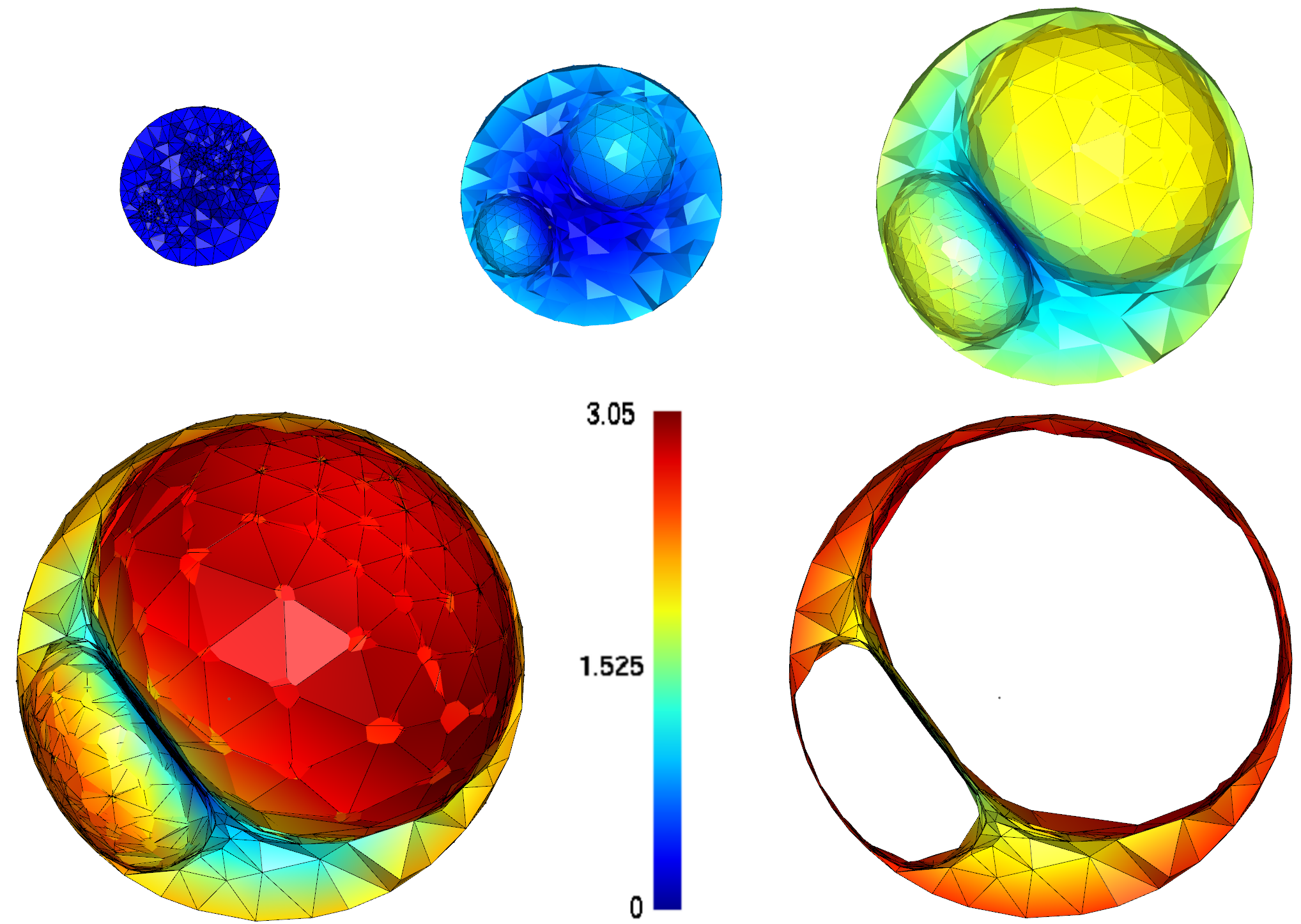
Figure 13: Sphere with cavitating voids: snaphots of the Euclidean displacement norm at $r=0$, $r=0.8$, $r=1.6$ and $r=2.52$ of loading (the sphere is cut along the Equatorial plane) for uHHO(2) on the deformed configuration. The bottom right plot shows a thin slice of the sphere (still along the Equatorial plane) for $r=2.52$.

(a)

(b)

Figure 14: Sphere with cavitating voids: radial component of the discrete traction integrated over the outer surface versus the imposed radial displacement obtained with sHHO (left) and uHHO (right). Notice in both cases the larger value attained by $r$ for $k=2$.

6 Conclusion

We have proposed and evaluated numerically two HHO methods to approximate hyperelastic materials undergoing finite deformations. Both methods deliver solutions that compare well to the existing literature on challenging three-dimensional test cases, such as a hollow cylinder under compression and shear or a sphere under traction with two cavitating voids. In addition, both methods remain well-behaved in the quasi-incompressible limit, as observed numerically on an annulus under traction and on the indentation of a rectangular block. The test cases with analytical solution also show that both methods are competitive with respect to an industrial software using conforming finite elements. The stabilized HHO method rests on a firmer theoretical basis than the unstabilized method, but requires the introduction and tuning of a stabilization parameter that can become fairly large in the quasi-incompressible limit. The unstabilized HHO method avoids any stabilization by introducing a stable gradient reconstructed in the higher-order polynomial space ${\mathbb{P}}_{d}^{k+1}(T;{\mathbb{R}}^{d\times d})$, but for smooth solutions, the convergence rate is one order lower than with the stabilized method, i.e., the unstabilized method still converges, but in a suboptimal way. For compressible materials, the unstabilized method appears to be somewhat more competitive than the stabilized method since it requires less Newton’s iterations and, at the same time, supports stronger loads, as observed in particular in the case of cavitating voids in the sphere.

We have also evaluated numerically the unstabilized HHO method using Raviart–Thomas–Nédélec reconstructions of the gradient (detailed results were not reported herein for brevity). We have retrieved the optimal-order convergence rates for smooth solutions, but the method seems to be somewhat less robust for strongly nonlinear problems. For example, in the case of the sphere with cavitating voids for $k=1$, if the discrete gradient is reconstructed in $\mathbb{RTN}_{d}^{k}(T;{\mathbb{R}}^{d\times d})$, then the maximum value is $r=1.12$ whereas, if the discrete gradient is reconstructed in $\mathbb{RTN}_{d}^{k+1}(T;{\mathbb{R}}^{d\times d})$ (which contains the space ${\mathbb{P}}_{d}^{k+1}(T;{\mathbb{R}}^{d\times d})$), then the maximum value for $r$ is the same as for uHHO using ${\mathbb{P}}_{d}^{k+1}(T;{\mathbb{R}}^{d\times d})$ and $k=1$ ($r=1.92$).

Among possible perspectives of this work, we mention the devising of a reconstruction based on the ideas introduced in [25] for dG methods, and the use of different reconstructions for the isochoric and volumic parts of the energy density. The present methods can also be applied to approximate other nonlinear problems. For instance, elasto-plasticity constitutes the subject of ongoing work.

References

• [1] J. M. Ball. Convexity conditions and existence theorems in nonlinear elasticity. Arch. Rational Mech. Anal., 63(4):337–403, 1976/77.
• [2] J. M. Ball. Discontinuous equilibrium solutions and cavitation in nonlinear elasticity. Philos. Trans. Roy. Soc. London Ser. A, 306(1496):557–611, 1982.
• [3] L. Beirão da Veiga, C. Lovadina, and D. Mora. A virtual element method for elastic and inelastic problems on polytope meshes. Comput. Methods Appl. Mech. Engrg., 295:327–346, 2015.
• [4] D. Boffi, M. Botti, and D. A. Di Pietro. A nonconforming high-order method for the Biot problem on general meshes. SIAM J. Sci. Comput., 38(3):A1508–A1537, 2016.
• [5] J. Bonet and R. D. Wood. Nonlinear continuum mechanics for finite element analysis. Cambridge university press, Cambridge, 1997.
• [6] M. Botti, D. A. Di Pietro, and P. Sochala. A Hybrid High-Order Method for Nonlinear Elasticity. SIAM J. Numer. Anal., 55(6):2687–2717, 2017.
• [7] C. Carstensen and F. Hellwig. Low-order discontinuous Petrov-Galerkin finite element methods for linear elasticity. SIAM J. Numer. Anal., 54(6):3388–3410, 2016.
• [8] H. Chi, L. Beirão da Veiga, and G. H. Paulino. Some basic formulations of the virtual element method (VEM) for finite deformations. Comput. Methods Appl. Mech. Engrg., 318:148–192, 2017.
• [9] P. G. Ciarlet. Mathematical elasticity. Vol. I, volume 20 of Studies in Mathematics and its Applications. North-Holland Publishing Co., Amsterdam, 1988. Three-dimensional elasticity.
• [10] M. Cicuttin, D. D. Pietro, and A. Ern. Implementation of Discontinuous Skeletal methods on arbitrary-dimensional, polytopal meshes using generic programming. J. Comput. Appl. Math., 2017. published online http://dx.doi.org/10.1016/j.cam.2017.09.017.
• [11] B. Cockburn, D. A. Di Pietro, and A. Ern. Bridging the hybrid high-order and hybridizable discontinuous Galerkin methods. ESAIM Math. Model. Numer. Anal., 50(3):635–650, 2016.
• [12] B. Cockburn, J. Gopalakrishnan, and R. Lazarov. Unified hybridization of discontinuous Galerkin, mixed, and continuous Galerkin methods for second order elliptic problems. SIAM J. Numer. Anal., 47(2):1319–1365, 2009.
• [13] B. Cockburn, J. Gopalakrishnan, N. C. Nguyen, J. Peraire, and F.-J. Sayas. Analysis of HDG methods for Stokes flow. Math. Comp., 80(274):723–760, 2011.
• [14] B. Cockburn, D. Schötzau, and J. Wang. Discontinuous Galerkin methods for incompressible elastic materials. Comput. Methods Appl. Mech. Engrg., 195(25-28):3184–3204, 2006.
• [15] D. A. Di Pietro, J. Droniou, and A. Ern. A discontinuous-skeletal method for advection-diffusion-reaction on general meshes. SIAM J. Numer. Anal., 53(5):2135–2157, 2015.
• [16] D. A. Di Pietro, J. Droniou, and G. Manzini. Discontinuous Skeletal Gradient Discretisation Methods on polytopal meshes. accepted for publication, https://hal.archives-ouvertes.fr/hal-01564598, 2017.
• [17] D. A. Di Pietro and A. Ern. A hybrid high-order locking-free method for linear elasticity on general meshes. Comput. Methods Appl. Mech. Engrg., 283:1–21, 2015.
• [18] D. A. Di Pietro, A. Ern, and S. Lemaire. An arbitrary-order and compact-stencil discretization of diffusion on general meshes based on local reconstruction operators. Comput. Methods Appl. Math., 14(4):461–472, 2014.
• [19] D. A. Di Pietro, A. Ern, and S. Lemaire. A review of hybrid high-order methods: formulations, computational aspects, comparison with other methods. In Building bridges: connections and challenges in modern approaches to numerical partial differential equations, volume 114 of Lect. Notes Comput. Sci. Eng., pages 205–236. Springer, [Cham], 2016.
• [20] D. A. Di Pietro, A. Ern, A. Linke, and F. Schieweck. A discontinuous skeletal method for the viscosity-dependent Stokes problem. Comput. Methods Appl. Mech. Engrg., 306:175–195, 2016.
• [21] D. A. Di Pietro and S. Krell. A Hybrid High-Order method for the steady incompressible Navier–Stokes problem. J. Sci. Comput., 2017. published online https://doi.org/10.1007/s10915-017-0512-x.
• [22] J. Droniou and B. P. Lamichhane. Gradient schemes for linear and non-linear elasticity equations. Numer. Math., 129(2):251–277, 2015.
• [23] D. A. Dunavant. High degree efficient symmetrical Gaussian quadrature rules for the triangle. Internat. J. Numer. Methods Engrg., 21(6):1129–1148, 1985.
• [24] Electricité de France. Finite element $\bf\it code\_aster$, structures and thermomechanics analysis for studies and research. Open source on www.code-aster.org, 1989–2017.
• [25] R. Eymard and C. Guichard. The discontinuous Galerkin gradient discretisation. Preprint hal-01535147, June 2017.
• [26] P. Hansbo and M. G. Larson. Discontinuous Galerkin methods for incompressible and nearly incompressible elasticity by Nitsche’s method. Comput. Methods Appl. Mech. Engrg., 191(17-18):1895–1908, 2002.
• [27] T. Helfer, B. Michel, J.-M. Proix, M. Salvo, J. Sercombe, and M. Casella. Introducing the open-source mfront code generator: Application to mechanical behaviours and material knowledge management within the PLEIADES fuel element modelling platform. Comput. Math. Appl., 70(5):994–1023, 2015.
• [28] L. John, M. Neilan, and I. Smears. Stable discontinuous galerkin fem without penalty parameters. In B. Karasözen, M. Manguoğlu, M. Tezer-Sezgin, S. Göktepe, and Ö. Uğur, editors, Numerical Mathematics and Advanced Applications ENUMATH 2015, pages 165–173. Springer International Publishing, 2016.
• [29] H. Kabaria, A. J. Lew, and B. Cockburn. A hybridizable discontinuous Galerkin formulation for non-linear elasticity. Comput. Methods Appl. Mech. Engrg., 283:303–329, 2015.
• [30] J. Krämer, C. Wieners, B. Wohlmuth, and L. Wunderlich. A hybrid weakly nonconforming discretization for linear elasticity. Proc. Appl. Math. Mech., 16(1):849–850, 2016.
• [31] C. Lehrenfeld. Hybrid Discontinuous Galerkin methods for solving incompressible flow problems. PhD thesis, Rheinisch-Westfälischen Technischen Hochschule Aachen, 2010.
• [32] A. Lew, P. Neff, D. Sulsky, and M. Ortiz. Optimal BV estimates for a discontinuous Galerkin method for linear elasticity. AMRX Appl. Math. Res. Express, 2004(3):73–106, 2004.
• [33] Y. Lian and Z. Li. A numerical study on cavitation in nonlinear elasticity—defects and configurational forces. Math. Models Methods Appl. Sci., 21(12):2551–2574, 2011.
• [34] N. C. Nguyen and J. Peraire. Hybridizable discontinuous Galerkin methods for partial differential equations in continuum mechanics. J. Comput. Phys., 231(18):5955–5988, 2012.
• [35] L. Noels and R. Radovitzky. A general discontinuous Galerkin method for finite hyperelasticity. Formulation and numerical applications. Internat. J. Numer. Methods Engrg., 68(1):64–97, 2006.
• [36] R. W. Ogden. Non-linear elastic deformations. Dover Publication, New-York, 1997.
• [37] S.-C. Soon. Hybridizable Discontinuous Galerkin Method for Solid Mechanics. PhD thesis, University of Minnesota, 2008.
• [38] S.-C. Soon, B. Cockburn, and H. K. Stolarski. A hybridizable discontinuous Galerkin method for linear elasticity. Internat. J. Numer. Methods Engrg., 80(8):1058–1092, 2009.
• [39] A. ten Eyck, F. Celiker, and A. Lew. Adaptive stabilization of discontinuous Galerkin methods for nonlinear elasticity: analytical estimates. Comput. Methods Appl. Mech. Engrg., 197(33-40):2989–3000, 2008.
• [40] A. ten Eyck, F. Celiker, and A. Lew. Adaptive stabilization of discontinuous Galerkin methods for nonlinear elasticity: motivation, formulation, and numerical examples. Comput. Methods Appl. Mech. Engrg., 197(45-48):3605–3622, 2008.
• [41] A. ten Eyck and A. Lew. Discontinuous Galerkin methods for non-linear elasticity. Internat. J. Numer. Methods Engrg., 67(9):1204–1243, 2006.
• [42] C. Wang, J. Wang, R. Wang, and R. Zhang. A locking-free weak Galerkin finite element method for elasticity problems in the primal formulation. J. Comput. Appl. Math., 307:346–366, 2016.
• [43] P. Wriggers, B. D. Reddy, W. Rust, and B. Hudobivnik. Efficient virtual element formulations for compressible and incompressible finite deformations. Comput. Mech., 58, 2017.
• [44] S. Wulfinghoff, H. R. Bayat, A. Alipour, and S. Reese. A low-order locking-free hybrid discontinuous Galerkin element formulation for large deformations. Comput. Methods Appl. Mech. Engrg., 323:353–372, 2017.
• [45] X. Xu and D. Henao. An efficient numerical method for cavitation in nonlinear elasticity. Math. Models Methods Appl. Sci., 21(8):1733–1760, 2011.