FO model checking of geometric graphs

Abstract

Over the past two decades the main focus of research into first-order (FO) model checking algorithms has been on sparse relational structures – culminating in the FPT algorithm by Grohe, Kreutzer and Siebertz for FO model checking of nowhere dense classes of graphs. On contrary to that, except the case of locally bounded clique-width only little is currently known about FO model checking of dense classes of graphs or other structures. We study the FO model checking problem for dense graph classes definable by geometric means (intersection and visibility graphs). We obtain new nontrivial FPT results, e.g., for restricted subclasses of circular-arc, circle, box, disk, and polygon-visibility graphs. These results use the FPT algorithm by Gajarský et al. for FO model checking of posets of bounded width. We also complement the tractability results by related hardness reductions.

Keywords: first-order logic; model checking; fixed-parameter tractability; intersection graphs; visibility graphs

1 Introduction

Algorithmic meta-theorems are results stating that all problems expressible in a certain language are efficiently solvable on certain classes of structures, e.g. of finite graphs. Note that the model checking problem for first-order logic – given a graph $G$ and an FO formula $\phi$, we want to decide whether $G$ satisfies $\phi$ (written as $G\models\phi$) – is trivially solvable in time $|V(G)|^{\mathcal{O}(|\phi|)}$. “Efficient solvability” hence in this context often means fixed-parameter tractability (FPT); that is, solvability in time $f(|\phi|)\cdot|V(G)|^{\mathcal{O}(1)}$ for some computable function $f$.

In the past two decades algorithmic meta-theorems for FO logic on sparse graph classes received considerable attention. While the algorithm of [5] for MSO on graphs of bounded clique-width implies fixed-parameter tractability of FO model checking on graphs of locally bounded clique-width via Gaifman’s locality, one could go far beyond that. After the result of Seese [29] proving fixed-parameter tractability of FO model checking on graphs of bounded degree there followed a series of results [14, 6, 10] establishing the same conclusion for increasingly rich sparse graph classes. This line of research culminated in the result of Grohe, Kreutzer and Siebertz [22], who proved that FO model checking is FPT on nowhere dense graph classes.

While the result of [22] is the best possible in the following sense—if a graph class ${\cal D}$ is monotone (closed on taking subgraphs) and not nowhere dense, then the FO model checking problem on ${\cal D}$ is as hard as that on all graphs; this does not exclude interesting FPT meta-theorems on somewhere dense non-monotone graph classes. Probably the first extensive work of the latter dense kind, beyond locally bounded clique-width, was that of Ganian et al. [18] studying subclasses of interval graphs in which FO model checking is FPT (precisely, those which use only a finite set of interval lengths). Another approach has been taken in the works of Bova, Ganian and Szeider [3] and Gajarský et al. [15], which studied FO model checking on posets – posets can be seen as typically quite dense special digraphs. Altogether, however, only very little is known about FO model checking of somewhere dense graph classes (except perhaps specialised [17]).

The result of Gajarský et al. [15] claims that FO model checking is FPT on posets of bounded width (size of a maximum antichain), and it happens to imply [18] in a stronger setting (see below). One remarkable message of [15] is the following (citation): The result may also be used directly towards establishing fixed-parameter tractability for FO model checking of other graph classes. Given the ease with which it ([15] ) implies the otherwise non-trivial result on interval graphs [18], it is natural to ask what other (dense) graph classes can be interpreted in posets of bounded width. Inspired by the geometric case of interval graphs, we propose to study dense graph classes defined in geometric terms, such as intersection and visibility graphs, with respect to tractability of their FO model checking problem.

The motivation for such study is a two-fold. First, intersection and visibility graphs present natural examples of non-monotone somewhere dense graph classes to which the great “sparse” FO tractability result of [22] cannot be (at least not easily) applied. Second, their supplementary geometric structure allows to better understand (as we have seen already in [18]) the boundaries of tractability of FO model checking on them, which is, to current knowledge, terra incognita for hereditary graph classes in general.

Our results mainly concern graph classes which are related to interval graphs. Namely, we prove (Theorem 3.1) that FO model checking is FPT on circular-arc graphs (these are interval graphs on a circle) if there is no long chain of arcs nested by inclusion. This directly extends the result of [18] and its aforementioned strengthening in [15] (with bounding chains of nested intervals instead of their lengths). We similarly show tractability of FO model checking of interval-overlap graphs, also known as circle graphs, of bounded independent set size (Theorem 3.3), and of restricted subclasses of box and disk graphs which naturally generalize interval graphs to two dimensions (Theorem 3.6 and 3.7).

On the other hand, for all of the studied cases we also show that whenever we relax our additional restrictions (parameters), the FO model checking problem becomes as hard on our intersection classes as on all graphs (Corollary 4.2). Some of our hardness claims hold also for the weaker $\exists$FO model checking problem (Proposition 4.4).

Another well studied dense graph class in computational geometry are visibility graphs of polygons, which have been largely explored in the context of recognition, partition, guarding and other optimization problems [19, 28]. We consider some established special cases, involving weak visibility, terrain and fan polygons. We prove that FO model checking is FPT for the visibility graphs of a weak visibility polygon of a convex edge, with bounded number of reflex (non-convex) vertices (Theorem 5.4). On the other hand, without bounding reflex vertices, FO model checking remains hard even for the much more special case of polygons that are terrain and convex fans at the same time (Theorem 5.1).

As noted above, our fixed-parameter tractability proofs use the strong result [15] on FO model checking of posets of bounded width. We refer to Section 2 for a detailed explanation of the technical terms used here. Briefly, for a given graph $G$ from the respective class and a formula $\phi$, we show how to efficiently construct a poset ${\cal P}_{G}$ of bounded width and a related FO formula $\phi^{I}$ such that $G\models\phi$ iff ${\cal P}_{G}\models\phi^{I}$, and then solve the latter problem. In constructing the poset ${\cal P}_{G}$ we closely exploit the respective geometric representation of $G$.

With respect to the previously known results, we remark that our graph classes are not sparse, as they all contain large complete or complete bipartite subgraphs. For many of them, namely unit circular-arc graphs, circle graphs of bounded independence number, and unit box and disk graphs, we can also show that they are of locally unbounded clique-width by a straightforward adaptation of an argument from [18] (Proposition 3.10). For the visibility graphs of a weak visibility polygon of a convex edge, we leave the question of bounding their local clique-width open.

Lastly, we particularly emphasize the seemingly simple tractable case (Corollary 3.4) of permutation graphs of bounded clique size: in relation to so-called stability notion (cf. [1]), already the hereditary class of triangle-free permutation graphs has the $n$-order property (i.e., is not stable), and yet FO model checking of this class is FPT. This example presents a natural hereditary and non-stable graph class with FPT FO model checking other than, say, graphs of bounded clique-width. We suggest that if we could fully understand the precise breaking point(s) of FP tractability of FO model checking on simply described intersection classes like the permutation graphs, then we would get much better insight into FP tractability of FO model checking of general hereditary graph classes.

2 Preliminaries

We recall some established concepts concerning intersection graphs and first-order logic.

Graphs and intersection graphs.

We work with finite simple undirected graphs and use standard graph theoretic notation. We refer to the vertex set of a graph $G$ as to $V(G)$ and to its edge set as to $E(G)$, and we write shortly $uv$ for an edge $\{u,v\}$. As it is common in the context of FO logic on graphs, vertices of our graphs can carry arbitrary labels.

Considering a family of sets ${\mathcal{S}}$ (in our case, of geometric objects in the plane), the intersection graph of ${\mathcal{S}}$ is the simple graph $G$ defined by $V(G):={\mathcal{S}}$ and $E(G):=\{AB:A,B\in{\mathcal{S}},\,A\cap B\not=\emptyset\}$. In respect of algorithmic questions, it is important to distinguish whether an intersection graph $G$ is given on the input as an abstract graph $G$, or alongside with its intersection representation ${\mathcal{S}}$. Usually, finding an appropriate representation for given $G$ is a hard task, but we will mostly restrict our attention to intersection classes for which there exists a polynomial-time algorithm for computing the representation.

One folklore example of a widely studied intersection graph class are interval graphs – the intersection graphs of intervals on the real line. Interval graphs enjoy many nice algorithmic properties, e.g., their representation can be constructed quickly, and generally hard problems like clique, independent set and chromatic number are solvable in polynomial time for them.

For a general overview and extensive reference guide of intersection graph classes we suggest to consult the online system ISGCI [7]. Regarding visibility graphs, which present a kind of geometric graphs behaving very differently from intersection graphs, we refer to Section 5 for their separate more detailed treatment.

FO logic.

The first-order logic of graphs (abbreviated as FO) applies the standard language of first-order logic to a graph $G$ viewed as a relational structure with the domain $V(G)$ and the single binary (symmetric) relation $E(G)$. That is, in graph FO we have got the standard predicate $x=y$, a binary predicate $edge(x,y)$ with the usual meaning $xy\in E(G)$, an arbitrary number of unary predicates $L(x)$ with the meaning that $x$ holds the label $L$, usual logical connectives $\wedge,\vee,\to$, and quantifiers $\forall x$, $\exists x$ over the vertex set $V(G)$.

For example, $\phi(x,y)\equiv\exists z\big{(}edge(x,z)\wedge edge(y,z)\wedge red(z)\big{)}$ states that the vertices $x,y$ have a common neighbour in $G$ which has got label ‘red’. One can straightforwardly express in FO properties such as $k$-clique $\exists x_{1},\dots,x_{k}\big{(}\bigwedge_{i<j=1}^{k}(edge(x_{i},x_{j})\wedge x_{i}\not=x_{j})\big{)}$ and $k$-dominating set $\exists x_{1},\dots,x_{k}\forall y\big{(}\bigvee_{i=1}^{k}(edge(x_{i},y)\vee y=x_{i})\big{)}$. Specially, an FO formula $\phi$ is existential (abbreviated as $\exists$FO) if it can be written as $\phi\equiv\exists x_{1},\dots,x_{k}\,\psi$ where $\psi$ is quantifier-free. For example, $k$-clique is $\exists$FO while $k$-dominating set is not.

Likewise, FO logic of posets treats a poset ${\cal P}=(P,\sqsubseteq)$ as a finite relational structure with the domain $P$ and the (antisymmetric) binary predicate $x\sqsubseteq y$ (instead of the predicate $edge$) with the usual meaning. Again, posets can be arbitrarily labelled by unary predicates.

Parameterized model checking.

Instances of a parameterized problem can be considered as pairs $\langle I,k\rangle$ where $I$ is the main part of the instance and $k$ is the parameter of the instance; the latter is usually a non-negative integer. A parameterized problem is fixed-parameter tractable (FPT) if instances $\langle I,k\rangle$ of size $n$ can be solved in time $O(f(k)\cdot n^{c})$ where $f$ is a computable function and $c$ is a constant independent of $k$. In parameterized model checking, instances are considered in the form $\langle(G,\phi),|\phi|\rangle$ where $G$ is a structure, $\phi$ a formula, the question is whether $G\models\phi$ and the parameter is the size of $\phi$.

When speaking about the FO model checking problem in this paper, we always implicitly consider the formula $\phi$ (precisely its size) as a parameter. We shall use the following result:

Theorem 2.1 ([15]).

The FO model checking problem of (arbitrarily labelled) posets, i.e., deciding whether ${\cal P}\models\phi$ for a labelled poset ${\cal P}$ and FO $\phi$, is fixed-parameter tractable with respect to $|\phi|$ and the width of ${\cal P}$ (this is the size of the largest antichain in ${\cal P}$).

We also present, for further illustration, a result on FO model checking of interval graphs with bounded nesting. A set ${\cal A}$ of intervals (interval representation) is called proper if there is no pair of intervals in ${\cal A}$ such that one is contained in the other. We call ${\cal A}$ a $k$-fold proper set of intervals if there exists a partition ${{\cal A}}={{\cal A}}_{1}\cup\dots\cup{{\cal A}}_{k}$ such that each ${{\cal A}}_{j}$ is a proper interval set for $j=1,\dots,k$. Clearly, ${\cal A}$ is $k$-fold proper if and only if there is no chain of $k+1$ inclusion-nested intervals in ${\cal A}$. From Theorem 2.1 one can, with help of relatively easy arguments (Lemma 3.2), derive the following:

Theorem 2.2 ([15], cf. Proposition 2.4 and Lemma 3.2).

Let $G$ be an interval graph given alongside with its $k$-fold proper interval representation ${\cal A}$. Then FO model checking of $G$ is FPT with respect to the parameters $k$ and the formula size.

Parameterized hardness.

For some parameterized problems, like the $k$-clique on all graphs, we do not have nor expect any FPT algorithm. To this end, the theory of parameterized complexity of Downey and Fellows [8] defines complexity classes $W[t]$, $t\geq 1$, such that the $k$-clique problem is complete for $W[1]$ (the least class). Furthermore, theory also defines a larger complexity class $AW[*]$ containing all of $W[t]$. Problems that are $W[1]$-hard do not admit an FPT algorithm unless the established Exponential Time Hypothesis fails.

Theorem 2.3 ([9]).

The FO model checking problem (where the formula size is the parameter) of all simple graphs is $AW[*]$-complete.

Dealing with parameterized hardness of FO model checking, one should also mention the related induced subgraph isomorphism problem: for a given input graph $G$, and a graph $H$ as the parameter, decide whether $G$ has an induced subgraph isomorphic to $H$. Note that this includes the clique and independent set problems. Induced subgraph isomorphism (parameterized by the subgraph size) is clearly a weaker problem than parameterized FO model checking, since one may “guess” the subgraph with $|V(H)|$ existential quantifiers and then verify it edge by edge. Consequently, every parameterized hardness result for induced subgraph isomorphism readily implies same hardness results for $\exists$FO and FO model checking.

FO interpretations.

Interpretations are a standard tool of logic and finite model theory. To keep our paper short, we present here only a simplified description of them, tailored specifically to our need of interpreting geometric graphs in posets.

An FO interpretation is a pair $I=(\nu,\psi)$ of poset FO formulas $\nu(x)$ and $\psi(x,y)$ (of one and two free variables, respectively). For a poset ${\cal P}$, this defines a graph $G:=I({\cal P})$ such that $V(G)=\{v:{\cal P}\models\nu(v)\}$ and $E(G)=\{uv:u,v\in V(G),\,{\cal P}\models\psi(u,v)\vee\psi(v,u)\}$. Possible labels of the elements are naturally inherited from ${\cal P}$ to $G$. Moreover, for a graph FO formula $\phi$ the interpretation $I$ defines a poset FO formula $\phi^{I}$ recursively as follows: every occurrence of ${edge}(x,y)$ is replaced by $\psi(x,y)\vee\psi(y,x)$, every $\exists x\,\sigma$ is replaced by $\exists x\,(\nu(x)\wedge\sigma)$ and $\forall x\,\sigma$ by $\forall x\,(\nu(x)\to\sigma)$. Then, obviously, ${\cal P}\models\phi^{I}\Longleftrightarrow G\models\phi$.

Usefulness of the concept is illustrated by the following trivial claim:

Proposition 2.4.

Let ${\mathcal{P}}$ be a class of posets such that the FO model checking problem of ${\mathcal{P}}$ is FPT, and let ${\mathcal{G}}$ be a class of graphs. Assume there is a computable FO interpretation $I$, and for every graph $G\in{\mathcal{G}}$ we can in polynomial time compute a poset ${\cal P}\in{\mathcal{P}}$ such that $G=I({\cal P})$. Then the FO model checking problem of ${\mathcal{G}}$ is in FPT.

Proof.

Given $G\in{\mathcal{G}}$ and formula $\phi$ (the parameter), we construct $\phi^{I}$ and ${\cal P}\in{\mathcal{P}}$ such that $G=I({\cal P})$, and call the assumed algorithm to decide ${\cal P}\models\phi^{I}$. ∎

3 Tractability for Intersection Classes

3.1 Circular-arc graphs

Circular-arc graphs are intersection graphs of arcs (curved intervals) on a circle. They clearly form a superclass of interval graphs, and they enjoy similar nice algorithmic properties as interval graphs, such as efficient construction of the representation [27], and easy computation of, say, maximum independent set or clique.

Since the FO model checking problem is $AW[*]$-complete on interval graphs [18], the same holds for circular-arc graphs in general. Furthermore, by [26, 24] already $\exists$FO model checking is $W[1]$-hard for interval and circular-arc graphs. A common feature of these hardness reductions (see more discussion in Section 4) is their use of unlimited chains of nested intervals/arcs. Analogously to Theorem 2.2, we prove that considering only $k$-fold proper circular-arc representations (the definition is the same as for $k$-fold proper interval representations) makes FO model checking of circular-arc graphs tractable.

Theorem 3.1.

Let $G$ be a circular-arc graph given alongside with its $k$-fold proper circular-arc representation ${\cal A}$. Then FO model checking of $G$ is FPT with respect to the parameters $k$ and the formula size.

Note that we can (at least partially) avoid the assumption of having a representation ${\cal A}$ in the following sense. Given an input graph $G$, we compute a circular-arc representation ${\cal A}$ using [27], and then we easily determine the least $k^{\prime}$ such that ${\cal A}$ is $k^{\prime}$-fold proper. However, without further considerations, this is not guaranteed to provide the minimum $k$ over all circular-arc representations of $G$, and not even $k^{\prime}$ bounded in terms of the minimum $k$.

Our proof will be based on the following extension of the related argument from [15]:

Lemma 3.2 (parts from [15, Section 5]).

Let ${\cal B}$ be a $k$-fold proper set of intervals for some integer $k>0$, such that no two intervals of ${\cal B}$ share an endpoint. There exist formulas $\nu,\psi,\vartheta$ depending on $k$, and a labelled poset ${\cal P}$ of width $k+1$ computable in polynomial time from ${\cal B}$, such that all the following hold:

• The domain of ${\cal P}$ includes (the intervals from) ${\cal B}$, and ${\cal P}\models\nu(x)$ iff $x\in{\cal B}$,

• ${\cal P}\models\psi(x,y)$ for intervals $x,y\in{\cal B}$ iff $x\cap y\not=\emptyset$ (edge relation of the interval graph of ${\cal B}$),

• ${\cal P}\models\vartheta(x,y)$ for intervals $x,y\in{\cal B}$ iff $x\subseteq y$ (containment of intervals).

Proof.

The first part repeats an argument from [15, Section 5]. Let $D:=\{a,b:[a,b]\in{\cal B}\}$ be the set of all interval ends, and ${\cal B}={\cal B}_{1}\cup\dots\cup{\cal B}_{k}$ be such that each ${\cal B}_{j}$ is a proper interval set for $j=1,\dots,k$. Let $P:=D\cup{\cal B}$. We define a poset ${\cal P}=(P,\leq^{\cal P})$ as follows:

• for numbers $d_{1},d_{2}\in D$ it is $d_{1}\leq^{\cal P}\!d_{2}$ iff $d_{1}\leq d_{2}$,

• for $j\in\{1,\dots,k\}$ and intervals $t_{1},t_{2}\in{\cal B}_{j}$, it is $t_{1}\leq^{\cal P}\!t_{2}$ iff $t_{1}$ is not to the right of $t_{2}$,

• for every $t=[a,b]\in\cal B$ and every $d\in D$, it is $t\leq^{\cal P}\!d$ iff $d\geq b$, and $d\leq^{\cal P}\!t$ iff $d\leq a$.

An informal meaning of this definition of ${\cal P}$ is that every interval $[a,b]$ from ${\cal B}$ is larger than its left end $a$ (and hence larger than all interval ends before $a$), and the interval is smaller than its right end $b$ (and hence smaller than all interval ends after $b$). The interval $[a,b]$ is incomparable with all ends (of other intervals) which are strictly between $a$ and $b$.

Using that each ${\cal B}_{j}$ is proper, one can verify that ${\cal P}$ indeed is a poset. The set $P$ can be partitioned into $k+1$ chains; $D$ and ${\cal B}_{1},\dots,{\cal B}_{k}$. Hence the width of ${\cal P}$ is at most $k+1$.

In order to define the formulas, we give a special label ‘$D$’ to the set $D$. Then

$$\nu(x)\equiv\> \neg D(x),$$ (1)

$$\psi(x,y)\equiv\> \,\forall z\,\left[D(z)\to\left((\neg\,x\leq^{\cal P}\!z\vee\neg\,z\leq^{\cal P}\!y)\wedge(\neg\,y\leq^{\cal P}\!z\vee\neg\,z\leq^{\cal P}\!x)\right)\right],$$ (2)

$$\vartheta(x,y)\equiv\> \,\forall z\,\left[D(z)\to\left((z\leq^{\cal P}\!y\to z\leq^{\cal P}\!x)\wedge(z\geq^{\cal P}\!y\to z\geq^{\cal P}\!x)\right)\right],$$ (3)

where the meaning of (1) is obvious, (2) says that no interval end ($z$) is “between” the intervals $x,y$, and (3) says that the left end of the interval $x$ is after that of $y$ and the right end of $x$ is before (or equal) that of $y$. Consequently, ${\cal P}\models\nu(x)$ iff $x\in{\cal B}$,  ${\cal P}\models\psi(x,y)$ iff none of the intervals $x,y$ is fully to the left of the other (and so $x\cap y\not=\emptyset$), and ${\cal P}\models\vartheta(x,y)$ iff $x\subseteq y$, as required. ∎

Figure 1: An illustration; a proper circular-arc representation ${\cal A}$ (ordinary black and thick blue arcs), giving raise to a $2$-fold proper interval set ${\cal B}$ (ordinary black and dashed red arcs), as in the proof of Theorem 3.1. The red arcs are complements of the corresponding blue arcs.

Proof of Theorem 3.1.

We consider each arc of ${\cal A}$ in angular coordinates as $[\alpha,\beta]$ clockwise, where $\alpha,\beta\in[0,2\pi)$. By standard arguments (a “small perturbation”), we can assume that no two arcs share the same endpoint, and no arc starts or ends in (the angle) $0$. Let ${\cal A}_{0}\subseteq{\cal A}$ denote the subset of arcs containing $0$. Note that for every arc $[\alpha,\beta]\in{\cal A}_{0}$ we have $\alpha>\beta$, and we subsequently define ${\cal A}_{1}:=\big{\{}[\beta,\alpha]:[\alpha,\beta]\in{\cal A}_{0}\big{\}}$ as the set of their “complementary” arcs avoiding $0$. For $a\in{\cal A}_{0}$ we shortly denote by $\bar{a}\in{\cal A}_{1}$ its complementary arc.

Now, the set ${\cal B}:=({\cal A}\setminus{\cal A}_{0})\cup{\cal A}_{1}$ is an ordinary interval representation contained in the open line segment $(0,2\pi)$. See Figure 1. Since each of ${\cal A}\setminus{\cal A}_{0}$ and ${\cal A}_{1}$ is $k$-fold proper by the assumption on ${\cal A}$, the representation ${\cal B}$ is $2k$-fold proper. Note the following facts; every two intervals in ${\cal A}_{0}$ intersect, and an interval $a\in{\cal A}_{0}$ intersects $b\in{\cal A}\setminus{\cal A}_{0}$ iff $b\not\subset\bar{a}$.

We now apply Lemma 3.2 to the set ${\cal B}$, constructing a (labelled) poset ${\cal P}$ of width at most $2k+1$. We also add a new label $red$ to the elements of ${\cal P}$ which represent the arcs in ${\cal A}_{1}$. The final step will give a definition of an FO interpretation $I=(\nu,\psi_{1})$ such that $I({\cal P})$ will be isomorphic to the intersection graph $G$ of ${\cal A}$. Using the formulas $\psi,\vartheta$ from Lemma 3.2, the latter is also quite easy. As mentioned above, intersecting pairs of intervals from ${\cal A}$ can be described using intersection and containment of the corresponding intervals of ${\cal B}$:

$$\psi_{1}(x,y)\>\equiv\>\big{(}red(x)\wedge red(y)\big{)}\vee\big{(}\neg red(x)\wedge\neg red(y)\wedge\psi(x,y)\big{)}\vee\big{(}red(x)\wedge\neg red(y)\wedge\neg\vartheta(y,x)\big{)}$$

It is routine to verify that, indeed, $G\simeq I({\cal P})$ (using the obvious bijection of ${\cal A}_{0}$ to ${\cal A}_{1}$).

We then finish simply by Theorem 2.1 and Proposition 2.4. ∎

One can speculate whether the parameter $k$ in Theorem 3.1 can be replaced by a number which is “directly observable” from the graph $G$, such as the maximum clique size. However, the idea of taking the maximum clique size as such a parameter is not a brilliant idea since circular-arc graphs of bounded clique size also have bounded tree-width, and so their FO model checking becomes easy by traditional means. On the other hand, considering independent set size as an additional parameter does not work either, as we will see in Section 4.

3.2 Circle graphs

Another graph class closely related to interval graphs are circle graphs, also known as interval overlap graphs. These are intersection graphs of chords of a circle, and they can equivalently be characterised as having an overlap interval representation ${\cal C}$ such that $a,b\in{\cal C}$ form an edge, if and only if $a\cap b\not=\emptyset$ but neither $a\subseteq b$ nor $b\subseteq a$ hold (see Figure 2). A circle representation of a circle graph can be efficiently constructed [2].

Related permutation graphs are defined as intersection graphs of line segments with the ends on two parallel lines, and they form a complementation-closed subclass of circle graphs. Note another easy characterization: let $G$ be a graph and $G_{1}$ be obtained by adding one vertex adjacent to all vertices of $G$; then $G$ is a permutation graph if and only if $G_{1}$ is a circle graph. We will see in Section 4 that the $\exists$FO model checking problem is $W[1]$-hard for circle graphs, and the FO model checking problem is $AW[*]$-complete already for permutation graphs. However, there is also a positive result using a natural additional parameterization.

      

Figure 2: “Opening” a circle representation (left; an intersecting system of chords of a circle) into an overlap representation (right; the depicted arcs to be flattened into intervals on the line).

Theorem 3.3.

The FO model checking problem of circle graphs is FPT with respect to the formula and the maximum independent set size.

Our proof is again closely based on Lemma 3.2, as in the previous section.

Proof.

Let $G$ be an input circle graph. We use, e.g., [2] to construct a set of chords ${\cal C}$ such that $G$ is the intersection graph of ${\cal C}$. Again, by a small perturbation, we may assume that no two ends of chords coincide. Every chord $a\in{\cal C}$ can be specified as a pair $a=(\alpha,\beta)$ where $\alpha,\beta\in[0,2\pi)$ are the angular coordinates of the endpoints of $a$. We define a set ${\cal B}:=\{[\alpha,\beta]:(\alpha,\beta)\in{\cal C}\}$ of intervals on $[0,2\pi)$, which is an overlap representation of $G$.

Let $k>0$ be such that the set ${\cal B}$ is $k$-fold proper. Then $k$ is a lower bound on an independent set size in $G$. From Lemma 3.2 applied to ${\cal B}$, we get a poset ${\cal P}$, and the formulas $\nu,\psi,\vartheta$ depending on $k$. By the definition of an overlap representation, we can write

$$\sigma(x,y)\>\equiv\>\psi(x,y)\wedge\neg\vartheta(x,y)\wedge\neg\vartheta(y,x)$$

such that $I=(\nu,\sigma)$ is an FO interpretation satisfying $G\simeq I({\cal P})$. Let $\ell$ be the maximum independent set size in $G$ (which we do not need to explicitly know). Then the width of ${\cal P}$ is at most $k+1\leq\ell+1$, and so we again finish simply by Theorem 2.1 and Proposition 2.4. ∎

An interesting question is whether ‘independent set size’ in Theorem 3.3 can also be replaced with ‘clique size’. We think the right answer is ‘yes’, but we have not yet found the algorithm. At least, the answer is positive for the subclass of permutation graphs:

Corollary 3.4.

The FO model checking problem of permutation graphs is FPT with respect to the formula size, and either the maximum clique or the maximum independent set size.

Proof.

Given a permutation graph $G$, we can efficiently construct its representation [31]. Notice that reversing one line of this representation makes a representation of the complement $\overline{G}$. Subsequently, an easy algorithm can compute, using the permutation representations, the maximum independent sets of $G$ and of $\overline{G}$. For the smaller one, we run the algorithm of Theorem 3.3. ∎

Corollary 3.5.

The subgraph isomorphism (not induced) problem of permutation graphs is FPT with respect to the subgraph size.

Proof.

For a permutation graph $G$ and parameter $H$, we would like to decide whether $H\subseteq G$. If $G$ contains a $|V(H)|$-clique (which can be easily tested on permutation graphs), then the answer is ‘yes’. Otherwise, we answer by Corollary 3.4. ∎

3.3 Box and disk graphs

Box (intersection) graphs are graphs having an intersection representation by rectangles in the plane, such that each rectangle (box) has its sides parallel to the x- and y-axes. The recognition problem of box graphs is NP-hard [32], and so it is essential that the input of our algorithm would consist of a box representation. Unit-box graphs are those having a representation by unit boxes.

The $\exists$FO model checking problem is $W[1]$-hard already for unit-box graphs [25], and we will furthermore show that it stays hard if we restrict the representation to a small area in Proposition 4.4. Here we give the following slight extension of Theorem 2.2:

Theorem 3.6.

Let $G$ be a box intersection graph given alongside with its box representation ${\cal B}$ such that the following holds: the projection of ${\cal B}$ to the x-axis is a $k$-fold proper set of intervals, and the projection of ${\cal B}$ to the y-axis consists of at most $k$ distinct intervals. Then FO model checking of $G$ is FPT with respect to the parameters $k$ and the formula size.

            

Figure 3: An illustration of constructing a poset from the box representation with parameter $k=3$ (cf. Theorem 3.6); the projection of the boxes to the x-axis is a $3$-fold proper interval representation, and their projection to the y-axis consists of three intervals $t_{1},t_{2},t_{3}$. The projected intervals on the x-axis give raise to a poset of width $4$ on the right, where the highlighted points (red) represent the boxes and the labels $L_{1},L_{2},L_{3}$ annotate their projected intervals on the y-axis.

Proof.

Let ${\cal X}$ be the set of intervals which are the projections of ${\cal B}$ to the x-axis. Again, we can, by a small perturbation in the x-direction, assume that no two intervals from ${\cal X}$ share a common end. Then we apply Lemma 3.2 to ${\cal X}$, and get a poset ${\cal P}$ of width $\leq k+1$ and the formulas $\nu,\psi$ depending on $k$. See Figure 3. In addition to the previous, we number the distinct intervals to which ${\cal B}$ projects onto the y-axis, as $t_{1},\dots,t_{\ell}$ where $\ell\leq k$. We give label $L_{i}$ to each box of ${\cal B}$ which projects onto $t_{i}$. Then we define

$$\sigma(x,y)\>\equiv\>\psi(x,y)\wedge\left[\bigvee\nolimits_{1\leq i,j\leq\ell:~{}t_{i}\cap t_{j}\not=\emptyset}\big{(}L_{i}(x)\wedge L_{j}(y)\big{)}\right],$$

meaning that the projections of the boxes $x$ and $y$ intersect on the x-axis, and moreover their projections onto the y-axis are also intersecting. Hence, for the FO interpretation $I=(\nu,\sigma)$, we have got $I({\cal P})\simeq G$. We again finish by Theorem 2.1 and Proposition 2.4. ∎

Note that the idea of handling projections to the x-axis as an interval graph by Lemma 3.2 cannot be simultaneously applied to the y-axis. The reason is that the two separate posets (for x- and y-axes), sharing the boxes as their common elements, would not together form a poset. Another strong reason is given in Corollary 4.2c).

Furthermore, disk graphs are those having an intersection representation by disks in the plane. Their recognition problem is NP-hard already with unit disks [4], and the $\exists$FO model checking problem is $W[1]$-hard again for unit-disk graphs by [25]. Similarly to Theorem 3.6, we have identified a tractable case of FO model checking of unit-disk graph, based on restricting the y-coordinates of the disks.

Theorem 3.7.

Let $G$ be a unit-disk intersection graph given alongside with its unit-disk representation ${\cal B}$ such that the disks use only $k$ distinct y-coordinates. Then FO model checking of $G$ is FPT with respect to the parameters $k$ and the formula size.

Proof.

For start, note that we cannot use here the same easy approach as in the proof of Theorem 3.6, since one cannot simply tell whether two disks intersect from the intersection of their projections onto the axes. Instead, we will use the following observation: if two unit disks, with the y-coordinates $y_{1},y_{2}$ of their centers, intersect each other, then they do so in some point at the y-coordinate $\frac{1}{2}(y_{1}+y_{2})$.

By the assumption, let ${\cal B}={\cal B}_{1}\cup\dots\cup{\cal B}_{k}$ such that all disks in ${\cal B}_{i}$ have their centers at the y-coordinate $y_{i}$, for $i\in\{1,\dots,k\}$. For each $i,j\in\{1,\dots,k\}$ (not necessarily distinct), we define a set of intervals ${\cal X}_{i,j}$ which are the intersections of the disks from ${\cal B}_{i}\cup{\cal B}_{j}$ with the horizontal line given by $y=\frac{1}{2}(y_{i}+y_{j})$. Note that ${\cal X}_{i,j}$ is proper since all our disks are of the same size, and that two disks from ${\cal B}$ intersect if and only if their corresponding intervals in some ${\cal X}_{i,j}$ intersect. Again, by a standard argument of small enlargement and perturbation of the disks, we may assume that all the interval ends in ${\cal X}_{i,j}$ are distinct.

Then we apply Lemma 3.2 to each ${\cal X}_{i,j}$, and get posets ${\cal P}_{i,j}=(P_{i,j},\leq^{i,j})$ of width $2$. By the natural correspondence between the disks of ${\cal B}_{i}\cup{\cal B}_{j}$ and the intervals of ${\cal X}_{i,j}$, we may actually assume that ${\cal B}_{i}\cup{\cal B}_{j}\subseteq P_{i,j}$ and ${\cal B}_{i}\cup{\cal B}_{j}$ is linearly ordered in ${\cal P}_{i,j}$ according to the x-coordinates of the disks. We linearly order ${\cal B}$ by the x-coordinates of the disks and, with respect to this ordering, we make the union ${\cal P}:=\bigcup_{1\leq i,j\leq k}{\cal P}_{i,j}$ and apply transitive closure. Then ${\cal P}$ is a poset of width $k^{2}+1$. We also give, for each $i,j$, a label $B_{i}$ to the elements of ${\cal B}_{i}$ in ${\cal P}$ and a label $D_{i,j}$ to the elements of $P_{i,j}\setminus({\cal B}_{i}\cup{\cal B}_{j})$ in ${\cal P}$.

It remains to define an FO interpretation $I=(\nu,\psi)$ such that $I({\cal P})\simeq G$. For that we straightforwardly adapt the formulas from Lemma 3.2:

$$\nu(x)\equiv\> \bigvee\nolimits_{1\leq i\leq k}B_{i}(x)$$

$$\psi(x,y)\equiv\> \bigvee\nolimits_{1\leq i,j\leq k}\left[\,B_{i}(x)\wedge B_{j}(y)\wedge\vbox to10.76385pt{\vfill}\right.$$

$$\qquad\left.\vbox to10.76385pt{\vfill}\forall z\,\left[D_{i,j}(z)\to\left((\neg\,x\leq^{\cal P}\!z\vee\neg\,z\leq^{\cal P}\!y)\wedge(\neg\,y\leq^{\cal P}\!z\vee\neg\,z\leq^{\cal P}\!x)\right)\right]\right]$$

By the assigned labelling ($B_{i}$ and $D_{i,j}$), ${\cal P}\models\psi(u,v)$ if and only if there are $i,j$ such that $u\in B_{i}$, $v\in B_{j}$ and the corresponding intervals in ${\cal X}_{i,j}$ intersect. That is, iff $uv\in E(G)$. ∎

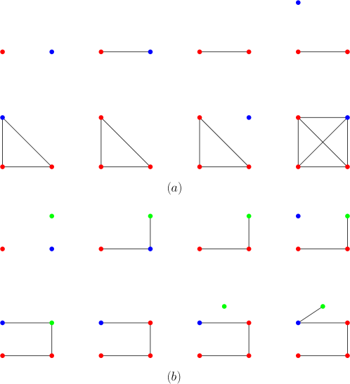
Figure 4: The operations for obtaining the clique-width of a graph, illustrated for (a) $K_{4}$, which has clique-width $2$, and (b) $P_{5}$, which has clique-width $3$.

3.4 Unbounded local clique-width

A $k$-labelled graph is a graph whose vertices are assigned integers (called labels) from $1$ to $k$ (each vertex has precisely one label). The clique-width of a graph $G$ equals the minimum $k$ such that $G$ can be obtained using the following four operations: creating a vertex labelled $1$, relabeling all vertices with label $i$ to label $j$, adding all edges between the vertices with label $i$ and the vertices with label $j$, and taking a disjoint union of graphs obtained using these operations (see Figure 4).

We say that a graph class ${\mathcal{C}}$ is of bounded local clique-width if there exists a function $g$ such that the following holds: for every graph $G\in{\mathcal{C}}$, integer $d$ and every vertex $x$ of $G$, the clique-width of the subgraph of $G$ induced on the vertices at distance $\leq d$ from $x$ in at most $g(d)$.

As noted above, the algorithm of [5] for MSO on graphs of bounded clique-width implies fixed-parameter tractability of FO model checking on graphs of bounded local clique-width via Gaifman’s locality. Though, the following opposite result was shown in [18] (note that the considered graph class has bounded diameter, and so claiming unbounded clique-width is enough):

Proposition 3.8 ([18, Proposition 5.2]).

For any irrational $q>0$ there is $\ell$ such that the subclass of interval graphs represented by intervals of lengths $1$ and $q$ on a line segment of length $\ell$ has unbounded clique-width.

This immediately implies unbounded local clique-width for classes of $2$-fold proper circular-arc graphs and also for similar subclasses of box and disk graphs, which justifies relevance of our new algorithms for FO model checking. Moreover, by an adaptation of the core idea of [18, Proposition 5.2] we can prove a much stronger negative result. We start with a claim capturing the essence of the construction in [18, Proposition 5.2].

Consider disjoint $m$-element vertex sets $X$ and $Y$ in a graph. We say that $X$ is gradually connected with $Y$ if there exist orderings $X=\{x_{1},x_{2},\dots,x_{m}\}$ and $Y=\{y_{1},y_{2},\dots,y_{m}\}$ such that, for any $i<j$, $x_{j}y_{i}$ is an edge while $x_{i}y_{j}$ is not an edge (we do not care about edges of the form $x_{i}y_{i}$). Recall that a transversal of a set system $\{X_{1},X_{2},\dots,X_{r}\}$ is a set $Z=\{z_{1},\dots,z_{r}\}$ of $r$ distinct elements such that $z_{i}\in X_{i}$ for $i=1,\dots,r$.

Lemma 3.9.

Let $k$ be an integer. Let $G$ be a graph and $V_{1},V_{2},\dots,V_{r}$ be a partition of the vertex set of $G$ such that $|V_{1}|=|V_{2}|=\dots=|V_{r}|=m$, and $m>6kr$. Assume that $V_{i}$ is gradually connected with $V_{i+1}$ for $i=1,2,\dots,r-1$. Furthermore, assume that there exists a set $I\subseteq\{1,\dots,r\}$, $|I|=2k$, such that the following holds: for any sets $X,Y$ such that $X$ is a transversal of the set system $\{V_{i}:i\in I\}$ and $Y$ is a transversal of $\{V_{i+1}:i\in I\}$, the set $X$ is gradually connected to $Y$. Then the clique-width of $G$ is at least $k$.

Proof.

Let $G$ be an assumed graph on $n=rm$ vertices, but the clique-width of $G$ is at most $k-1$. In the construction of $G$ using $k-1$ labels from the definition of clique-width, a $(k-1)$-labelled subgraph $G_{1}$ of $G$ with $\frac{1}{3}n\leq|V(G_{1})|\leq\frac{2}{3}n$ must have appeared. We will now get a contradiction by showing a set of $k$ vertices of $G_{1}$ which have pairwise different neighbourhoods in $G-V(G_{1})$.

Suppose that there exists $i$ such that $|V_{i+1}\cap V(G_{1})|-|V_{i}\cap V(G_{1})|\geq 2k$. Then there are sets $X\subseteq V_{i}\setminus V(G_{1})$ and $Y\subseteq V_{i+1}\cap V(G_{1})$, where $|X|=|Y|=2k$, such that $X$ is gradually connected to $Y$ with respect to orderings $X=\{x_{1},\dots,x_{2k}\}$ and $Y=\{y_{1},\dots,y_{2k}\}$. Then the vertices $y_{1},y_{3},\dots,y_{2k-1}$ of $G_{1}$ have pairwise different neighbourhoods in $G-V(G_{1})$, as witnessed by $x_{2},x_{4},\dots,x_{2k}$. The same applies if $|V_{i+1}\cap V(G_{1})|-|V_{i}\cap V(G_{1})|\leq-2k$.

The next step is to show that, for $i=1,\dots,r$, it holds $\emptyset\not=V_{i}\cap V(G_{1})\not=V(G_{1})$. Indeed, up to symmetry, let $V_{i}\cap V(G_{1})=\emptyset$ for some $i$, which implies $|V_{j}\cap V(G_{1})|<2kr<\frac{1}{3}m$ for all $j\in\{1,\dots,r\}$ by the previous paragraph, and the latter contradicts our assumption $|V(G_{1})|\geq\frac{1}{3}n$. For the assumed index set $I\subseteq\{1,\dots,r\}$, we can hence choose sets $X$ a transversal of $\{V_{i}:i\in I\}$ and $Y$ a transversal of $\{V_{i+1}:i\in I\}$, such that $X\cap V(G_{1})=\emptyset$ and $Y\subseteq V(G_{1})$. Moreover, $|X|=|Y|=2k$ and $X$ is gradually connected to $Y$ by the assumption of the lemma. We thus again get a contradiction as above. ∎

Proposition 3.10.

The following graph classes contain subclasses of bounded diameter and unbounded clique-width:

• unit circular-arc graphs of independence number $2$,

• circle graphs of independence number $2$,

• unit box and disk graphs with a representation contained within a square of bounded size.

                  

Figure 5: An illustration of the constructions used in the proof of Proposition 3.10. Left: unit circular-arc graphs for $m=3$ (this is not a valid value according to the proof, but proper $m=36k+1$ would not produce a comprehensible picture). Right: unit box graphs for $m=3$. The arcs/boxes in black colour represent the sets $V_{1},V_{4},V_{7},\dots$.

Proof.

Our overall aim is to construct special intersection representations of graphs within the claimed classes, which have bounded diameters and whose vertex sets can be partitioned into sets $V_{1},V_{2},\dots,V_{r}$ of properties assumed in Lemma 3.9. See also Figure 5.

First, consider the circle of radius $1$ and “unit” arcs of fixed length $a=(2\pi+\delta)/3$ on this circle, for a sufficiently small $\delta>0$. Since $3a$ is more than the circumference of the circle, there cannot be three disjoint arcs and the diameter of any such intersection graph is at most $3$. Choose $r=6k$ and $m=36k+1$, and let $\varepsilon$ be such that $0<\varepsilon<\delta/m$. Let $V_{1}$ consist of $m$ arcs of length $a$ starting at angles $0,\varepsilon,\dots,(m-1)\varepsilon$, and let $V_{i}$ for $i=2,\dots,r$ be a copy of $V_{1}$ shifted by the angle $(i-1)a$ counterclockwise. Clearly, $V_{i-1}$ is gradually connected with $V_{i}$. Moreover, $V_{4}$ is in fact a copy of $V_{1}$ shifted by the angle $\delta$ counterclockwise, and analogously with $V_{7},V_{10}$, etc. Assuming $(r+1)\delta<3$, this means that the whole set $V_{1}\cup\ V_{4}\cup\dots\cup V_{r-2}$ is gradually connected with $V_{2}\cup\ V_{5}\cup\dots\cup V_{r-1}$, and this implies the conditions of Lemma 3.9 with $I=\{1,4,\dots,r-2\}$. Since $k$ can be chosen arbitrary, our graphs have unbounded clique-width.

The same construction can be used in the second case as well; we simply replace each arc with a chord between the same ends, and this circle representation would represent an isomorphic graph to the previous case.

We have a similar construction also in the last two cases. We again choose $r=6k$, $m=36k+1$ and $0<\varepsilon<\delta/m$. Let the set $V_{1}$ consist of unit squares with the lower left corners at coordinates $(i\varepsilon,i\varepsilon)$ where $i=0,1,\dots,m-1$. Let $V_{2}$ be a copy of $V_{1}$ translated by the vector $(1,\delta)$ and $V_{3}$ be a copy of $V_{1}$ translated by $(\frac{1}{2},1+\delta)$. For $j=3,6,\dots,r-3$, let the triple $V_{j+1},V_{j+2},V_{j+3}$ be a copy of $V_{1},V_{2},V_{3}$ translated by $(\delta,\delta)$. Again, in the intersection graph, $V_{i-1}$ is gradually connected with $V_{i}$ for $i=1,2,\dots,r$. Assuming $(r+1)\delta<\frac{3}{2}$, we similarly fulfill the conditions of Lemma 3.9 with $I=\{1,4,\dots,r-2\}$, thus proving our claim of unbounded clique-width. One can also apply a similar construction in the case of unit disk graphs. ∎

4 Hardness for Intersection Classes

Our aim is to provide a generic reduction for proving hardness of FO model checking (even without labels on vertices) using only a simple property which is easy to establish for many geometric intersection graph classes. We will then use it to derive hardness of FO for quite restricted forms of intersection representations studied in our paper (Corollary 4.2).

We say that a graph $G$ represents consecutive neighbourhoods of order $\ell$, if there exists a sequence $S=(v_{1},v_{2},\dots,v_{\ell})\subseteq V(G)$ of distinct vertices of $G$ and a set $R\subseteq V(G)$, $R\cap S=\emptyset$, such that for each pair $i,j$, $1\leq i<j\leq\ell$, there is a vertex $w\in R$ whose neighbours in $S$ are precisely the vertices $v_{i},v_{i+1}\dots,v_{j}$. (Possible edges other than those between $R$ and $S$ do not matter.) A graph class ${\cal G}$ has the consecutive neighbourhood representation property if, for every integer $\ell>0$, there exists an efficiently computable graph $G\in{\cal G}$ such that $G$ or its complement $\overline{G}$ represents consecutive neighbourhoods of order $\ell$.

Note that our notion of ‘representing consecutive neighbourhoods’ is related to the concepts of “$n$-order property” and “stability” from model theory (mentioned in Section 1). This is not a random coincidence, as it is known [1] that on monotone graph classes stability coincides with nowhere dense (which is the most general characterization allowing for FPT FO model checking on monotone classes). In our approach, we stress easy applicability of this notion to a wide range of geometric intersection graphs and, to certain extent, to $\exists$FO model checking.

The main result is as follows. A duplication of a vertex $v$ in $G$ is the operation of adding a true twin $v^{\prime}$ to $v$, i.e., new $v^{\prime}$ adjacent to $v$ and precisely to the neighbours of $v$ in $G$.

Theorem 4.1.

Let ${\cal G}$ be a class of unlabelled graphs having the consecutive neighbourhood representation property, and ${\cal G}$ be closed on induced subgraphs and duplication of vertices. Then the FO model checking of ${\cal G}$ is $AW[*]$-complete with respect to the formula size.

Proof.

Our strategy is to prove that graphs in ${\cal G}$ can be used to represent any finite simple graph $H$ “via FO” – using an FO interpretation introduced in Section 2. To this end, we give a pair of FO formulas $I=(\nu,\psi)$ and for any graph $H$, we efficiently construct graphs $G_{H}\in{\cal G}$ and $H^{\prime}\simeq H$ such that $I(G_{H})=H^{\prime}$. Precisely, the last expression means $V(H^{\prime})=\{v:G_{H}\models\nu(v)\}$ and $E(H^{\prime})=\{uv:u,v\in V(H^{\prime}),\,G_{H}\models\psi(u,v)\vee\psi(v,u)\}$. Assuming this ($I(G_{H})=H^{\prime}\simeq H$) for a moment, we show how it implies the statement of the theorem.

Consider an FO model checking instance on ${\cal G}$, parameterized by an FO formula $\phi$. We assume input $H$, and $I$ and $G_{H}\in{\cal G}$ as above, and define an FO formula $\phi^{I}$ recursively (cf. Section 2): every occurrence of ${edge}(x,y)$ is replaced by $\psi(x,y)\vee\psi(y,x)$, every $\exists x\,\sigma$ is replaced by $\exists x\,(\nu(x)\wedge\sigma)$ and $\forall x\,\sigma$ by $\forall x\,(\nu(x)\to\sigma)$. Clearly, $G_{H}\models\phi^{I}\Longleftrightarrow H\models\phi$. The latter problem $H\models\phi$ is $AW[*]$-complete with respect to $|\phi|$ by Theorem 2.3. Since $|\phi^{I}|$ is bounded in $|\phi|$, we have got a parameterized reduction implying that the FO model checking problem of graphs from ${\cal G}$ is $AW[*]$-complete, too.

Now we return to the initial task of defining the FO interpretation $I=(\nu,\psi)$ and constructing $G_{H}\in{\cal G}$ for given $H$. Let $V(H)=\{1,2,\dots,n\}$. By the assumption, we can efficiently compute a graph $G_{n}\in{\cal G}$ that represents consecutive neighbourhoods of order $n+2$, as witnessed by a sequence $S=(v_{0},v_{1},\dots,v_{n},v_{n+1})\subseteq V(G_{n})$ and a set $R\subseteq V(G_{n})$. If it happened that, actually, the complement $\overline{G}_{n}$ represented consecutive neighbourhoods, then we would simply switch to $\neg edge(x,y)$ in the formulas below.

For $0\leq i<j\leq n$, let $r_{i,j}\in R$ denote a vertex whose neighbours in $S$ are precisely $v_{i},v_{i+1}\dots,v_{j}$. Let $P:=\{r_{0,1},r_{1,2},\dots,r_{n,n+1}\}$ and $Q:=\{r_{i,j}:ij\in E(H)\}$ (it may happen that $P\cap Q\not=\emptyset$, but $S\cap(P\cup Q)=\emptyset$). We construct $G_{H}$ as the subgraph of $G_{n}$ induced on the vertex set $S\cup P\cup Q$. By the assumption that ${\cal G}$ is closed on induced subgraphs, we have got $G_{H}\in{\cal G}$. Furthermore, we give labels ‘$blue$’ to every vertex of $S$, ‘$green$’ to every vertex of $P$ and ‘$red$’ to every vertex of $Q$ (those in $P\cap Q$ get both ‘$green$’ and ‘$red$’).

Using the labels, construction of the desired FO interpretation is now easy;

$$\nu(x) \equiv\>blue(x)\wedge\exists s,s^{\prime}\big{(}s\not=s^{\prime}\wedge green(s)\wedge green(s^{\prime})\wedge edge(x,s)\wedge edge(x,s^{\prime})\big{)},$$ (4)

$$\psi(x,y) \equiv\>blue(x)\wedge blue(y)\wedge x\not=y\wedge\exists z\big{[}red(z)\wedge extreme(x,z)\wedge extreme(y,z)\big{]},$$

where $\nu(x)$ is true precisely for $v_{1},\dots,v_{n}$ of $S$, and $extreme(x,z)$ in $\psi$ means that $x$ is one of the “extreme” neighbours of $z$ within the sequence $S$. The point is that we can express the latter in FO with help of the ‘$green$’ vertices which define the (symmetric) successor relation of $S$ within the graph $G_{H}$. It is

$$extreme(x,z)\equiv~{} edge(x,z)$$

$$\wedge\exists s,x^{\prime}\big{[}green(s)\wedge blue(x^{\prime})\wedge edge(x,s)\wedge edge(s,x^{\prime})\wedge\neg edge(x^{\prime},z)\big{]},$$

where the second line states that $x$ is connected to blue $x^{\prime}$ via a green vertex, such that $x^{\prime}$ is not a neighbour of $z$. Altogether, for $I=(\nu,\psi)$ we easily verify $I(G_{H})\simeq H$ (where the isomorphism maps each blue vertex $v_{i}$ to $i\in V(H)$).

The last step shows how we can get rid of the labels. For that we use duplication of vertices (which preserves membership in ${\cal G}$ by the assumption). For start, notice that no two vertices of $G_{H}$ can be twins by our construction. Then every vertex in $P\setminus Q$ is duplicated once, every vertex in $P\cap Q$ is duplicated twice and every in $Q\setminus P$ is duplicated three times, forming the new graph $G_{H}^{\prime}\in{\cal G}$.

Regarding the formulas of $I$, we apply a corresponding transformation. Start with a formula $twin(x,y)\equiv edge(x,y)\wedge\forall z[(z\neq x\wedge z\neq y)\rightarrow(edge(x,z)\leftrightarrow edge(y,z))]$ asserting that $x,y$ are true twins. We can routinely write down formulas $dupl_{d}(x)$ asserting that the vertex $x$ is a part of a class of $\geq d$ true twins, e.g., $dupl_{2}(x)\equiv\exists z(z\not=x\wedge twin(x,z))$ and $dupl_{3}(x)\equiv\exists z,z^{\prime}(x\not=z\not=z^{\prime}\not=x\wedge twin(x,z)\wedge twin(x,z^{\prime}))$. Then we transform $I=(\nu,\psi)$ into $I^{\prime}=(\nu^{\prime},\psi^{\prime})$ as follows

• $blue(x)$ is replaced with $\neg dupl_{2}(x)$,

• $green(x)$ is replaced with $dupl_{2}(x)\wedge\neg dupl_{4}(x)$,

• $red(x)$ is replaced with $dupl_{3}(x)$, and

• $x=y$ is replaced with $twin(x,y)$.

One can routinely verify that again $I^{\prime}(G_{H}^{\prime})\simeq H$. Moreover, $G_{H}^{\prime}\in{\cal G}$ has been constructed in polynomial time from $H$, and $G_{H}^{\prime}$ carries no labels. ∎

                  

Figure 6: Constructing witnesses of the consecutive neighbourhood representation property – as permutation graphs (left) and as unit-box graphs (right); cf. Corollary 4.2.

Graphs witnessing the consecutive neighbourhood representation property can be easily constructed within our intersection classes, even with strong further restrictions. See some illustrating examples in Figure 6. So, we obtain the following hardness results:

Corollary 4.2.

The FO model checking problem is $AW[*]$-complete with respect to the formula size, for each of the following geometric graph classes (all unlabelled):
a) circular-arc graphs with a representation consisting or arcs of lengths from $[\pi-\varepsilon,\pi+\varepsilon]$ on the circle of diameter $1$, for any fixed $\varepsilon>0$,
b) connected permutation graphs,
c) unit-box graphs with a representation contained within a square of side length $2+\varepsilon$, for any fixed $\varepsilon>0$,
d) unit-disk graphs (that is of diameter $1$) with a representation contained within a rectangle of sides $1+\varepsilon$ and $2$, for any fixed $\varepsilon>0$.

Proof.

Each of the considered graph classes is routinely closed under induced subgraphs and duplication. Hence it is enough to construct, in each of the classes, appropriate witnesses of the consecutive neighbourhood representation property.

a) For an integer $n$ and $\delta:=\varepsilon/2n$, we consider the sets of arcs ${\cal S}=\{[i\delta,\pi+i\delta]:i=1,2,\dots,n\}$ and ${\cal N}=\{[\pi+j\delta+\frac{\delta}{2},\,i\delta-\frac{\delta}{2}]:1\leq i<j\leq n\}$. The complement of the circular-arc intersection graph of ${\cal S}\cup{\cal N}$ represents consecutive neighbourhoods of order $n$.

b) Let $x,y$ be two parallel lines. We represent the line segments of a permutation representation on $x,y$ by pairs $\langle x_{i},y_{i}\rangle$ where $x_{i},y_{i}$ are the coordinates of the two ends on the lines $x,y$ respectively. Our witness of order $n$ simply consists of the sets ${\cal S}=\{\langle i,i\rangle:i=1,2,\dots,n\}$ and ${\cal N}=\{\langle i-\frac{1}{2},j+\frac{1}{2}\rangle:1\leq i<j\leq n\}$, as roughly depicted in Figure 6.

c) As illustrated in Figure 6, we specify ${\cal S}$ as the set of unit boxes $B_{i}$ with their lower corners at coordinates $(i\delta,(n-i)\delta)$ where $i=1,2,\dots,n$ and $\delta:=\varepsilon/n$. For any $1\leq i<j\leq n$, we introduce a unit box with the lower left corner at $(1+i\delta-\frac{\delta}{2},1+(n-j)\delta-\frac{\delta}{2})$, which intersects exactly $B_{i},B_{i+1},\dots,B_{j}$. Let ${\cal N}$ denote the set of the latter boxes; then the intersection graph of ${\cal S}\cup{\cal N}$ represents consecutive neighbourhoods of order $n$.

d) We take the set ${\cal S}$ of unit disks $D_{i}$ (of diameter $1$) with their centers at coordinates $(i\delta,0)$ where $i=1,2,\dots,n$ and $\delta:=\varepsilon/n$. Then, let ${\cal N}$ consists of the unit disks $D^{\prime}_{i,j}$, for all $1\leq i<j\leq n$, with centers at the coordinates $(\frac{1}{2}(i+j)\delta,h_{j-i})$ where $h_{d}<1$ is a suitable rational (of small size) such that $h_{d}^{2}+\frac{1}{4}(d\delta)^{2}<1$ and $h_{d}^{2}+\frac{1}{4}(d\delta+\delta)^{2}>1$. Note that $D^{\prime}_{i,j}$ intersects exactly $D_{i},D_{i+1},\dots,D_{j}$, and so the intersection graph of ${\cal S}\cup{\cal N}$ represents consecutive neighbourhoods of order $n$. ∎

It is worthwhile to notice that for each of the classes listed in Corollary 4.2, the $k$-clique and $k$-independent set problems are all easily FPT, and yet FO model checking is not.

Finally, we return to the weaker $\exists$FO model checking problem. In fact, this problem can be treated “the same” as the aforementioned parameterized induced subgraph isomorphism problem, which is a folklore result whose short proof we include for the sake of completeness:

Proposition 4.3.

On any class ${\cal G}$ of simple unlabelled graphs, the parameterized problems of induced subgraph isomorphism and of $\exists$FO model checking are equivalent regarding FPT. Precisely, one of them admits an FPT algorithm on ${\cal G}$ if and only if the other does so.

Proof.

In one direction, given a graph $H$, $|V(H)|=k$, we straightforwardly construct a quantifier-free FO formula $\phi_{H}(x_{1},\dots,x_{k})$ such that $G\models\phi_{H}(x_{1},\dots,x_{k})$ iff $G[x_{1},\dots,x_{k}]$ is isomorphic to $H$, and $|\phi_{H}|$ is bounded in $k$. Then $\exists x_{1},\dots,x_{k}\>\phi_{H}(x_{1},\dots,x_{k})$ is an $\exists$FO sentence solving the $H$-induced subgraph isomorphism problem on ${\cal G}$.

In the other direction, assume an $\exists$FO formula $\psi\equiv\exists x_{1},\dots,x_{k}\>\psi_{1}(x_{1},\dots,x_{k})$ where $\psi_{1}$ is quantifier-free. For a fixed vertex set $V=\{v_{1},\dots,v_{k}\}$ (note; some vertices in this list might be identical), let ${\cal H}_{\psi}$ denote the finite set of all simple graphs on $V$ such that $\psi_{1}(v_{1},\dots,v_{k})$ holds true for them. Then the $\psi$-model checking problem on a graph $G$ reduces to checking whether, for some $H\in{\cal H}_{\psi}$, the pair $\langle G,H\rangle$ is a Yes instance of induced subgraph isomorphism. Since $|{\cal H}_{\psi}|$ is bounded in $k\leq|\psi|$, the result follows. ∎

The hardness construction in the proof of Theorem 4.1 can be turned into $\exists$FO, but only if vertex labels are allowed (notice that in the proof, we introduced the universal quantifier only when we had to remove the labels). Though, we can modify some of the constructions from Corollary 4.2 to capture also $\exists$FO without labels.

Proposition 4.4.

The $\exists$FO model checking problem is $W[1]$-hard with respect to the formula size, for both the following unlabelled geometric graph classes:
a) circle graphs,
b) unit-box graphs with a representation contained within a square of side length $3$.

Proof.

In the proof we carefully combine the respective constructions from Corollary 4.2 with the first part of the proof of Theorem 4.1, so that universal quantifiers are avoided – this way we get the interpretation (4) $I=(\nu,\psi)$ (labelled) which is actually $\exists$FO. Recall that $I$ is capable of interpreting any simple graph $H$ in a suitable graph $G_{H}$ constructed in the considered class in polynomial time, that is, $H\simeq I(G_{H})$.

Then, in each of the considered cases, we will show an ad hoc modification of the construction (see below) with the benefit of removing the colour labelling. Before giving details of the modifications, we show how the proof of $W[1]$-hardness is to be finished.

Consider the $\exists$FO formula

$$\gamma_{k}\>\equiv\>\exists x_{1},\dots,x_{k}\left[\bigwedge_{1\leq i\leq k}\nu(x_{i})\wedge\!\!\bigwedge_{1\leq i<j\leq k}\!\!x_{i}\not=x_{j}\wedge\!\!\bigwedge_{1\leq i<j\leq k}\!\!\big{(}\psi(x_{i},x_{j})\vee\psi(x_{j},x_{i})\big{)}\right];$$

by the assumed interpretation, $G_{H}\models\gamma_{k}$ if and only if $H$ contains $k$ vertices forming a clique, where the latter is a $W[1]$-hard problem with respect to $k$. Since $|\gamma_{k}|$ is bounded in $k$, this implies that the $\exists$FO model checking instance $G_{H}\models\gamma_{k}$ is also $W[1]$-hard with respect to $|\gamma_{k}|$, where $G_{H}$ is restricted to the considered graph class.

It remains to provide the ad hoc modified constructions and the corresponding modifications of the formulas $\nu,\psi$ in $\gamma_{k}$.

a) We turn the permutation witness (of consecutive neighbourhoods) from Corollary 4.2b) into a circle representation by joining the two parallel lines into one circle. We then observe that no odd cycle $C_{2a+1}$ for $a\geq 2$ is a permutation graph since it does not have a transitive orientation, but every odd cycle has a straightforward overlap representation. Hence, if one wants to label a chord of a circle representation, it is possible to do so by adding an adjacent small subrepresentation of an odd cycle.

Namely, let ${\cal D}$ be the labelled circle representation of $G_{H}$ constructed for given $H$ in the proof of Theorem 4.1. For each chord $a$ of ${\cal D}$ which has received label ‘$blue$’, we add a fresh copy of (the representation of) $C_{5}$ with one vertex adjacent to $a$. We analogously add an adjacent copy of $C_{7}$ for every ‘$red$’ chord and of $C_{9}$ for every ‘$green$’ chord. Let ${\cal D}^{\prime}$ denote the new (unlabelled) circle representation and $G_{H}^{\prime}$ its intersection graph. Since $G_{H}$ is actually a permutation graph by Corollary 4.2b), the only induced $C_{5},C_{7},C_{9}$ in $G_{H}^{\prime}$ are those later added ones. Consequently, it is a routine task to express the predicate $blue(x)$ in $\exists$FO as ‘there exist vertices inducing $C_{5}$, and one is adjacent to $x$’, and likewise for $red(x)$ and $green(x)$. In this way, we get from $\gamma_{k}$ an $\exists$FO formula $\gamma_{k}^{\prime}$ such that $G_{H}\models\gamma_{k}$ if and only if $G_{H}^{\prime}\models\gamma_{k}^{\prime}$.

Figure 7: Replacing explicit labels in the hardness construction of Proposition 4.4b) – adding the three black and several green boxes to the illustration in Figure 6 right.

b) This time we are not able to add “local markers” as in a), since all boxes need to be of the same size. Instead, we add just several new boxes to the whole unit-box representation ${\cal B}$ from Corollary 4.2c). See Figure 7; the three black boxes are added to intersect precisely all the original blue boxes, and one intersecting green box is added to every red box which, in the proof of Theorem 4.1, represents the successor relation on blue boxes (that is, which has received also label ‘$green$’).

As one can easily check from the picture, we can now express the predicate $blue(x)$ using $\exists$FO as ‘there exist four independent neighbours of $x$’ (this property is false for every other box type here). Similarly, $red(x)$ can be expressed as ‘there exists a blue box adjacent to $x$ and a blue box not adjacent to $x$’. Finally, $green(x)$ should be true for those red boxes which have a green neighbour box, where a green box is characterised as having a blue and a red non-neighbour.

The proof is then finished in the same way as in case a). ∎

One complexity question that remains open after Proposition 4.4 is about $\exists$FO on unlabelled permutation graphs (for labelled ones, this is $W[1]$-hard by the remark after Corollary 4.2). While induced subgraph isomorphism is generally NP-hard on permutation graphs by [24], we are not aware of results on the parameterized version, and we currently have no plausible conjecture about its parameterized complexity.

5 Polygonal Visibility Graphs

5.1 Definitions

Given a polygon $W$ in the plane, two vertices $p_{i}$ and $p_{j}$ of $W$ are said to be mutually visible if the line segment $p_{i}p_{j}$ does not intersect the exterior of $W$. The visibility graph $G$ of $W$ is defined to have vertices $v_{i}$ corresponding to each vertex $p_{i}$ of $W$, and edge $(v_{i},v_{j})$ if and only if $p_{i}$ and $p_{j}$ are mutually visible.

Visibility graphs have been studied for several subclasses of polygons, such as orthogonal polygons, spiral polygons etc [13, 23, 11]. Our aim is to study the visibility graphs of some special established classes of polygons with respect to FO model checking.

If there is an edge $e$ of the polygon $W$, such that for any point $p$ of $W$, there is a point on $e$ that sees $p$, then $W$ is called a weak visibility polygon, and $e$ is called a weak visibility edge of $W$ (Figure 8a) [19, 20]. A vertex $v_{i}$ of $W$ is called a reflex vertex if the interior angle of $W$ formed at $v_{i}$ by the two edges of $W$ incident to $v_{i}$ is more than $\pi$. Otherwise, $v_{i}$ is called a convex vertex. If both of the end vertices of an edge of $W$ are convex vertices, then the edge is called a convex edge.

If the boundary of $W$ consists only of an x-monotone polygonal arc touching the x-axis at its two extreme points, and an edge contained in the x-axis joining the two points, then it is called a terrain (Figure 8b) [19, 12]. All terrains are weak visibility polygons with respect to their edge that lies on the x-axis. If all points of a $W$ are visible from a single vertex $v$ of the polygon, then $W$ is called a fan (Figure 8c) [19, 21]. If $W$ is a fan with respect to a convex vertex $v$, then $W$ is called a convex fan [28]. If $W$ is a convex fan with respect to a vertex $v$, then both of the edges of $W$ incident to $v$ are convex edges, and $W$ is also a weak visibility polygon with respect to any of them.

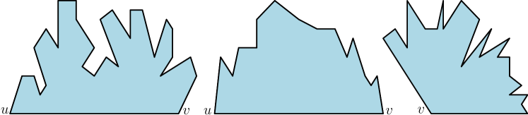
Figure 8: From left to right: (a) a weak visibility polygon with respect to edge $uv$; (b) a terrain; (c) a convex fan visible from the vertex $v$.

In this section we identify some interesting tractable and hard cases of the FO model checking problem on these visibility classes.

5.2 Hardness for terrain and convex fan visibility graphs

We first argue that the FO model checking problem of polygon visibility graphs stays hard even when the polygon is a terrain and a convex fan. Our approach is very similar to that in Theorem 4.1 above, that is, we show that a given FO model checking instance of general graphs can be interpreted in another instance of the visibility graph of a specially constructed polygon which is a terrain and a convex fan at the same time. However, since polygon visibility graphs are in general not closed on induced subgraphs and duplication of vertices, we have to reformulate all the arguments from scratch.

Theorem 5.1.

The FO model checking problem of unlabelled polygon visibility graphs (given alongside with the representing polygon) is $AW[*]$-complete with respect to the formula size, even when the polygon is a terrain and a convex fan at the same time.

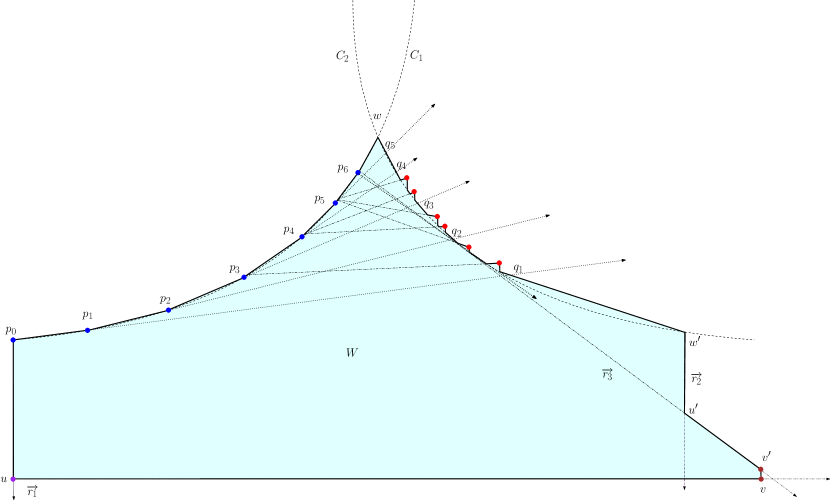
Figure 9: The constructed polygon for a graph with $n=5$ vertices and edges $(v_{1},v_{3})$, $(v_{1},v_{5})$, $(v_{2},v_{4})$, $(v_{2},v_{5})$, $(v_{3},v_{4})$ and $(v_{3},v_{5})$. The purple vertex $u$ sees all vertices of $W$, while the brown vertices $v$ and $v^{\prime}$ see only $u$, $u^{\prime}$, all the blue vertices and each other. Each blue vertex $p_{i}$, $1\leq i\leq 5$ represents the vertex $v_{i}$ of the graph.

Proof.

Consider a given graph $H$ with $n$ vertices and $m$ edges. We construct our polygon $W$ as follows (see Figure 9): Consider an increasing, convex curve $C_{1}$ with respect to the x-axis. We mark $n+3$ points $p_{0},p_{1},p_{2},\ldots,p_{n},p_{n+1}$ and $w$ on $C_{1}$ from left to right. Each of the points will later be a vertex of the polygon, and $p_{i}$, $1\leq i\leq n$ will represent the vertices $v_{i}$ of the given graph $H$.

From $w$ onwards, we consider a decreasing convex curve $C_{2}\ni w$. For each ray $\overrightarrow{p_{i-1}p_{i}}$, $1\leq i\leq n+1$, denote the point of intersection of $C_{2}$ and $\overrightarrow{p_{i-1}p_{i}}$ by $q_{i}$. In the arc of $C_{2}$ between $q_{i}$ and $q_{i+1}$, we arbitrarily choose $n$ pairwise disjoint subarcs $D_{i,j}$, $1\leq j\leq n$, of positive length. Now, for each edge $e_{k}=(v_{i},v_{j})\in E(H)$, $i<j$, we choose a point $s^{1}_{k}\in C_{2}$ arbitrarily in the interior of $D_{i,j}$. From a point slightly above $p_{j}$ on $C_{1}$, we start a ray that intersects $C_{2}$ at $s^{1}_{k}$. Now we mark a second point $s^{2}_{k}$ on this ray a tiny distance to the right of $s^{1}_{k}$ (notice that $s^{2}_{k}$ is slightly above $C_{2}$). Finally, we drop a vertical ray downward from $s^{2}_{k}$ to intersect $C_{2}$ at a third point $s^{3}_{k}$. Note that these distances should be so small that also $s^{3}_{k}$ belongs to $D_{i,j}$. This ensures that among the $p_{i}$’s, $s^{2}_{k}$ sees exactly all points $p_{i},p_{i+1},\ldots,p_{j}$, and $s^{2}_{k}$ is visible from any point below itself to the left.

To finish the construction of $W$, we mark a point $w^{\prime}$ on $C_{2}$ to the right of all the points marked so far. We drop two vertical rays $\overrightarrow{r_{1}}$ and $\overrightarrow{r_{2}}$ downward from $p_{0}$ and $w^{\prime}$ respectively. We consider a point slightly above $p_{n+1}$ on $C_{1}$ and draw the lower tangent $\overrightarrow{r_{3}}$ from it to $C_{2}$. Denote the point of intersection of $\overrightarrow{r_{2}}$ and $\overrightarrow{r_{3}}$ as $u^{\prime}$. Intersect $\overrightarrow{wp_{n+1}}$ with $\overrightarrow{r_{1}}$, say, at point $x$. Intersect $\overrightarrow{r_{1}}$ and $\overrightarrow{r_{3}}$ with a horizontal line below both $x$ and $u^{\prime}$. Denote the point of intersection of $\overrightarrow{r_{1}}$ and the horizontal line as $u$. Mark a point $v$ slightly to the left of the intersection of the horizontal line and $\overrightarrow{r_{3}}$, so that $v$ cannot see any point on $C_{2}$. Mark another point $v^{\prime}$ vertically slightly above $v$ on $\overrightarrow{r_{3}}$.

Now we draw the polygon by starting from $p_{0}$ and drawing the polygonal boundary by connecting successive points embedded on $C_{1}$ and then $C_{2}$ (including points $s^{2}_{k}$) from left to right. We complete $W$ by connecting with edges the remaining points in the sequence $(w^{\prime},u^{\prime},v^{\prime},v,u,p_{0})$. We summarise the properties of the resultant polygon $W$ and its visibility graph $G$:

• $W$ is a terrain with respect to $uv$ and a convex fan with respect to $v$,

• no two points among $\{p_{0},p_{1},\ldots,p_{n+1}\}$ see each other except the consecutive pairs,

• for every $1\leq k\leq m$, the points $s^{1}_{k},s^{3}_{k}$ see a consecutive strip of $\{p_{0},p_{1},\ldots,p_{n+1}\}$ including $p_{n+1}$, while $s^{2}_{k}$ can see $p_{i},p_{i+1},\ldots,p_{j}$ but neither $p_{i-1},p_{j+1}$ nor $p_{n+1}$, and

• the vertices $v$ and $v^{\prime}$ are true twins in $G$ – they see the same neighbourhood which (except $v,v^{\prime}$) is $\{p_{0},p_{1},\ldots,p_{n+1},u,u^{\prime}\}$, and there is no other twin pair in $G$.

Claim 5.2.

Construction of the polygon $W$ can be finished in polynomial time.

Since the constructed visibility graph $G$ is clearly of polynomial size with respect to given $H$, we only need to show that we can finish our construction of $W$ with rational coordinates of sufficiently small size. To argue this, we choose suitable curves $C_{1},C_{2}$ such as quadratic functions $y=(x+c)^{2}$ for appropriate values of $c$. We pick $p_{0},p_{1},\ldots,p_{n},p_{n+1}$ and $w$ as grid points on $C_{1}$. The positions of $q_{1},\dots,q_{n+1}$ are computed only approximately (they are not vertices of $W$ anyway), and then we choose the subarcs $D_{i,j}$ with suitable (small) rational coordinates. Subsequent choices of $s^{1}_{k},s^{2}_{k},s^{3}_{k}$ can also be done with rational coordinates of small size, for $1\leq k\leq m$. The remaining vertices of $W$ follow easily.

Claim 5.3.

There exists a pair of FO formulas $I=(\nu,\psi)$ (an FO interpretation) such that, for any given graph $H$, the resultant visibility graph $G$ (as above) satisfies $H\simeq I(G)$.

We stress that the graph $G$ we have constructed is unlabelled, but for clarity we will refer to the vertex colours introduced in Figure 9. Recall, from the proof of Theorem 4.1, the formula $twin(x,y)\equiv edge(x,y)\wedge\forall z[(z\neq x\wedge z\neq y)\rightarrow(edge(x,z)\leftrightarrow edge(y,z))]$ asserting that $x,y$ are true twins. Since $v,v^{\prime}$ are the only twins in $G$, we may match either of them with the formula

$$brown(x)\>\equiv\>\exists t\,x\not=t\wedge twin(x,t).$$

Subsequently, the vertices $p_{0},p_{1},\ldots,p_{n+1}$ are precisely those matched by the formula

$$blue(x)\>\equiv\>\exists z\big{[}brown(z)\wedge edge(x,z)\wedge\exists t(edge(t,z)\wedge\neg edge(t,x))\big{]}$$

since, among all the neighbours of $v$, the vertices $u,u^{\prime}$ see all the other neighbours of $v$.

The vertex set of $H$ (in the interpretation $I$) can hence be defined using

$$\nu(x)\>\equiv\>blue(x)\wedge\exists z,z^{\prime}\big{(}z\not=z^{\prime}\wedge blue(z)\wedge blue(z^{\prime})\wedge edge(x,z)\wedge edge(x,z^{\prime})\big{)},$$

which excludes $p_{0}$ and $p_{n+1}$ from the list of blue points. Recall that every edge $e_{k}=(v_{i},v_{j})\in E(H)$, $i<j$, is represented by the red vertex $s^{2}_{k}$ which sees precisely $p_{i},p_{i+1},\dots,p_{j}$ among the blue points. Our aim, in the formula $\psi(x,y)$ of $I$, is to specify that $x=p_{i}$ and $y=p_{j}$ (or vice versa), and this can be done by referring to the unique blue neighbours $p_{i-1}$ and $p_{j+1}$ of $x$ and $y$, respectively, which do not see $s^{2}_{k}$. (This part is the reason why we use blue $p_{0},p_{n+1}$ in our construction.) We write down this as follows

$$\psi(x,y)\>\equiv\> blue(x)\wedge blue(y)\wedge\>\exists z,t,t^{\prime}\big{[}\,blue(t)\wedge blue(t^{\prime})\wedge edge(x,t)\wedge edge(y,t^{\prime})$$

$$\wedge\neg blue(z)\wedge edge(x,z)\wedge edge(y,z)\wedge\neg edge(t,z)\wedge\neg edge(t^{\prime},z)\big{]}.$$

Then $G\models\psi(v_{i},v_{j})$ if, and only if, $(v_{i},v_{j})\in E(H)$.

The rest of the proof is as in Theorem 4.1. ∎

5.3 Visibility graphs of weak visibility polygons of convex edges

In this section we prove that FO model checking of the visibility graph of a given weak visibility polygon of a convex edge is FPT when additionally parameterized by the number of reflex vertices. We remark that, for example, the independent set problem is NP-hard on polygonal visibility graphs [30], but Ghosh et al. [20] showed that the maximum independent set of the visibility graph of a given weak visibility polygon of a convex edge, is computable in quadratic time. In Theorem 5.1, we have seen that the latter result does not generalise to arbitrary FO properties, since FO model checking remains hard even for a very special subcase of weak visibility polygons. So, an additional parameterization in the next theorem is necessary.

Theorem 5.4.

Let $W$ be a given polygon weakly visible from one of its convex edges, with $k$ reflex vertices, and let $G$ be the visibility graph of $W$. Then FO model checking of $G$ is FPT with respect to the parameters $k$ and the formula size.

Before diving into the technical details of the rather long proof, we first provide a brief informal summary of the coming steps. As in the previous intersection graph cases, our aim is to construct, from given $W$, a poset ${\cal P}$ such that the width of ${\cal P}$ is bounded by a function of $k$ and that we have an FO interpretation of the visibility graph of $W$ in this ${\cal P}$.

Let $W$ be weakly visible from its convex edge $uv$, and denote by $C_{uv}$ the clockwise sequence of the vertices of $W$ from $u$ to $v$. The subsequence of $C_{uv}$ between two reflex vertices $v_{a}$ and $v_{b}$, such that all vertices in it are convex, is called an ear of $W$. The length of this sequence can be $0$ as well. Additionally, the first (last) ear of $W$ is defined as the subsequence between $u$ and the first reflex vertex of $C_{uv}$ (between the last reflex vertex and $v$, respectively). We have got $k+1$ ears in $W$. With a slight abuse of terminology at $u,v$, we may simply say that an ear is a sequence of convex vertices between two reflex vertices.

The crucial idea of our construction of the poset ${\cal P}$ (which contains all vertices of $W$, in particular) is that the visibility edges between the internal (convex) vertices of the ears are nicely structured: withing one ear $E_{a}$, they form a clique, and between two ears $E_{a},E_{b}$, the visibility edges exhibit a “shifting pattern” not much different from the left and right ends of intervals in a proper interval representation (cf. Lemma 3.2). Consequently, we may “encode” all the edges between $E_{a}$ and $E_{b}$ with help of an extra subposet of ${\cal P}$ of fixed width, and since we have got only $k+1$ ears, this together gives a poset of width bounded in $k$.

The last step concerns visibility edges incident with one of the $k$ reflex vertices or $u,v$. These can be easily encoded in ${\cal P}$ with only $2(k+2)$ additional labels, without any assumption on the structure of ${\cal P}$: for each reflex vertex $x$ of $C_{uv}$, or $x\in\{u,v\}$, we assign one new label $L^{0}_{x}$ to $x$ itself and another new label $L^{1}_{x}$ to all the neighbours of $x$. Altogether, we can efficiently construct an FO interpretation of $G$ in ${\cal P}$ such that the formulas depend only on $k$. Then we may finish by Theorem 2.1.

Proof of Theorem 5.4.

Throughout the proof (rest of the section) we will implicitly assume a polygon $W$ which is weakly visible from its edge $uv$, where $uv$ is a convex edge of $W$, and the clockwise boundary from $u$ to $v$, denoted as $C_{uv}$, contains all the other edges of $W$. We also recall that $C_{uv}$ consists of $k+1$ ears. Let $G=(V,E)$ be the visibility graph of $W$.

We need more terminology and some specialised claims.

For two elements $p,q$ of a poset, we say that $q$ covers $p$ if $p\sqsubseteq q$ and there is no poset element $r$ such that $p\sqsubseteq r\sqsubseteq q$ and $p\not=r\not=q$.

A vertex $z$ of $w$ is said to block two vertices $v_{i}$ and $v_{j}$ of $W$ if the shortest path between $v_{i}$ and $v_{j}$ that does not intersect the exterior of $W$, takes a turn at $z$. For two vertices $a$ and $b$ of $W$, when we say $a$ precedes $b$ or $b$ succeeds $a$ on $C_{uv}$, we mean that we encounter $a$ earlier than $b$ when we traverse $C_{uv}$ in the clockwise order, starting from $u$.

Claim 5.5.

Let $E_{a}$ and $E_{b}$ be two ears of $W$ such that $E_{a}$ precedes $E_{b}$ on $C_{uv}$. Let $v_{a}$ and $v_{b}$ be any convex vertices of $E_{a}$ and $v_{i}$ and $v_{j}$ be any convex vertices of $E_{b}$, where $v_{a}$ precedes $v_{b}$ and $v_{i}$ precedes $v_{j}$ on $C_{uv}$. Then the following hold. If $v_{a}$ sees $v_{i}$, then $v_{a}$ also sees $v_{j}$. Symmetrically, if $v_{j}$ sees $v_{b}$, then $v_{j}$ also sees $v_{a}$.

Proof.

Suppose that $v_{a}$ does not see $v_{j}$. Then there must be a blocker of $v_{a}$ and $v_{j}$. Since $v_{i}$ and $v_{j}$ are convex vertices of the same ear, the blocker cannot come from the polygonal boundary in between them. Since the $v_{a}v_{i}$ lies inside $W$, the blocker also cannot come from the clockwise polygonal boundary between $v_{a}$ and $v_{i}$. If the blocker comes from the clockwise polygonal boundary between $u$ and $v_{a}$ then $v_{a}$ cannot see any part $uv$, a contradiction. Similarly, the blocker cannot come from the clockwise polygonal boundary between $v_{j}$ and $v$ as well. So, $v_{a}$ must see $v_{j}$. The second claim follows from symmetrical arguments. ∎

Now we describe our construction of the poset ${\cal P}=(P,\leq^{\cal P})$ where $P$ includes the vertices $V$ of $W$. We start with a linear order $\leq^{C}$ on the vertex set $V$ defined as follows. For two vertices $a$ and $b$ of $V$, we let $a\leq^{C}b$ iff $a$ precedes $b$ in the clockwise order on $C_{uv}$ or $a=b$. We give all elements of $V$ label ‘$green$’ and, additionally, give label ‘$black$’ to those which are reflex vertices of $W$ and to $u,v$. Let $\leq^{C}$ be a subrelation of $\leq^{\cal P}$. We have:

Claim 5.6.

It can be expressed in FO that two vertices of $C_{uv}$ belong to the same ear.

Proof.

We give the formula

$$\beta_{0}(x,y)\equiv green(x)\wedge green(y)\wedge x\leq^{\cal P}\!y\wedge\,\forall z\left[(x\leq^{\cal P}\!z\wedge z\leq^{\cal P}\!y\wedge black(z))\rightarrow(z=x\vee z=y)\right]$$

and use its symmetric closure $\beta_{0}(x,y)\vee\beta_{0}(y,x)$. ∎

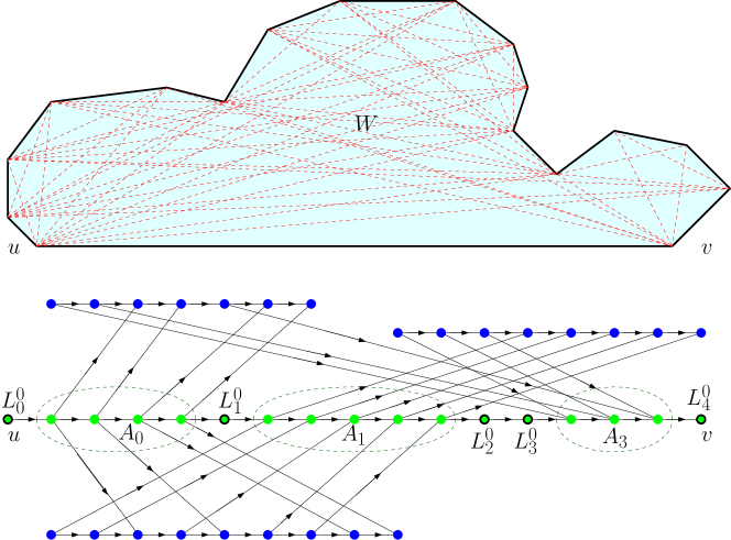
Figure 10: An illustration of a weak visibility polygon $W$ and its constructed poset, as in the proof of Theorem 5.4. Here, the sequence $C_{uv}$ (the green chain of the poset) consists of four ears $E_{0},E_{1},E_{2},E_{3}$ with interiors $A_{0},A_{1},A_{2},A_{3}$, where $A_{2}$ is empty (has no convex vertices). So, there are three blue chains (top to bottom) $B_{0,3},B_{1,3},B_{0,1}$ in the picture. The dashed lines in $W$ are the visibility edges of $G$.

Next, we number the ears of $C_{uv}$ as $E_{0},E_{1},\dots,E_{k}$ in the clockwise order. For every pair $0\leq a<b\leq k$, we now describe a subposet of ${\cal P}$ which we will use to encode the edges between the convex vertices of $E_{a}$ and $E_{b}$. Let $A_{a}$ and $A_{b}$ be the sets of convex vertices of $E_{a}$ and $E_{b}$, respectively, and let $B_{a,b}$ denote a fresh disjoint copy of $(A_{a}\cup A_{b})$. For each $v_{i}\in A_{a}$ and its corresponding copy $v_{i}^{\prime}\in B_{a,b}$, we have $v_{i}\leq^{\cal P}v_{i}^{\prime}$. Analogously, for each $v_{j}\in A_{b}$ and its corresponding copy $v_{j}^{\prime}\in B_{a,b}$, we have $v_{j}^{\prime}\leq^{\cal P}v_{j}$ and, in fact, it holds that $v_{i}^{\prime}$ covers $v_{i}$ and $v_{j}$ covers $v_{j}^{\prime}$. The whole set $B_{a,b}$ is made into a chain of ${\cal P}$ ordered such that, for any $v_{i},v_{j}\in A_{a}\cup A_{b}$ and their corresponding copies $v_{i}^{\prime},v_{j}^{\prime}\in B_{a,b}$, we have

• if either $v_{i},v_{j}\in A_{a}$ or $v_{i},v_{j}\in A_{b}$, then $v_{i}^{\prime}\leq^{\cal P}v_{j}^{\prime}$ iff $v_{i}\leq^{\cal P}v_{j}$;

• if (up to symmetry) $v_{i}\in A_{a}$ and $v_{j}\in A_{b}$, then $v_{i}^{\prime}\leq^{\cal P}v_{j}^{\prime}$ iff $v_{i}$ can see $v_{j}$ in $W$.

We give all the elements of $B_{a,b}$, $0\leq a<b\leq k$, the label ‘$blue$’, and will refer to each such $B_{a,b}$ as to a blue chain. See Figure 10.

By Claim 5.5, $\leq^{\cal P}$ forms a valid (sub)poset on $V\cup B_{a,b}$. Now we make ${\cal P}$ the union of the subposets considered so far (green $V$ and the blue chains), with a transitive closure of $\leq^{\cal P}$. That is, $P=V\,\bigcup_{0\leq a<b\leq k}B_{a,b}$ and $\leq^{\cal P}$ restricted to each $V\cup B_{a,b}$ is as defined above.

Claim 5.7.

It can be expressed in FO that two convex vertices $v_{i}\in E_{a}$ and $v_{j}\in E_{b}$ see each other, i.e., they form an edge of $G$.

Proof.

Assume, up to symmetry, $v_{i}\leq^{\cal P}v_{j}$ and $a\not=b$. By the definition of $\leq^{\cal P}$ on $B_{a,b}$ we have that $v_{i}$ can see $v_{j}$ if and only if there are copies $v_{i}^{\prime},v_{j}^{\prime}\in B_{a,b}$ such that $v_{i}^{\prime}\leq^{\cal P}v_{j}^{\prime}$. The latter, however, is not so simple to express since blue elements of ${\cal P}$ comparable with $v_{i},v_{j}$ exist on other blue chains than $B_{a,b}$, due to transitivity. Moreover, $v_{i}^{\prime}\leq^{\cal P}v_{j}^{\prime}$ does not imply that $v_{i}^{\prime},v_{j}^{\prime}$ belong to the same blue chain, again, due to transitivity (“through” some green vertex of $V$).

Hence, we are going to express that $v_{i}^{\prime}$ covers $v_{i}$, $v_{j}$ covers $v_{j}^{\prime}$, and that $v_{i}^{\prime}\leq^{\cal P}v_{j}^{\prime}$ indeed belong to the same blue chain. For the former, we give the following FO formula

$$cover(x,y)\>\equiv\>x\leq^{\cal P}\!y\wedge\forall z\left[x\leq^{\cal P}z\leq^{\cal P}y\to(x=z\vee y=z)\right],$$

and for the latter assertion, we may write (implicitly assuming $blue(x)\wedge blue(y)$ as below)

$$samechain(x,y)\>\equiv\>\forall z\left[(x\leq^{\cal P}z\leq^{\cal P}y\vee y\leq^{\cal P}z\leq^{\cal P}x)\to\neg green(z)\right].$$

Together, we formulate

$$see(x,y)\>\equiv\>\exists z,t\big{[}blue(z)\wedge blue(t)\wedge samechain(z,t)\wedge cover(x,z)\wedge z\leq^{\cal P}t\wedge cover(t,y)\big{]}$$

and, with additional identification of convex vertices of the ears, we finally get

$$\beta_{1}(x,y)\>\equiv\>green(x)\wedge green(y)\wedge\neg black(x)\wedge\neg black(y)\wedge\big{(}see(x,y)\vee see(y,x)\big{)}.$$

We claim that ${\cal P}\models\beta_{1}(v_{i},v_{j})$, if and only if $v_{i},v_{j}$ are convex vertices of distinct ears and they see each other. In the backward direction, if $v_{i},v_{j}$ see each other, then ${\cal P}\models\beta_{1}(v_{i},v_{j})$ is witnessed by the choice of $\{z,t\}=\{v_{i}^{\prime},v_{j}^{\prime}\}$ in $see(x,y)$.

On the other hand, assume ${\cal P}\models\beta_{1}(v_{i},v_{j})$. Then $v_{i},v_{j}$ are convex vertices of some ears $E_{a}\ni v_{i}$ and $E_{b}\ni v_{j}$ of $C_{uv}$, by the labels ‘$green$’ and ‘$\neg black$’. Up to symmetry, ${\cal P}\models see(v_{i},v_{j})$. From $cover(v_{i},z)$ we know that $z\in B_{a,b^{\prime}}$ for some $b^{\prime}$, and from $cover(t,v_{j})$ we get $t\in B_{a^{\prime},b}$ for some $a^{\prime}$. By $samechain(z,t)$, it holds $a=a^{\prime}$ and $b=b^{\prime}$. Consequently, by the definition of $\leq^{\cal P}$ on $V\cup B_{a,b}$ we get that $v_{i}$ sees $v_{j}$ in $W$. ∎

It remains to address the edges of $G$ which are incident with one or two reflex vertices of $W$ or $u$ or $v$. Let $r_{0}=u,r_{1},\dots,r_{k},r_{k+1}=v$ be the clockwise order of $u,v$ and the reflex vertices on $C_{uv}$. We assign every $r_{i}$, $0\leq i\leq k+1$, in ${\cal P}$ a new label $L_{i}^{0}$, and then assign another new label $L_{i}^{1}$ to all the vertices of $V$ adjacent to $r_{i}$.

Claim 5.8.

Let $v_{i}$ be a reflex vertex or one of $u,v$, and $v_{j}\in V$. It can be expressed in FO that $v_{i},v_{j}$ form an edge of $G$.

Proof.

This is trivial (up to symmetry):

$$\beta_{2}(x,y)\>\equiv\>black(x)\wedge\bigvee\nolimits_{0\leq i\leq k+1}\left(L_{i}^{0}(x)\wedge L_{i}^{1}(y)\right).\vspace*{-\baselineskip}$$

∎

We have constructed the poset ${\cal P}$ in polynomial time from the given polygon $W$, and the width of ${\cal P}$ is at most ${k+1\choose 2}+1$ since we have created one new chain for each pair of distinct ears. We finish the proof, by Theorem 2.1, if we provide an FO interpretation $I=(\nu,\psi)$ depending only on $k$, such that $G=I({\cal P})$;

$$\nu(x)\>\equiv\>green(x),$$

$$\psi(x,y)\>\equiv\>green(x)\wedge green(y)\wedge\big{[}\beta_{0}(x,y)\vee\beta_{0}(y,x)\vee\beta_{1}(x,y)\vee\beta_{1}(y,x)\vee\beta_{2}(x,y)\vee\beta_{2}(y,x)\big{]}.$$

Validity of this interpretation follows from the fact that the edge set of $G$ is a union of cliques on each of the ears and of edges between convex vertices of distinct ears and of edges incident with reflex vertices or $u$ or $v$, and from Claims 5.6, 5.7, 5.8. ∎

6 Conclusions

We have identified several FP tractable cases of the FO model checking problem of geometric graphs, and complemented these by hardness results showing quite strict limits of FP tractability on the studied classes. Overall, this presents a nontrivial new contribution towards understanding on which (hereditary) dense graph classes can FO model checking be FPT.

All our tractability results rely on the FO model checking algorithm of [15], which is mainly of theoretical interest. However, in some cases one can employ, in the same way, the simple and practical $\exists$FO model checking algorithm of [16]. We would also like to mention the possibility of enhancing the result of [15] via interpreting posets in posets. While this might seem impossible, we actually have one positive indication of such an enhancement. It is known that interval graphs are $C_{4}$-free complements of comparability graphs (i.e., of posets) – the width of which is the maximum clique size of the original interval graph. Then, among $k$-fold proper interval graphs there are ones of unbounded clique size, which have FPT FO model checking by Theorem 2.2. This opens a promising possibility of an FP tractable subcase of FO model checking of posets of unbounded width, for future research.

To complement previous general suggestions of future research, we also list two concrete open problems which are directly related to our results. We conjecture that FO model checking is FPT

• for circle graphs additionally parameterized by the maximum clique size, and

• for visibility graphs of weak visibility polygons additionally parameterized by the maximum independent set size.

References

- [1] H. Adler and I. Adler. Interpreting nowhere dense graph classes as a classical notion of model theory. Eur. J. Comb., 36:322–330, 2014.
- [2] A. Bouchet. Reducing prime graphs and recognizing circle graphs. Combinatorica, 7:243–254, 1987.
- [3] S. Bova, R. Ganian, and S. Szeider. Model checking existential logic on partially ordered sets. ACM Trans. Comput. Log., 17(2):10:1–10:35, 2016.
- [4] H. Breu and D. G. Kirkpatrick. Unit disk graph recognition is NP-hard. Computational Geometry, 9(1-2):3–24, 1998.
- [5] B. Courcelle, J. A. Makowsky, and U. Rotics. Linear time solvable optimization problems on graphs of bounded clique-width. Theory Comput. Syst., 33(2):125–150, 2000.
- [6] A. Dawar, M. Grohe, and S. Kreutzer. Locally excluding a minor. In LICS’07, pages 270–279. IEEE Computer Society, 2007.
- [7] H. N. de Ridder et al. Information System on Graph Classes and their Inclusions (ISGCI). http://www.graphclasses.org.
- [8] R. G. Downey and M. R. Fellows. Fundamentals of Parameterized Complexity. Texts in Computer Science. Springer, 2013. doi:10.1007/978-1-4471-5559-1.
- [9] Rodney G. Downey, Michael R. Fellows, and Udayan Taylor. The parameterized complexity of relational database queries and an improved characterization of W[1]. In First Conference of the Centre for Discrete Mathematics and Theoretical Computer Science, DMTCS 1996, New Zealand, December, 9-13, 1996, pages 194–213. Springer-Verlag, Singapore, 1996.
- [10] Z. Dvořák, D. Kráľ, and R. Thomas. Deciding first-order properties for sparse graphs. In FOCS’10, pages 133–142. IEEE Computer Society, 2010.
- [11] H. Edelsbrunner, J. O’Rourke, and E. Welzl. Stationing guards in rectilinear art galleries. Computer Vision, Graphics, Image Processing, 27:167–176, 1984.
- [12] S. Eidenbenz. In-approximability of finding maximum hidden sets on polygons and terrains. Computational Geometry: Theory and Applications, 21:139–153, 2002.
- [13] H. Everett and D. G. Corneil. Recognizing visibility graphs of spiral polygons. Journal of Algorithms, 11:1–26, 1990.
- [14] M. Frick and M. Grohe. Deciding first-order properties of locally tree-decomposable structures. J. ACM, 48(6):1184–1206, 2001.
- [15] J. Gajarský, P. Hliněný, D. Lokshtanov, J. Obdržálek, S. Ordyniak, M. S. Ramanujan, and S. Saurabh. FO model checking on posets of bounded width. In FOCS’15, pages 963–974. IEEE Computer Society, 2015. Full paper arXiv:1504.04115.
- [16] J. Gajarský, P. Hliněný, J. Obdržálek, and S. Ordyniak. Faster existential FO model checking on posets. In ISAAC’14, volume 8889 of LNCS, pages 441–451. Springer, 2014.
- [17] J. Gajarský, P. Hliněný, J. Obdržálek, D. Lokshtanov, and M. S. Ramanujan. A new perspective on FO model checking of dense graph classes. In LICS ’16, pages 176–184. ACM, 2016.
- [18] R. Ganian, P. Hliněný, D. Kráľ, J. Obdržálek, J. Schwartz, and J. Teska. FO model checking of interval graphs. Log. Methods Comput. Sci., 11(4:11):1–20, 2015.
- [19] S. K. Ghosh. Visibility Algorithms in the Plane. Cambridge University Press, 2007.
- [20] S. K. Ghosh, A. Maheshwari, S. P. Pal, S. Saluja, and C. E. Veni Madhavan. Characterizing and recognizing weak visibility polygons. Computational Geometry: Theory and Applications, 3:213–233, 1993.
- [21] S. K. Ghosh, T. Shermer, B. K. Bhattacharya, and P. P. Goswami. Computing the maximum clique in the visibility graph of a simple polygon. Journal of Discrete Algorithms, 5:524–532, 2007.
- [22] M. Grohe, S. Kreutzer, and S. Siebertz. Deciding first-order properties of nowhere dense graphs. In STOC’14, pages 89–98. ACM, 2014.
- [23] E. Györi, F. Hoffmann, K. Kriegel, and T. Shermer. Generalized guarding and partitioning for rectilinear polygons. Computational Geometry: Theory and Applications, 6:21–44, 1996.
- [24] P. Heggernes, P. van ’t Hof, D. Meister, and Y. Villanger. Induced subgraph isomorphism on proper interval and bipartite permutation graphs. Theoretical Computer Science, 562:252–269, 2015.
- [25] D. Marx. Efficient approximation schemes for geometric problems? In Algorithms - ESA 2005, 13th Annual European Symposium, Proceedings, volume 3669 of Lecture Notes in Computer Science, pages 448–459. Springer, 2005.
- [26] D. Marx and I. Schlotter. Cleaning interval graphs. Algorithmica, 65(2):275–316, 2013.
- [27] R. M. McConnell. Linear-time recognition of circular-arc graphs. Algorithmica, 37(2):93–147, 2003.
- [28] J. O’Rourke. Art Gallery Theorems and Algorithms. Oxford University Press, New York, 1987.
- [29] D. Seese. Linear time computable problems and first-order descriptions. Math. Structures Comput. Sci., 6(6):505–526, 1996.
- [30] T. Shermer. Hiding people in polygons. Computing, 42:109–131, 1989.
- [31] J. Spinrad. On comparability and permutation graphs. SIAM J. Comput., 14:658–670, 1985.
- [32] M. Yannakakis. The complexity of the partial order dimension problem. SIAM J. Algebraic Discrete Methods, 3:351–358, 1982.