Automatic Ground Truths: Projected Image Annotations for Omnidirectional Vision

Abstract

We present a novel data set made up of omnidirectional video of multiple objects whose centroid positions are annotated automatically. Omnidirectional vision is an active field of research focused on the use of spherical imagery in video analysis and scene understanding, involving tasks such as object detection, tracking and recognition. Our goal is to provide a large and consistently annotated video data set that can be used to train and evaluate new algorithms for these tasks. Here we describe the experimental setup and software environment used to capture and map the 3D ground truth positions of multiple objects into the image. Furthermore, we estimate the expected systematic error on the mapped positions. In addition to final data products, we release publicly the software tools and raw data necessary to re-calibrate the camera and/or redo this mapping. The software also provides a simple framework for comparing the results of standard image annotation tools or visual tracking systems against our mapped ground truth annotations.

I Introduction

This paper presents a new data set for omnidirectional vision together with a novel approach to ground truth image annotation. Our work is motivated by the emerging use of omnidirectional imagery in vision applications, where new dedicated image processing techniques are yet to reach levels of maturity and benchmarking generally found elsewhere in computer vision (e.g. see [1] and references therein). In order to facilitate the development and evaluation of new algorithms in this area, we have built a large data set with consistent ground truth image annotations.

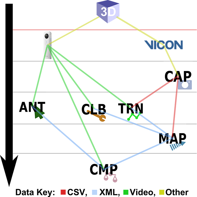
Figure 1: Overview of the UniSA omnidirectional data set acquisition and automatic annotation. RICOH THETA m15 image (2D) and VICON positional (3D) centroid data were captured (CAP) in the lab. Point correspondences from chessboard calibration images (CLB) and training data from a VICON calibration wand (TRN) were used to compute the intrinsic camera parameters and its pose, respectively. This enabled the projection (MAP) of 3D target object positions measured by the VICON system to 2D image centroids. These annotations may then be used to evaluate (CMP) the performance of a human annotator or visual tracking system (ANT).

Current benchmarks for multi-object visual tracking and recognition (e.g. [2, 3, 4, 5]) have employed human annotators together with semi-automatic image annotation tools to supply ground truth data, which introduces unknown bias into the performance evaluation of machine vision systems [6]. Unlike this previous work, our data set provides ground truth image annotations that have been automatically mapped from 3D object positions measured by a VICON motion capture system, using a process illustrated in Figure 1. This approach avoids ad hoc error prone human annotation and allows the systematic error on the ground truth image annotations to be estimated.

Omnidirectional vision systems have found application in autonomous driving technology [7], traffic surveillance [8] and threat warning [9], where large fields of view may be coupled with machine vision to provide complete situational awareness of surroundings. Such systems can consist of multiple sensors whose images are fused together [10]. Alternatively, they may employ dioptric (fisheye lenses) or catadioptric (hyperbolic/parabolic/spherical mirrors) optics to provide a spherical field of view. Omnidirectional cameras enable object tracking and recognition over a wider area and longer length of time than can be achieved using standard perspective projection cameras, but this typically comes at the expense of image resolution and additional distortion. The UniSA omnidirectional data set aims to promote research in this area by enabling the training and evaluation of omnidirectional vision algorithms for the detection, tracking and fine-grained recognition of multiple generic objects.

In this paper we describe the UniSA omnidirectional data set, which is made available publicly through our website. The work presented consists of the following key contributions:

• A novel approach to ground truth image annotation for visual tracking and object recognition data sets that is automated and avoids the need for human annotators.

• A set of $43$ omnidirectional videos of moving and stationary target objects in a variety of scenarios, which include occlusions, lighting changes, clutter and fog.

• A corresponding set of ground truth centroid positions for each object unique identifier (ID), which have been mapped into the image from precisely measured 3D world coordinates.

• The publicly available software environment, which provides a suite of tools for data capture, camera calibration, ground truth mapping and comparison with results obtained by human annotators or visual tracking systems.

• Raw calibration and 3D position data to which the software tools may be applied to re-calibrate the camera and/or re-map the ground truth annotations, respectively.

The rest of this paper is organized as follows. Section II presents a review of key recent developments in omnidirectional vision research and relevant benchmark data sets. Section III describes the experimental setup, methodology and the resulting data products of the UniSA omnidirectional data set. Section IV outlines how these data may be used to evaluate omnidirectional vision systems. Finally, section V concludes the paper, outlining directions of future work to advance the data set.

II Related Work

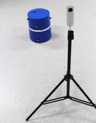
Figure 2: RICOH THETA m15 omnidirectional camera mounted on a tripod and a target object in the background. Each target consists of a MechBot covered by a container whose surface is sparsely covered with 9 mm diameter markers, which define a unique constellation that can be tracked by the lab’s VICON system.

Benchmarks for multi-object visual tracking typically exercise only a specific type of object, such as pedestrians in the MOT Challenge [2, 3] or vehicles in UA–DETRAC [4], to which highly tuned object detectors can be applied. By contrast, the DARPA Neovision2 benchmark [5] captured video of multiple object types to assist the development of detection and recognition algorithms. A subset of its ground truth data has also been extended to include unique object IDs for tracking evaluation [11]. In addition, the KITTI [12] and ImageNet VID [13] benchmarks are designed for multi-class, multi-object detection and tracking. Unlike the aforementioned data sets, ours captures both stationary and moving targets that are generic objects of rigid shape. Moreover, our videos were recorded using an omnidirectional camera, as shown in Figure 2.

Depending on the specific geometry of the omnidirectional camera optics, the resultant projection can lead to severe image distortion. This presents a challenge for standard image processing techniques and a number of dedicated solutions have been proposed in the context of structure from motion [1, 14], 3D reconstruction [15], visual odometry [16], object detection [17] and tracking [18, 8] using omnidirectional imagery.

Research in these areas has also led to the release of several task–specific omnidirectional data sets focusing on structure from motion [19, 20], visual odometry [7, 21], human detection [22] and tracking [23, 24], and vehicle detection [25] and recognition [26, 27]. We note that the ground truth image annotations provided with each of these data sets are reliant on human input, with the exception of AMUSE [7]. Similar to our approach, the authors provide raw sensor recordings of the environment, however, unlike our data set, they leave it to the end user to determine the ground truths.

The KITTI benchmark [12] consists of video captured using two stereo camera rigs (grayscale and color) that are combined with localization sensor data for the recording platform and 3D point cloud data from a Velodyne laser scanner. The aim is to evaluate computer vision tasks required in autonomous driving, which include stereo estimation, optical flow, visual odometry and 3D object tracking. While not omnidirectional, this data set is conceptually similar to ours in terms of its ground truth data, which is mapped into the image [28]. We note, however, that their ground truth 3D bounding box tracklets are still assigned to dynamic objects by human annotators, and this is a key point of difference to our approach, which removes humans from the ground truth annotation process.

III UniSA Omnidirectional Data Set

The UniSA omnidirectional data set consists of $43$ spherical videos and corresponding ground truth object positions measured in 3D world coordinates by a VICON system. These raw data were captured over four sessions in the UniSA Mechatronics Laboratory. This section describes the experimental setup and software tools used to implement the process illustrated by Figure 1, together with the resulting data set.

III-A Experimental Setup

Videos were recorded with a RICOH THETA m15 spherical camera whose dual fisheye lens system provides a spherical ($4\pi$ steradian) field of view. The camera remained stationary during each recording session, being mounted on a tripod as shown in Figure 2 and having recordings triggered via a smart phone application. Raw videos were recorded at $15$ frames per second in MOV format with MPEG-4 AVC/H.264 compression. Each HD ($1920\times 1080$) resolution image frame contains two fisheye images that correspond to opposite hemispheres, which are treated separately as side-by-side $960\times 1080$ pixel sized images [29].

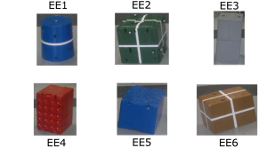
Figure 3: The six target objects present in the UniSA omnidirectional data set: blue tub EE1, green box EE2, tall gray box EE3, tall large red box EE4, long blue box EE5 and small brown box EE6.

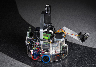
Figure 4: Mechatronic Robots (MechBots) are used to move each target and are controlled using PlayStation 3 controllers.

Up to six targets were captured as part of the data set and these are shown in Figure 3, with their dimensions listed in Table I. Remote controlled round ground-based robots of diameter $250$ mm with two drive wheels and two jockey wheels (MechBots), such as that seen in Figure 4, were placed under each container to enable target motion. The position of each object was tracked with sub-mm accuracy by a VICON system recording at around $40$ Hz. The 3D tracking is based on the unique constellation of markers on each object that is observed by eight Bonita B10 cameras, and this is illustrated in Figure 5 for one of the camera views.

	dimensions
EE1	diameter $=85$ mm height $=315$ mm
EE2	$330\times 330\times 330$ mm
EE3	$280\times 280\times 555$ mm
EE4	$380\times 335\times 490$ mm
EE5	$330\times 495\times 280$ mm
EE6	$290\times 385\times 270$ mm

TABLE I: Target object dimensions

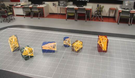
Figure 5: VICON target objects (yellow constellations defined by markers) as displayed using the VICON motion capture system software and superimposed on an image of the scene.

Our Python software environment includes the VICON capture tool (CAP), which interfaced with the VICON system to record the raw ground truth data. For each target object, a CSV file was written containing the object position $(X,Y,Z)$ and orientation (pitch, roll, yaw) in VICON world coordinates together with the number of markers detected by the system, the VICON frame number and synchronization information.

III-B Data Synchronization

A custom built synchronization circuit was connected via serial port to the data acquisition PC and used to trigger a camera flash near the start and end of each video recording. This allowed the two flash events to be logged within a designated synchronization field of each raw CSV file produced by the capture tool. The two video frames containing each flash were subsequently specified manually and these correspondences were used on the fly by the toolkit to line up in time each video frame with its nearest VICON frame.

III-C Camera Calibration

Our camera calibration and pose estimation procedures both leverage OpenCV library implementations of [30] and [31] through its Python API to calculate the intrinsic and extrinsic camera parameters.

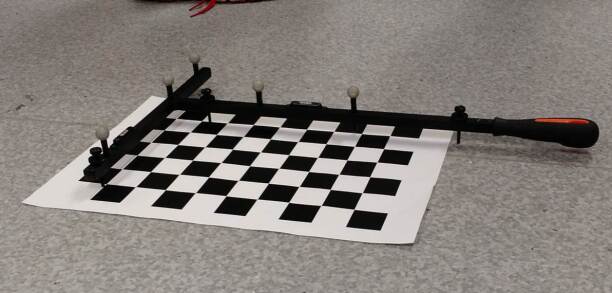
(a)

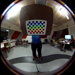
(b)

Figure 6: (a) Objects used for camera calibration: $9\times 6$ chessboard pattern with 35.3 mm side squares and VICON calibration wand with five markers. (b) RICOH THETA m15 single lens view of the chessboard pattern, showing the image training points extracted by OpenCV automatic corner detection.

III-C1 Intrinsic Parameters

A perspective projection model was computed separately for each lens using the camera calibration tool (CLB). This used the corner points extracted from multiple views of a chessboard pattern as input, and these images are provided as part of the data set, with one example shown in Figure 6. The parameters include the focal lengths ($f_{x}$ and $f_{y}$) and principal point coordinates ($c_{x}$ and $c_{y}$), which are in pixel units and serve as the elements of the camera matrix A in the following transform [32]:

$$\begin{gathered}s\;\textbf{m}=\textbf{A}[\textbf{R}|\textbf{t}]\textbf{M}\\ s\begin{bmatrix}u\\ v\\ 1\end{bmatrix}=\begin{bmatrix}f_{x}&0&c_{x}\\ 0&f_{y}&c_{y}\\ 0&0&1\end{bmatrix}\begin{bmatrix}r_{11}&r_{12}&r_{13}&t_{1}\\ r_{21}&r_{22}&r_{23}&t_{2}\\ r_{31}&r_{32}&r_{33}&t_{3}\end{bmatrix}\begin{bmatrix}X\\ Y\\ Z\\ 1\end{bmatrix}\end{gathered}$$ (1)

Ignoring distortion, Eqn. 1 describes the projection of a corner position M in world coordinates defined by the chessboard plane (such that $Z=0$) to its corresponding image point m with pixel coordinates ($u,v$), where $s$ is a scale factor. The rotation matrix R and translation vector t relate the (fixed) camera pose to the coordinate system defined by a given chessboard orientation.

To handle real cameras, the intrinsic parameters also include distortion coefficients, which are used to model the radial ($k_{1},...,k_{6}$) and tangential ($p_{1},p_{2}$) image distortion in Eqn. 2 below. In order to handle the strong radial distortion induced by the fisheye projection, we applied the OpenCV rational model, which activates three additional radial coefficients: $k_{3},k_{4},k_{6}$. This provides a denominator term Eqn. 2, which would otherwise be $1$ under default settings. Expanding out Eqn. 1 to an equivalent series of expressions, this distortion model is incorporated into the transform as follows [32]:

$$\begin{gathered}\begin{pmatrix}x\\ y\\ z\end{pmatrix}=\textbf{R}\begin{pmatrix}X\\ Y\\ Z\end{pmatrix}+\textbf{t}\\ x^{\prime}=x/z\\ y^{\prime}=y/z\\ x^{\prime\prime}=x^{\prime}\frac{1+k_{1}r^{2}+k_{2}r^{4}+k_{3}r^{6}}{1+k_{4}r^{2}+k_{5}r^{4}+k_{6}r^{6}}\\ +2p_{1}x^{\prime}y^{\prime}+p_{2}(r^{2}+2x^{\prime 2})\\ y^{\prime\prime}=y^{\prime}\frac{1+k_{1}r^{2}+k_{2}r^{4}+k_{3}r^{6}}{1+k_{4}r^{2}+k_{5}r^{4}+k_{6}r^{6}}\\ +p_{1}(r^{2}+2y^{\prime 2})+2p_{2}x^{\prime}y^{\prime}\\ \text{where}\quad r^{2}=x^{\prime 2}+y^{\prime 2}\\ u=f_{x}\times x^{\prime\prime}+c_{x}\\ v=f_{y}\times y^{\prime\prime}+c_{y}\end{gathered}$$ (2)

III-C2 Extrinsic Parameters

The camera pose estimation must be performed separately for each lens and for each of the four data capture sessions. The procedure relies on a set of 2D image and 3D object training point correspondences, where each point is the marker at the ‘T-junction’ of the VICON calibration wand seen in Figure 6. Training sets for each lens were built by performing the data acquisition with the wand as the target to collect object points. A human operator then used the training tool (TRN) to annotate a number of image points through mouse clicks on the marker at different frames, as the wand moved throughout the room. While a minimum of $4$ training points are required for each lens, in excess of $20$ were used in practice. These were output by the training tool in XML file format and are provided as part of the data set.

Given the appropriate training set and intrinsic parameters, the camera pose is estimated on the fly for each lens by the mapping tool (MAP). The training point correspondences and fixed intrinsic parameters are passed to the OpenCV function solvePnP, where the camera pose is first estimated by the Direct Linear Transform method and then optimized through an iterative procedure based on the Levenberg-Marquardt algorithm. This finds the rotation matrix R and translation vector t necessary to describe the transformation from the VICON world coordinate system to a camera world coordinate system.

III-D Mapping Ground Truth Positions

Once the camera was calibrated and a pose estimation training set had been built, the VICON coordinates of new target objects were mapped automatically in order to generate ground truth data for every video.

III-D1 Switching between the lenses

In order to perform the mapping, the appropriate lens must first be selected. To this end, the mapping tool applies extrinsic parameters of each lens to each VICON position $(X,Y,Z)$ in order to convert the object position to camera world coordinates for that particular lens:

$$\begin{pmatrix}x\\ y\\ z\end{pmatrix}=\textbf{R}\begin{pmatrix}X\\ Y\\ Z\end{pmatrix}+\textbf{t}\\$$ (3)

By converting this into spherical coordinates:

$$\begin{gathered}r=\sqrt{x^{2}+y^{2}+z^{2}}\\ \theta=\arccos\frac{z}{\sqrt{x^{2}+y^{2}+z^{2}}}\\ \phi=\arctan\frac{y}{x}\end{gathered}$$ (4)

the zenith angle $\theta$ is used to determine in which of the hemispheres the object is located, and hence which set of parameters should be used to perform the mapping.

III-D2 Mapping 3D positions to 2D centroids

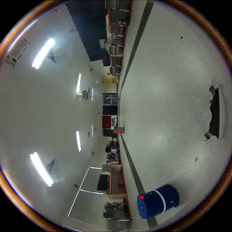
(a)

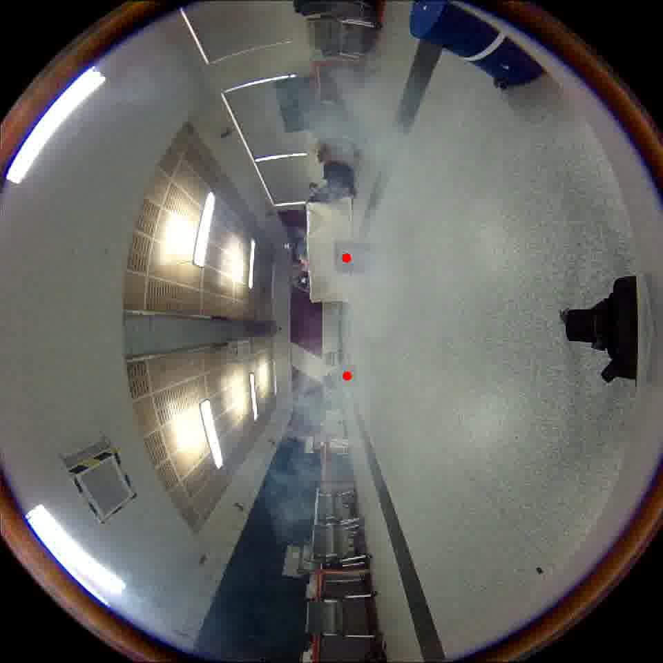
(b)

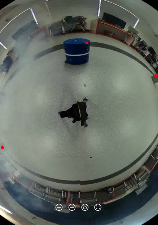
(c)

Figure 7: Mapped ground truth annotations (red points) in video ‘Set 33’ of session 4 displayed in the (a) left and (b) right side images of a video frame, which can be stitched into an equirectangular image and displayed in (c) using the RICOH THETA spherical viewer [33]. Of the four target objects (EE1, EE3, EE4, EE5) in this frame, two are obscured by fog from a fog machine.

The projection into the image of object positions measured by the VICON system was performed using the mapping tool according to Eqn. 2, where the extrinsic parameters R and t were computed from the wand training points. Table II presents a overview of the the $43$ mapped videos contained in the UniSA omnidirectional data set. Figure 7 illustrates some sample results in two fisheye images. Furthermore, these can be stitched and converted into an equirectangular image by using the RICOH THETA Spherical Viewer [33], which displays it on the sphere.

Name	Video	Frames	Start	End	Targets	Scenario Notes
Session 1 Set 1	R0010216	325	36	362	EE2	Single target, still
Session 1 Set 2	R0010218	324	37	362	EE2	Single target, moving from off-screen
Session 1 Set 3	R0010219	324	31	356	EE2	Single target, moving on-screen, across two lens
Session 1 Set 4	R0010220	341	14	356	EE2	Single target, moving on-screen, single lens
Session 1 Set 5	R0010221	324	37	362	EE2	Single target, full occlusion
Session 1 Set 6	R0010222	334	27	354	EE2	Single target, partial occlusion
Session 1 Set 7	R0010224	324	30	355	EE2	Single target, lighting variation
Session 1 Set 8	R0010226	335	34	370	EE2, EE5	2 targets, separate lens
Session 1 Set 9	R0010227	324	36	361	EE2, EE5	2 targets, same lens, no occlusion
Session 1 Set 10	R0010228	333	28	362	EE2, EE5	2 targets, same lens, partial occlusion
Session 1 Set 11	R0010229	326	35	362	EE2, EE5	2 targets, same lens, multi occlusion
Session 1 Set 12	R0010230	329	36	366	EE2, EE4, EE5	3 targets, 1 stationary, multi occlusion with lighting variations
Session 1 Set 13	R0010232	342	23	348	EE2, EE3, EE4, EE5	4 targets, 2 stationary, separate lenses, partial occlusion
Session 1 Set 14	R0010233	325	34	360	EE2, EE3, EE4, EE5	4 targets, 2 stationary, separate lenses, full occlusion
Session 2 Set 15	R0010238	326	32	359	EE1, EE2, EE4, EE5	4 targets moving in sectors, no crossing lens & occlusions
Session 3 Set 16	R0010242	337	42	380	EE1, EE2, EE3, EE4, EE5, EE6	6 targets, no occlusions, 1 cross lens
Session 3 Set 17	R0010243	341	34	376	EE1, EE2, EE3, EE4, EE5, EE6	6 targets, varied occlusions, 1 cross lens
Session 3 Set 18	R0010244	349	41	391	EE1, EE2, EE3, EE4, EE5, EE6	5 moving targets, 1 stationary target, rotation, occlusions
Session 3 Set 19	R0010245	1260	26	1287	EE1, EE2, EE3, EE4, EE5, EE6	6 targets, long set, loop around blue, occlusions
Session 3 Set 20	R0010246	1349	38	1388	EE1, EE2, EE3, EE4, EE5, EE6	6 targets, long set, lots of clutter with chairs
Session 3 Set 21	R0010247					Reference frame, no targets
Session 3 Set 22	R0010248	1256	40	1297	EE1, EE2, EE4, EE5, EE6	5 targets, long set, reveal from off-scene
Session 3 Set 23	R0010249	1257	43	1301	EE1, EE2, EE4, EE5, EE6	5 targets, long set, chasing humanoid object, occlusions
Session 3 Set 24	R0010250	324	48	373	EE1, EE2, EE4, EE5, EE6	5 targets, moving before, stop mid-scene with clutter
Session 3 Set 25	R0010251	324	36	361	EE1, EE2, EE4, EE5, EE6	5 targets, spinning on spot
Session 3 Set 26	R0010252	319	41	367	EE1, EE2, EE3, EE4, EE5, EE6	5 targets, spinning counter
Session 3 Set 27	R0010253	324	46	371	EE1, EE2, EE4, EE5, EE6	5 targets, with drivers as clutter
Session 3 Set 28	R0010254	324	41	366	EE1, EE2, EE4, EE5, EE6	5 targets, lighting changes on backside
Session 3 Set 29	R0010255	328	35	364	EE1, EE2, EE4, EE5, EE6	5 targets, lighting changes on buttonside
Session 3 Set 30	R0010256	327	42	370	EE1, EE2, EE4, EE5, EE6	5 targets, lighting changes on buttonside
Session 4 Set 31	R0010259					Reference frame, no targets
Session 4 Set 32	R0010261	335	35	371	EE1, EE3, EE4, EE5	4 targets, a little fog
Session 4 Set 33	R0010262	324	40	365	EE1, EE3, EE4, EE5	4 targets, a lot of fog
Session 4 Set 34	R0010263	338	41	365	EE1, EE3, EE4, EE5	4 targets, misty fog with total lighting changes
Session 4 Set 35	R0010264	332	44	377	EE1, EE3, EE4, EE5	4 targets, fog pointed at camera, single side lighting changes
Session 4 Set 36	R0010265	346	35	382	EE1, EE3, EE4, EE5	4 targets, no fog, complete dark start
Session 4 Set 37	R0010266	339	42	382	EE1, EE3, EE4, EE5	4 targets, fog with spinning
Session 4 Set 38	R0010267	325	42	368	EE1, EE3, EE4, EE5	4 targets, fog with anti-clockwise rotation
Session 4 Set 39	R0010268	328	35	372	EE1, EE3, EE4, EE5	4 targets, no fog, all robots occlude behind a single robot
Session 4 Set 40	R0010269	328	46	375	EE1, EE3, EE4, EE5	4 targets, no fog, all robots occlude behind a single robot
Session 4 Set 41	R0010272	325	34	360	EE1, EE3, EE4, EE5	4 targets, random stuff
Session 4 Set 42	R0010273	324	37	362	EE1, EE3, EE4, EE5	3 moving targets, 1 stationary, occlusion, bumps
Session 4 Set 43	R0010274	324	39	364	EE1, EE3, EE4, EE5	3 moving targets, 1 stationary, occlusion bumps

TABLE II: Overview of the UniSA omnidirectional data set

Although the annotations tend to look reasonable by eye, mapping errors do occur in some cases. Figure 7a shows one such case, where the annotation of the nearest object (EE1) is not well centered on the object. This is likely due to poor mapping near the edge of the lens field of view, where the distortion given by the fisheye projection is strong and not well modeled (see below). In section V we outline a future direction for improving our current calibration method, which may overcome this type of problem. Here on the other hand we seek to quantify the systematic error on the ground truth annotations.

III-D3 Expected Error

In order to estimate the systematic error on mapped centroids, the Compare Trainer utility tool compared re-projected VICON calibration wand marker points with their corresponding image training points. Using the wand for this is necessary because it is known a priori precisely to which 3D position (marker) the measured VICON coordinates belong. Figure 8 provides an example of one such comparison, which captures errors induced by imperfections in both the camera model (including distortion) and the pose estimation. The Euclidean distances between the training and re-projection points were measured using all training examples for each of the two lenses and every data capture session. Their spatial distribution across each image, shown in Figure 9, suggests that mapped points near the edge of the field of view are subject to some of the largest systematic errors, although examples of good mappings are also found in the outer regions. Tables III, IV, V and  VI summarize the re-projection error in terms of the sample mean and standard deviation $\sigma$, while the number of training points used is also listed.

	mean (pixels)	$\sigma$ (pixels)	Points
Left lens	8.22	3.79	30
Right lens	5.53	3.23	21

TABLE III: Re-projection error in Session 1.

	mean (pixels)	$\sigma$ (pixels)	Points
Left lens	7.23	4.06	72
Right lens	5.80	4.21	56

TABLE IV: Re-projection error in Session 2.

	mean (pixels)	$\sigma$ (pixels)	Points
Left lens	6.73	3.21	48
Right lens	5.88	3.41	30

TABLE V: Re-projection error in Session 3.

	mean (pixels)	$\sigma$ (pixels)	Points
Left lens	6.82	4.31	36
Right lens	5.17	2.52	22

TABLE VI: Re-projection error in Session 4.

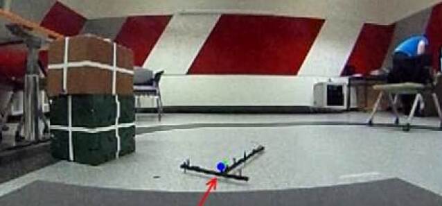
Figure 8: The red arrow indicates a mapped image point (green) and the corresponding training point (blue) on the calibration wand marker. The green point has been obtained by projecting the measured world coordinates of the marker using the mapping tool (MAP). The training point (blue) was labeled by a human using the training tool (TRN) and contributed to the determination of the extrinsic parameters used in the mapping. The Euclidean distance between the two points measures the re-projection error given by the mapping, which in this example is $2.78$ pixels.

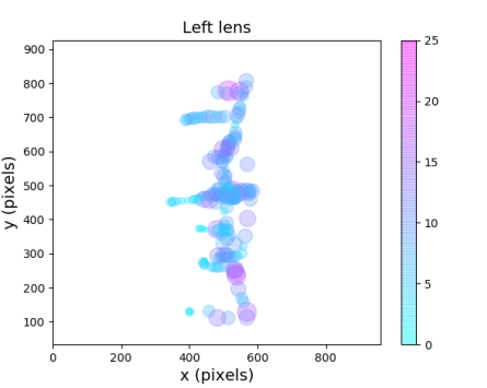
(a)

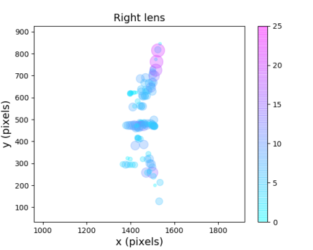
(b)

Figure 9: Wand re-projection errors in all sessions shown at their image training points in the (a) left and (b) right lens images, where the axes are oriented as those in Figures 7a and 7b, respectively. The re-projection error is indicated by the marker color in units of pixels, while the marker size also scales linearly with this value, such that larger markers indicate larger error.

IV Performance Evaluation Framework

This section outlines the way in which the performance of visual tracking systems or human annotators may be compared and evaluated against the automatic ground truth annotations produced for the UniSA omnidirectional data set.

IV-A Wizard GUI

A graphical user interface (GUI) called Wizard exists to guide users through the process summarized by Figure 1. Rather than running tools from the command line, users can opt to replicate the work flows described in previous section using the Wizard, starting with the camera calibration and/or the trainer tools, or alternatively, by using the mapped ground truths provided. Furthermore, Wizard sessions save metadata in an XML header file, which maintains a record of input files and allows a zipped data set to be re-loaded.

IV-B Ground Truth Data Format

If re-calibration and re-mapping are not required, the user may simply compare (CMP) our ground truth data, which are the mapped image annotations, against results from their vision system. This requires both inputs to the comparison tool to have a common format, which is described below.

⬇

<dataset>

<frameInformation>

<frame number=”1” />

<object name=”EE1” lens=”Backside” id=”01”>

<boxinfo y=”488” x=”499” width=”63” height=”74”/>

<centroid y=”525” x=”530”/>

<visibility visible=”5” visibleMax=”5”/>

</object>

<object name=”EE2” lens=”Buttonside” id=”02”>

<boxinfo y=”406” x=”1465” width=”83” height=”104”/>

<centroid y=”458” x=”1506”/>

<visibility visible=”5” visibleMax=”5”/>

</object>

</frameInformation>

</dataset>

The example above illustrates the ground truth annotation format. Each object name is associated with a unique ID. The choice of lens is defined by which half of the $1920\times 1080$ pixel frame the centroid is located: Backside/Buttonside refers to the left/right image in the frame. The visbility tag indicates the quality of the VICON tracking and this is used by the comparison tool to decide whether ground truth data is available for that object and at that frame. A boxinfo attribute is provided as a place holder and currently has rather arbitrary values that prescribe the corner and dimension of a rectangular bounding box centred on the centroid. The reason behind this is that only the projected position (and not the projected shape) is available. In future releases we intend to refine the bounding boxes and automatically scale them with the distance to the object.

IV-C Evaluation of vision systems

The evaluation tool (CMP) provides a simple frame-by-frame calculation of the the Euclidean distance between each ground truth annotation and the position of that object output by vision system. Here we provide a semi-automated annotation tool (ANT) based on [34] as a demonstrator for a vision system that outputs its results in the required format. Comparisons are made for ground truth and system objects with the same name and on the same lens. One of the requirements for the vision system is therefore to assign the correct ID to the each object, in every frame and multi-object trackers can perform this task. The comparison tool output includes frame-by-frame display of the Euclidean error, which can be toggled between each ground truth object present in the video.

V Conclusion

This paper has presented a novel approach to automatic ground truth annotation for multi-object visual tracking. To our best knowledge, the idea of automatically mapping 3D ground truth positions into the image has not been implemented without input from human annotators in public benchmarks for visual tracking. We use our approach to create the UniSA omnidirectional data set, which provides the research community with $43$ spherical annotated videos of moving and stationary targets under a variety of challenging scenarios. We also supply the raw world coordinate data and raw calibration data.

Based on the video and ground truth data provided, the UniSA omnidirectional data set may be used to train and evaluate algorithms for the object detection, tracking and fine-grained recognition of multiple objects. In the latter case, the omnidirectional vision system could, for example, be required to detect all target objects while ignoring all others (e.g. people and furniture) considered to be clutter, and then reconize a particular object type (e.g. only the elongated containers).

A key aspect of this data set is that the camera can be re-calibrated (e.g. with a refined camera model) and the ground truth annotations can be subsequently re-mapped. To this end, we plan to investigate the application of the spherical OcamCalib Toolbox for Matlab [35] to our data. An outstading issue is that unlike the toolbox by Bouguet [30], which is implemented in OpenCV to handle 3D calibration structures, OCamCalib only solves the extrinsic parameters of planar homographies, and so can not be directly applied to find our extrinsic parameters based on calibration wand points. Nevertheless, we expect that any future release of our data set will involve the application of its spherical camera model to handle the perspective projection of the dual fisheye lens camera.

References

- [1] C. Demonceaux and P. Vasseur, “Omnidirectional image processing using geodesic metric,” in 16th IEEE International Conference on Image Processing (ICIP). IEEE, 2009, pp. 221–224.
- [2] L. Leal-Taixé, A. Milan, I. Reid, S. Roth, and K. Schindler, “MOTChallenge 2015: Towards a benchmark for multi-target tracking,” arXiv:1504.01942 [cs], Apr. 2015, arXiv: 1504.01942. [Online]. Available: http://arxiv.org/abs/1504.01942
- [3] A. Milan, L. Leal-Taixé, I. Reid, S. Roth, and K. Schindler, “MOT16: A benchmark for multi-object tracking,” arXiv:1603.00831 [cs], Mar. 2016, arXiv: 1603.00831. [Online]. Available: http://arxiv.org/abs/1603.00831
- [4] L. Wen, D. Du, Z. Cai, Z. Lei, M. Chang, H. Qi, J. Lim, M.-H. Yang, and S. Lyu, “Detrac: A new benchmark and protocol for multi-object tracking,” arXiv preprint arXiv:1511.04136, 2015.
- [5] R. Kasturi, D. B. Goldgof, R. Ekambaram, G. Pratt, E. Krotkov, D. D. Hackett, Y. Ran, Q. Zheng, R. Sharma, M. Anderson et al., “Performance evaluation of neuromorphic-vision object recognition algorithms,” in 22nd International Conference on Pattern Recognition (ICPR). IEEE, 2014, pp. 2401–2406.
- [6] A. Milan, K. Schindler, and S. Roth, “Challenges of ground truth evaluation of multi-target tracking,” in Proceedings of the IEEE Conference on Computer Vision and Pattern Recognition Workshops, 2013, pp. 735–742.
- [7] P. Koschorrek, T. Piccini, P. Öberg, M. Felsberg, L. Nielsen, and R. Mester, “A multi-sensor traffic scene dataset with omnidirectional video,” in Ground Truth - What is a good dataset? CVPR Workshop 2013, 2013.
- [8] W. Wang, T. Gee, J. Price, and H. Qi, “Real time multi-vehicle tracking and counting at intersections from a fisheye camera,” in IEEE Winter Conference on Applications of Computer Vision (WACV). IEEE, 2015, pp. 17–24.
- [9] T. C. Brusgard, “Distributed aperture infrared sensor systems,” in Proc. SPIE, vol. 3698, 1999, pp. 58–66.
- [10] X. Peng, M. Bennamoun, Q. Wang, Q. Ma, and Z. Xu, “A low-cost implementation of a 360° vision distributed aperture system,” IEEE Transactions on Circuits and Systems for Video Technology, vol. 25, no. 2, pp. 225–238, 2015.
- [11] A. Chakraborty, V. Stamatescu, S. C. Wong, G. Wigley, and D. Kearney, “A data set for evaluating the performance of multi-class multi-object video tracking,” in SPIE Defense+Security. International Society for Optics and Photonics, 2017, pp. 102 020G–102 020G.
- [12] A. Geiger, P. Lenz, and R. Urtasun, “Are we ready for Autonomous Driving? the KITTI Vision Benchmark Suite,” in Conference on Computer Vision and Pattern Recognition (CVPR), 2012.
- [13] O. Russakovsky, J. Deng, H. Su, J. Krause, S. Satheesh, S. Ma, Z. Huang, A. Karpathy, A. Khosla, M. Bernstein et al., “ImageNet Large Scale Visual Recognition Challenge,” International Journal of Computer Vision, vol. 115, no. 3, pp. 211–252, 2015.
- [14] H. Taira, Y. Inoue, A. Torii, and M. Okutomi, “Robust feature matching for distorted projection by spherical cameras,” IPSJ Transactions on Computer Vision and Applications, vol. 7, pp. 84–88, 2015.
- [15] C. Ma, L. Shi, H. Huang, and M. Yan, “3d reconstruction from full-view fisheye camera,” arXiv preprint arXiv:1506.06273, 2015.
- [16] H. Hadj-Abdelkader, E. Malis, and P. Rives, “Spherical image processing for accurate visual odometry with omnidirectional cameras,” in The 8th Workshop on Omnidirectional Vision, Camera Networks and Non-classical Cameras-OMNIVIS, 2008.
- [17] I. Cinaroglu and Y. Bastanlar, “A direct approach for object detection with catadioptric omnidirectional cameras.” Signal, Image and Video Processing, vol. 10, no. 2, pp. 413–420, 2016.
- [18] A. Salazar-Garibay, E. Malis, and C. Mei, “Visual tracking of planes with an uncalibrated central catadioptric camera,” in Intelligent Robots and Systems, 2009. IROS 2009. IEEE/RSJ International Conference on. IEEE, 2009, pp. 2999–3004.
- [19] Y. Bastanlar, A. Temizel, Y. Yardimci, and P. Sturm, “Multi-view structure-from-motion for hybrid camera scenarios,” Image and Vision Computing, vol. 30, no. 8, pp. 557–572, 2012.
- [20] A. R. Zamir and M. Shah, “Image geo–localization based on multiple nearest neighbor feature matching using generalized graphs,” IEEE transactions on pattern analysis and machine intelligence, vol. 36, no. 8, pp. 1546–1558, 2014.
- [21] Z. Zhang, H. Rebecq, C. Forster, and D. Scaramuzza, “Benefit of large field-of-view cameras for visual odometry,” in IEEE International Conference on Robotics and Automation (ICRA). IEEE, 2016, pp. 801–808.
- [22] I. Cinaroglu and Y. Bastanlar, “A direct approach for human detection with catadioptric omnidirectional cameras,” in Signal Processing and Communications Applications Conference (SIU), 2014 22nd. IEEE, 2014, pp. 2275–2279.
- [23] B. E. Demiröz, İ. Ari, O. Eroğlu, A. A. Salah, and L. Akarun, “Feature-based tracking on a multi-omnidirectional camera dataset,” in 5th International Symposium on Communications Control and Signal Processing (ISCCSP). IEEE, 2012, pp. 1–5.
- [24] GTI-UPM. (2016) PIROPO Database. [Online]. Available: https://sites.google.com/site/piropodatabase/home
- [25] H. C. Karaimer and Y. Bactanlar, “Car detection with omnidirectional cameras using haar-like features and cascaded boosting,” in Signal Processing and Communications Applications Conference (SIU), 2014 22nd. IEEE, 2014, pp. 301–304.
- [26] H. C. Karaimer and Y. Bastanlar, “Detection and classification of vehicles from omnidirectional videos using temporal average of silhouettes,” in 10th International Conference on Computer Vision Theory and Applications, 2015, pp. 197–204.
- [27] İ. Barış, “Classification and tracking of vehicles with hybrid camera systems,” Master’s thesis, İzmir Institute of Technology, 2016.
- [28] A. Geiger, P. Lenz, C. Stiller, and R. Urtasun, “Vision meets robotics: The KITTI dataset,” The International Journal of Robotics Research, vol. 32, no. 11, pp. 1231–1237, 2013.
- [29] RICOH THETA. (2015) Camera Specifications. [Online]. Available: https://theta360.com/en/about/theta/m15.html
- [30] J.-Y. Bouguet. (2015) Camera calibration toolbox for matlab. [Online]. Available: http://www.vision.caltech.edu/bouguetj/calib_doc/
- [31] Z. Zhang, “A flexible new technique for camera calibration,” IEEE Transactions on Pattern Analysis and Machine Intelligence, vol. 22, no. 11, pp. 1330–1334, 2000.
- [32] OpenCV. (2015) Camera Calibration Documentation. [Online]. Available: http://docs.opencv.org/3.0.0/d9/d0c/group__calib3d.html
- [33] RICOH THETA. (2015) Computer Application. [Online]. Available: https://theta360.com/en/support/download/
- [34] İ. Arı and Y. Açıköz. (2011) Fast Image Annotation with Pinotator. [Online]. Available: http://code.google.com/p/pilab-annotator/
- [35] D. Scaramuzza, A. Martinelli, and R. Siegwart, “A flexible technique for accurate omnidirectional camera calibration and structure from motion,” in IEEE International Conference on Computer Vision Systems, 2006 ICVS’06. IEEE, 2006, pp. 45–45.