Optimal On The Fly Index Selection in Polynomial Time

Abstract

The index selection problem (ISP) is an important problem for accelerating the execution of relational queries, and it has received a lot of attention as a combinatorial knapsack problem in the past. Various solutions to this very hard problem have been provided. In contrast to existing literature, we change the underlying assumptions of the problem definition: we adapt the problem for systems that store relations in memory, and use complex specification languages, e.g., Datalog. In our framework, we decompose complex queries into primitive searches that select tuples in a relation for which an equality predicate holds. A primitive search can be accelerated by an index exhibiting a worst-case run-time complexity of log-linear time in the size of the output result of the primitive search. However, the overheads associated with maintaining indexes are very costly in terms of memory and computing time.

In this work, we present an optimal polynomial-time algorithm that finds the minimal set of indexes of a relation for a given set of primitive searches. An index may cover more than one primitive search due to the algebraic properties of the search predicate, which is a conjunction of equalities over the attributes of a relation. The index search space exhibits a complexity of $\mathcal{O}(2^{m^{m}})$ where $m$ is the number of attributes in a relation, and, hence brute-force algorithms searching for solutions in the index domain are infeasible. As a scaffolding for designing a polynomial-time algorithm, we build a partial order on search operations and use a constructive version of Dilworth’s theorem. We show a strong relationship between chains of primitive searches (forming a partial order) and indexes. We demonstrate the effectiveness and efficiency of our algorithm for an in-memory Datalog compiler that is able to process relations with billions of entries in memory.

1 Introduction

There has been a resurgence in the use of Datalog in several computer science communities including program analysis where it is used as a domain specific language (DSL) for succinctly specifying various classes of static analyses. In this setup, an input program is converted into an extensional database (EDB) and the static analysis specification is encoded as an intensional database (IDB). Such use cases, unlike traditional database queries, typically consist of hundreds of relations and hundreds of deeply nested rules [40], and result in giga-tuple sized relations [26]. Consequently, several high performance Datalog engines [26, 23, 28, 39, 3] have been employed for performing such computations. These engines use Datalog purely as a computational vehicle and use bottom-up evaluation techniques that usually involve some degree of compilation [39, 26, 33, 29]. Moreover, to further improve performance, relations are stored as indexed-organized tables in-memory, hence, enabling improved cache behaviour, lookup complexity, etc. As a result of these design characteristics, such engines require atypical index selection techniques that result in improved run-time and memory consumption while not resulting in noticeable compilation overhead.

Traditionally relational database management systems have solved the index selection problem (ISP) [36, 13, 24, 27] by variants of the $0$-$1$ knapsack problem. Such formulations implicitly solve two subproblems of query optimization, literal scheduling along side index selection. While these techniques such as [8] are well established in the relational databases literature, they are too computationally expensive for large Datalog programs and are rarely used in most Datalog engines. Too simplify this task, modern Datalog engines often require users to provide annotations to guide the engine in the choice of indices [39, 40]. Again, for large Datalog programs such approaches are very cumbersome as they put the entire optimization burden on the user, often resulting in painstaking trial and error process that results in far from optimal index performance. In this paper, we present a practical yet powerful middle ground approach: we solve the index selection optimally, while leaving join scheduling to minimal user annotations (usually on a small set of rules) or by automated means [38]. In particular, our method is ideal for compilation based engines as the index selection is performed on the fly, and results in negligible compilation time overheads while considerably boosting performance.

Our index selection approach takes into account several factors present in high-performance Datalog engines: First, in these engines, relations are not normalized and a very large number of indices may occur making the problem combinatorially intractable. Second, an index represents a whole relation and hence there is no need top capture maintenance costs in the ISP formulation as it can be assumed that all indexed relations have a uniform cost. Third, high-performance Datalog engines translate Datalog queries into intermediate representations [39, 26, 33, 29] that assume a fixed join order [39, 26] and are decomposed into a simpler relational algebra operators that operate on a single relation that we refer to primitive searches. Therefore, ISP is computed for a single relation only.

As a consequence of the new assumptions, the index selection problem is reduced to the problem of minimizing the number of indices for each relation separately. One option is to formulate the problem as a Minimum Set Cover Problem (MSCP), however, such formulations do not give us tractability, and MSCP is a too coarse as a combinatorial vehicle. On the surface it appears that finding a tractable solution is futile, considering the vast search space of all possible indices of a single relation (i.e., space of ordered attribute subsets). However, as indices need to be computed on the fly during compilation/interpretation time and by our assumption that each primitive search requires at least one index, the ISP problem can be reformulated into a covering problem, i.e., each primitive search needs an index cover. This new formulation, while more fitting to the problem at hand, also reveals deeper mathematical structures that allows us to solve the problem in polynomial-time. As a result, we are able to perform index minimization with negligible overhead and obtain significant speedups with minimal consumption.

The key to our index minimization approach is the formulation of a relationship between the space of indices and search chains. In the space of search chains we are able to leverage existing combinatorial results i.e., Dilworth’s theorem [16] that provide polynomial-time algorithms to find an optimal solutions. Using our established relationship, we are able to convert the optimal search chain solution to an optimal set of indices that we use to construct indexed joins, refered to as range nested loop joins. We further clarify our method by the motivating example below:

Example 1 (Motivating)

Assume we have a non-recursive Datalog rule that has a single ternary input relation $A(x,y,z)$ and a ternary output relation $B(x,y,z)$, where x, y and z are attributes.

$$B(r,p,q)\leftarrow A(r,p,q),A(q,\_,\_),$$

$$A(p,q,\_),A(p,\_,q),A(q,p,r).$$

This query is transformed to a nested loop join version of the query as depicted below. The details of this transformation are explained in Section 5.

$\textit{loop}_{1}$:	$\textbf{for all}\,t_{1}\in A\,\textbf{do}$
$\textit{loop}_{2}$:		$\textbf{for all}\,t_{2}\in\sigma_{x=t_{1}(z)}(A)\,\textbf{do}$
$\textit{loop}_{3}$:			$\textbf{for all}\,t_{3}\in\sigma_{x=t_{1}(y),y=t_{1}(z)}(A)\,\textbf{do}$
$\textit{loop}_{4}$:				$\textbf{for all}\,t_{4}\in\sigma_{x=t_{1}(y),z=t_{1}(z)}(A)\,\textbf{do}$
$\textit{loop}_{5}$:					$\textbf{for all}\,t_{5}\in\sigma_{x=t_{1}(z),y=t_{1}(y),z=t_{1}(x)}(A)\,\textbf{do}$
						if $t_{1}\not\in B$ then
							add $t_{1}$ to $B$
						endif
					endfor
			$\ldots$
	endfor

From the nested loop join we extract primitive searches denoted by $\sigma_{\varphi}$ where $\varphi$ is an equality predicate between attributes and contants bound by tuple values obtained further above the loop. To improve performance we use indices which we abstract as $\ell$. A naïve approach assigns each query an index which we represent by a lexicographical order, i.e., $\sqsubseteq_{\ell}$ where $\ell$ is a sequence of attributes $\ell=x\prec\dots\prec z$ that implements a lexicographical order a binary search tree. $c_{x}$ denotes a constant for attribute $x$ obtained from a tuple $t_{1}$, i.e., $t_{1}(x)$. We assign four indices to the primitive searches as shown the table below:

Query component	Primitive Search	$\ell$
$A(q,\_,\_)$	$\sigma_{x=t_{1}(z)}(A)$	$x$
$A(p,q,\_)$	$\sigma_{x=t_{1}(y),t_{1}(z)}(A)$	$x\prec y$
$A(p,\_,q)$	$\sigma_{x=t_{1}(y),z=t_{1}(z)}(A)$	$x\prec z$
$A(q,p,r)$	$\sigma_{x=t_{1}(z),y=t_{1}(y),z=t_{1}(x)}(A)$	$x\prec y\prec z$

While this assignment of indices will speed up the join computation, it is not the most optimal assignment. The research question is therefore, how can we assign indices to primitive searches in the most optimal way.

To demonstrate the practicality of our technique, we have implemented the techniques discussed in this paper in an open source, high-performance Datalog engine called Soufflé [26] that is used for large-scale static program analyses hundreds of rules and relations and processing up to giga-tuples of data.

We have performed experiments on a wide variety of program analysis specifications [40] and a diverse set of datasets that include the OpenJDK, a large industrial benchmark from Oracle. Our technique results in considerable improvements compared to several alternative indexing schemes. Our experiments suggest that our approach gives considerable run-time and memory usage improvements compared to Soufflé’s other indexing schemes. Moreover, with our technique Soufflé is able to analyze problems typically deemed too difficult for Datalog-based tools on a par with the state-of-the-art hand crafted analyzer presented in [15].

Our contributions are summarized as follows:

• We describe a join mechanism that allows for optimal index selection

• We formally define the minimal index selection problem (MOSP), including its state space.

• We introduce a novel polynomial time algorithm to solve MOSP via search chains

• We present a case study implementing MOSP in Soufflé, an open-source Datalog engine for large scale program analysis. We demonstrate the effectiveness of MOSP in Soufflé with large input instances and several real world analyses.

The paper is organized as follows: We begin with preliminary definitions in Section 2. In Section 3 we give an overview of the join computation we perform. Section 4 formally states the MOSP problem and analyses the search space of MOSP, finally leading to an optimal algorithm for solving MOSP. In Section 5 we discuss how our algorithm can potentially be integrated into databases and other query engines. In Section 6 we introduce a case study, where we implement our approach in a Datalog-based program analysis engine and evaluate our algorithm improvements observed using our technique. We highlight related work in Section 7 and draw relevant conclusions in Section 8.

2 Preliminaries

A power set of set $X$ is the set of all subsets of $X$ and is denoted by $2^{X}$. The cartesian product of two sets $X$ and $Y$ is the set of all pairs $(a,b)$ such that $a\in X$, and $b\in Y$, and is denoted by $X\times Y$. The cardinality of the Cartesian product is $|X|\cdot|Y|$. The finite n-ary cartesian product is written as $X_{1}\times\ldots\times X_{k}=\{(x_{1},\ldots,x_{k}):x_{i}\in X_{i}\}$ where elements are referred to as tuples and are defined as nested ordered pairs, i.e., $(X_{1}\times\ldots\times X_{n-1})\times X_{n}$. The permutations of set $X=\{a_{1},\ldots,a_{k}\}$ is the set of all possible sequences formed by elements of set $X$ such that each element occurs exactly once. The cardinality of $\textsf{Pm}(X)$ is given by the factorial of the cardinality of set $X$, i.e., $|\textsf{Pm}(X)|=|X|!$. We define a sequence as $a_{1}\prec a_{2}\prec\ldots\prec a_{k}$ where $\prec$ denotes a chaining of elements to form a sequence.

A relation $R\subseteq\mathbb{D}_{1}\times\ldots\times\mathbb{D}_{m}$ is a set of tuples $\{t_{1},\ldots,t_{n}\}$ where $n$ is the number of tuples in the relation, $m$ is the tuple length, and $\mathbb{D}_{i}$ are the domains of the relation. A tuple $t$ is a fixed-length vector $\langle e_{1},e_{2},...,e_{m}\rangle$ whose elements $e_{i}$ are elements of domain $\mathbb{D}_{i}$, for all $i$, $1\leq i\leq m$.

A named relation is a relation $R$ that uses attributes to refer to specific element positions. The set of attributes $A_{R}=\{x_{1},\ldots,x_{m}\}$ are $m$ distinct symbols and we write $R(x_{1},\ldots,$ $x_{m})$ to associate symbol $x_{i}$ to the $i$-th position in the tuple. The elements of tuple $t=\langle e_{1},\ldots,e_{m}\rangle$ can be accessed by access function $t(x_{i})$, which maps tuple $t$ to element $e_{i}$. E.g., given relation $R(x,y,z)$ and a tuple $t=\langle e_{1},e_{2},e_{3}\rangle\in R$, the access function is $\{t(x)\mapsto e_{1}$, $t(y)\mapsto e_{2}$ and $t(z)\mapsto e_{3}\}$.

A binary relation $R\subseteq\mathbb{D}\times\mathbb{D}$ is a set of ordered pairs. Two elements $a$ and $b$ are related in $R$ written as $aRb$, if there is a pair $(a,b)\in R$; two elements $a$ and $b$ are unrelated written as $a\not Rb$, if $(a,b)\not\in R$. A relation is reflexive, if $aRa$ for all elements $a$; symmetric, if $aRb$ implies $bRa$ for all $(a,b)\in\mathbb{D}\times\mathbb{D}$; asymmetric if $aRb$ and $bRa$ implies $a=b$, transitive if $aRb$ and $bRc$ implies $aRc$, and total if $aRb$ or $bRa$ for all $(a,b)\in\mathbb{D}\times\mathbb{D}$.

A binary relation $\leq$ is a pre-order if the relation is reflexive and transitive, a partial order if the relation is reflexive, asymmetric, and transitive, and a total order if the relation is a partial order and is total.

A lexicographical order $\sqsubseteq_{\ell}{\mathcal{D}}\times{\mathcal{D}}$ is a total order defined over the domain of a relation where ${\mathcal{D}}=\mathbb{D}_{1}\times\ldots\times\mathbb{D}_{m}$ is a finite n-ary cartesian product of the element domains, and the sequence $\ell\in L$ is formed by a subset of attributes where each attribute occurs at most once in the sequence.

3 Computing Indexed Joins

A major performance consideration in a Datalog engine is how join computations are performed. A join in traditional databases is computed by converting a Datalog rule to a primitive nested loop join. The naïve assumption is that there is no underlying tuple order inside the nested loop join resulting in linear search time complexity.

Primitive nested loop joins are defined in Fig. 1. We refer to the head atom of a Datalog clause as $R_{0}$, and each body atom as $R_{i}$ where $i>0$. We partition the sequence of body atoms at a position index $k$ into positive and negative occurrences (i.e., negative if it is negated in the body), and denote positive atoms as $R_{i}^{+}$ where $0<i\leq k$ and negative as $R_{i}^{-}$ where $i>k$, where $i$ denotes a position in the body.

In the primitive nested loop join we iterate (denoted by the for all construct) over tuples. The tuples are obtained from a filter called a primitive search defined in Def. 1 for positive relations. This comes from the implicit universal quantification in a Datalog clause. A primitive search extracts all tuples from a relation that adhere to a primitive search predicate, i.e., a predicate limited to equalities of left-hand-side attributes and right-hand-side constants bound to tuples further up the nested loop join. Negative occurring atoms are tested for emptiness w.r.t. a primitive search on already stable relations. This semantics stems from the implicit non-existence quantification on attributes of negative body literals in a Datalog rule. The most inner operation in a nested loop join projects ($\pi$) the selected tuple into the head atom if the tuple does not already exist in the relation. This existence check is performed to ensure that tuples are not inserted twice into a relation, i.e., it enforces the set constraints for relational tables. At the primitive program level, several optimizations can now be performed. For example, the join can be marked for parallelisation directives, loops which have primitive searches subsumed by another loop can be coalesced into a single loop, loops can be pushed to the most outer possible layer (know as hoisting/layering) [37].

$\textit{loop}_{1}$:	$\textbf{for all}\,t_{1}\in R^{+}_{1}\,\textbf{do}$
$\textit{loop}_{2}$:		$\textbf{for all}\,t_{2}\in\sigma_{\varphi_{2}(t_{1},t_{2})}(R^{+}_{2})$ : do
			$\ldots$
$\textit{loop}_{k}$:				for all $t_{k}\in\sigma_{\varphi_{k}(t_{1},t_{2},\ldots,t_{k})}(R^{+}_{k})$ : do
					if $\sigma_{\varphi_{k+1}(t_{1},t_{2},\ldots,t_{k})}(R^{-}_{k+1})=\emptyset$ then
					$\ldots$
						if $\sigma_{\varphi_{n}(t_{1},t_{2},\ldots,t_{k})}(R^{-}_{n})=\emptyset$ then
							if $\pi(t_{1},\ldots,t_{k})\not\in R_{0}$ then
								add $\pi(t_{1},\ldots,t_{k})$ to $R_{0}$
							endif
					$\ldots$
						endif
				endfor
			$\ldots$
		endfor
	endfor

Figure 1: Nested-Loop Join: a relational algebra query is translated by a query planner to nested loop join; each loop enumerates tuples of a relation and filters selected tuples $t_{1},\ldots,t_{k}$

Definition 1 (Primitive Search)

A primitive search has the following form:

$$\sigma_{x_{1}=v_{1},\ldots,x_{k}=v_{k}}(R_{i})\equiv\{t\in R_{i}\mid t(x_{1})=v_{1}\wedge\ldots t(x_{k})=v_{k}\}$$

where $R_{i}$ is a relation and $x_{1}=v_{1},\ldots,x_{k}=v_{k}$ is the search predicate of the relation where $x_{1},\ldots,x_{k}$ are variables (also known as attributes) of the relation and $v_{1},\ldots,v_{k}$ are either constants or values obtained from other tuple elements in relations $R_{j}$, $0<j<i$. As an alternative notation, we denote $\sigma_{{\varphi}(t_{1},\dots,t_{k})}$ where $\varphi\equiv x_{1}=v_{1},\ldots,x_{k}=v_{k}$ as the substitution of $t_{1}$ to $t_{k}$ for appropriate constants $v_{1}$ to $v_{k}$.

To improve the join computation performance we emply indices to each primitive search. Our technique rests on the assumption that all primitive searches benifit from being indexed. We refer to this assumption as the Minimal Index Assumption (MIA). the benifit of indices is that they introduce orders on tuples in relations so that tuple lookups can be performed efficiently using some notion of a balanced search tree, in which tuples can be found in logarithmic-time rather than in linear-time. To create an order among tuples in a relation, tuples must be made comparable. Since a tuple may have several elements, an order is imposed by element-wise comparison using a permutation over a subset of attributes, i.e., if the first elements produces a tie, the second elements are used and so forth. This comparison is also known as a lexicographical order. We abstract away the underlying implementation details of an index with a attribute sequence $\ell$.

$\textit{loop}_{1}$:	$\textbf{for all}\,t_{1}\in R_{1}^{+}\,\textbf{do}$
$\textit{loop}_{2}$:		$\textbf{for all}\,t_{2}\in\sigma_{\rho_{2}(\ell_{2},a_{2},b_{2})}(R_{2}^{+})\,\textbf{do}$
			$\ldots$
$\textit{loop}_{k}$:				for all $t_{k}\in\sigma_{\rho_{k}(\ell_{k},a_{k},b_{k})}(R_{k}^{+})$ do
					if $\sigma_{\rho_{k+1}(\ell_{k+1},a_{k+1},b_{k+1})}(R_{k+1}^{-})=\emptyset$ then
					$\ldots$
						if $\sigma_{\rho_{n}(\ell_{n},a_{n},b_{n})}(R_{n}^{-})=\emptyset$ then
							if $\pi(t_{1},\ldots,t_{k})\not\in R_{0}$ then
								add $\pi(t_{1},\ldots,t_{k})$ to $R_{0}$
							endif
						endif
					$\ldots$
					endif
				endfor
			$\ldots$
		endfor
	endfor

Figure 2: Loop-Nest: a relational algebra query is translated by a query planner to nested loop join; each loop enumerates tuples of a relation and filters selected tuples $t_{1},\ldots,t_{k}$ using a range tuple predicate $\rho(\ell,a,b)$. The inner most loop projects ($\pi$) selected tuples $t_{1},\ldots,t_{k}$ to a tuple for the output relation $R$. If the tuple does not exist, it will be added to the output relation.

An indexed nested loop join is refered to as a range nested loop join. Range nested loop joins are similar to primitive nested loop joins only that they are further specialized to operate on range searches. Range searches assume and index and hence assume that tuples are ordered, hence an ordered set of tuples exhibits a worst-case complexity for executing a range search in a linear-log time in the size of the output, i.e, $\mathcal{O}(|\sigma_{\rho(\ell,a,b)}|\log n)$ where $n$ is the number of tuples in a relation $R$. We define a range search in Def. 2.

Definition 2 (Range Search)

A range $\sigma_{\rho(\ell,a,b)}$ is defined for a relation $R\subseteq{\mathcal{D}}$ and its semantics is given by,

$$\sigma_{\rho(\ell,a,b)}(R)=\{t\in R\mid a\,\sqsubseteq_{\ell}\,t\wedge t\,\sqsubseteq_{\ell}\,b\}$$

where attribute sequence $\ell\in L$, lower bound $a$ and upper bound $b$ are tuples in $\mathcal{D}$, respectively.

3.1 Constructing Bounds for Range Searches

Each range search contains two symbolic bounds $a$ and $b$ in the range searches predicate as well as an index $\ell$. The primitive searches in a primitive nested loop join may not specify all attributes in their search predicate. Therefore, the construction of the lower and upper bound require care. Unspecified values need to be padded with infima and suprema values for lower and upper bounds, respectively. We define an unspecified elements for the lower/upper bound construction by an artificial constants $\triangle$. We define a bijective index mapping function $i_{k}:\{1,\ldots,m\}\rightarrow\{1,\ldots,k+1\}$ that maps the specified elements to their corresponding constant values, and the unspecified elements to $\triangle$. We further introduce an artificial value $v_{k+1}=\triangle$ for the primitive search such that for unspecified attributes the unspecified symbol $\triangle$ is used. The construction of the lower and upper bound is performed by the functions lb and ub, respectively,

$$a =\textit{lb}(v_{i_{1}},\ldots,v_{i_{m}})$$

$$b =\textit{ub}(v_{i_{1}},\ldots,v_{i_{m}})$$

that replace the unspecified $\triangle$ value to either the infimum or supremum of the domain $\mathbb{D}_{i}$, respectively. Formally, the functions are defined as $\textit{lb}(v_{1},\ldots,v_{m})=(v^{\prime}_{1},\ldots,v^{\prime}_{m})$ where

$$v^{\prime}_{i}=\begin{cases}v_{i}&\mbox{if $v_{i}\not=\triangle$}\\ \bot_{i}&\mbox{otherwise}\end{cases}$$

and $\textit{ub}(v_{1},\ldots,v_{m})=(v^{\prime}_{1},\ldots,v^{\prime}_{m})$ where

$$v^{\prime}_{i}=\begin{cases}v_{i}&\mbox{if $v_{i}\not=\triangle$}\\ \top_{i}&\mbox{otherwise}\end{cases}$$

Basically, the functions lb and ub are identity functions except for the case of unspecified values $\triangle$, which are either converted to infima of suprema of the corresponding element domain. The construction of lower and upper bounds for partial attribute searches is correct for the full attribute search, i.e., the are no unspecified values in the value.

3.2 Computing Index Sets

The next step is to compute a set of indices which are mapped to range searches predicates. For this there are several options available, including producing an index with an orderings given by the default order the attributes syntactically appear in the atom, randomized orders etc. However, when complex sets of queries (complex access patterns, variables bindings etc.) are present and when large relations are processed, constructing an optimal set of $\ell$s for range searches is crucial. As previously states this is is a variation of the classical index selection problem which we examine in more detail in Section 4 and demonstrate its performance impact in Section 6.

3.3 Range Search Cover

An important characteristic of range searches is that while exhibiting better worst-case search performance, they retain the semantics of primitive searches. We refer to this as a To establish this property we define the notion of a prefix set $\textbf{prefix}_{k}(\ell)$. The prefix set produces the first $k$ elements of an index $\ell$ over the set of attributes $\{a_{1},\ldots,a_{p}\}$ of a relation.

Definition 3 (Prefix Set)

Let $\ell=a_{{1}}\prec a_{{2}}\prec\ldots\prec a_{k}\prec a_{k+1}\prec\ldots\prec a_{{p}}$ be a lexicographical order sequence (index), the prefix set of $\ell$ is defined as:

$$\textbf{prefix}_{k}(a_{1}\prec a_{2} \prec\ldots\prec a_{k}\prec a_{k+1}\prec\ldots\prec a_{p})=$$

$$\begin{cases}\{a_{1},a_{2},\ldots,a_{k}\},\mbox{if $k\leq p$},\\ \{a_{1},a_{2},\ldots,a_{p}\},\mbox{otherwise.}\end{cases}$$

We say a range search $\sigma_{\rho(\ell,a,b)}(R)$ covers a primitive search $\sigma_{x_{1}=v_{1},\ldots,x_{k}=v_{k}}(R)$, if the $k$-th prefix of $\ell$ result in set $\{x_{1},\ldots,x_{k}\}$. Hence, an index represented by an attribute sequence $\ell$ may cover a multitude of primitive searches assuming the elements of its prefixes coincide with the attributes of the searches. Conversely, if the elements of a primitive search does not show in the elements of the $k$-th prefix of $\ell$, the primitive search cannot be covered/executed by a range search using $\ell$.

Lemma 1 (Range Search Cover)

$$\forall R\subseteq{\mathcal{D}}:\sigma_{x_{1}=v_{1},\ldots,x_{k}=v_{k}}(R)=\sigma_{\rho(\ell,a,b)}(R)$$

, $\{x_{1},\ldots,x_{k}\}=\textbf{prefix}_{k}(\ell)$, $a=\textit{lb}(v_{1},\ldots,v_{k})$, and $b=\textit{ub}(v_{1},\ldots,v_{k})$.

The correspondence can be extended for any permutation over the set $\{x_{1},\ \ldots,\ x_{k}\}$. This follows from the commutativity property of the search predicate, i.e., the actual order of the equality condition in the search primitive is irrelevant. An extension of $\ell$ with further attributes still preserves the correspondence, i.e., for all lexicographical orders $\ell=x_{1}\prec\ldots\prec x_{k}\prec x_{k+1}\prec\ldots\prec x_{k+s}$, it still holds that $\forall R\subseteq{\mathcal{D}}:\sigma_{x_{1}=v_{1},\ldots,x_{k}=v_{k}}(R)=\sigma_{\rho(\ell,a,b)}(R)$. To construct a range search for a primitive search, we need to compute the bounds and lexicographical order.

Example 2 (Motivating (Cont.))

Let us assume we have a set of primitive search predicates extracted from a query (See Section 5). The primitive search predicates are depicted in the left column, indices in the middle column and associated bounds of the range search predicate in the right column in the Table 1.

	Range Predicate $\rho_{(\ell,a,b)}$
Primitive Predicate	$\ell$	$a$	$b$
$x=t_{1}(z)$	$x$	$\langle t_{1}(z),\bot,\bot\rangle$	$\langle t_{1}(z),\top,\top\rangle$
$x=t_{1}(y),y=t_{1}(z)$	$x\prec y$	$\langle t_{1}(y),t_{1}(z),\bot\rangle$	$\langle t_{1}(y),t_{1}(z),\top\rangle$
$x=t_{1}(y),z=t_{1}(z)$	$x\prec z$	$\langle t_{1}(y),\bot,t_{1}(z)\rangle$	$\langle t_{1}(y),\top,t_{1}(z)\rangle$
$x=t_{1}(z),y=t_{1}(y),z=t_{1}(x)$	$x\prec y\prec z$	$\langle t_{1}(z),t_{1}(y),t_{1}(x)\rangle$	$\langle t_{1}(z),t_{1}(y),t_{1}(x)\rangle$

Table 1: Range Search Predicate for Primitive Search Predicates

Here, $c_{x}$, $c_{y}$ and $c_{z}$ denote arbitrary constants, and $\bot$ and $\top$ denote infima and suprima the domain of the relation since they are not considered by the lexicographical order $\sqsubseteq_{\ell}$.

Using range searches, the complexity of the input query substantially reduces from $\mathcal{O}(n^{5})$ to $\mathcal{O}\left(n\log^{4}n\prod_{2\leq i\leq 5}|\sigma_{\varphi_{i}}(A)|\right)$ assuming that results of the primitive searches, i.e., $|\sigma_{\varphi_{i}}(A)|$ are significantly smaller than $\mathcal{O}(n)$. In this example, we have to maintain four different indices causing significant overheads for large instances of relation $A$.

4 Computing Minimal Index Sets

We have seen that range searches are essential for the efficient execution of Datalog queries. However, when constructung range searches, the question remains: what is the minimal set of indices needed to cover all primitive searches for a given relation.

4.1 Minimal Order Selection Problem

Before we define the problem of finding minimal indices, we establish some additional definitions: let $A=\{x_{1},\ldots,x_{k}\}$ be a finite set of attributes from a given relation such that $A\subseteq A_{R}$. A primitive search $\sigma_{x_{1}=v_{1},\ldots,x_{k}=v_{k}}$ is abstracted as a set of search attributes, which we refer to as a search denoted by $\mathit{s}\subseteq A$ i.e., $\mathit{s}=\{x_{1},\ldots,x_{k}\}$.

As before, we denote an index as $\ell$. The sequence $\ell$ is formed by a subset of attributes $\ell\in\mathcal{L}=\bigcup_{X\subseteq A,X\not=\emptyset}\textsf{Pm}(X).$ i.e., $\mathcal{L}$ represents the set of all possible permutations/sequences that may be formed by the elements of set $X=\{x_{1},\ldots,x_{k}\}$. The set of index sets is defined by $\mathbb{L}$ ranged over by $L$.

Given a set of searches $S$ for a relation $R$ we would like to know which set of indices $L$ will cover $S$. We formalize this via the l-cover predicate.

Definition 4 (l-cover)

We define a predicate $\textbf{l-cover}_{S}(L)$ such that:

$$\textbf{l-cover}_{S}(L)=\forall\mathit{s}\in S:\exists\ell\in L:\textbf{prefix}_{|\mathit{s}|}(\ell)=\mathit{s}.$$

The predicate l-cover provides a means to express the problem of finding the minimal set of indices for a relation and its searches which we name the Minimal Order Selection Problem (MOSP). An input instance of MOSP is given by a set of searches $S$. The set of attributes are the attributes of the searches, i.e., $A=\bigcup_{\mathit{s}\in S}\mathit{s}$ which are relevant for the index selection. MOSP seeks to find the set of all solutions where a solution is all minimal sets of indices $L$ such that $\textbf{l-cover}_{S}(L)$ holds.

Definition 5 (Minimum Order Selection Problem)

The minimum order selection problem finds index sets with minimal cardinality such that searches are covered by each index set, i.e.,

$$f_{S}=\arg\min_{L\in\mathbb{L}:\textbf{l-cover}_{S}(L)}|L|.$$

Example 3

Consider the primitive searches with predicates $x=v_{1}$, $x=v_{2}\wedge y=v_{3}$, $x=v_{4}\wedge z=v_{5}$, and $x=v_{5}\wedge y=v_{6}\wedge z=v_{7}$ over a relation $R$ with attribute set $A=\{x,y,z\}$. The actual values $v_{1}$ to $v_{7}$ in the conditions of the primitive search are irrelevant as primitive searches are reduced to their searches (attribute sets) for MOSP, i.e., $S=\langle\{x\},\{x,y\},\{x,z\},\{x,y,z\}\rangle$. One possible solution for the given instance $(S,A)$ of MOSP would be the index set $L=\{x,x\prec y,x\prec z,x\prec y\prec z\}$. Here each search is covered by an index. For example, the search $\{x\}$ is covered by the lexicographical order $x$ and so forth. However, the index set $L$ is not a minimal set. For example, the order $x\prec y\prec z$ would cover the searches $\{x\}$, $\{x,y\}$, and $\{x,y,z\}$ since $x$ is a prefix of length one, $x$, and $y$ are a prefix of length two, and $x$,$y$, and $z$ are a prefix of length 3.

4.2 Inviability of a Brute-force MOSP Algorithm

Before solving MOSP, we would like to understand the size of the solution space of MOSP. If the number of solutions for an instance of MOSP is very large, a brute-force algorithm is (assuming a small number of attributes per input relation) not viable, particularly for high performance engines. Therefore, we find bounds on the number of ordered subsets of attribute set. Constructing a closed form for the cardinality of all possible lexical graphical orders is hard, however, it can be bounded.

Lemma 2

The cardinality of the set of all sequences is bounded by

$$m!\leq|L|\leq\mathsf{e}\cdot m!$$

Let $m$ be the number of attributes in a attribute set. For a large $m$, the absolute error of the over-approximation will be small since the term $m!\sum_{i\geq m}\frac{1}{i!}$ of the over-approximation will converge quickly. For $m$ between $1$ and $9$, the values of $|L|$ and the relative error $\varepsilon=\frac{\mathsf{e}m!-|L|}{|L|}$ of the over-approximation is given in the table below:

$m$	${|L|}$	$\%\varepsilon$
1	1	171.828
2	4	35.914
3	15	8.731
4	64	1.936
5	325	0.367
6	1956	0.059
7	13699	0.008
8	109600	0.001
9	986409	$\approx$ 0.000

MOSP searches for the smallest subset of $L$ that covers all primitive searches of the input query. A brute-force approach would require to find a set of lexicographical orders in search space $2^{L}$ for the minimal set of lexicographical orders, i.e., $|2^{L}|=2^{|L|}$. Using the approximation of set $L$, we obtain a complexity of $\mathcal{O}(2^{\mathsf{e}\cdot m!})$.

Theorem 1 (MOSP Worst-Case Run-Time)

A brute-force algorithm for MOSP exhibits a worst-case run-time complexity of $\mathcal{O}(2^{m^{m}})$.

The theorem can be shown by using Sterling’s approximation. The approximation becomes more precise for a large $m$. Note, that a brute-force approach becomes intractable very quickly. Assume that relation $R$ has four attributes. For a relation with 4 attributes, a brute-force MOSP algorithm has to test $2^{64}\approx 1.8E18$ different index subsets for coverage and minimality.

4.3 Minimal Query Chain Covers

In this subsection we present a problem related to MOSP, namely, the Minimum Chain Cover problem (MCCP) introduced by Dilworth [16]. We have seen that a brute force exploration of the MOSP space is infeasible. In the preceding subsections we use a combinatorial relationship between the search attributes of primitive searches (present in MCCP) and indices (present in MOSP) and exploit the relationship between the two to derive minimal index sets for a relation in polynomial time.

A search chain $c\in\mathcal{C}$ is a set of searches $\{\mathit{s}_{1},\ldots,\mathit{s}_{k}\}$ that subsume each other and form a total order, i.e., $c\equiv\mathit{s}_{1}\subset\mathit{s}_{2}\subset\ldots\subset\mathit{s}_{k}$. We define a set of chains $C\in\mathbb{C}$. A chain $c\in\mathcal{C}$ is a set of searches $\{\mathit{s}_{1},\ldots,\mathit{s}_{k}\}$ that subsume each other and form a total order, i.e., $c\equiv\mathit{s}_{1}\subset\mathit{s}_{2}\subset\ldots\subset\mathit{s}_{k}$. A chain $c$ covers a search $\mathit{s}$ if $\mathit{s}\in c$. A set of chains $C\in\mathbb{C}$ cover a search set $S$ if there exists at least one chain $c\in C$ for each search $\mathit{s}\in S$:

Definition 6 (c-cover)

We define a predicate $\textbf{c-cover}_{S}(C)$ such that:

$$\textbf{c-cover}_{S}(C)=\forall\mathit{s}\in S:\exists c\in C:\mathit{s}\in c$$

The objective of the minimum chain cover problem is to find the smallest set of chains that cover all searches in $S$, i.e.,

Definition 7 (Minimum Chain Cover Problem (MCCP))

$$g_{S}=\arg\min_{C\in\mathbb{C}:\textbf{c-cover}_{S}(C)}|C|$$

Dilworth’s Theorem [16] states that in a finite partial order, the size of a maximum anti-chain is equal to the minimum number of chains needed to cover its elements. An anti-chain is a subset of a partial ordered set such that any two elements in the subset are unrelated, and a chain is a totally ordered subset of a partial ordered set. Although Dilworth’s Theorem is non-constructive, there exists constructive versions that solve the minimum chain problem either via the maximum matching problem in a bi-partite graph [17] or via a max-flow problem [31]. Both problems are optimally solvable in polynomial time.

4.4 Relationship Between MOSP and MCCP

The relationship between MCCP and MOSP summarized in Fig. 4 and Fig. 4. In this section we outline the main theorems and lemmata, providing full proofs in the appendix. We use the relationship between MOSP and MCCP to develop an algorithm for solving MOSP as outlined in Subsection 4.5. Our approach defines two mapping functions which contain several properties, which we use to translate solutions from one space to another.

4.4.1 Mapping Functions

We first define mappings between indices and chains $\alpha$. This mapping is defined on two levels as follows:

Definition 8 (Index to Chain Mapping $\alpha$)

$$\alpha_{S}^{0}:\mathcal{L}\rightarrow\mathcal{C}\textit{ s.t. }\ell\mapsto\{\mathit{s}\in S\ \mid\ \textbf{prefix}_{|\mathit{s}|}(\ell)=\mathit{s}\}$$

$$\alpha_{S}^{1}:\mathbb{L}\rightarrow\mathbb{C}\textit{ s.t. }L\mapsto\{\alpha_{S}^{0}(\ell)\ \mid\ \ell\in L\}$$

We highlight that by the definition of the prefix set function (Def. 3 in Section 3), the searches $\{\mathit{s}_{1},\ldots,\mathit{s}_{k}\}$ of $\alpha_{S}^{0}(\ell)$ form a chain $c\equiv\mathit{s}_{1}\subset\mathit{s}_{2}\subset\ldots\subset\mathit{s}_{k}$. Similarity, we also define a mapping $\gamma$ between chains and indices as follows:

Definition 9 (Chain to Index Mapping $\gamma$)

$$\gamma_{S}^{0}: \mathcal{C}\rightarrow\mathcal{\mathbb{L}}\textit{ s.t. }\mathit{s}_{1}\subset\mathit{s}_{2}\subset\ldots\subset\mathit{s}_{k-1}\subset\mathit{s}_{k}\mapsto$$

$$\langle\mathit{s}_{1}\prec\mathit{s}_{2}-\mathit{s}_{1}\prec\ldots\prec\mathit{s}_{k}-\mathit{s}_{k-1}\rangle$$

$$\gamma_{S}^{1}: \mathbb{C}\rightarrow 2^{\mathbb{L}}\textit{ s.t. }\{c_{1},\ldots,c_{k}\}\mapsto$$

$$\left\{\{\ell_{1},\ldots,\ell_{k}\}|\ell_{1}\in\gamma_{S}^{0}(c_{1}),\ldots,\ell_{k}\in\gamma_{S}^{0}(c_{k})\right\}$$

We observe that for all chains $c\in\mathcal{C}\setminus\{\emptyset\}$ that contain at least one search, there exists at least one index in $\gamma_{S}^{0}(c)$.

4.4.2 Cardinality Relationship

The first set of lemmata, define properties on the cardinality relationship between the lexicographical and chain spaces.

Below we establishe the cardinality relationship between a set of indices and chains via the $\gamma$ function.

Lemma 3 ($\gamma$ and Chain Cardinality)

We observe that $\forall C\in\mathbb{C}:\forall L\in\gamma_{S}^{1}(C):|L|\leq|C|$ (by construction) and for any non-empty chain set $C$, $|\gamma^{1}_{S}(C)|>0$, i.e., there exists always at least one index set.

In the above lemma we see that the size of each index set mapping to a chain set is bound by the size of the chain set. Conversely, we assert in the next Lemma that $\alpha$ does not modify the size of a set of lexicographical orders in the MOSP solution space.

Lemma 4 ($\alpha$ and MOSP Element Cardinality)

The size of a set of lexicographical orders is preserved by $\alpha$, i.e.,

$$\forall L\in f_{S}:|\alpha_{S}^{1}(L)|=|L|$$

4.4.3 Cover Relationship

Another important set of lemmata are ones that reason about covers and precedence of covers between the index and chain spaces. The first lemma states that $\alpha$ preserves covers in both spaces:

Lemma 5 ($\alpha$ and Cover Equivalence)

The $\alpha$ of all lexicographical sets that are l-covers are c-covers, i.e.,

$$\forall L\in\mathbb{L}:\textbf{l-cover}_{S}(L)\Leftrightarrow\textbf{c-cover}_{S}(\alpha_{S}^{1}(L))$$

On the other hand, the lemma for $\gamma$ is weaker. The cover property is preserved only from c-covers to l-covers, not the other way around. We conjecture that both directions hold for minimal chain covers, however, we do not prove this as it is not required for our approach.

Lemma 6 ($\gamma$ and Cover Implication)

If a chain set is a c-cover then all lexicographical order sets in the $\gamma$ of the chain cover is a l-cover, i.e.,

$$\forall C\in\mathbb{C}:\textbf{c-cover}_{S}(C)\Rightarrow\forall L\in\gamma_{S}^{1}(C):\textbf{l-cover}_{S}(L)$$

4.4.4 Minimum Cover Relationship

Given the established relationships between cardinality and covers, we can state the following minimal cover theorems.

Theorem 2 (Solution Preservation of $\alpha$)

The $\alpha$ of all optimal lexicographical orders is a optimal chain cover, i.e.,

$$\forall L\in f_{S}:\alpha^{1}(L)\in g_{S}$$

Theorem 3 (Solution Preservation of $\gamma$)

For all optimal chain covers there exists an optimal lexicographical order set that is optimal i.e.,

$$\forall C\in g_{S}:\forall L\in\gamma_{S}^{1}(C):L\in f_{S}$$

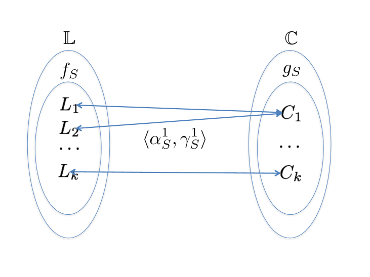
Figure 3: Minimum Cover Mapping Between $f_{S}$ and $g_{S}$

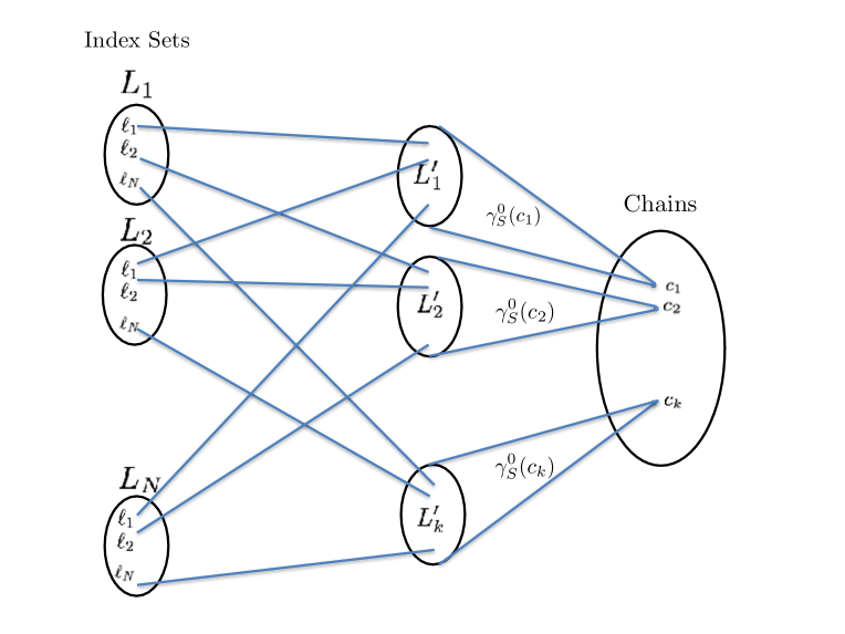
Figure 4: Mapping Between Chains and Index Sets

The two theorems above establish a clear relationship between the two spaces of solutions. We exploit this in our MOSP algorithm.

4.5 An Optimal MOSP Algorithm

To practically apply the theorms in the previous section we introduce a new algorithm that finds a minimal set of indices for an instance $(S,A)$ of MOSP. The algorithm follows from Theorem 3. However, as we only need a single minimum chain cover, our $\gamma_{S}^{1}$ essentially performs a choice/selection of any given minimum chain cover and converts to to a minimum index cover.

We outline the algorithm based on [17] of finding an optimal solution of MCCP in Algorithm 1 for a search set $S$. First, a bi-partite graph is constructed whose vertex sets are the search sets in both partitions of the bi-partite graph (cf. Line 1). Second, an edge between two searches $\mathit{s}$ and $\mathit{s}^{\prime}$ is constructed if $\mathit{s}$ is a strict subset of $\mathit{s}^{\prime}$ . The maximum matching algorithm computes the matching set $E$. Chains are constructed from the matching set by finding the searches that start a chain, i.e., are the smallest element of a chained and do not have a a predecessor. In the algorithm such elements are found in line 4. The smallest element connects via edges immediately and intermediately all searches in the chain. The chain is added to the chain set $C$ in line 6.

Algorithm 2 converts the chains to an index sets. However, due to the relationship summarized in Fig. 4 a single chain may produce several indices. To simply the algorithm and due to only for our problem requiring a single index set we arbitrarily choose a single index from a chain with Choose operation.

1 Function MinChainCover(S):

       Data: Set of Searches $S$

       Result: Minimum Chain Cover $\mathcal{C}$

2       $E:=\textbf{MaxMatching}(S,S,\{(\mathit{s},\mathit{s}^{\prime})\in S\times S\mid\mathit{s}\subset\mathit{s}^{\prime}\})$;

3       initialize ${\mathcal{C}}$ to the empty set;

4       forall $u_{1}\in S:\not\exists(u_{0},u_{1})\in E$ do

5             find max. set $\{(u_{1},u_{2}),(u_{2},u_{3}),\ldots,(u_{k-1},u_{k})\}\subseteq E$ ;

6             add $u_{1}\subset u_{2}\subset u_{3}\ldots\subset u_{k-1}\subset u_{k}$ to ${\mathcal{C}}$ ;

7            

8       end forall

9      return $\mathcal{C}$

10

Algorithm 1 Find Minimum Chain Cover for Searches

1 Function MinIndex(S):

       Data: Set of Searches $S$

       Result: Set of indices to cover searches

2       ${\mathcal{C}}:=\textbf{MinChainCover}(S)$;

3       initialize $L$ to the empty set;

4       forall $\mathit{s}_{1}\subset\mathit{s}_{2}\ldots\subset\mathit{s}_{k-1}\subset\mathit{s}_{k}\in{\mathcal{C}}$ do

5             add $\textbf{Choose}\left(\mathit{s}_{1}\prec\mathit{s}_{2}-\mathit{s}_{1}\prec\ldots\prec\mathit{s}_{k}-\mathit{s}_{k-1}\right)$ to $L$;

6            

7       end forall

8      return $L$

9

Algorithm 2 Compute Minimal Index Set

(a) Matching Problem

(b) Matching Solution

(c) Chain Cover

Figure 5: Motivating Example of Fulkerson’s Maximum Matching Reduction for Dilworth’s Theorem. Partial ordered set is the set of searches $\{x\}$, $\{x,y\}$, $\{x,z\}$, and $\{x,y,z\}$ of relation $A$. Bi-partite construction and solution of maximum matching problem induce a minimal chain cover. The chains induce minimal number of indices $x\prec y\prec z$ and $x\prec z$.

Example 4 (Motivating Example (Cont.))

Consider the motivating example that has the following search set, $S=\{\{x\},\{x,y\},\{x,z\},\{x,y,$ $z\}\}$ that needs to be covered by the smallest set of indices. First, we construct a bi-partite graph with nodes in $S$ in both partitions. The edge set is given by the strict subset relationship between a search pair, i.e., $(\{x\},\{x,y\}),(\{x\},\{x,z\}),(\{x\},$ $\{x,y,z\}),(\{x,y\},\{x,y,z\})$ and $(\{x,z\},\{x,y,z\})$. The bi-partite graph is depicted in Fig. 5(a), and the matching set of the maximal matching solution is depicted in Fig. 5(b). The solution of the maximal matching algorithm is given by the matching set, $E=\{(\{x\},\{x,y\}),(\{x,y\},\{x,y,z\})\}.$ With Algorithm 1 we obtain a chain cover $C$ containing the following chains, $\{x\}\subset\{x,y\}\subset\{x,y,z\}$ and $\{x,z\}$ that is depicted in Fig. 5(c). It is apparent that the two chains are minimal for the cover since the cardinality of the maximum anti-chain (i.e., $\{\{x,y\},\{x,z\}\}$) is also two (cf. Dilworth’s Theorem).

The Algorithm 2 converts the chain cover to indices using a $\gamma$ transformation. The first chain is converted as follows: $\{x\}\subset\{x,y\}\subset\{x,y,z\}$ $\Rightarrow$ $\{x\}\prec\{x,y\}-\{x\}\prec\{x,y,z\}-\{x,y\}$ $\Rightarrow x\prec y\prec z$ Since the smallest element and the set difference are singletons, there exists only a single index that covers the searches of the chain. The second chain consists of a single element $\{x,z\}$. This chain induces two possible indices, i.e., $x\prec z$ and $z\prec x$, and the choice is arbitrary to find an optimal solution for the MOSP problem. An updated index mapping is defined below:

Primitive Predicate	Assigned $\ell$
$x=t_{1}(z)$	$x\prec y\prec z$
$x=t_{1}(y),y=t_{1}(z)$	$x\prec y\prec z$
$x=t_{1}(y),z=t_{1}(z)$	$x\prec z$
$x=t_{1}(z),y=t_{1}(y),z=t_{1}(x)$	$x\prec y\prec z$

5 Datalog Engine Integration

In this section we describe the practicalities of how our technique is integrated into a Datalog engine, using Soufflé as an example. The purpose of this section is to allow our method to be replicated in other high performance Datalog engines [23, 28, 3, 33, 29, 39].

Figure 6: Query optimisation pipeline for input relations $R_{1},\ldots,R_{l}$: index optimiser is invoked for each input relations separately.

The requirements of our approach (1) that queries for a relational database system are expressed in a domain specific language, e.g., SQL [20], Datalog [6], whose underlying query semantics resembles a relational algebra system [12, 1] employing the usual set operators including product, projection, and selection on relations denoted by $R_{1},\ldots,R_{l}$ producing as a result an output relation $R^{\prime}$. (2) an engine converts joins to a nested loop join, that resembles our primitive nested loop joins.

Our approach performs several rewrite transformaitons that we summarize in the pipeline in Fig. 6. In the first step, a query translator converts an input query to a nested loop join (also known as join nested loop join). A nested loop join represents an executable imperative program of the input query constructed by a collection of nested loops. Each loop in the nested loop join enumerates tuples of a relation that occur in the input query, and filters tuples according to loop predicates. The loop body of the most inner loop projects the selected tuples of the loops to a new tuple that will be added to the output relation of the query if the tuple does not exists. The nested loop join is rewritten several times to obtain nested loop joins containing index-operations denoted by range nested loop join.

$\textit{loop}_{1}$: $\textbf{for all}\,t_{1}\in R_{i_{1}}:\varphi_{1}(t_{1})\,\textbf{do}$ $\textit{loop}_{2}$: $\textbf{for all}\,t_{2}\in R_{i_{2}}:\varphi_{2}(t_{1},t_{2})\,\textbf{do}$ $\ldots$ $\textit{loop}_{k}$: for all $t_{k}\in R_{i_{k}}:\varphi_{k}(t_{1},t_{2},\ldots,t_{k})$ do if $\varphi_{k}(t_{1},\ldots,t_{m})\not\in R^{\prime}$ then add $\pi(t_{1},\ldots,t_{m})$ to $R^{\prime}$ endif endfor $\ldots$ endfor endfor

Figure 7: Loop-Nest: a relational algebra query is translated by a query planner to nested loop join; each loop enumerates tuples of a relation and filters selected tuples $t_{1},\ldots,t_{j}$ using a tuple predicate $\varphi_{j}(t_{1},\ldots,t_{j})$. The inner most loop projects selected tuples $t_{1},\ldots,t_{k}$ to a tuple for the output relation $R^{\prime}$. If the tuple does not exist, it will be added to the output relation.

The structure of a nested loop join is shown in Fig. 7. The loops of the nested loop join are labelled by $\textit{loop}_{j}$ for all $j$, $1\leq j\leq k$. The $j$-th loop selects a tuple $t_{j}$ from relation $R_{i_{j}}$ where $i_{j}$ is used to associate the $j$-th loop to one of the input relations $R_{1},\ldots,R_{l}$. The loop predicate $\varphi_{j}(t_{1},\ldots,t_{j})$ is defined over the tuple $t_{j}$ of the current loop and the selected tuples of the outer loops $t_{1}$, …, $t_{j-1}$. The loop predicate filters the tuples of relation $R_{i_{j}}$, i.e., only if the loop predicate holds for the currently selected tuples $t_{1},\ldots,t_{j}$, the loop body is executed with the selected tuples $t_{1},\ldots,t_{j}$. Note that in some cases, the search predicate holds independent of the elements of the tuples (i.e. represents the true value); for this case, all tuples of the relation $R_{i_{j}}$ are enumerated and the search predicate can be omitted.

The query translator selects the best loop order, minimising the iteration space of the nested loop join with the aid of a query planner [1] or user hints. Conditions are hoisted to the outer-most loop where they are still admissible in order to prune the iteration spaces effectively. This technique is also referred to as levelling [5]. After the translation to nested loop joins we have two subsequent transformations that converts the nested loop join to a nested loop join using index operations to speed up the execution of query.

5.1 Search Rewriter

The second step the nested loop join is transformed to a nested loop join with primitive searches, which we refer to as $\sigma$-nested loop join.

In a subsequent transformation step, a primitive search will be replaced by an index operation on relation $R$. Hence, a large number of primitive searches in the nested loop join will make the execution of the query more efficient. The rewriting of the nested loop join to a $\sigma$-nested loop join is mainly a syntactical rewrite step and is shown in Figure 8.

$\textit{loop}_{j}$: $\textbf{for all}\,t_{j}\in R_{i_{j}}:\varphi_{j}(t_{1},\ldots,t_{j})\,\textbf{do}$ $\ldots$ endfor

$\Downarrow$

$\textit{loop}_{j}$: $\textbf{for all}\,t_{j}\in\sigma_{\varphi^{\prime}_{j}}(R_{i_{j}}):\varphi^{\prime\prime}_{1}(t_{1},\ldots,t_{j})\,\textbf{do}$ $\ldots$ endfor

Figure 8: Rewriting of loops in nested loop join using primitive searches: loop predicate $\varphi_{j}$ of the $j$-th loop is replaced by a primitive search with search predicate $\varphi^{\prime}_{j}$ and remaining loop predicate $\varphi^{\prime\prime}_{j}$.

The primitive nested loop join enumerates tuples via the primitive searches, i.e., the original condition $\varphi_{j}$ of the $j$-th loop is broken up into a search predicate $\varphi^{\prime}_{j}$ consisting of a conjunction of equality predicates along with the remaining predicate $\varphi^{\prime\prime}_{j}$, i.e., $\varphi_{j}=\varphi^{\prime}_{j}\wedge\varphi^{\prime\prime}_{j}$. Note that the values of the search predicate $\varphi^{\prime}_{j}$ can only be constants or tuple elements of outer loops (which would be fixed when executing the $j$-th loop); otherwise it cannot be replaced by an index operation. For complex loop predicates there might still be a reduced loop predicate $\varphi^{\prime\prime}_{j}$ that needs to be evaluated for all tuples generated by the primitive search.

Each search predicate is replaced by an index operation to reduce the loop-iteration space further. Note that if no primitive search predicate can be identified in $\varphi_{j}$, the search predicate $\varphi^{\prime}_{j}$ becomes empty and holds for all tuples, i.e., $\sigma_{\textit{true}}(R_{i_{j}})$. Such a pathological case of a primitive search can be rewritten again to the relation $R_{i_{j}}$ itself.

5.2 Index Optimizer

The final step the $\sigma$ nested loop join is converted to range searches. In our approach indices are associated to a single relation only, hence, the index optimisation is performed separately for each input relation. As described in previous sections a lexicographical order is required and the index optimiser chooses the minimal number of lexicographical orders.

Example 5 (Motivating Example (Cont.))

Recall the Datalog rule from the motivating example.

$$B(r,p,q)\leftarrow A(r,p,q),A(q,\_,\_),$$

$$A(p,q,\_),A(p,\_,q),A(q,p,r).$$

The query translator generates the nested loop join for the input query. The order of the loops are chosen such that the iteration space is as small as possible and the conditions are levelled, i.e., hoisted to the outer most loop. For example, the query planner of the query translator could choose following nested loop join for the input query,

$\textit{loop}_{1}$: $\textbf{for all}\,t_{1}\in A\,\textbf{do}$ $\textit{loop}_{2}$: $\textbf{for all}\,t_{2}\in A:t_{2}(x)=t_{1}(z)\,\textbf{do}$ $\textit{loop}_{3}$: $\textbf{for all}\,t_{3}\in A:t_{3}(x)=t_{1}(y)\wedge t_{3}(y)=t_{1}(z)\,\textbf{do}$ $\textit{loop}_{4}$: $\textbf{for all}\,t_{4}\in A:t_{4}(x)=t_{1}(y)\wedge t_{4}(z)=t_{1}(z)\,\textbf{do}$ $\textit{loop}_{5}$: $\textbf{for all}\,t_{5}\in A:t_{5}(x)=t_{1}(y)$ $\wedge t_{5}(y)=t_{1}(y)\wedge t_{5}(z)=t_{1}(x)\,\textbf{do}$ if $t_{1}\not\in B$ then add $t_{1}$ to $B$ endif endfor $\ldots$ endfor

where for each relation instance a loop in the nested loop join is generated. Where there is a variable that binds two attributes together, this is translated to loop predicate $t_{2}(x)=t_{1}(z)$. The outer most loop for this condition is the second outer most loop since it requires information of the tuple element $t_{2}(x)$ which only stabilises in the second outer-most loop. Other conditions of the example are placed accordingly. The projection function $\pi(t_{1},\ldots,t_{5})$ maps the tuples $t_{1},\ldots,t_{5}$ to $t_{1}$, and the if-statement checks whether the tuple $t_{1}$ exists in the output relation $B$. If it does, it adds the tuple to $B$.

The nested loop join is further transformed by the search rewriter to a $\sigma$-nested loop join replacing loop predicates by primitive searches where possible. Since all loop predicates are conjunction of equality predicates, they can all be converted to search predicate of primitive searches. Hence, the output of the search rewriter is given below

$\textit{loop}_{1}$: $\textbf{for all}\,t_{1}\in A\,\textbf{do}$ $\textit{loop}_{2}$: $\textbf{for all}\,t_{2}\in\sigma_{x=t_{1}(y)}(A)\,\textbf{do}$ $\textit{loop}_{3}$: $\textbf{for all}\,t_{3}\in\sigma_{x=t_{1}(y),y=t_{1}(z)}(A)\,\textbf{do}$ $\textit{loop}_{4}$: $\textbf{for all}\,t_{4}\in\sigma_{x=t_{1}(y),z=t_{1}(z)}(A)\,\textbf{do}$ $\textit{loop}_{5}$: $\textbf{for all}\,t_{5}\in\sigma_{x=t_{1}(z),y=t_{1}(y),z=t_{1}(x)}(A)\,\textbf{do}$ if $t_{1}\not\in B$ then add $t_{1}$ to $B$ endif endfor $\ldots$ endfor

for which the remaining loop predicate $C^{\prime\prime}_{1},\ldots,C^{\prime\prime}_{5}$ hold independent of the tuples $t_{1},\ldots,t_{5}$, and are omitted in the $\sigma$-nested loop join above.

In the last step, the primitive searches are rewritten to range searches. The conversion from a $\sigma$-nested loop join to a $\rho$-nested loop join is performed by the index-optimiser. The index optimiser performs the conversion for each input relation separately. Since we only have one input relation (i.e. relation $A$) for our input query, we have only one invocation of the index optimizer.

6 Experiments

In this section we evaluate our technique, which we referred to as Auto-Indexing. We have implemented our approach in the Soufflé Datalog-based analysis tool. We perform two sets of experiments where we compare auto-indexing with a naïve index selection where we select index orders based on syntactical delcarations of relations. We have ommited experiments with no indexing as it results in a time-out in all the experiments and thus confirms the need for the MIA for any reasonably sized program analysis benchmark.

The first set of experiments are conducted on data sets extracted from the DaCapo06 [4] and Julia [41] program benchmarks that represent medium to large programs. For each dataset we perform various points-to analyses taken from the Doop [40] program analysis framework. The Doop analyses are of varying difficulty ranging from the least computational heavy context insensitive analyses (ci, ci+, ci++) and the more computationaly difficult a context-sensitive analyses (o1sh, o2s2h, 3os3h).

The second set of experiments are performed on two very large data sets from industry (OpenJDK 7) and four industrial analyses. Again we compare auto-indexing with a naïve selection. Again, we have ommited experiments with no-indexing. Such large use cases are the primary target of our approach and the catalyst for the development of Soufflé and are typically too large, or at the very least, among the most difficult problems for most Datalog-based tools. We demonstrate that our technique is paramount to Soufflé being able to perform such analyses on giga-scale datasets in a practical amount of time. Moreover, we show that the our reported times perform on a par with the reported results in [15] on the same analysis and dataset. For compressions of Soufflé to other tools we refer the reader to [26, 37].

6.1 Doop Analysis Benchmarks

The results of the improvements of Soufflé our technique (Auto) compared to Soufflé with naïve orderings are summarized in Fig. 10 for run-time improvements and in 10 for memory consumption improvements. These experiments were conducted on a 2.6GHz Intel(R) Core i5-3320M with 8GB physical RAM.

Figure 9: Relative Run-Time Speedup on Doop Benchmarks where timeout is set to 90 minutes.

Figure 10: Relative Memory Usage Improvement on Doop Benchmarks with timed out data points ommited.

The results contain data points for each program in the respective benchmark dataset for a particular points-to analysis (x-axis) and the relative improvement of auto-indexing comapred to naive indexing (y-axis).

The results exlusively demonstrate improvements in both run-time and memory usage. The results indicate that both run-times and memory reductions increase with more difficult datasets, with reasonable index reductions of approx. 15%. For the Dacapo06 dataset we see average memory and run-time improvements of approx. 15% on simpler analyses to approx. 35%, for the more difficult context sensitive analyses with exception to the run-times of 3os3h where larger DaCapo benchmarks result in significant run-time degredations due to the analyses reaching close to the full RAM capacity. The Julia benchmarks largely resulted in timeouts using the nav̈e configuration while auto-index was able to compute a majority of the benchmarks on the availible computing power.

6.2 Large Scale Industrial Case Study : OpenJDK 7

In the following set of experiments we present a very large scale industrial use case. We evaluate Soufflé with our approach on several industrial-scale sized analyses and very large inputs from the OpenJDK 7 codebase. These sets of experiments were conducted on a server node with 18 core Intel(R) Xeon(R) CPU E5-2699 v3 at 2.30GHz and with 378GB of physical RAM.

In Table 2 a set of industrial analysis are outlined along with their number of rules and relations. The first analysis, ci-nocfg, refers to a context insensitive points-to analysis without prior call graph construction. This represents the simplest analysis. The next analysis, ci-pts, which represents a context insensitive points-to analysis with call graph construction. The second last analysis, cs-pts, is a context sensitive points-to that is typically regarded as too difficult for Datalog-based solvers for such large data sets. The last analysis, security, is a security analysis, similar to [11] that is performed to ensure the security of the Java JDK.

In Table 3, we outline the number of code characteristics relevant to our analysis for both industrial code bases. We use two data sets (also known as EDBs) for performing the static program analysis on relational representations of the Java Development Kits (JDK) versions 7 as well as the Java package source code. The large dataset is the OpenJDK 7 b147 library that has 1.4 million program variables, whereas the small data-set has 210 thousand program variables. The algorithmic complexity of the static program analyses used in this paper vary but have at least a cubic worst-case complexity in the number of program variables. For the OpenJDK 7, and the Java package, the output relation sizes can have up to giga-tuples of data with several relations containing hundreds of attributes.

Benchmark	# rul	# rel
ci-nocfg	34	48
ci-pts	160	260
cs-pts	174	292
security	359	600

Table 2: Quantitative Statistics of Analyses

Input	OpenJDK 7	Java
Variables	1,440,875	210,076
Invocations	591,262	81,515
Methods	162,026	29,209
Objects	184,352	21,998
Classes	16,102	6,972

Table 3: OpenJDK7 b147 and Java Package Size

	Run-time (s)			Memory (GByte)			Index Inserts (Mega)
Analysis	Auto	Naïve	Ratio	Auto	Naïve	Ratio	Auto	Naïve	Ratio
ci-ncfg	2.34	3.72	1.59	1.50	1.94	1.29	27.07	52.5	1.94
ci-pts	14.87	17.42	1.17	2.40	3.13	1.30	31.73	51.05	1.61
cs-pts	152.22	444.23	2.92	23.56	49.45	2.10	512.97	971.10	1.89
security	17.31	19.48	1.13	2.77	3.47	1.25	45.01	65.05	1.45

Table 4: Java Package of OpenJDK7 b147

	Run-time (s)			Memory (GByte)			Index Inserts (Mega)
Benchmark	Auto	Naïve	Ratio	Auto	Naïve	Ratio	Auto	Naïve	Ratio
ci-ncfg	64.32	140.30	2.18	31.14	43.55	1.40	1447.65	2882.13	1.99
ci-pts	353.55	656.04	1.86	26.57	42.97	1.62	1020.39	1689.23	1.66
cs-pts	24248.60	n/a	n/a	825.77	n/a	n/a	19578.90	39874.23	2.04
security	52025.00	n/a	n/a	75.30	n/a	n/a	15.33	18.44	1.2

Table 5: OpenJDK 7 b147 dataset

The benchmark results for the small data and large data sets are shown in Table 5 and Table 5, respectively.

For the large benchmark, the programs are executed in parallel using substantial amounts of memory and run-time, i.e., 826GB and 14.5 hours. Note that the naïve approach was not computable for the benchmark “cs-pts” and “security” because of lack of memory and/or running into computation limits. The work of the naïve approach is between 1.2 and 2.04 times more than our new technique that results in speedups between 1.86 and 2.18 depending on the benchmark. For the small dataset all static program analyses are computable. The speedup of our new technique is up to 2.92 and up to 2.1 times less memory is used.

The JDK experiments resulted in a maximum memory reduction of 2.1 times less memory and a maximum speedup of 2.92. As noted before, the OpenJDK 7 data set resulted in a timeout for the context-insensitive and security analysis with the naïve technique while our technique enabled the JDK library to be processed. The memory improvement is due to minimizing redundant index data structures. We attribute the run-time performance to index maintenance costs. Moreover, we highlight that the times achieved using our approach are on a par with the results in [15] using the same data set and analysis. On the java-points-to analysis used for the DaCapo benchmarks our approach managed to provide speed-ups and memory reductions of approx. 20%.

Overall, the experiments show that our technique of automatically generating minimal indices significantly improves both memory usage and run-time in the resultant analyzer. It is no surprise that our technique is more effective on larger, more complex analyses such as the ones in the JDK benchmarks, as such analyses provide more opportunities for index reductions. Such analyses are in fact the main motivation of our technique, in other words, our main motivation is to enable Datalog-based analysis on large industrial sized analysis and data sets, that are typically deemed too difficult for other Datalog-based tools. On the other hand, our approach on the relatively small java-points-to analysis still managed to provide significant speed-ups and memory reductions. While not on the scale of the large scale analysis improvements, we believe this result still has merit and is a notable improvement nevertheless.

7 Related Work

7.1 Datalog Engines

Datalog has been pro-actively researched in several computer science communities [7, 32, 35, 34]. For a comprehensive introduction to Dataog we recommend [1]. Recently, Datalog has regained considerable interest, driven by different applications including data integration, networking, and program analysis. A survey that includes these developments was published recently by [19]. There is likewise a large body of work on Datalog evaluation and Datalog compilation. We refer the reader to the related work of [37] for a general overview of bottom-up engines. Here, we mention some notable state-of-the-art Datalog engines with ordered data structures, namely, LogicBlox [18] and bddbddb [43]. Unlike bddbddb we do not create a global variable order but a per relation order based on a nested loop join, thus solving a polynomial-time problem.

We also believe our MOSP solution can be beneficial to other Datalog engines, even query engines that interpret the Datalog rule can perform the MOSP computation online, since the overhead for the computation is very small we believe this should not greatly affect performance while potentially improving the evaluation significantly. Moreover, we believe that our approach could be in special cases applicable to general query engines that may not have Datalog as a front-end language. For example, our approach could work for bottom-up engines that use SQL defined queries.

Comparisons to LogicBlox: As LogicBlox has traditionally been the default engine of Doop, we can foresee potential interest in comparisons between LogicBlox and Soufflé on Doop benchmarks. In this paper we have omitted such a comparison due to a recent in-depth paper by the authors if Doop [2]. This article gives an extensive overview of the differences between the two engines and provides an indepth comparisson of Soufflé (with auto-index turned on by default) and LogicBlox. The article demonstrates significant improved run-times, for which believe our technqiue plays a significant factor. Our own experiments did not demonstrate any significant deviation from their results in [2]. We only point out that in our experiments Soufflé had lower memory usages compared to LogicBlox.

7.2 Join Algorithms

Join computations are vital for fast Datalog execution. As index selection and join order scheduling are intertwined for query optimization, many state-of-the-art Datalog engines have separated the two for practical reasons. For example, engines such as Socialite [39] and Soufflé [26] allow users to specify the join order. For such engines our technique can be used. Other Datalog engines such as Logicblox [28] use a leapfrog join that, while alleviating users from specifying join order, require users to specify indices manually. Our technique rests on the observation that large Datalog programs usually comprises of significantly less rules than relations. Moreover, of all these rules, usually only a few require manual loop scheduling. These can be identified using a profiler, or alternatively, loop schedules can be automated using heuristic techniques [38]. Therefore, our preference is to fix loop orders rather then indices for a better user experience. The preference for this design choice has been confirmed from the Soufflé user community.

7.3 Index Selection

In the context of traditional relational databases, the general problem of automatically selecting indices for a set of queries, referred to in the literature as the index selection problem (ISP) [36, 13, 24, 27], is well studied and has been shown to be NP-hard [30]. State-of-the-art techniques typically formulate ISP as a variation of the $0$-$1$ knapsack problem. Knapsack formulations of ISP assume a relational database setup, i.e., relations are stored in secondary storage and queries are executed on normalized data. Indices are “packed” by balancing the overall execution time of queries for an index configuration (i.e., a subset of indices that influence the performance of a query), and the costs of index maintenance. All possible index configurations are reflected in form of $0-1$ decision variables. Constraints in the index selection problem ensure that at most one index configuration is chosen for a query, and other constraint forces an index to be packed if the index occurs in a selected index configuration of a query. The objective function of ISP is the profit of selected index configuration of queries minus the cost of maintaining selected indices. Note that if the relations are normalized, the set of indexes will be small in relational databases, and hence ISP as a combinatorial optimisation problem becomes viable.

The standard ILP model for ISP may be expressed as the following ILP model below:

$$\max =\sum_{q\in Q}\sum_{k\in K}g_{qk}x_{qk}-\sum_{i\in I}f_{i}y_{i}$$

s.t. $$\sum_{k\in K}x_{qk}\leq 1, \forall k\in K$$

$$x_{qk}\leq y_{i}, \forall q\in Q,k\in K,i\in I:i\in k$$

$$x_{qk},y_{i}\in\{0,1\}, \forall q\in Q,k\in K,i\in I$$

Here $I$ be the set of indices, $Q$ the set of all queries, and $K$ are the index configurations. An index configuration $k$ is a subset of the index set $I$. The $0$-$1$ decision variable $x_{qk}$ determines whether configuration $k$ for query $q$ is selected, and the $0$-$1$ variable $y_{i}$ determines whether index $i$ is selected. The first constraints of the ILP model ensures that at most one index configuration is chosen for a query $q$, and the second constraint forces variable $y_{i}$ to be set to one if there exists a decision variable $x_{qk}$ whose configuration $k$ contains index $i$. The objective function is the profit of the configurations over all queries minus the cost of maintaining indices where $g_{qk}$ is the profit of index configuration $k$ for query $q$, and $f_{i}$ are the maintenance costs for index $i$.

Automated index selection was studied in the context of self-tuning database systems [9]. As choosing an optimal index configuration is NP-complete in the general case [30], the mechanisms that were introduced starting in the late 90s used the existing cost model and some heuristics to select/propose indices for a workload. Index advisors were implemented in all major relational database systems [10, 42, 14]. Other models uses the Knapsack problem as a vehicle for finding an optimal solution [24] and more exotic approaches use genetic algorithms [27] to find sub-optimal indices. The work of [22] proposes an extension of prior index optimisation models where there are multiple-candidates available for attributes, and Gündem shows that the optimisation model is NP-hard, and provide an approximation algorithm which is bounded by a logarithmic time order. Older works [36, 13] provide some probabilistic modelling for selecting secondary indices and some ad-hoc approaches. A related problem is the index selection for views for example in OLAP domains [21]. Our index selection problem differs from the classic ISP literate and to the best of our knowledge is the first formulation of such as problem. In our case, we are restricted to support primitive searches only. Primitive searches occur in equi-joins and simple value queries. We further have a maximal index assumption, i.e., each primitive search is covered by at least one index. This assumptions is important for high-performance systems which needs to accelerate all searches and the question is to minimise the indices to cover all searches. Since our problem differs to existing approaches, we obtain an optimal algorithm that exhibits a polynomial worst-case execution time. The effect of our optimisation reduces the cost of maintaining indices. It relies on a pre-determined clause body order and assumes all relations are indexed in memory. With modern memory systems this assumption becomes very much feasible and leads to large performance improvements. Secondly, the nature of Datalog restricts search predicate of primitive searches, i.e., the search predicate has to be an equality predicate over the attributes of the relation. The traditional formulations of the model do not capture this restrictions as they are too coarse-grained in a mathematical sense. While not related to index selection the approach in [25] uses Dilworths theorem as a fast reachibility algorithm to process graph reachability queries.

8 Conclusion

We have presented an join computation technique that computes the minimal set of indices a given relation. The proposed algorithm runs in polynomial time due to exploiting a relationship to Dilworth’s problem: Instead of finding indices directly, and searching in a double-exponential space for finding them, we construct a partial order over the primitive searches. A minimum chain cover in the partial order over the primitive searches construct the minimal set of indices, indirectly. We have demonstrated the feasibility of our approach through experiments using Soufflé, a Datalog-based static analysis tool. In future, we plan to explore the possibility of adapting our technique to general in-memory relational database engines, as well.

9 Acknowledgments

We would like to thank Oracle Labs, Alan Fekete, Byron Cook, Chenyi Zhang and all our anonymous reviewers.

Appendix A Proofs

A.1 Proofs from Section 3

Proof A.4 (Lemma 1).

Let us assume a index of size $k$ i.e., $\ell=x_{1}\prec\dots\prec x_{k}$ and a relation $R$ of a fixed size. By induction on size of $\ell$ we have: Base case (size $1$) : it is trivial that

$$\{t\in R\ |\ t(x_{1})=v_{1}\}=\{t\in R\ |\ lb(v_{1})\sqsubseteq_{x_{1}}t\sqsubseteq_{x_{1}}ub(v_{1})\}.$$

Now we construct the IH (size is $n$) we hence

$$\{\ t\in R\ |\ t(x_{1})=v_{1}\wedge\dots\wedge t(x_{n})=v_{n}\}=$$

$$\{\ t\in R\ |\ lb(v_{1},\dots,v_{n})\sqsubseteq_{\ell}t\sqsubseteq_{\ell}ub(v_{1},\dots,v_{n})\}\text{ where }$$

$$\ell=x_{1}\prec\dots\prec x_{n}$$

Assuming the IH, and letting $k=n+1$ we have

$$\{\ t\in R\ |\ t(x_{1})=v_{1}\wedge\dots\wedge t(x_{n})=v_{n}\wedge t(x_{n+1})\}=$$

$$\{\ t\in R\ |\ lb(v_{1},\dots,v_{n},v_{n+1})\sqsubseteq_{\ell}t\sqsubseteq_{\ell}ub(v_{1},\dots,v_{n},v_{n+1})\}.$$

We can rewrite this as:

$$\{\ t\in\sigma_{x_{n+1}}(R)\ |\ t(x_{1})=v_{1}\wedge\dots\wedge t(x_{n})=v_{n}\}=$$

$$\{\ t\in\sigma_{\rho(x_{n+1},lb(v_{n+1}),ub(v_{n+1}))}(R)\ |$$

$$\ lb(v_{1},\dots,v_{n})\sqsubseteq_{x_{n+1}}t\sqsubseteq_{x_{n+1}}ub(v_{1},\dots,v_{n})\}.$$

Hence by IH and the base case it holds.

If $\ell$ is $x_{1}\prec\dots\prec x_{k}\prec x_{s}$ the property still holds as the bounds for the $x_{s}$ are set to the infima ($\bot$) and suprema ($\top$) for $a$ and $b$, respectively. Hence retaining the property.

A.2 Proofs from Section 4

A.2.1 Lemma Proofs

Proof A.5 (of Lemma 2).

We can bound the cardinality of the set of all possible sequences as follows,

$$m!=|\textsf{Pm}(A)| \leq\left|\bigcup_{X\subseteq A,X\not=\emptyset}\textsf{Pm}(X)\right|$$

$$=\sum_{X\subseteq A,X\not=\emptyset}|X|!$$

$$=\sum_{1\leq i\leq m}\binom{m}{i}i!$$

$$=m!\sum_{1\leq i\leq m}\frac{1}{(m-i)!}$$

$$=m!\sum_{0\leq i\leq m-1}\frac{1}{i!}$$

$$\leq m!\sum_{i\geq 0}\frac{1}{i!}$$

$$=\mathsf{e}\cdot m!$$

The lower bound is given by the $m!=|\textsf{Pm}(X)|$ since $\textsf{Pm}(X)\subseteq L$. For the upper bound, we sum up the cardinalities of permutations over all subsets except the empty set. We reorder the sum by summing up the permutations of subsets that have cardinality $i$, i.e., there are $\binom{m}{i}$ subsets of cardinality $i$. By simplifying the binom and factoring out $m!$ we can rearrange the summation such that the index runs from $0$ to $m-1$. Since the numbers of the series $\frac{1}{i!}$ are positive and converge, we can extend the range to infinity to obtain an upper bound and the sum converges to the Euler number. Hence, $\mathsf{e}\cdot m!$ is an upper bound on the number of sequences for $m$ attributes.

Proof A.6 (of Lemma 3).

By construction

Proof A.7 (of Lemma 4).

By contradiction. (Case 1). Assume $|\alpha_{S}^{1}(L)|>|L|.$ This is not possible because function $\alpha_{S}^{0}$ maps one index to exactly one chain. Hence, due to the pigeonhole principle there can be at most $|L|$ different chains in $\alpha_{S}^{1}(L)$. (Case 2). Assume $|\alpha_{S}^{1}(L)|<|L|.$ Hence there must exist $l_{1}\not=l_{2}\in L$, such that $\alpha_{S}^{0}(l_{1})=\alpha_{S}^{0}(l_{2})$, and $\alpha_{S}^{1}(L\setminus\{l_{2}\})=\alpha_{S}^{1}(L)$. However, due to Lemma 6, $\textbf{c-cover}(\alpha_{S}^{1}(L))\Rightarrow\textbf{c-cover}_{S}(\alpha_{S}^{1}(L\setminus\{l_{2}\})\Rightarrow\textbf{l-cover}_{S}(L\setminus\{l_{2}\})$. Hence, $L\not\in f(S)$ because $|L|$ is not minimal, i.e., $L\setminus\{l_{2}\}$ represents a smaller solution for which $\textbf{l-cover}(L\setminus\{l_{2}\})$ holds. As a consequence of (Case 1) and (Case 2), the lemma holds.

Proof A.8 (of Lemma 5).

By definition.

$$\textbf{l-cover}_{S}(L) \Leftrightarrow \forall s\in S:\exists l\in L:\textbf{prefix}_{|s|}(l)=s$$

$$\Leftrightarrow \forall s\in S:\exists l\in L:s\in\alpha_{S}^{0}(l)$$

$$\Leftrightarrow \forall s\in S:\exists c\in\alpha_{S}^{1}(L):s\in c$$

$$\Leftrightarrow \textbf{c-cover}(\alpha_{S}^{1}(L))$$

Proof A.9 (of Lemma 6).

By definition.

$$\textbf{c-cover}_{S}(C)\Rightarrow\forall\mathit{s}\in S:\exists c\in C:\mathit{s}\in c$$

$$\Rightarrow \forall L\in\gamma_{S}^{1}(C):\forall\mathit{s}\in S:\exists c\in C:\mathit{s}\in c$$

$$\Rightarrow \forall L\in\{\{\ell_{1},\dots,\ell_{k}\}\ \mid\ \ell_{1}\in\gamma_{S}^{0}(c_{1}),\dots,\ell_{k}\in\gamma_{S}^{0}(c_{k})\}:$$

$$\forall s\in Q:\exists c\in C:s\in c$$

$$\Rightarrow \forall L\in\{\{\ell_{1},\dots,\ell_{k}\}\ \mid\ c_{1}\subseteq\alpha_{S}^{0}(\ell_{1}),\dots,c_{k}\subseteq\alpha_{S}^{0}(\ell_{k})\}:$$

$$\forall s\in S:\exists c\in C:s\in c$$

$$\Rightarrow \forall L\in\gamma_{S}^{1}(C):\forall s\in S:\exists l\in L:s\in\alpha_{S}^{0}(\ell)$$

$$\Rightarrow \forall L\in\gamma_{S}^{1}(C):\textbf{l-cover}_{S}(L)$$

A.2.2 Theorem Proofs

Proof A.10 (of Theorem 2).

If $L\in f_{S}$ then $L$ is a l-cover and is minimal. By Lemma 4 and Lemma 5, cardinality and cover is preserved. Hence we have a chain $C\equiv\alpha_{S}^{1}(L)$ that is a c-cover and minimal due to the fact that if it was not minimal, there would be an $|L^{\prime}|<|L|$ by Lemma 4. However, this would violate our assumption that L is in $f_{S}$.

Proof A.11 (of Theorem 3).

We instantiate $C_{i}$ and $L_{i}$ from the domains of $g_{S}$ and $\gamma_{S}^{1}(C_{i})$, respectively. Given that c-cover_S($C_{i}$) holds and that $\forall C\in g_{S}/C_{i}:|C|=|C_{i}|$, we want to show l-cover($L_{i}$) holds and that $\forall L\in\gamma_{S}^{1}(C_{i})/L_{i}:|L|=|L_{i}|$. The proof of l-cover_S($L_{i}$) follows by Lemma 6. Showing minimality follows from Lemma 3 and the observation that $\gamma_{S}^{1}(C)$, where $|C|=k$, creates k-size upper-bound index sets. Therefore, $|L_{i}|\leq|C|=k$. We also know by Lemma 4 that $C^{\prime}\equiv|\alpha_{S}^{1}(L_{i})|$ and $|C^{\prime}|=|L_{i}|$. But $C^{\prime}$ can’t be smaller than $C$ as $C$ is in $g_{S}$ (min chains) hence $|C|=|L_{i}|$ and $L_{i}$ must be minimal and an l-cover. We therefore conclude it is in $f_{S}$

References

- [1] S. Abiteboul, R. Hull, and V. Vianu. Foundations of Databases. Addison-Wesley, 1995.
- [2] T. Antoniadis, K. Triantafyllou, and Y. Smaragdakis. Porting doop to soufflé: A tale of inter-engine portability for datalog-based analyses. In Proceedings of the 6th ACM SIGPLAN International Workshop on State Of the Art in Program Analysis, SOAP 2017, pages 25–30, New York, NY, USA, 2017. ACM.
- [3] K. Bierhoff. Alias analysis with bddbddb, star project report, 17-754 analysis of software artifacts. www.cs.cmu.edu/~aldrich/courses/654/tools/bierhoff-bddbddb-05.pdf, 2005.
- [4] S. M. Blackburn, R. Garner, C. Hoffman, A. M. Khan, K. S. McKinley, R. Bentzur, A. Diwan, D. Feinberg, D. Frampton, S. Z. Guyer, M. Hirzel, A. Hosking, M. Jump, H. Lee, J. E. B. Moss, A. Phansalkar, D. Stefanović, T. VanDrunen, D. von Dincklage, and B. Wiedermann. The DaCapo benchmarks: Java benchmarking development and analysis. In OOPSLA ’06: Proceedings of the 21st annual ACM SIGPLAN conference on Object-Oriented Programing, Systems, Languages, and Applications, pages 169–190, New York, NY, USA, Oct. 2006. ACM Press.
- [5] B.Scholz, K.Vorobyov, P.Krishnan, and T.Westmann. A datalog source-to-source translator for static program analysis: An experience report. Australasian Software Engineering Conference, 2015.
- [6] S. Ceri, G. Gottlob, and L. Tanca. What you always wanted to know about datalog (and never dared to ask). IEEE Trans. on Knowl. and Data Eng., 1(1):146–166, Mar. 1989.
- [7] S. Ceri, G. Gottlob, and L. Tanca. What you always wanted to know about datalog (and never dared to ask). IEEE Transactions on Knowledge and Data Engineering, 1(1):146–166, 1989.
- [8] S. Chaudhuri and V. Narasayya. An efficient, cost-driven index selection tool for microsoft sql server. Very Large Data Bases Endowment Inc., August 1997.
- [9] S. Chaudhuri and V. Narasayya. Self-tuning database systems: A decade of progress. In Proceedings of the 33rd International Conference on Very Large Data Bases, VLDB ’07, pages 3–14. VLDB Endowment, 2007.
- [10] S. Chaudhuri and V. R. Narasayya. An efficient cost-driven index selection tool for microsoft sql server. pages 146–155, Athens, Greece, 1997. Morgan Kaufmann.
- [11] C. Cifuentes, A. Gross, and N. Keynes. Understanding caller-sensitive method vulnerabilities: a class of access control vulnerabilities in the java platform. In A. Møller and M. Naik, editors, Proceedings of the 4th ACM SIGPLAN International Workshop on State Of the Art in Program Analysis, SOAP@PLDI 2015, Portland, OR, USA, June 15 - 17, 2015, pages 7–12. ACM, 2015.
- [12] E. F. Codd. A relational model of data for large shared data banks. Commun. ACM, 13(6):377–387, June 1970.
- [13] D. Comer. The difficulty of optimum index selection. ACM Trans. Database Syst., 3(4):440–445, Dec. 1978.
- [14] B. Dageville, D. Das, K. Dias, K. Yagoub, M. Zaït, and M. Ziauddin. Automatic SQL tuning in oracle 10g. pages 1098–1109, Toronto, Canada, September 2004. Morgan Kaufmann.
- [15] J. Dietrich, N. Hollingum, and B. Scholz. Giga-scale exhaustive points-to analysis for java in under a minute. In J. Aldrich and P. Eugster, editors, Proceedings of the 2015 ACM SIGPLAN International Conference on Object-Oriented Programming, Systems, Languages, and Applications, OOPSLA 2015, part of SPLASH 2015, Pittsburgh, PA, USA, October 25-30, 2015, pages 535–551. ACM, 2015.
- [16] R. Dilworth. A decomposition theorem for partially ordered sets. Ann. Math. (2), 51:161–166, 1950.
- [17] D. R. Fulkerson. Note on dilworth’s decomposition theorem for partially ordered sets. Proceedings of the American Mathematical Society, 7(4):pp. 701–702, 1956.
- [18] T. J. Green, M. Aref, and G. Karvounarakis. LogicBlox, platform and language: A tutorial. In Datalog in Academia and Industry - Second International Workshop, volume 7494 of Lecture Notes in Computer Science, pages 1–8. Springer, September 2012.
- [19] T. J. Green, S. S. Huang, B. T. Loo, and W. Zhou. Datalog and recursive query processing. Foundations and Trends in Databases, 5(2):105–195, 2013.
- [20] J. Groff and P. Weinberg. SQL The Complete Reference, 3rd Edition. McGraw-Hill, Inc., New York, NY, USA, 3 edition, 2010.
- [21] H. Gupta, V. Harinarayan, A. Rajaraman, and J. D. Ullman. Index selection for olap. pages 208–219, 1997.
- [22] T. Gündem. Near optimal multiple choice index selection for relational databases. Computers and Mathematics with Applications, 37(2):111 – 120, 1999.
- [23] K. Hoder, N. Bjørner, and L. De Moura. Z: An efficient engine for fixed points with constraints. In Proceedings of the 23rd international conference on Computer aided verification, CAV’11, pages 457–462, Berlin, Heidelberg, 2011. Springer-Verlag.
- [24] M. Ip, L. Saxton, and V. Raghavan. On the selection of an optimal set of indexes. Software Engineering, IEEE Transactions on, SE-9(2):135–143, March 1983.
- [25] H. V. Jagadish. A compression technique to materialize transitive closure. ACM Trans. Database Syst., 15(4):558–598, Dec. 1990.
- [26] H. Jordan, B. Scholz, and P. Subotic. Soufflé: On synthesis of program analyzers. In S. Chaudhuri and A. Farzan, editors, Computer Aided Verification - 28th International Conference, CAV 2016, Toronto, ON, Canada, July 17-23, 2016, Proceedings, Part II, volume 9780 of Lecture Notes in Computer Science, pages 422–430. Springer, 2016.
- [27] J. Kratica, I. Ljubic, and D. Tošic. A genetic algorithm for the index selection problem. In Proceedings of the 2003 International Conference on Applications of Evolutionary Computing, EvoWorkshops’03, pages 280–290, Berlin, Heidelberg, 2003. Springer-Verlag.
- [28] I. LogicBlox. Declartive cloud platform for applications that combine transactions & analytics. http://www.logicblox.com.
- [29] G. Phipps, M. A. Derr, and K. A. Ross. Glue-nail: A deductive database system. In Proceedings of the 1991 ACM SIGMOD International Conference on Management of Data, SIGMOD ’91, pages 308–317, New York, NY, USA, 1991. ACM.
- [30] G. Piatetsky-Shapiro. The Optimal Selection of Secondary Indices is NP-complete. SIGMOD Rec., 13(2):72–75, Jan. 1983.
- [31] W. Pijls and R. Potharst. Another note on dilworth’s decomposition theorem. Journal of Discrete Mathematics, 2013:4, 2013.
- [32] R. Ramakrishnan, D. Srivastava, and S. Sudarshan. Efficient bottom-up evaluation of logic programs. In P. Dewilde and J. Vandewalle, editors, Computer Systems and Software Engineering, pages 287–324. Springer US, 1992.
- [33] R. Ramakrishnan, D. Srivastava, S. Sudarshan, and P. Seshadri. Implementation of the coral deductive database system. SIGMOD Rec., 22(2):167–176, June 1993.
- [34] R. Ramakrishnan and J. D. Ullman. A survey of deductive database systems. Journal of Logic Programming, 23(2):125–149, 1995.
- [35] K. Ramamohanarao and J. Harland. An introduction to deductive database languages and systems. Journal of Very Large Data Bases, 3(2):107–122, 1994.
- [36] M. Schkolnick. The optimal selection of secondary indices for files. Information Systems, 1(4):141 – 146, 1975.
- [37] B. Scholz, H. Jordan, P. Subotic, and T. Westmann. On fast large-scale program analysis in datalog. In A. Zaks and M. V. Hermenegildo, editors, Proceedings of the 25th International Conference on Compiler Construction, CC 2016, Barcelona, Spain, March 12-18, 2016, pages 196–206. ACM, 2016.
- [38] P. G. Selinger, M. M. Astrahan, D. D. Chamberlin, R. A. Lorie, and T. G. Price. Access path selection in a relational database management system. In Proceedings of the 1979 ACM SIGMOD International Conference on Management of Data, SIGMOD ’79, pages 23–34, New York, NY, USA, 1979. ACM.
- [39] J. Seo, J. Park, J. Shin, and M. S. Lam. Distributed socialite: A datalog-based language for large-scale graph analysis. Proc. VLDB Endow., 6(14):1906–1917, Sept. 2013.
- [40] Y. Smaragdaiks, M. Bravenboer, and G. Kastrinis. Doop: A framework for java pointer analysis. http://doop.program-analysis.org/.
- [41] F. Spoto. The Julia Static Analyzer for Java, pages 39–57. Springer Berlin Heidelberg, Berlin, Heidelberg, 2016.
- [42] G. Valentin, M. Zuliani, D. C. Zilio, G. M. Lohman, and A. Skelley. DB2 advisor: An optimizer smart enough to recommend its own indexes. In ICDE, pages 101–110, 2000.
- [43] J. Whaley, D. Avots, M. Carbin, and M. S. Lam. Using datalog with binary decision diagrams for program analysis. In Proceedings of the Third Asian conference on Programming Languages and Systems, APLAS’05, pages 97–118, Berlin, Heidelberg, 2005. Springer-Verlag.