About Superrotation in Venus

Abstract

In this work we study in a general view slow rotating planets as Venus or Titan which present superrotating winds in their atmospheres. We are interested in understanding what mechanisms are candidates to be sources of net angular momentum to generate this kind of dynamics.

In particular, in the case of Venus, in its atmosphere around an altitude of 100 Km relative to the surface, there exists winds that perform a full rotation around the planet in four terrestrial days, whereas the venusian day is equivalent to 243 terrestrial ones. This phenomenon called superrotation is known since many decades. However, its origin and behaviour is not completely understood. In this article we analise and ponderate the importance of different effects to generate this dynamics.

year number number identifier Date text]date

LABEL:FirstPage101 LABEL:LastPage#1102

I Introduction

Superrotation in Venus is an effect known since forty or more years. However, the origin and mechanism of sustenance of these fast winds is still an open question. In this report we want to review different proposals for the causes of this phenomenon, and to introduce a simple model to clarify the basic physical effects necessary to sustain the winds by sun irradiation.

The upper atmosphere of a planet is regarded as the region of the atmosphere whose structure and dynamics (temperature and density distribution, composition and winds) are governed by the direct absorption of solar radiation. The diversity and complexity of the processes taking place in the upper atmospheres have made it necessary to develop their study into a-separate branch of geophysics and astrophysics—aeronomy, which uses many branches of physics and some branches of chemistry. The study of upper atmospheres has both practical and theoretical interest. The knowledge of the characteristics of the charged components of the upper atmosphere (which constitutes the ionosphere of the planet) is needed to improve radio communications and radio navigation (including space navigation); the knowledge of the characteristics of the neutral upper atmosphere is needed to determine the trajectories and lifetimes of artificial satellites and the trajectories of space probes that enter the atmosphere. Clarification of the mechanisms by which the influence of solar activity is transmitted through the upper atmosphere to the troposphere is one of the important tasks in the problem of solar-terrestrial relations. Comparative study of the upper atmospheres of different planets and, in particular, of the dissipation of gases from the atmospheres assists in clarifying the problem of the evolution of planetary atmospheres. The dynamics of the Venus atmosphere presents a major unsolved problem in planetary science: the so-called superrotation of the lower atmosphere and its transition to solar-antisolar circulation in the upper atmosphere. In general the dividing line between the lower and upper atmosphere at 90–100 km altitude (pressure 0.39 to 0.028 mbar), the base of the day-side thermosphere.) Superrotation has also been observed in the atmosphere of Titan, the only other slowly rotating world with a substantial atmosphere known at present. In this case also the transition to a different circulation in the upper atmosphere is also apparent but not well understood. Thus, the issues discussed below may be generic to any slowly rotating terrestrial planet’s atmosphere.

I.1 Comparison with Earth

Venus is one of the terrestrial planets, together with Earth and Mars, and has similar mass and radius to those of Earth. Probably at the beginning of its history it had a similar atmosphere to our planet. For unknown reasons Venus has a slow retrograde rotation respect Earth.

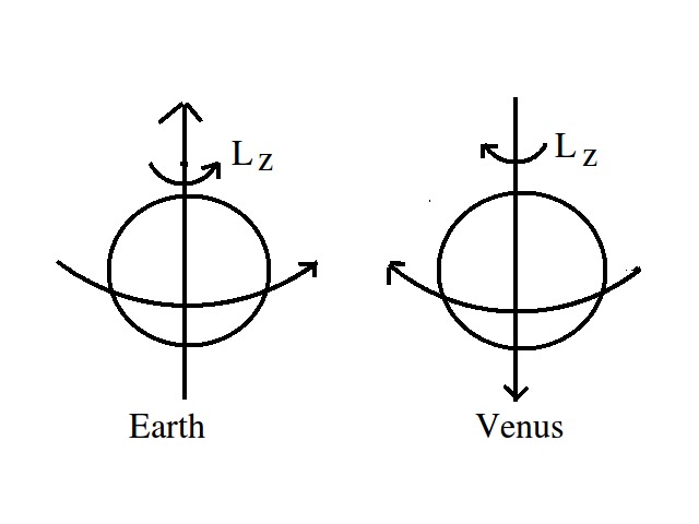
Figure 1: Sketch of retrograde movement of Venus.

Apparently the magnetic dynamo in Venus is turned off, and thus its atmosphere is completely exposed to the action of the solar wind, which lead to several authors to speculate an initial loss of hydrogen and oxygen, that in principle explains the absence of water. However, enough concentrations of nitrogen and carbon exist to generates a greenhouse effect, maintaining a dense and acid atmosphere compared with that of our planet. Temperature varies along altitude, and due to superrotation there are not strong fluctuations between day and night sides in the upper atmospheric levels. One point to note is that the difference in Albedo between day and night is extreme. The radiation in those regions is approximately that of a black body and a white body, respectively.

Table 1: Typical values of Earth and Venus (Peralta et al., 2014).

Scale	Symbol	Venus	Earth
Radius (m)	$r$	$6,051\cdot 10^{6}$	$6\cdot 10^{6}$
Magnetic Field (G)	B	$\sim 10^{-5}$	0,5
Rotation period (earth days)	T	243	1
Equatioral surface velocity (m/s)	$v_{eq}$	1.8	465
Super Wind Periodicity (earth days)	$T_{sw}$	4	-
Temperature Range (K)	T	{228 - 773}	{184 -331}
CO2 (%)		96	0,04
N2 (%)		3	78,1
Pressure at Troposphere level (Earth Atmosphere)	P	92	1
Mass (Kg)	M	$4,9\cdot 10^{24}$	$5,98\cdot 10^{24}$
Density ($g/cm^{3}$)	$\rho$	5,24	5,51
Days/Year (local)		1,92	365,25
eccentricity		0	0,016
Albedo		0,65	38
Distance to the Sun (AU)		0,723	1

Table 2: Sketch of retrograde movement of Venus.

II Early attempts

In this section we describe some essential and basic characteristics of Venusian atmosphere and its interaction with the surrounding ambient. The atmosphere presents two dynamic regimes, zonal superrotation in the troposphere and mesosphere (Gierasch et al., 1997) and solar-antisolar circulation trough the terminator line in thermosphere (Bougher et al., 1997), (Peralta Calvillo, 2008).

II.1 Solar Wind Interaction

Although Venus has apparently no magnetic field of its own, the solar wind in the higher atmosphere levels generates an induced magnetosphere. The schematic cartoon is shown in Figure 2.

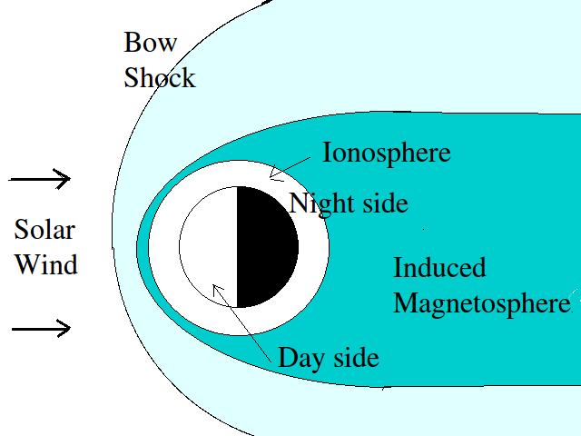
Figure 2: Scheme of the induced magnetosphere structure of Venus due to the action of solar wind.

II.2 Atmospheric dynamics

We call “neutral atmosphere” that corresponding to intermediate altitudes where the hydrodynamic approximation is valid, i.e. we can use the Navier-Stokes equations. Coriolis force due to the slow rotation of Venus is negligible. It means that the cyclostrophic approximation where pressure gradient is comparable to centrifugal force, $\nabla p\sim f_{centrifuge}$, is valid, in opposition to the Earth where the geostrophic approximation, in which the pressure gradient is proportional to Coriolis force $\nabla p\sim f_{coriolis}$, is more appropriate.

The atmosphere is stratified with a layer of clouds around 100 Km of altitude that has essentially different absorptions rates and stronger winds.

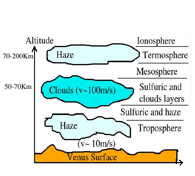
Figure 3: Cartoon of venusian atmospherical levels. The presence of superrotating winds are at the cloud layer.

In the clouds layer, speed winds are maximal, of the order of 120m/s, as well as the absorption of solar irradiance. At lower layers the speed of the winds decrease abruptly and are close to co-rotation with the planetary surface, sixty times below that in the cloud layer. Above the clouds the wind velocity also decreases.

Using the instrument SOIR on board the ESA Venus Express, Mahieux et al, (2012) (Mahieux et al., 2012) measured different carbon dioxide densities (the main component of the atmosphere) in the Venus terminator different profiles. They established temperature profiles in this region for different latitude and altitudes, some of the results are shown in Figure 4.

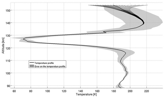
Figure 4: Temperature vs altitude profile at Venus terminator. Continuous line is the temperature and grey region is the error. (Mahieux et al., 2012)

II.3 Atmospheric Cells

These cells transports heat from the equator to the poles by convection, the scheme is shown in Figure 5. The warm gas travels to the poles and closes the cell transporting cold gas which toward the equator al low altitudes. Essentially, there are four cells, two in the northern hemisphere and two in the southern one. The two cells in each hemisphere have a separatrix in the solar (midday) and anti-solar lines (midnight). Over these cells, in the thermosphere, the circulation cells from solar to anti-solar points takes place, the so called transterminator flow. Close to the poles in the mesosphere polar vortices and polar collars are present.

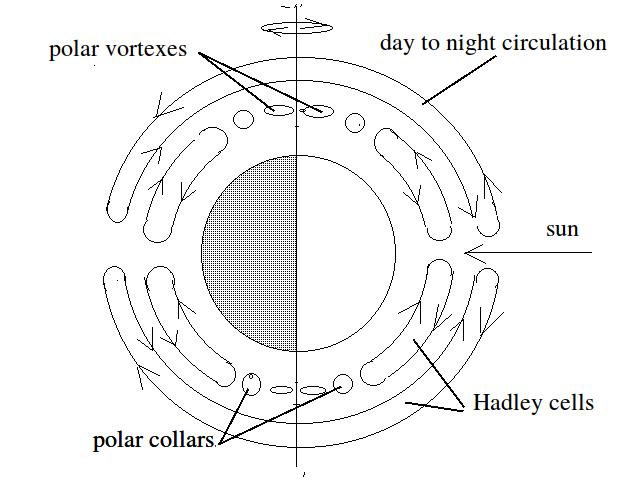
Figure 5: Scheme of Hadley convective cells and superrotating winds.

III Superrotation

To have superrotation, it is necessary to build up net angular momentum over the whole atmosphere around the planet. Also, a stationary balance between sources of angular momentum and diffusive effects to maintain an equilibrium in time is necessary too. In this section we are going to mention some of these effects to evaluate their role in this dynamics.

III.1 Solar wind influence

On Mars and Venus the solar wind (the flux of solar plasma) has a very important influence on the atmosphere because of the weak magnetic fields of these planets. According to the measurements, the magnetic fields of Mars and Venus are about $10^{-4}$ of the terrestrial magnetic field; Mars apparently has an intrinsic magnetic moment while the magnetic field of Venus is induced by the effect of the solar wind on the ionosphere. (Dolginov et al., 1968), (Dolginov et al., 1969), (Dolginov and et al., 1972), (Bridge et al., 1967), (Dolginov et al., 1973a) and (Dolginov et al., 1973b).

The nature of the influence of the solar wind has not yet been completely clarified, though the main features are as follows (Spreiter and Alksne, 1970), (Spreiter et al., 1970), (Cloutier and Daniell, 1973), (Cloutier et al., 1974) and (Bauer and Hartle, 1973). The plasma of the solar wind (with concentrations of a few particles per 1 cm³, frozen magnetic field $\overline{B}_{sw}5-20nT$, and velocities of about 300-600 km/sec near Venus and Mars) compresses the ionospheric plasma on the dayside, forming a sharp boundary— the plasmopause or ionopause—while on the nightside it forms the tail of the plasmosphere. The streamlines of the solar wind are deflected, so that it flows round the plasmosphere. Above and along the flux a shock wave is formed, in which the velocity, magnetic field, and temperature of the solar wind change abruptly. The plasmopause on Venus was discovered at an altitude of about 500 km by means of the radar-occultation experiments with Mariner 5. The presence of a shock wave near Mars and Venus has been confirmed by magnetic and plasma measurements by Venera 4 and 6, Mariner 4 and 5, and Mars 2 and 3 (Smith et al., 1965), (Smith, 1969), (Gringauz et al., 1968), (Gringauz et al., 1970), (Gringauz et al., 1973), (Gringauz and et al., 1972), (Gringauz and et al., 1973) and (Vaisberg and Bogdanov, 1974). The shape of the shock wave agrees satisfactorily with the one calculated in the framework of the hypersonic gas-dynamic model.

The position of the plasmopause is determined in the hydrodynamic approximation by the condition of balance of the dynamic pressure of the solar wind and the pressure of the ionosphere:

$$\varkappa n_{sw}m_{sw}v_{sw}\cos^{2}\left(\zeta\right)+\frac{\overline{B}_{sw}^{2}}{8\pi}=k\left(n_{e}T_{e}+n_{i}T_{i}\right)+\frac{\overline{B}^{2}}{8\pi}$$ (1)

where $n_{sw}$, $m_{sw}$, $v_{sw}$, $B_{sw}$ are the concentration, the mean mass of the particles, the velocity, and the magnetic field in the solar wind, $\varkappa\sim$0.88 for the flow considered here; $n_{e}$, $n_{i}$, $T_{e}$, $T_{i}$ are the concentrations and temperatures of the ionospheric electrons and ions, and $\overline{B}$ is the magnetic field in the ionosphere; $\zeta$ is the angle between the outer normal to the mesopause and the velocity of the unperturbed solar wind.

Note that neglecting the interaction between the solar wind and the neutral particles simplifies the real picture since although the cross sections of interaction of solar wind particles with the neutral particles are smaller than those with the charged particles, there are many more neutral than charged particles near the base of the exosphere.

From Eq. 1 and using the experimental data on the height of the plasmopause on Venus and parameters of the ionosphere and the solar wind it was found that the magnetic field on Venus at altitude 500 km is $\overline{B}\sim$ 20-30 nT, Cloutier and Daniell (1973) Cloutier and Daniell (1973) specifying a model of the ionosphere and calculating the altitude distribution of the conductivity and the currents induced by the solar wind and their magnetic field, found the magnetopause as the altitude at which the induced magnetic field becomes equal to the magnetic field of the solar wind. They obtained a plasmopause at about 500 km on Venus and 350-425 km on Mars (without allowance for its intrinsic magnetic moment). On the basis of this model, it was then calculated Cloutier et al. (1974) that the influence of the particles of the solar wind on the ionospheric particles above the plasmopause leads to the latter being ”swept out” of the atmosphere, and although these losses are small (8 g/sec on Mars and 12 g/sec on Venus), the profiles of the ionospheric ions and electrons above the plasmopause are strongly distorted from the barometric distributions. Bauer and Hartlet (1973) Bauer and Hartle (1973) pointed out that Mars has an intrinsic magnetic moment $\mu$= 2.4. 10²² G/cm³ (magnetic field on the surface $\overline{B}_{0}$ = 60 nT), found by approximate estimates that the magnetopause in the subsolar point is at the altitude 990 km (where $\overline{B}\sim$ 20 nT) and that at about 300 km there is a plasmopause, below which the ionospheric plasma is in hydrostatic equilibrium and rotates with the planet, and above which there are large-scale convective currents of thermalized plasma induced by the solar wind. The possibility that particles of the solar wind penetrate into the plasmosphere has not yet been sufficiently studied. It has been shown in Whitten and Collin (1974) Whitten and Colin (1974) that the hydrodynamic relation (6), which essentially determines the plasmopause as a wall that is impenetrable for particles of the solar wind, is approximate; in reality, turbulence of the plasma behind the shock wave may cause instabilities to arise on the plasmopause, and these can allow particles of the solar wind to enter the plasmosphere. On the basis of these ideas, an energy source was introduced in some ionospheric models at the upper boundary of the ionosphere Herman et al. (1971). On the other hand, in Cloutier and Daniell (1974) Cloutier et al. (1974), also on the basis of a qualitative argument, it was found that if particles of the solar wind pass through the plasmopause electric forces arise which prevent their penetration into the plasmosphere and return them to the outer flux. In the model of Cloutier et al. (1974) there is a sink on the upper boundary of the ionosphere due to the ionospheric particles being ”swept out” by the solar wind.

As was pointed out in Izakov (2001) Izakov (2001) a further study of the interaction of the solar wind with the atmosphere is needed in order to make more precise the upper boundary conditions in theoretical models of the atmosphere and the ionosphere.

III.2 Gierasch mechanism

One of the most firm candidates to explain the superrotation of Venus atmosphere is Gierasch mechanism (GM), (Gierasch, 1975 Gierasch (1975)). In GM angular momentum is generated in the lower atmosphere, for instance, by the drag of the planet surface, and a Hadley cell convects it upward near the equator. The meridional flow of the cell at high altitudes transport angular momentum toward the poles, near of which it is convected downward. GM also requires the existence of a mechanism that opposes the poleward advection at high altitudes, that is, an enhanced horizontal diffusion of angular momentum in the upper levels. If there is also limited vertical diffusion, a net accumulation of angular momentum takes place at high altitude in mid-latitudes, thus leading to superrotation. The conditions for GM to work are rather restrictive: a large Richardson number is necessary in order to suppress vertical transport by instabilities. This in turn requires a thermal balance between radiative heating and adiabatic cooling due to vertical transport. This radiative-convective equilibrium leads to a net flux of heat from equator to poles to compensate for the resulting lack of radiative equilibrium. Since heat is transported poleward by the cell flow and opposed by horizontal heat diffusion, a large enough meridional flow is required, while at the same time horizontal diffusion of angular momentum must dominate over the transport by the flow.

It is thus not surprising that early Global Circulation Models  (GCM) applied to Venus failed to generate superrotation, apparently due to large vertical diffusion by thermally unstable atmosphere profiles (Del Genio A. D. and Souzzo R. J., 1987, del Genio and Suozzo (1987)). GCM that incorporate more realistic atmosphere profiles do indeed show superrotation of the right characteristics (Yamamoto M. and Takahashi M., 2003, Yamamoto and Takahashi (2003)), and favor the GM for its generation, with the development of a single, large Hadley cell, and enhanced horizontal diffusion due mainly to fast gravity waves and slower Rossby waves.

III.3 Other candidates to generate superrotating winds

The superrotation is allocated in the termosphere, the transterminator flow is in the mesosphere, and the Hadley cells are allocated in the troposphere. The transterminator flow could be an agent to propagate momentum between different layers of the atmosphere, adding thermal convection and the rotation of the planet could be a promising candidate to generates superrotating winds. (Durand-Manterola, 2010)

III.3.1 Simple Model for an external forcing

We can compute the torque due an external forcing, for example, solar wind, reducing to 2D problem, considering radial incidence:

$$\vec{\tau}=\vec{r}\times\vec{f(t)}=r\hat{r}\times f(t)(\cos\alpha\hat{r}-\sin\alpha\hat{\alpha})=-rf(t)\sin\alpha\hat{z}$$ (2)

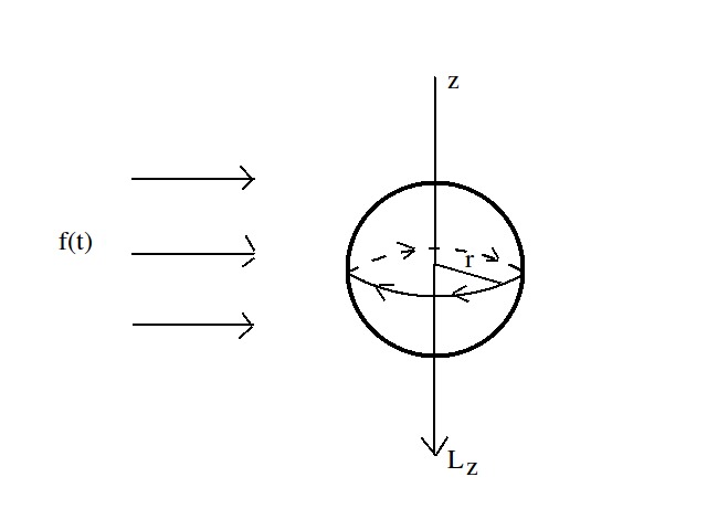
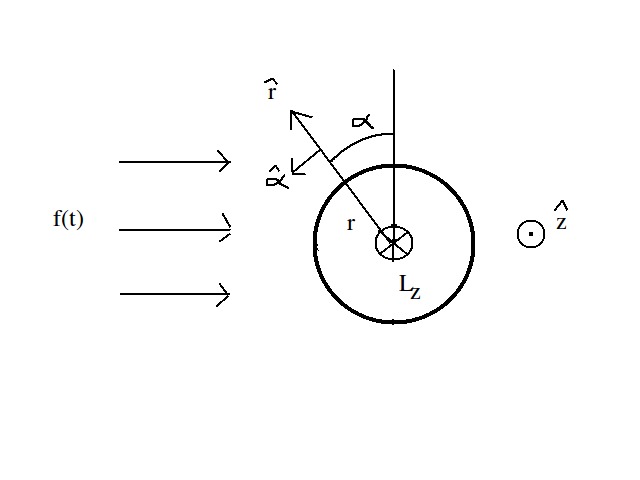
Figure 6: Left: Cartoon to schematic torque computation generated by an external forcing. Right: Azimuthal projection.

Using the fact that $\displaystyle\tau=\frac{dL}{dt}$, we have:

$$\ell_{z}=-\int r~{}f(t)\sin\alpha~{}dt$$ (3)

Looking at a given $r$ and $\alpha$ we obtain:

$$\ell_{z}=-r~{}\sin\alpha~{}\int f(t)dt$$ (4)

By definition $p=mv\Rightarrow\delta p=fdt$ and $\Delta p=\int\delta p$. Therefore:

$$\ell_{z}=-r~{}\sin\alpha~{}\Delta p$$ (5)

If we integrate over every $\alpha$, by symmetry the only contribution will be for $\alpha=\pi/2$

$$\ell_{z}=-r~{}\Delta p$$ (6)

It means that for an external contribution to the atmospherics winds, we need a non-zero net moment transfer.

But, is it enough? In principle, this seems to be difficult because by symmetry the only point that receive this contribution is the solar point which is a “point” of zero measure. In any case, if there is an external source of superrotation wind, it is necessary to show temporal and velocity scales, dispersion relation and waves propagation due this effect.

III.3.2 Temperature Gradients

As mentioned before, between day and night sides there exist strong gradients of temperature. In principle in the upper levels the gradient is smoother than in superficial levels, because superrotating winds tends to uniformise the temperature differences more efficiently than in the lower levels, where the winds are slower by an order of magnitude. (Durand-Manterola, 2010)

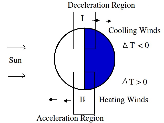
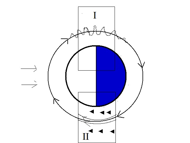
Figure 7: Left: Temperature gradients provocates two regions, Region I; where the winds are stopped, the morphology is corrugated clouds shape. In opposite, Region II; the winds are accelerated, corresponding to smooth clouds shape. Right: Cartoon of wind shape in each region.

III.3.3 Albedo Radiation

Venus is a slow rotating planet, and the day and night sides have a strong difference in their Albedo. The behaviour of the incident radiation on the planet can be approximated as a white body in the day side and like a black body in the nightside, see Figure 8. Chafin (2014) (Chafin, 2014) estimated this pressure gradient like

$$\tau=\int z~{}dF=\int z~{}P_{rad}~{}dA=\int_{0}^{r}z~{}P_{rad}~{}(2\sqrt{R^{2}-z^{2}})~{}dz=\frac{2}{3}P_{rad}~{}r^{3}$$ (7)

with $P_{rad}\propto 9\cdot 10^{-6}$Pa. He showed that this value is compatible with superrotating wind. 

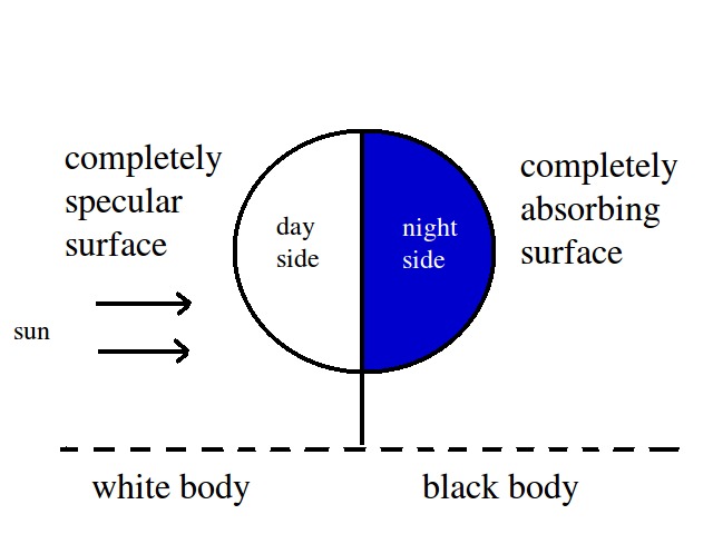
Figure 8: The Albedo difference between day side and night side generates a pressure gradient from day to night.

III.3.4 Durand Manterola’s hypothesis

Between altitudes in between 150 and 800km supersonic winds exist called transterminator flows. Considering again Fig 5, the external cell due to the influence of solar wind generates a photo-ionization pressure gradient. There two cells from day to night sides. However, the planet also slowly rotates. As shown in Fig 7 two regions can be defined:

• Region I: dusk zone; the external layer of the cell has a solidary speed respect to the rotation of the planet with velocity $v_{I}$.

• Region II: dawn zone; the external layer of the cell has an opposite speed respect to the rotation of the planet with velocity $v_{II}$.

In the night side, particularly in the anti-solar point, one can consider the mechanism in Fig 9. In this region $v_{I}=10V_{II}$ the contact of the two flows generates turbulence and a pressure gradient which creates waves transferring angular momentum in the retrograde sense, between external layers of Hadley cells and superrotating winds in the upper levels. This energy, according to Durand-Manterola (2010) has enough power to overcome viscosity losses and could explain superrotating winds.

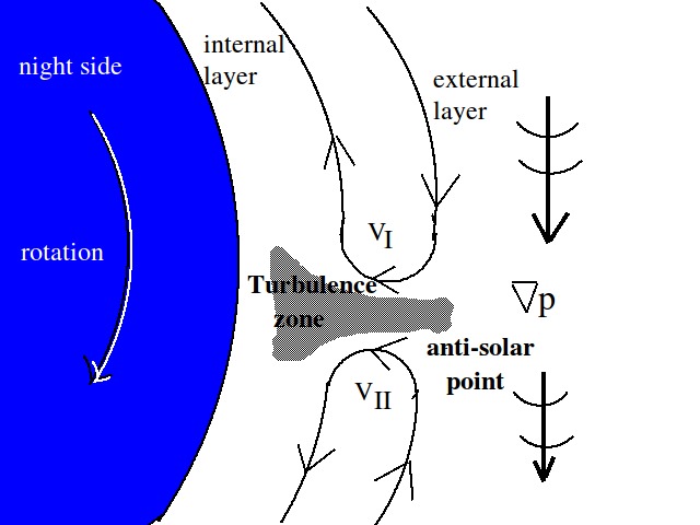
Figure 9: Presence of transterminator flows, in the anti-solar point could generate a transversal gradient of pressure which colaborates with the angular momentum of superrotating winds.

Durand-Manterola (2010) found that using the Darcy-Weisbach equation, two fluxes at different velocities generate turbulence and wave propagation, transferring energy between different atmospheric layers:

$$\delta P=f_{D}~{}\frac{L}{D}~{}\frac{1}{2}~{}\rho v^{2}$$ (8)

where $f_{D}$ is the friction, $D$ the pipe diameter, $L$ typical longitude.
They set an experiment with two water “pipes” falling off at different velocities (2m/s and 0.2m/s) and found wave propagation and a the generation of a net flow (velocity 0,63m/s) giving a net angular momentum. The basic scheme of the experiment is shown in Fig 10

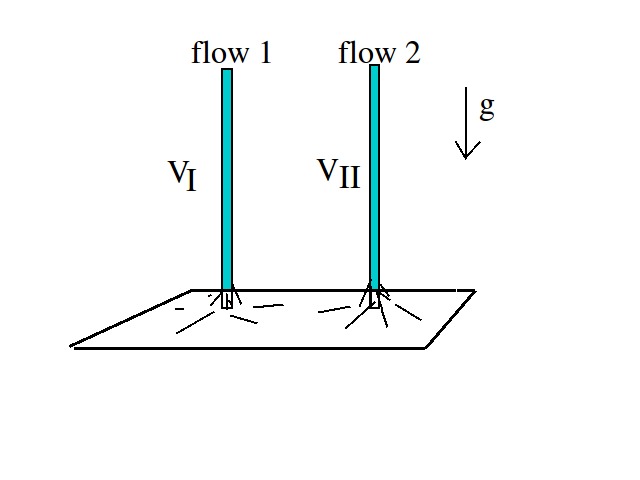
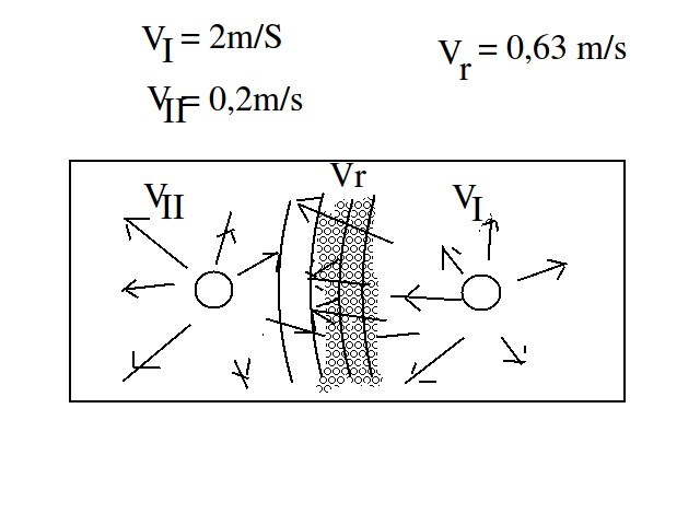
Figure 10: Cartoon of Durand-Manterola’s experiment which try to emulate the Fig 9. Left: in perspective. Right: azimuthal view.

IV Gravity waves

As mentioned above in the Gierasch mechanism the role of gravity waves is relevant to the generation of superrotation. For that reason, it is important to observe and measure their behaviour.

Gravity waves are wave disturbances in which buoyancy acts as the restoring force. These waves (internal gravity or buoyancy waves) abound in the stable density layering of the upper atmosphere. Their effects are visibly manifest in the curls of the clouds, in the moving skein-like and billow patterns of the clouds in the middle of the venusian atmosphere, and in the slowly shifting bands of the top part of the atmosphere. In terrestrial planets the characteristic of gravity waves are similar and its description is analogous to gravity waves in Earth, and since the seventies detailed studies exist about it, for example see Francis (1975) Francis (1975).

What produces them? These waves can be generated by disturbances in the lowest part of the atmosphere, for example, wind flow over mountain ranges and violent thunderstorms. Jet stream shear and solar radiation are other sources. An initial small amplitude in the lower atmosphere increases with height until the waves break in the mesosphere and lower thermosphere. Their wavelengths can range up to some hundreds of kilometers. Their periods ranging from a few minutes to days. Given the possible generation by flow over mountain ranges Piccialli et al. (2014), detailed works exist relating wave morphology and mapping of the planets, for example see Basilevsky (2003) Basilevsky and Head (2003).

Recent works, Fukuhara et al. (2017) Fukuhara et al. (2017), using the orbiter instrument Akatsuki suggest that bow shaped structures are the result of gravity waves generated in the lower atmosphere by mountain topography (around 10 km height), that propagate upwards. The authors modeled large scale gravity waves to be compared with observations supporting these assumptions. Although the dayside is well known, the nightside is not sufficiently observed. Peralta et al. (2017) Peralta et al. (2017) using results from the Venus Express mission report that stationary waves in the upper atmosphere in the nightside are slower than in the dayside hemisphere, imposing constraints to Venus general circulation models that do not predict such phenomena. Akatsuki and Venus Express observations will be important to elucidate the features in the upper clouds in the day and night sides.

V Simple Model

In this section we are going to show that superrotation speed solutions are possible in a stationary regime due a temperature gradient by the sun irradiation in a slowly rotating planet. If we consider a differential volume at given latitude and altitude, see Figure 11.

V.1 Basic equations

To explore the possibility to generate superrotating winds by the temperature gradient due to the solar irradiation over the atmosphere, we build a simplified model which has the following assumptions.

• Stationary wind regime.

• $2\pi$-periodicity condition in the solar point.

• Friction, radial and azimuthal velocities are negligible compared to $u_{\phi}$, the zonal wind velocity.

• We take the atmosphere as an ideal gas.

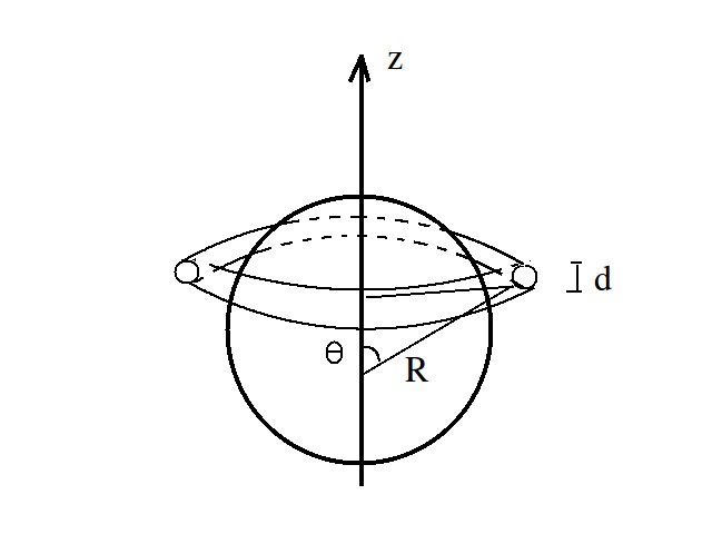
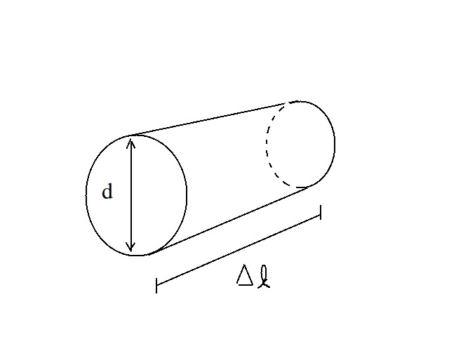
Figure 11: Cylindrical volume of diameter $d=\lambda_{abs}$, at radius $R$ and angle $\theta$ with dimensions $\delta Sup=\pi\lambda_{abs}\Delta\ell\Rightarrow\delta V=\frac{\pi\lambda_{abs}^{2}}{4}\Delta\ell$

The continuity equation is then:

$$\frac{\partial}{\partial\phi}(\rho u_{\phi})=0$$ (9)

Where $\rho$ is the mass density.

The dynamic equations are:

$$\frac{u_{\phi}}{r}\frac{\partial u_{\phi}}{\partial\phi}=-\frac{1}{\rho}\frac{\partial p}{\partial\phi}$$ (10)

where $r\sin\theta=R$, and

$$\frac{u_{\phi}^{2}}{2}=-\frac{1}{\rho}\frac{\partial p}{\partial r}-g_{r}$$ (11)

where $g_{r}$ is the radial gravity component. Also, the specific entropy $s$ equation is:

$$\rho\frac{u_{\phi}}{r}\frac{\partial s}{\partial\phi}=\frac{\dot{Q}}{T}$$ (12)

Where $\dot{Q}$ is the rate of absorbed or emitted heat per unit volume, and $T$ the temperature. Under the assumption of ideal gas and using the first principle of the thermodynamics:

$$\delta Q-\delta W=dU\Rightarrow T\delta S-p\delta V=nC_{v}dT$$ (13)

where $n$ is the number of mol and $R_{m}=0.082\ell\mathrm{{atm}/molK}$ we obtain:

$$\delta s=C_{v}~{}\frac{dT}{T}-R_{m}\frac{\delta\rho}{\rho}$$ (14)

Combining the energy equation with the entropy equation:

$$\frac{R_{m}T}{\rho}\frac{\partial\rho}{\partial\phi}=C_{v}\frac{\partial T}{\partial\phi}-\frac{r\dot{Q}}{\rho u_{\phi}}$$ (15)

Since $\delta p=R_{m}\rho dT+R_{m}T\delta\rho$ we have the equation for radial velocity:

$$\frac{1}{2}\frac{\partial u_{\phi}^{2}}{\partial\phi}=u_{\phi}\frac{\partial u_{\phi}}{\partial\phi}=-R_{m}\frac{\partial T}{\partial\phi}-R_{m}\frac{T}{\rho}\frac{\partial\rho}{\partial\phi}$$ (16)

Using the continuity equation, $R_{m}=C_{p}-C_{v}$ and constant $\rho u_{\phi}$, we have a balance equation like:

$${\frac{\partial}{\partial\phi}(C_{p}T+u_{\phi}^{2}/2)=\frac{r\dot{Q}}{\rho u_{\phi}}}$$ (17)

Also, $\dot{Q}$ is the balance between the albedo radiation, black-body emission and diffusivity:

$$\dot{Q}=\dot{Q}_{\odot}-\sigma T^{4}\frac{\delta Sup}{\delta V}+\frac{k}{r^{2}}\frac{\partial^{2}T}{\partial\phi^{2}}$$ (18)

Where

$$\dot{Q}_{\odot}=\left\{\begin{array}[c]{ll}\displaystyle\frac{I_{\odot}}{4}\frac{\delta Sup}{\delta V}~{}f_{abs}&\mathrm{{if}~{}~{}~{}\phi>\phi_{0}}\\ 0&\mathrm{{if}~{}~{}~{}\phi\leq\phi_{0}}\end{array}\right.$$

Considering an annular volume and neglecting the diffusion term, we have:

$${\dot{Q}=\frac{I_{\odot}}{\lambda_{abs}}sen\theta cos\phi~{}f_{abs}\Theta(cos\phi)-\frac{4\sigma}{\lambda_{abs}}(T^{4}-T_{ref}^{4})}$$

being:

• $f_{abs}$ an absorption factor related with Albedo which depends on the temperature and solar radiation.

• $\Theta(cos\phi)$ Heaviside function.

• $I_{\odot}$ solar radiative intensity.

• $\lambda_{abs}$ characteristic absorption scale.

• $T_{ref}$ is a reference temperature.

Using again the continuity equation in the expression for velocity we arrive at the following relation:

$$u_{\phi}+\frac{p}{\rho u_{\phi}}=cte$$ (19)

Finally, assuming ideal gas…

$$\frac{dT}{d\phi}=\frac{r\dot{Q}}{c_{p}\rho u_{\phi}}=\frac{r\dot{Q}}{c_{p}K}\sqrt{\frac{KR_{m}T}{p_{0}}},$$ (20)

where

$$K=\sqrt{\frac{pu_{\phi}^{2}}{R_{m}T}}$$ (21)

is the eigenvalue obtained by imposing a $2\pi$ periodic solution.

V.2 Numerical experiments

With the model developed in last section we took observed values of pressure and temperature as a function of altitude to evaluate wind speeds and compare with the observed ones.

According to our model, preserving the periodicity and fitting parameters adequately, we obtained wind velocity profiles in the range between 50 and 80 Km similar to those observed. In this way we obtained each profile for a given latitude and altitude for the whole planet. We made this for Venus and Titan.

V.2.1 Venus

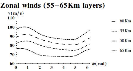
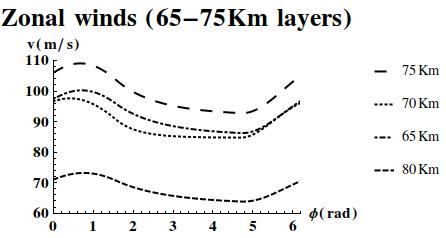
Figure 12: Zonal winds at different altitudes versus latitude, $\phi=0$ midday, $\phi=\pi$ midnight. Left: Between 55 and 65 Km layers. Right: Between 65 and 75 Km layers.

From Figure 12 we can see that the speed is lower in the interval $\{\pi/3;5\pi/3\}$ corresponding to the migration from the solar point to the nightside $\{\pi/2;3\pi/2\}$. Later, when the wind returns to the dayside the speed increases.

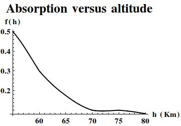
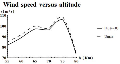
Figure 13: Left: absorption coefficients used for numerical fitting. Right: Comparison between speed wind at $\phi=0$ and maximum speed for the layers in the range 50-80km height

Fig 13 shows the absorption coefficients as a function of altitude used for numerical fitting (left) and the speed of wind in the solar point comparing with the maximal speed (right). We can see for one side that it which is consistent with the fact that the clouds layer increases the absorption and by another side the difference in velocity in each layers are not greater than a $10\%$.

V.2.2 Titan

In the same way we made the fit taking atmospheric values of Titan, in a qualitative way, we observed a similar behaviour to the Venusian case. Comparing with Venus the difference in the fluctuations in speed are lower due essentially by the solar irradiance. Qualitatively, the values are similar to the observed ones indicating that the influence of Saturn it seems not relevant to the wind dynamics for our model.

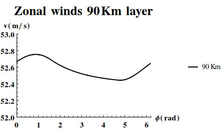
Figure 14: Zonal winds at different altitudes versus latitude, $\phi=0$ midday, $\phi=\pi$ midnight. Left: Between 60 and 125 Km layers. Right: More detailed zonal wind at 90Km layer.

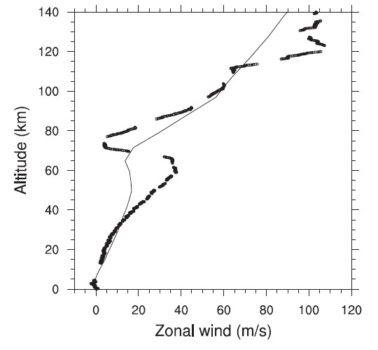
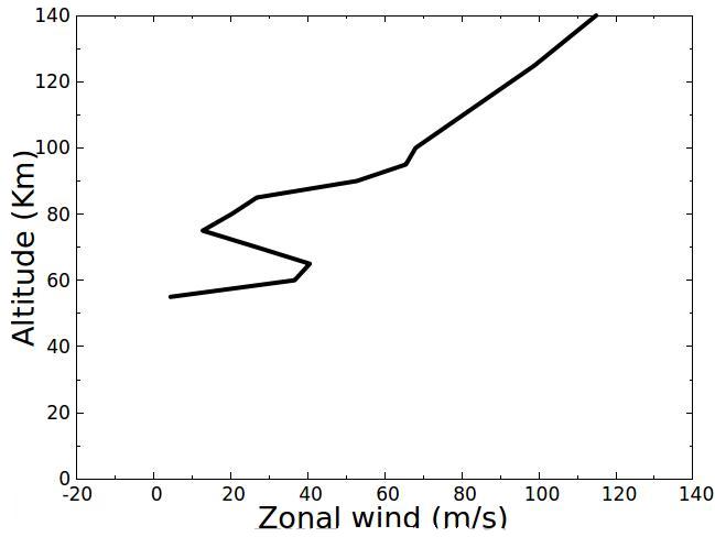
Figure 15: Left: observed values (Bird et al Bird et al. (2005)). Right: values obtained with our model.

VI Concluding remarks an outlook

In this paper we have reviewed and analyzed the problem of superrotation on Venus in light of the interest that the latest data have produced in the scientific community. These data introduce a clear indication that traditional theoretical approaches have to be modified in some way. Although the model introduced here is capable of reproducing the general behavior of the wind in super rotation (at least in the layers of interest), under the assumptions of slow rotating planet and stationary regime due by heat balance is stablished. The model indicates that the main source to supply superrotation is the solar irradiance. However, the problem of the generation of superrotation remains an enigma. Another problem is described in Fukuhara et al. (2017) that is interesting from the theoretical point of view because it presents the challenge of constructing a formulation that gives a global description of the dynamics of the Venusian atmosphere. The other question is whether a relationship between the phenomenon of superrotation on different planets and satellites certainly exists.

VII Acknowledgements

We gratefully acknowledge to the Departamento de Física (FCEyN, UBA) and Instituto de Física del Plasma (CONICET-UBA), FM and DC are also grateful to the Consejo Nacional de Investigaciones Científicas y Técnicas, CV is also grateful to the Instituto de Ciencias (UNGS) and DC is also grateful to the Bogoliubov Laboratory of Theoretical Physics for their institutional support.

References

- Peralta et al. (2014) J. Peralta, T. Imamura, P. L. Read, D. Luz, A. Piccialli, and M. A. López-Valverde, ApJ Series 213, 18 (2014).
- Gierasch et al. (1997) P. J. Gierasch, R. M. Goody, R. E. Young, D. Crisp, C. Edwards, R. Kahn, D. Rider, A. del Genio, R. Greeley, A. Hou, C. B. Leovy, D. McCleese, and M. Newman, in Venus II: Geology, Geophysics, Atmosphere, and Solar Wind Environment, edited by S. W. Bougher, D. M. Hunten, and R. J. Phillips (1997) p. 459.
- Bougher et al. (1997) S. W. Bougher, M. J. Alexander, and H. G. Mayr, in Venus II: Geology, Geophysics, Atmosphere, and Solar Wind Environment, edited by S. W. Bougher, D. M. Hunten, and R. J. Phillips (1997) p. 259.
- Peralta Calvillo (2008) J. Peralta Calvillo, Vientos, Turbulencia y ondas en las nubes de Venus, Ph.D. thesis, Escuela Superior de Ingeniería. Departamento de Física Aplicada I, UPV (2008).
- Mahieux et al. (2012) A. Mahieux, A. C. Vandaele, S. Robert, V. Wilquet, R. Drummond, F. Montmessin, and J. L. Bertaux, Journal of Geophysical Research (Planets) 117, E07001 (2012).
- Dolginov et al. (1968) S. Dolginov, E. Yeroshenko, and L. Zhuzgov, Kosmich. Issled. (1968).
- Dolginov et al. (1969) S. S. Dolginov, E. G. Eroshenko, and L. Davis, Kosmicheskie Issledovaniia 7, 747 (1969).
- Dolginov and et al. (1972) S. Dolginov and et al., Nauka, Moscow (1972).
- Bridge et al. (1967) H. S. Bridge, A. J. Lazarus, C. W. Snyder, E. J. Smith, L. Davis, Jr., P. J. Coleman, Jr., and D. E. Jones, Science 158, 1669 (1967).
- Dolginov et al. (1973a) S. S. Dolginov, E. G. Eroshenko, and L. N. Zhuzgov, Soviet Physics Doklady 17, 1117 (1973a).
- Dolginov et al. (1973b) S. S. Dolginov, Y. G. Yeroshenko, and L. N. Zhuzgov, jgr 78, 4779 (1973b).
- Spreiter and Alksne (1970) J. R. Spreiter and A. Y. Alksne, Annual Review of Fluid Mechanics 2, 313 (1970).
- Spreiter et al. (1970) J. R. Spreiter, A. L. Summers, and A. W. Rizzi, planss 18, 1281 (1970).
- Cloutier and Daniell (1973) P. A. Cloutier and R. E. Daniell, planss 21, 463 (1973).
- Cloutier et al. (1974) P. A. Cloutier, R. E. Daniell, and D. M. Butler, planss 22, 967 (1974).
- Bauer and Hartle (1973) S. J. Bauer and R. E. Hartle, jgr 78, 3169 (1973).
- Smith et al. (1965) E. J. Smith, L. Davis, Jr., P. J. Coleman, Jr., and D. E. Jones, Science 149, 1241 (1965).
- Smith (1969) E. J. Smith, Adv. Astronaut. Sci. (1969).
- Gringauz et al. (1968) K. I. Gringauz, V. V. Bezrukikh, G. Volkov, L. Musatov, and T. Breus, Kosmicheskie Issledovaniia 5, 411 (1968).
- Gringauz et al. (1970) K. I. Gringauz, V. V. Bezrukikh, G. I. Volkov, L. S. Musatov, and T. K. Breus, Kosmicheskie Issledovaniia 8, 431 (1970).
- Gringauz et al. (1973) K. I. Gringauz, V. V. Bezrukikh, G. I. Volkov, T. K. Breus, I. S. Musatov, L. P. Havkin, and G. P. Sloutchonkov, icarus 18, 54 (1973).
- Gringauz and et al. (1972) K. I. Gringauz and et al., Kosmicheskie Issledovaniia 10, 462 (1972).
- Gringauz and et al. (1973) K. I. Gringauz and et al., Kosmicheskie Issledovaniia 11, 743 (1973).
- Vaisberg and Bogdanov (1974) O. L. Vaisberg and A. V. Bogdanov, Kosmicheskie Issledovaniia 12, 279 (1974).
- Whitten and Colin (1974) R. C. Whitten and L. Colin, Reviews of Geophysics and Space Physics 12, 155 (1974).
- Herman et al. (1971) J. R. Herman, R. E. Hartle, and S. J. Bauer, planss 19, 443 (1971).
- Izakov (2001) M. Izakov, Astronomicheskii Vestnik (2001).
- Gierasch (1975) P. J. Gierasch, Journal of Atmospheric Sciences 32, 1038 (1975).
- del Genio and Suozzo (1987) A. D. del Genio and R. J. Suozzo, Journal of Atmospheric Sciences 44, 973 (1987).
- Yamamoto and Takahashi (2003) M. Yamamoto and M. Takahashi, Journal of Atmospheric Sciences 60, 561 (2003).
- Durand-Manterola (2010) H. J. Durand-Manterola, ArXiv e-prints (2010), arXiv:1005.3488 [astro-ph.EP] .
- Chafin (2014) C. Chafin, ArXiv e-prints (2014), arXiv:1406.0116 [astro-ph.EP] .
- Francis (1975) S. H. Francis, Journal of Atmospheric and Terrestrial Physics 37, 1011 (1975).
- Piccialli et al. (2014) A. Piccialli, D. V. Titov, A. Sanchez-Lavega, J. Peralta, O. Shalygina, W. J. Markiewicz, and H. Svedhem, icarus 227, 94 (2014).
- Basilevsky and Head (2003) A. T. Basilevsky and J. W. Head, Reports on Progress in Physics 66, 1699 (2003).
- Fukuhara et al. (2017) T. Fukuhara, M. Futaguchi, G. Hashimoto, T. Horinouchi, T. Imamura, N. Iwagaimi, T. Kouyama, S. Murakami, M. Nakamura, K. Ogohara, M. Sato, T. Sato, M. Suzuki, M. Taguchi, S. Takagi, M. Ueno, S. Watanabe, M. Yamada, and A. Yamazaki, Nature Geosciences 10, 85 (2017).
- Peralta et al. (2017) J. Peralta, R. Hueso, A. Sánchez-Lavega, Y. J. Lee, A. G. Muñoz, T. Kouyama, H. Sagawa, T. M. Sato, G. Piccioni, S. Tellmann, T. Imamura, and T. Satoh, Nature Astronomy 1, 0187 (2017), arXiv:1707.07796 [astro-ph.EP] .
- Bird et al. (2005) M. K. Bird, M. Allison, S. W. Asmar, D. H. Atkinson, I. M. Avruch, R. Dutta-Roy, Y. Dzierma, P. Edenhofer, W. M. Folkner, L. I. Gurvits, D. V. Johnston, D. Plettemeier, S. V. Pogrebenko, R. A. Preston, and G. L. Tyler, Nature (London) 438, 800 (2005).