Rapid Near-Neighbor Interaction of High-dimensional Data via Hierarchical Clustering

Abstract.

Calculation of near-neighbor interactions among high dimensional, irregularly distributed data points is a fundamental task to many graph-based or kernel-based machine learning algorithms and applications. Such calculations, involving large, sparse interaction matrices, expose the limitation of conventional data-and-computation reordering techniques for improving space and time locality on modern computer memory hierarchies. We introduce a novel method for obtaining a matrix permutation that renders a desirable sparsity profile. The method is distinguished by the guiding principle to obtain a profile that is block-sparse with dense blocks. Our profile model and measure capture the essential properties affecting space and time locality, and permit variation in sparsity profile without imposing a restriction to a fixed pattern. The second distinction lies in an efficient algorithm for obtaining a desirable profile, via exploring and exploiting multi-scale cluster structure hidden in but intrinsic to the data. The algorithm accomplishes its task with key components for lower-dimensional embedding with data-specific principal feature axes, hierarchical data clustering, multi-level matrix compression storage, and multi-level interaction computations. We provide experimental results from case studies with two important data analysis algorithms. The resulting performance is remarkably comparable to the BLAS performance for the best-case interaction governed by a regularly banded matrix with the same sparsity.

1. Introduction

We introduce a new method for improving data locality, and thereby performance on modern computer architectures, for iterative near-neighbor interaction computations among scattered data points in a high-dimensional feature space. Such interactions are a fundamental computational task in several high-impact and frequently used algorithms for exploratory data analysis or machine learning applications. Among others, they arise in the mean-shift (MS) (Fukunaga and Hostetler, 1975; Comaniciu and Meer, 2002), stochastic neighbor embedding (SNE) (Hinton and Roweis, 2003), and t-student stochastic neighbor embedding (t-SNE) (Maaten and Hinton, 2008; van der Maaten, 2014) algorithms. Iterative interactions are becoming a speed bottleneck as the data sets are growing bigger.

We give a simple description of iterative interaction computations. Denote by $\mathcal{S}=\mathopen{}\mathclose{{}\left\{s_{j}\,\middle|\,j=1,\ldots,N}\right\}$ and $\mathcal{T}=\mathopen{}\mathclose{{}\left\{t_{i\phantom{j}}\!\!\,\middle|\,i=1,\ldots,M}\right\}$ the source (or reference) and the target (or response) point set, respectively, in a $D$-dimensional feature space, $\mathbb{R}^{D}$. The sources may be the corpus or training data in a stationary setting. The targets may correspond to query or test data. Very often, feature dimensionality is high and the data sets are big. For instance, the feature dimension is $49$ with $7\!\times\!7$ patch features, as often used in image analysis methods, and it can be as high as ${\sim}1000$ with GIST descriptors (Oliva and Torralba, 2001). The number of data points can be in the order of millions or even billions.

At iteration step $\kappa$, we denote by $\boldsymbol{\mathbf{x}}_{\kappa}=[x_{\kappa}(s_{j})]$ the charge (reference) vector defined on the source set and governed by the charge function $x$. We denote by $\boldsymbol{\mathbf{y}}_{\kappa}$ the potential (response) vector at the target points due to the impact of the charge $\boldsymbol{\mathbf{x}}_{\kappa}$. In a stationary setting, the near-neighbor interaction computation is dominated by a matrix-vector multiplication $\boldsymbol{\mathbf{y}}_{\kappa}=\boldsymbol{\mathbf{A}}\boldsymbol{\mathbf{x}}_{\kappa}$, where $\boldsymbol{\mathbf{A}}$ is the near-neighbor interaction matrix,

(1) $$\alpha_{ij}=f(t_{i},s_{j})\quad\text{iff}\quad s_{j}\in\operatorname{near-neighbors}(t_{i}), 1\leq i\leq M$$

and $f$ is the kernel function governing the source-target interaction. Near-neighbor relationships are determined by a given distance measure in the feature space, $\mathbb{R}^{D}$. The matrix columns and rows correspond to the source and target points, respectively. We are concerned primarily with the non-stationary setting, where one or both sets may migrate in $\mathbb{R}^{D}$ during the course of iterative interactions. While the data coordinates change, the near-neighbor interaction matrix is updated accordingly, from $\boldsymbol{\mathbf{A}}_{\kappa-1}$ to $\boldsymbol{\mathbf{A}}_{\kappa}$. For convenience, we assume $M=N$ from now on, unless stated otherwise.

The interaction matrix $\boldsymbol{\mathbf{A}}$ is related to a bipartite graph, with edges between the source vertex set $\mathcal{S}$ and the target vertex set $\mathcal{T}$. Often, the number of neighbors for each target point is specified to a predetermined, modest parameter value $k\ll N$. The matrix profile corresponds to the $k$-nearest neighbors ($k$NN) graph; it is sparse, and not necessarily symmetric. Near-neighbor interactions include those in traditional sparse matrix computations, such as Laplacian diffusion in a low-dimensional space-time coordinate space, over points on a regular or irregular mesh.

Near-neighbor interactions among large data points in a high-dimensional feature space tend to suffer from the widening gap between processor speed and memory speed (Rixner et al., 2000). Furthermore, they expose the limitations of conventional techniques for improving data locality via data-computation reordering, at the system level and/or at the application algorithm level. Locality improvement at the system level relies on a particular program instantiation of an application algorithm (Mellor-Crummey et al., 2001). At the application algorithm level, it has a larger scope to alter program instantiation and memory access footprint (George et al., 1986; Barnard et al., 1995; Mellor-Crummey et al., 2001); the latter, however, is challenged by high dimensionality.

When the feature dimension $D$ is high, then $N\ll 2^{D}$. This relationship between data size and dimension speaks plainly to the fact that the data points are sparsely distributed in the feature space, unlike the points on, and well-connected by, a low-dimensional mesh. By conventional matrix ordering techniques, as we shall show shortly, the near-neighbor interaction matrix remains highly sparse within an optimal envelope; for conventional sparsity profile types, see (Mellor-Crummey et al., 2001; Barnard et al., 1995) and the references therein. By the minimum bandwidth envelope, for example, the bandwidth in a row is typically much larger than the number of near neighbors, i.e., the number of non-zero elements in the row. This phenomenon may be viewed as a shadow of the so-called curse of dimensionality. We introduce our method to step away from this shadow.

We explore the potential, at the algorithm level, to further utilize processor speed and circumvent memory access latency due to scattered referencing among high-dimensional irregular data, by means of exploring and exploiting multi-scale cluster structure that is hidden in but intrinsic to the data set. The method itself is data adaptive. There are two main aspects to the novelty of our approach.

The first novelty lies in the principled pursuit of a matrix profile that is block-sparse with dense blocks. The guiding principle suggests that neighboring, interacting elements should be clustered as densely as possible. In an ideal ordering, the sparsity profile has at least a two-level structure: very sparse in nonzero sub-matrices (blocks); much denser within in each nonzero block. We present in Sections 2.1 and 2.2 a descriptive measure of what we term the patch density of a matrix, for quantitative evaluation of and comparison between particular profiles. The profile model and measure reflect and capture essential properties affecting space and time locality for sparse matrix-vector multiplications.

The second contribution lies in a new algorithm for efficiently locating an ordering that renders a near-optimal matrix profile, based on intrinsic multi-scale relationships among the data. The algorithm is composed of key components for lower-dimensional embedding with data-specific principal feature axes, hierarchical data clustering, multi-level matrix compression storage, and multi-level interaction computations. We describe the algorithm in Section 2.4.

We assess the efficacy of our method with two case studies, involving the applications of the MS and t-SNE algorithms to large, high-dimensional data sets. We describe the case studies briefly in Section 3. Experimental results are presented in Section 4. Comparisons between different ordering schemes are made with respect to patch density measure and throughput performance, besides visual inspection and comparison of the sparsity profiles. The results demonstrate 1 superior performance to that of state-of-the-art ordering methods at the algorithm level; and 2 remarkable consistency between visual profiles and patch density measure on the one side and execution time and throughput on the other. We conclude the paper with a brief overview additional remarks and a brief overview of related work in Section 5.

2. Maximum patch-density ordering

In this section, we first introduce our guiding principle for identifying matrix sparsity profiles that are conducive to better space and time locality for near-neighbor interactions among data points in a high-dimensional space. We materialize the principle into a quantitative measure of the sparse profile of any given ordering and its maximal value among all orderings. We term this measure the patch density score. An optimal matrix ordering renders the maximal patch density score. Then, we present an efficient and effective algorithm for attaining a near-optimal matrix ordering.

2.1. Block-sparse with dense blocks

Given a sparse matrix, we seek row and column re-orderings such that the sparsity profile is block-sparse with dense blocks. We illustrate first in Fig. 1 four sparsity profiles of the same matrix as per four different orderings; their relationship to one another is explained in the caption. After specifying what we mean by block sparsity and dense blocks, we argue that the two properties are integral to each other, and that they are essential to relating data locality to matrix sparsity profile and further characterizing this relationship.

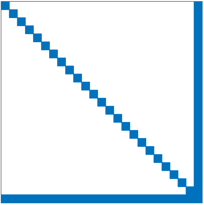
(a) $\operatorname{\beta}\approx 0.20$
(a) $\gamma=21.0$

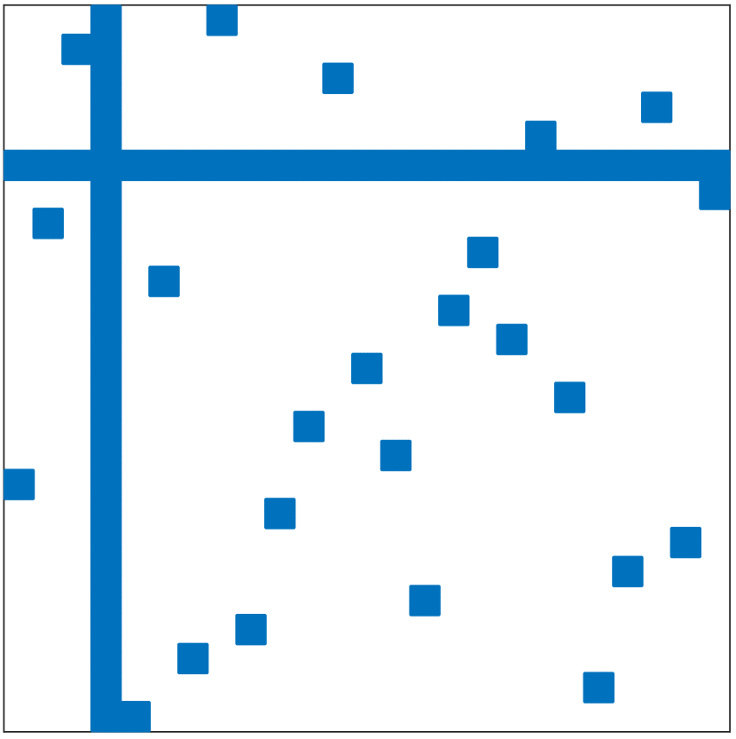
(b) $\operatorname{\beta}\approx 0.20$
(b) $\gamma=20.9$

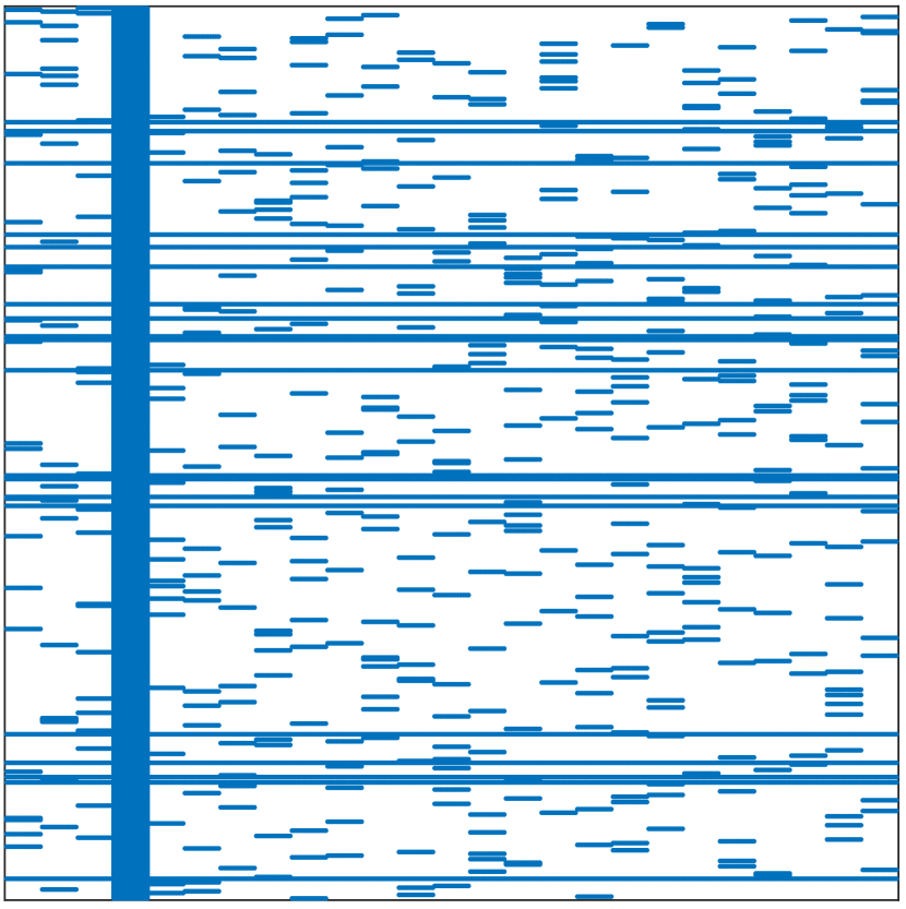
(c) $\operatorname{\beta}\geq 0.05$
(c) $\mspace{2.0mu}\gamma=10.5$

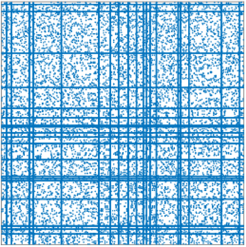
(d) $\operatorname{\beta}\geq 0.01$
(d) $\mspace{2.0mu}\gamma=4.5$

Figure 1. Sparsity profiles of the same $500\times 500$ matrix in four different orderings: (a) Block arrowhead with full $20\times 20$ blocks; (b) obtained from (a) with a random permutation among the block rows and columns; (c) obtained from (b) with a random permutation among the rows; and (d) obtained from (c) with a random permutation among the columns. Patch density is maximal for (a) and (b), the best case. It is reduced for (c), and further dropped for (d), the base case. The proposed patch density measure $\operatorname{\beta}$ and numerical density estimate $\gamma$, defined in (2) and (4), respectively, are shown for each ordering. The $\gamma$-scores (evaluated using $\sigma=10$) correlate well with the $\operatorname{\beta}$-scores.

In what follows, we denote by $\operatorname{nnz}\mathopen{}\mathclose{{}\left(\boldsymbol{\mathbf{A}}}\right)$ the total number of nonzero elements in a near-neighbor interaction matrix $\boldsymbol{\mathbf{A}}$. With $k$NN interaction in particular, $\operatorname{nnz}\mathopen{}\mathclose{{}\left(\boldsymbol{\mathbf{A}}}\right)=kN$. Denote by $\operatorname{area}(\boldsymbol{\mathbf{A}})$ the product of the number of rows and the number of columns, i.e., the total number of elements in $\boldsymbol{\mathbf{A}}$.

Dense blocks

Assume that the matrix in a certain ordering has a relatively denser sub-matrix, or simply block $\boldsymbol{\mathbf{B}}$, such as those in Figs. 1(a) and 1(b). By “relatively denser,” we mean that the ratio $\operatorname{nnz}\mathopen{}\mathclose{{}\left(\boldsymbol{\mathbf{B}}}\right)/\!\operatorname{area}(\boldsymbol{\mathbf{B}})$ is significantly higher than $\operatorname{nnz}\mathopen{}\mathclose{{}\left(\boldsymbol{\mathbf{A}}}\right)/\!\operatorname{area}(\boldsymbol{\mathbf{A}})$. When $\boldsymbol{\mathbf{A}}$ corresponds to a bipartite graph between the entire source and target data sets, block $\boldsymbol{\mathbf{B}}$ corresponds to a bipartite sub-graph with a cluster of target points sharing many of their neighbors in a cluster of source points. The density of $\boldsymbol{\mathbf{B}}$ may get close to $1$, despite the sparsity of $\boldsymbol{\mathbf{A}}$. For matrix-vector multiplication, such a dense block implies good locality in reading the charge sub-vector over the source cluster as well as good locality in writing to the response sub-vector over the target cluster, provided that the charge and response vectors are placed in memory according to the cluster structure.

Block sparsity

The nonzero blocks need not have the same size. By “block-sparse,” we mean that the dense blocks are sparsely distributed, i.e., the number of blocks is far smaller than $\operatorname{nnz}\mathopen{}\mathclose{{}\left(\boldsymbol{\mathbf{A}}}\right)$. In the trivial and extremely degenerate case, there are exactly $\operatorname{nnz}\mathopen{}\mathclose{{}\left(\boldsymbol{\mathbf{A}}}\right)$ nonzero blocks: a $1\!\times\!1$ block for each nonzero element. Next to this trivial extreme is the case where there are $\operatorname{nnz}\mathopen{}\mathclose{{}\left(\boldsymbol{\mathbf{A}}}\right)/c$ small blocks scattered throughout the matrix, for some small number $c$ which reflects the average size of the nonzero but small blocks. The block-sparsity condition discourages such degenerate cases.

Discussion

The principled sparsity profile model has two important consequences. The first one may be subtle. The model admits variations in matrix profiles, without imposing a fixed profile pattern. For instance, the profiles in Figs. 1(a) and 1(b) are considered equivalent in principle. This principled equivalence in sparsity profiles unifies several previously existing profile patterns. Particularly, the block-sparse profile of an arrowhead shape in Fig. 1(a) is in principle as good as its banded counterpart with the same number of nonzero elements.

Secondly, our principled sparsity profile is at the level of global matrix reordering. It applies naturally to the profiles of blocks, and hence leads to a hierarchical sparsity profile.

These properties make the model adaptive in practical computation to architecture specific performance tuning and/or to application specific customization in order to exploit additional structure.

2.2. Profile measure and optimal ordering

We have established a concrete measure of the sparsity profile of a matrix $\boldsymbol{\mathbf{A}}$ in any particular ordering. The measure favors sparsity profiles that match the block-sparse with dense blocks principle. For convenience in description, we introduce the concept of a patch covering of the nonzero elements in $\boldsymbol{\mathbf{A}}$. A patch covering is a set of non-overlapping blocks (patches) $\mathopen{}\mathclose{{}\left\{\boldsymbol{\mathbf{B}}_{\ell}}\right\}$ such that every nonzero element of $\boldsymbol{\mathbf{A}}$ lies within a patch in the covering. The covering size is $\mathopen{}\mathclose{{}\left|\mathopen{}\mathclose{{}\left\{\boldsymbol{\mathbf{B}}_{\ell}}\right\}}\right|$, the number of patches in $\mathopen{}\mathclose{{}\left\{\boldsymbol{\mathbf{B}}_{\ell}}\right\}$. The covering area is $\operatorname{area}(\mathopen{}\mathclose{{}\left\{\boldsymbol{\mathbf{B}}_{\ell}}\right\})=\sum_{\ell=1}^{\mathopen{}\mathclose{{}\left|\mathopen{}\mathclose{{}\left\{\boldsymbol{\mathbf{B}}_{\ell}}\right\}}\right|}\operatorname{area}(\boldsymbol{\mathbf{B}}_{\ell})$. The ratio $\operatorname{nnz}\mathopen{}\mathclose{{}\left(\boldsymbol{\mathbf{A}}}\right)/\!\operatorname{area}(\mathopen{}\mathclose{{}\left\{\boldsymbol{\mathbf{B}}_{\ell}}\right\})$ is the average density of the nonzero elements over the covering area. Let $\mathcal{P\!C}(\boldsymbol{\mathbf{A}})$ be the set of all possible patch coverings of $\boldsymbol{\mathbf{A}}$ in a particular ordering. Taking into account the block-sparse condition, which entails that the covering size be made as small as possible, we define the patch (covering) density measure as

(2) $$\operatorname{\beta}\mathopen{}\mathclose{{}\left(\boldsymbol{\mathbf{A}}}\right)=\max_{\mathopen{}\mathclose{{}\left\{\boldsymbol{\mathbf{B}}_{\ell}}\right\}\in\mathcal{P\!C}(\boldsymbol{\mathbf{A}})}\frac{1}{\mathopen{}\mathclose{{}\left|\mathopen{}\mathclose{{}\left\{\boldsymbol{\mathbf{B}}_{\ell}}\right\}}\right|}\frac{\operatorname{nnz}\mathopen{}\mathclose{{}\left(\boldsymbol{\mathbf{A}}}\right)}{\operatorname{area}(\mathopen{}\mathclose{{}\left\{\boldsymbol{\mathbf{B}}_{\ell}}\right\})}.$$

The best patch covering reaches the measure $\beta(\boldsymbol{\mathbf{A}})$, which is specific to any particular matrix ordering in rows and columns. We now define the optimal matrix row-column orderings as

(3) $$\mathopen{}\mathclose{{}\left(\boldsymbol{\mathbf{\pi}}_{\text{t}},\boldsymbol{\mathbf{\pi}}_{\text{s}}}\right)^{*}=\operatorname*{arg\mspace{2.0mu}max}_{(\boldsymbol{\mathbf{\pi}}_{\text{t}},\boldsymbol{\mathbf{\pi}}_{\text{s}})}\operatorname{\beta}\mathopen{}\mathclose{{}\left(\boldsymbol{\mathbf{A}}(\boldsymbol{\mathbf{\pi}}_{\text{t}},\boldsymbol{\mathbf{\pi}}_{\text{s}})}\right),$$

where $\boldsymbol{\mathbf{\pi}}_{\text{s}}$ and $\boldsymbol{\mathbf{\pi}}_{\text{t}}$ are permutations among columns (sources) and rows (targets), respectively.

Following the principle elaborated in Section 2.1, the patch density measure (2) relates to several existing profile patterns and measures used in sparse matrix computation. Limited by the manuscript length, we provide only a very simplified connection. With the same matrix size and number of nonzero elements, and the same number of dense blocks of equal size, block sparsity profiles with an arrowhead pattern, banded pattern, or any other pattern, reach to the same and maximal patch density score. This principled equivalence among such patterns amounts to a unification of them at the level of dense blocks, which correspond to cluster-cluster interactions and can be translated to space and time locality during matrix-vector multiplications and other operations.

The patch density score of (2) may be normalized by, say, the score for a block-tridiagonal matrix with the same size and number of nonzero elements. This is not necessary, however, because such normalization does not alter the optimization of (3).

2.3. Numerical measure estimate

The patch (covering) density measure $\operatorname{\beta}(\boldsymbol{\mathbf{A}})$ of (2) is in a combinatorial expression. Computation of the ordering-specific measure itself is NP-hard, let alone the search by (3) for the ordering with maximal patch density. We present in this section a relaxed and differential expression to get a numerical estimate of the $\beta$-score.

A relaxation shall be based on our profile principle as well as on the relationship (1) between the placement of nonzero elements in the matrix and the underlying near-neighbor relationships among the data points. Denote by $\mathcal{I}_{\text{nz}}(\boldsymbol{\mathbf{A}})$ the set of indices for the nonzero elements of $\boldsymbol{\mathbf{A}}$, $\mathcal{I}_{\text{nz}}(\boldsymbol{\mathbf{A}})=\mathopen{}\mathclose{{}\left\{(i,j)\,\middle|\,\alpha_{ij}\neq 0}\right\}$. This set represents the placement of the nonzero elements in the matrix by a particular ordering. Among many possible ways to relax the $\operatorname{\beta}$-score, we use the following $\gamma$-score,

(4) $$\gamma\mathopen{}\mathclose{{}\left(\boldsymbol{\mathbf{A}};\sigma}\right)=\frac{1}{\sigma\operatorname{nnz}\mathopen{}\mathclose{{}\left(\boldsymbol{\mathbf{A}}}\right)}\sum_{\boldsymbol{\mathbf{p}},\boldsymbol{\mathbf{q}}\in\mathcal{I}_{\text{nz}}(\boldsymbol{\mathbf{A}})}\exp\mathopen{}\mathclose{{}\left\{-\frac{\mathopen{}\mathclose{{}\left\|\boldsymbol{\mathbf{p}}-\boldsymbol{\mathbf{q}}}\right\|_{2}^{2}}{\sigma^{2}}}\right\},$$

where $\sigma$ is a scale parameter. The Gaussian function is defined over $\mathcal{I}_{\text{nz}}(\boldsymbol{\mathbf{A}})\times\mathcal{I}_{\text{nz}}(\boldsymbol{\mathbf{A}})$. A peak in the Gaussian function corresponds to a dense block in the matrix, where the block size is regulated by $\sigma$. All dense blocks do not necessarily have the same size, depending on whether the data points are clustered densely or loosely. In other words, the essential properties of the best patch covering in the combinatorial description are captured by the Gaussian function with smooth connections between interacting points and interacting point clusters.

By empirical tests we have carried out, the $\gamma$-score varies monotonically with the patch density score over the orderings used in the tests. See for instance the $\operatorname{\beta}$-scores and the $\gamma$-scores for the sparsity profiles in Fig. 1. We show also in Fig. 2 the sparse profiles of two real-data interaction matrices under different orderings, including the ordering by our algorithm, presented in the following section; the $\gamma$-score for each one is listed in Table 1.

SIFT

GIST

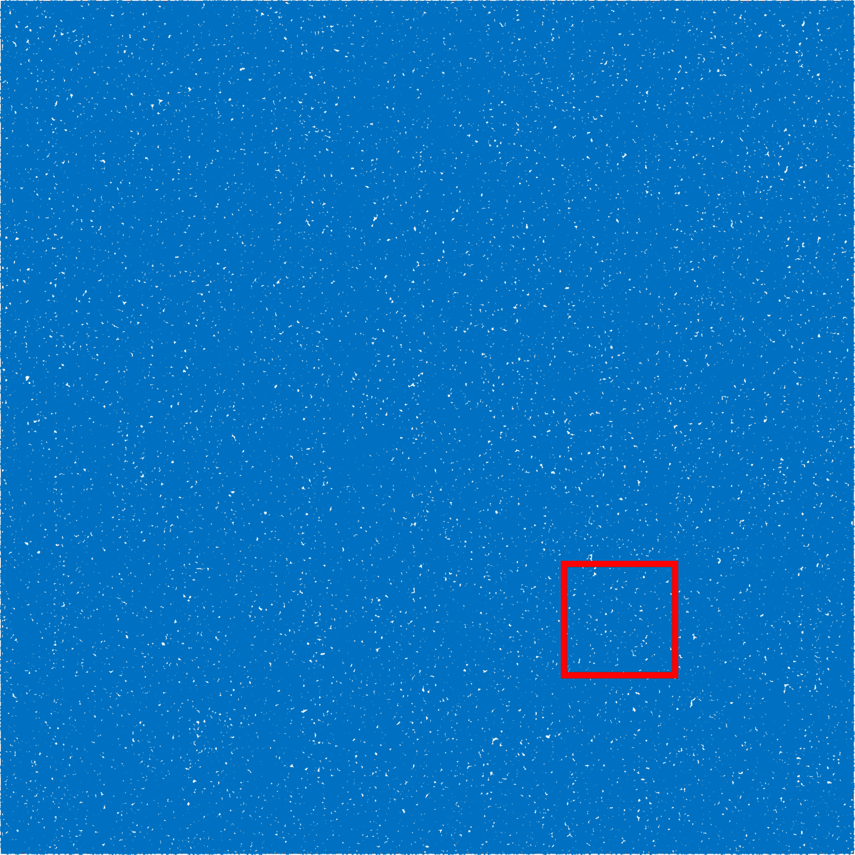
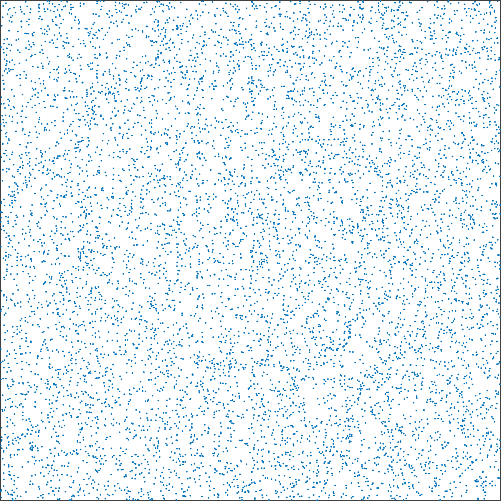
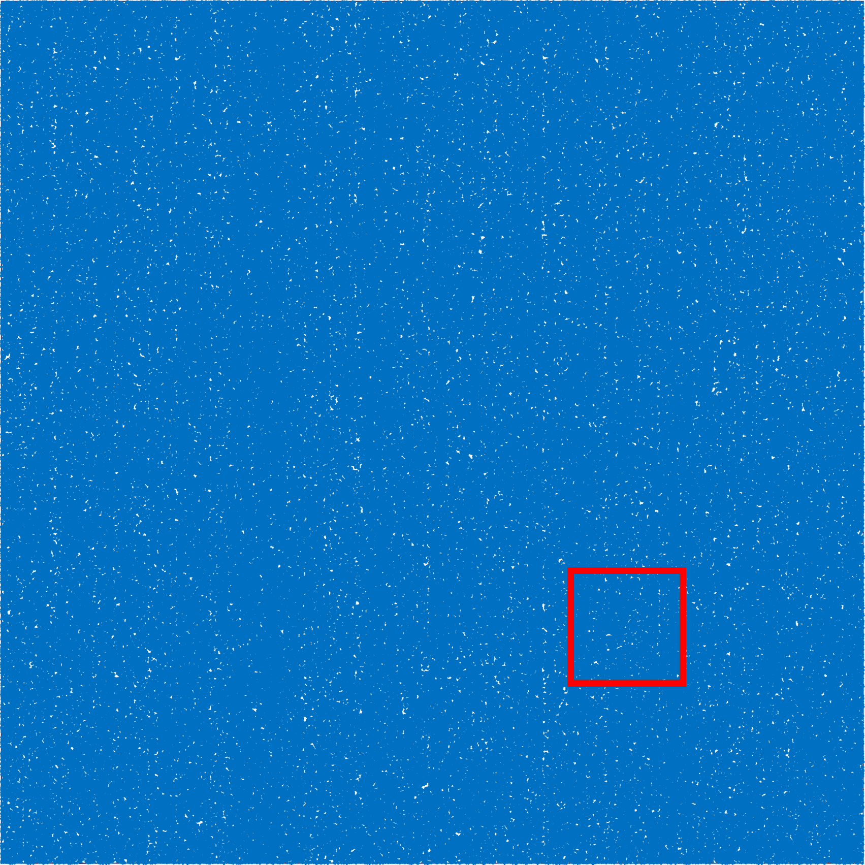
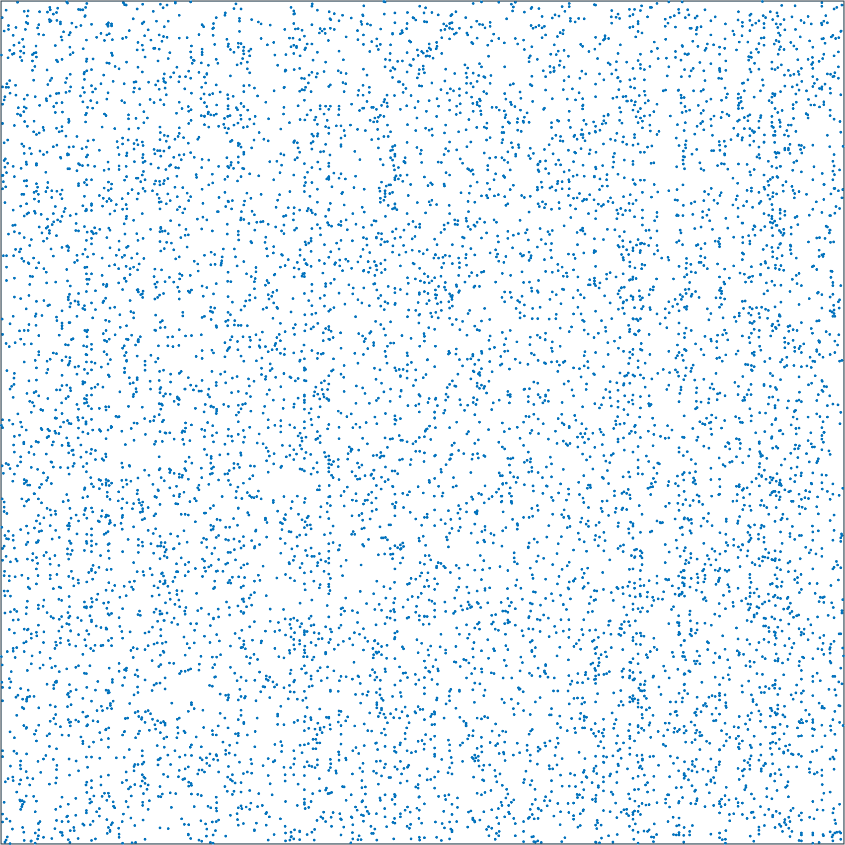
(a) scattered

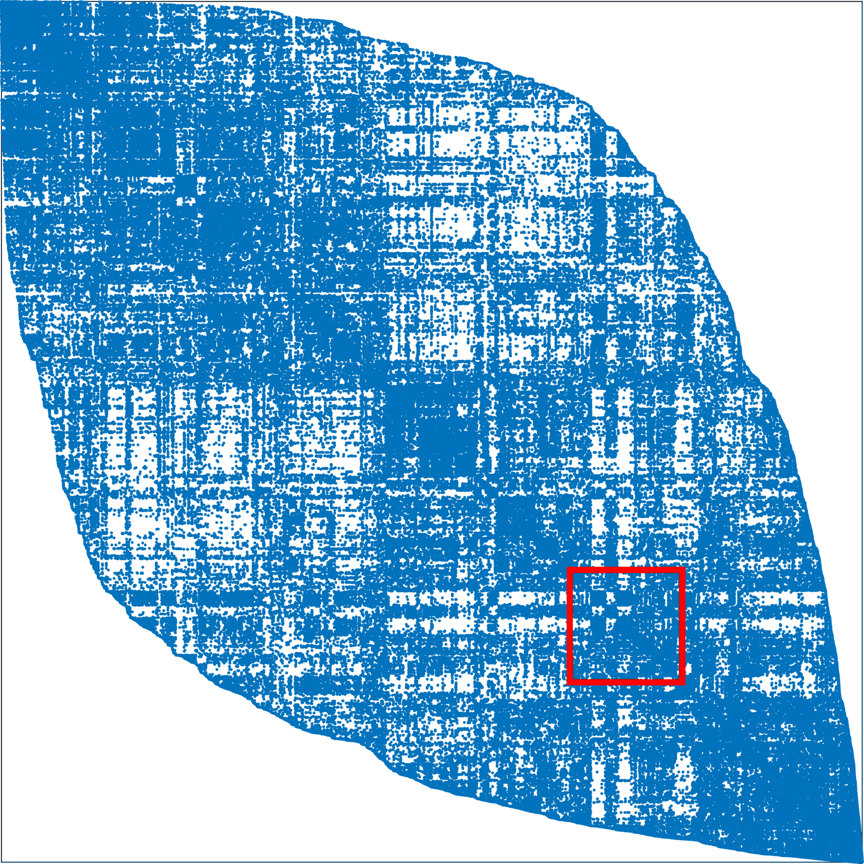
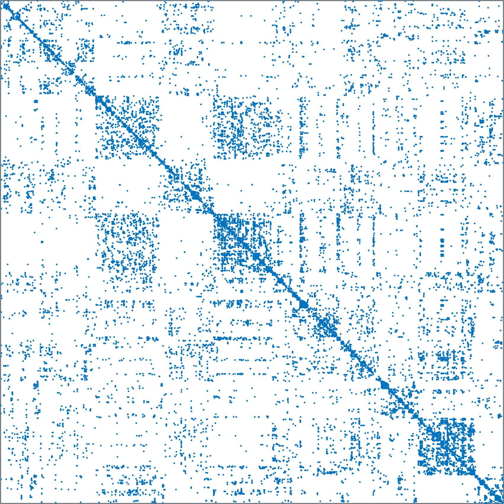
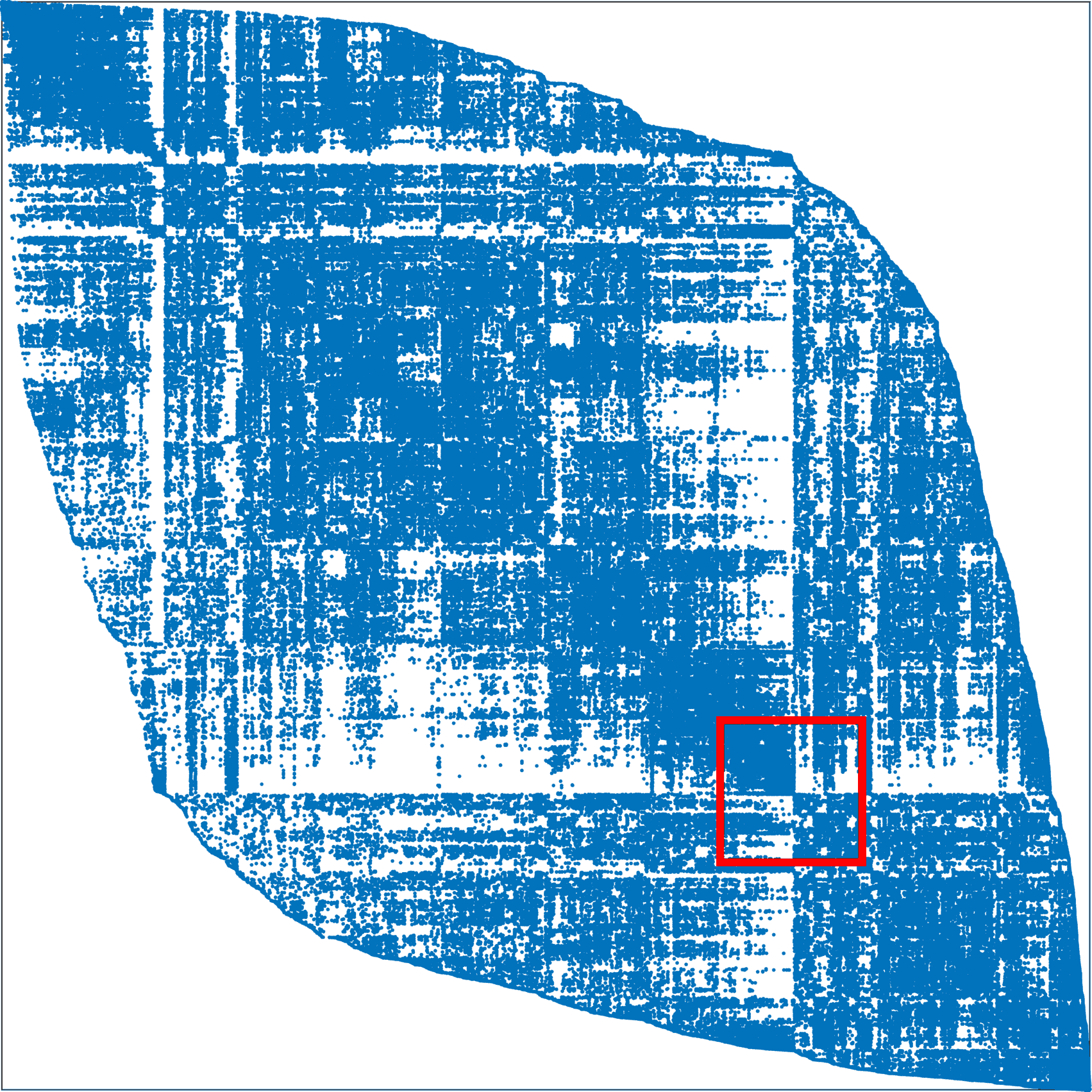
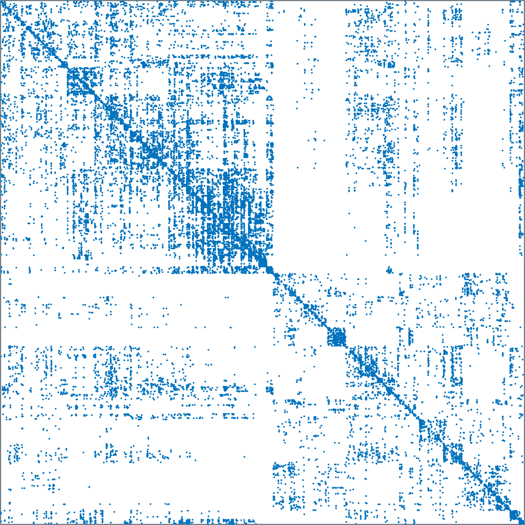
(b) rCM

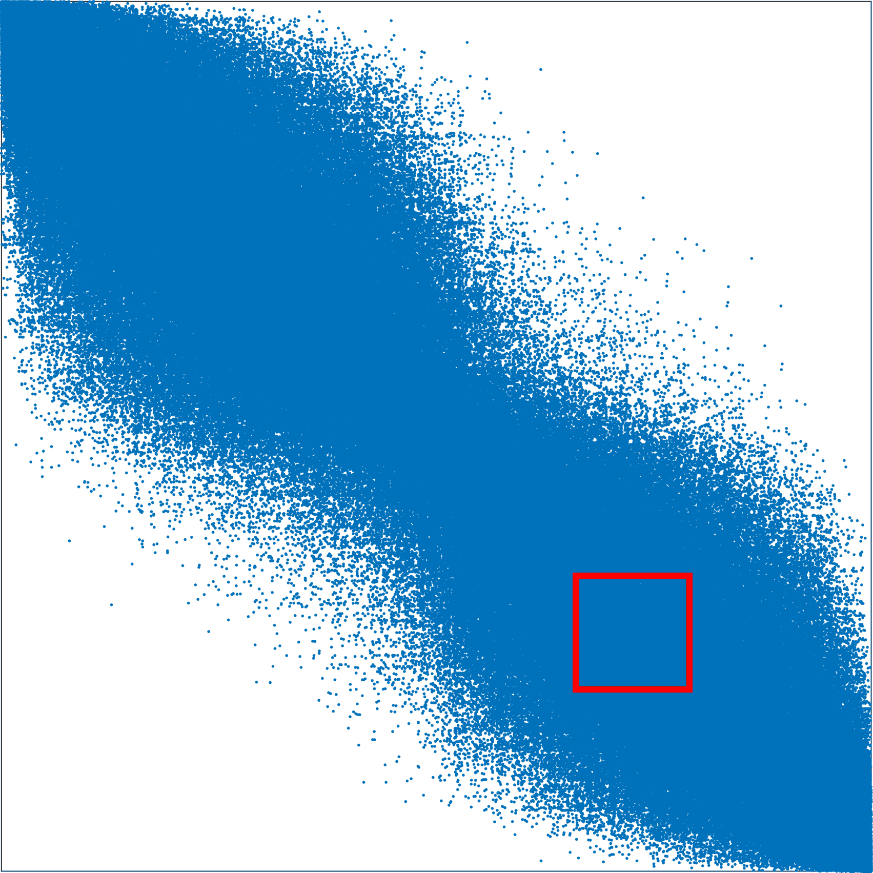
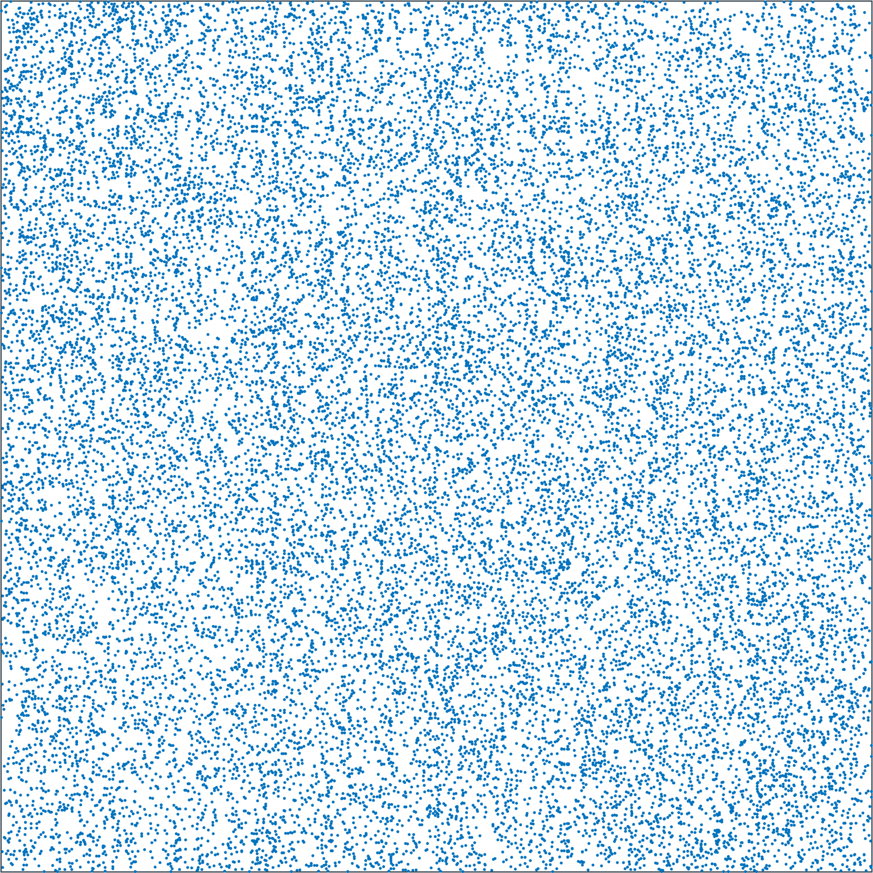
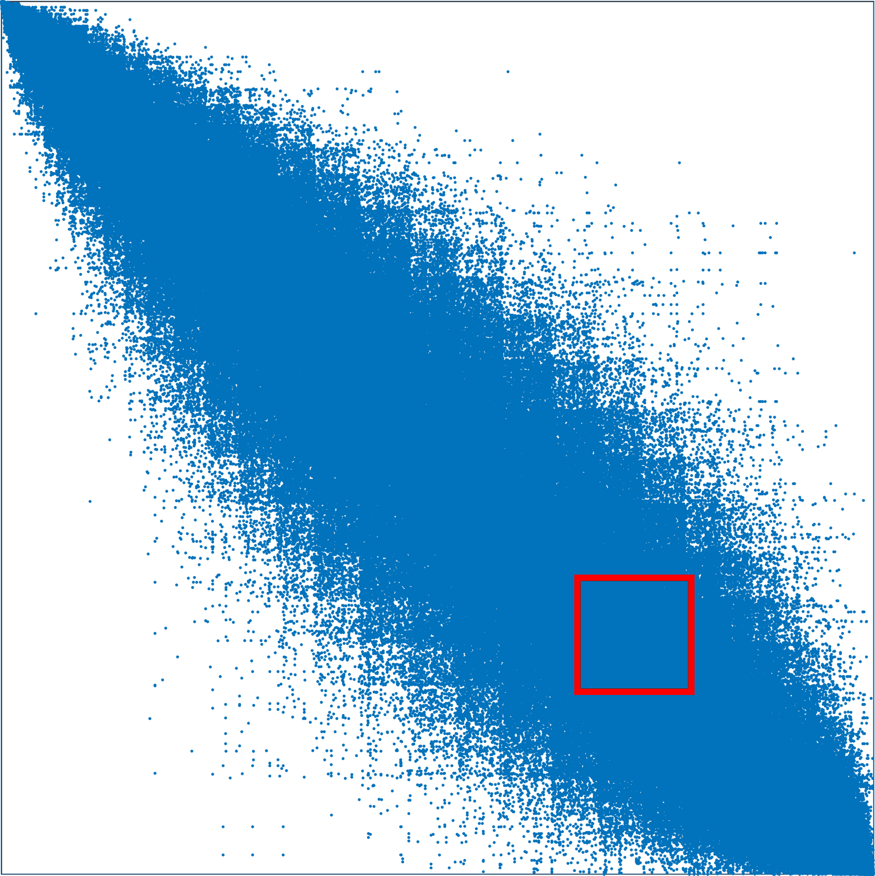
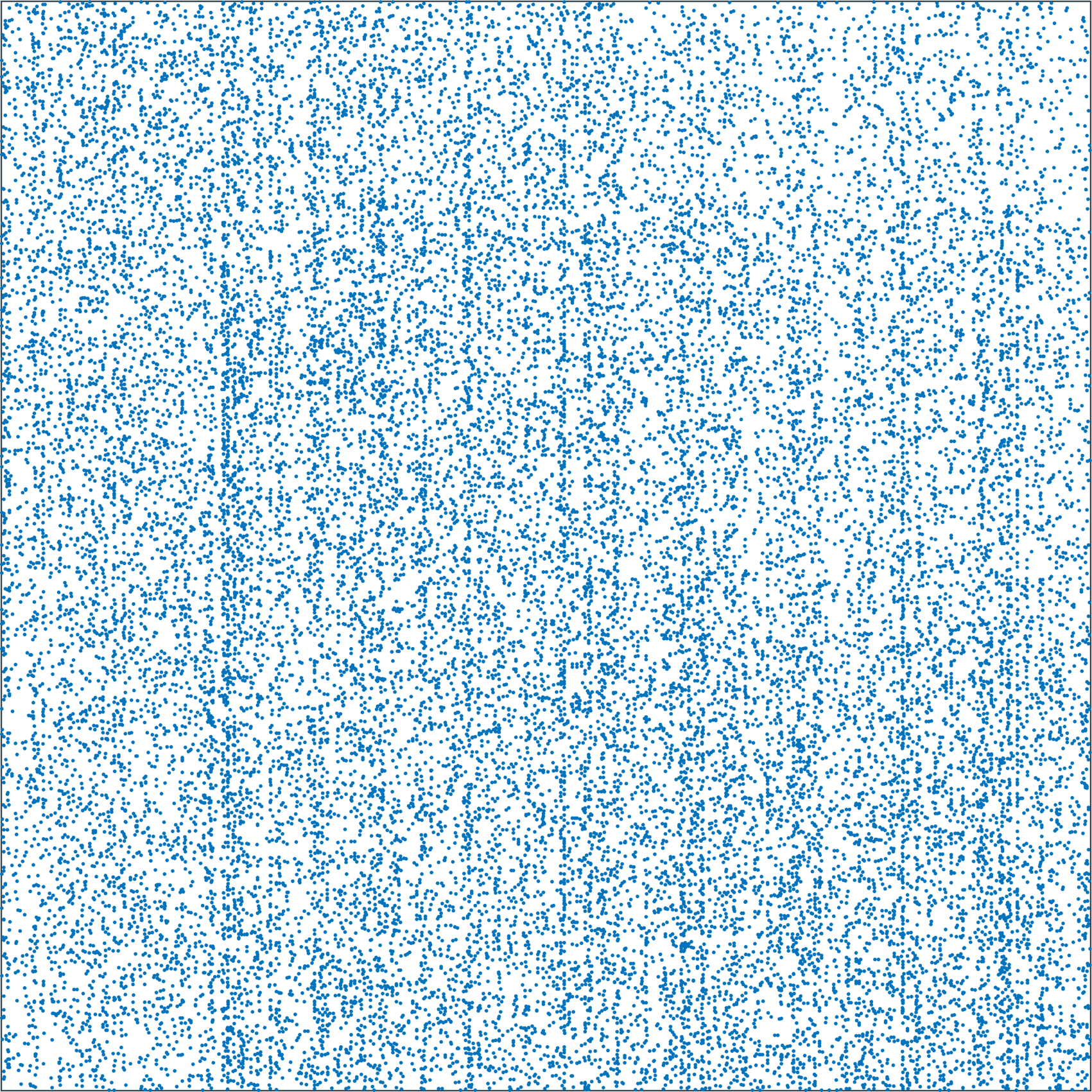
(c) 1D

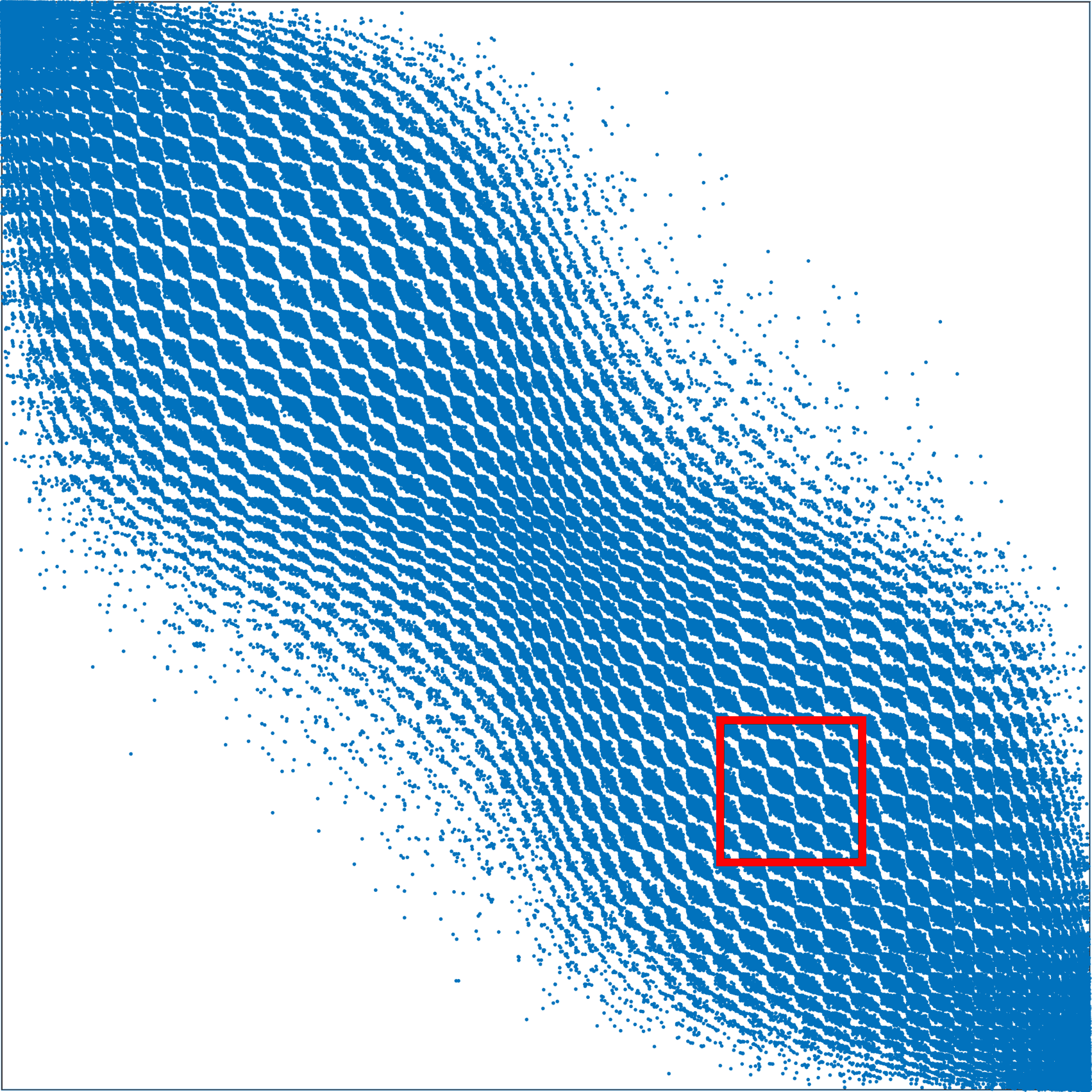
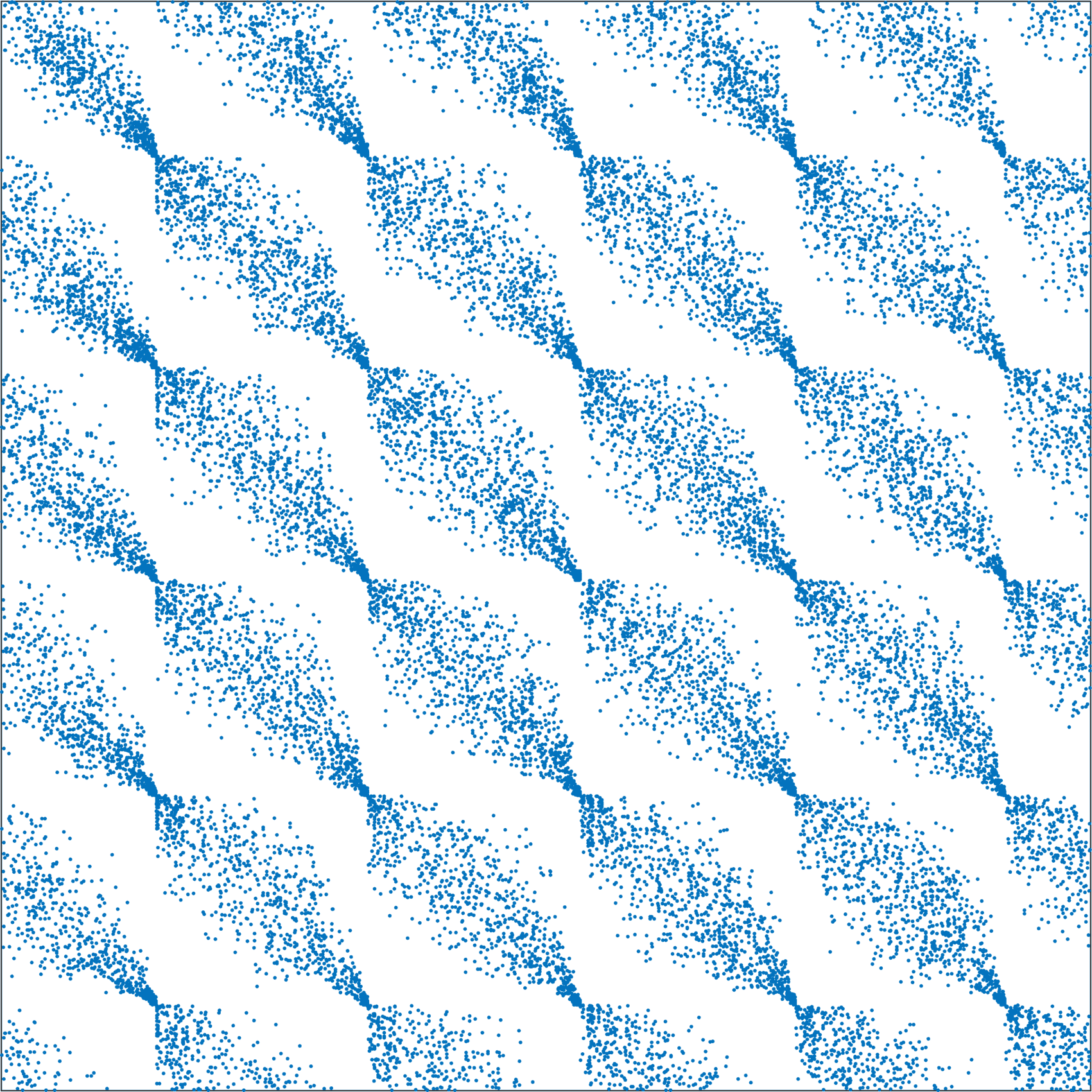
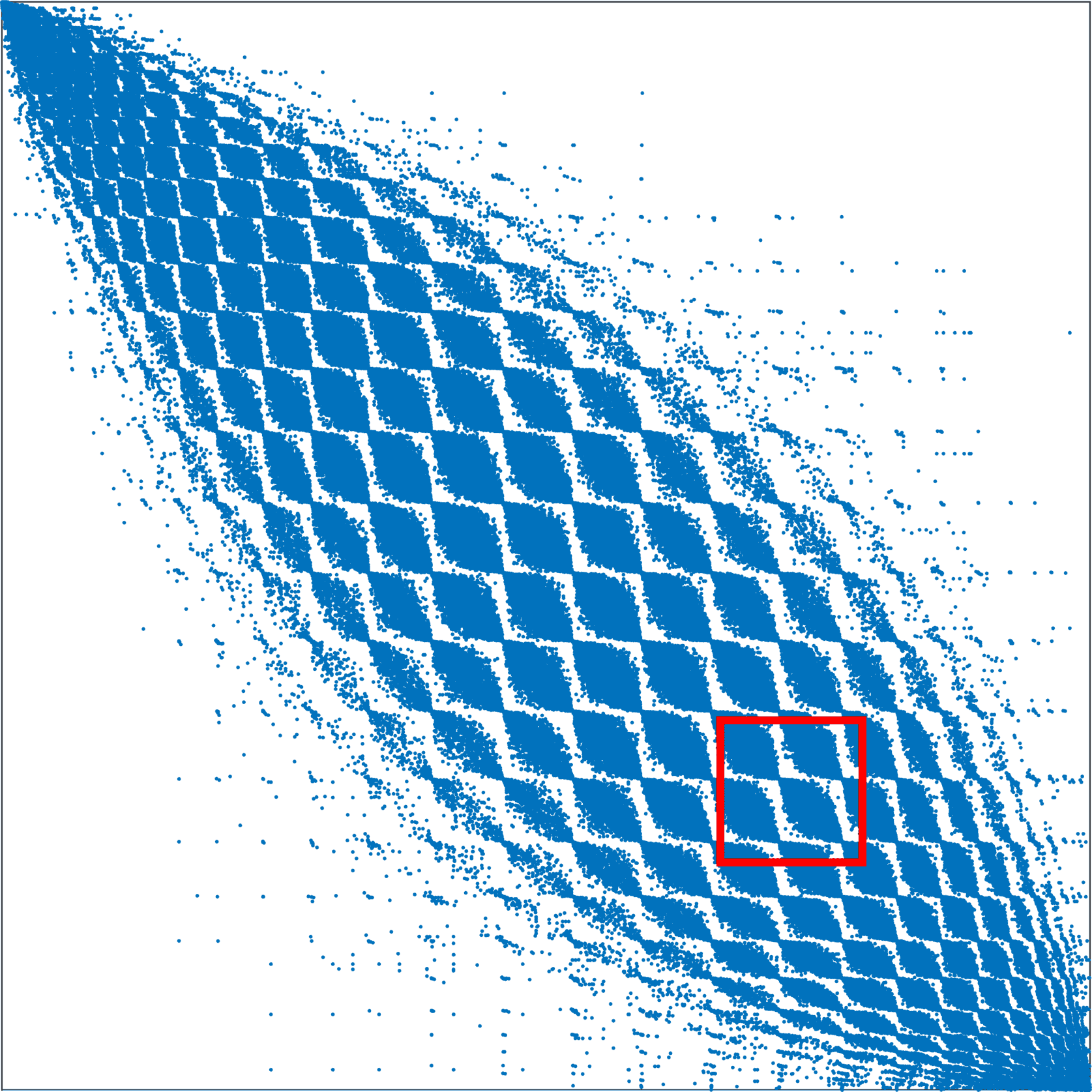
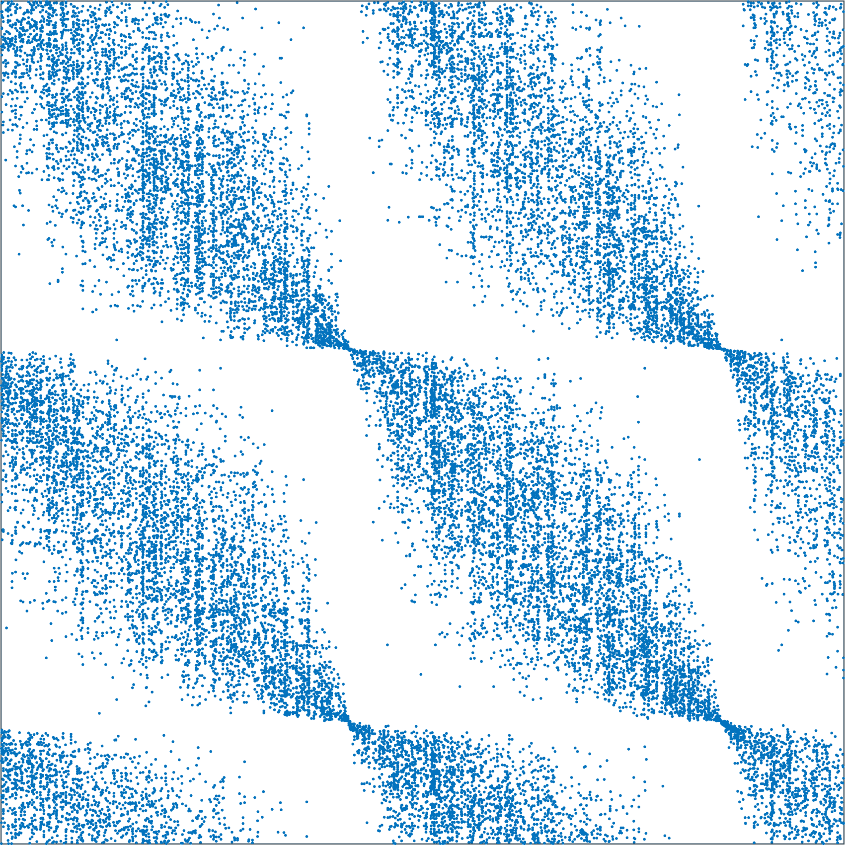
(d) 2D lexical

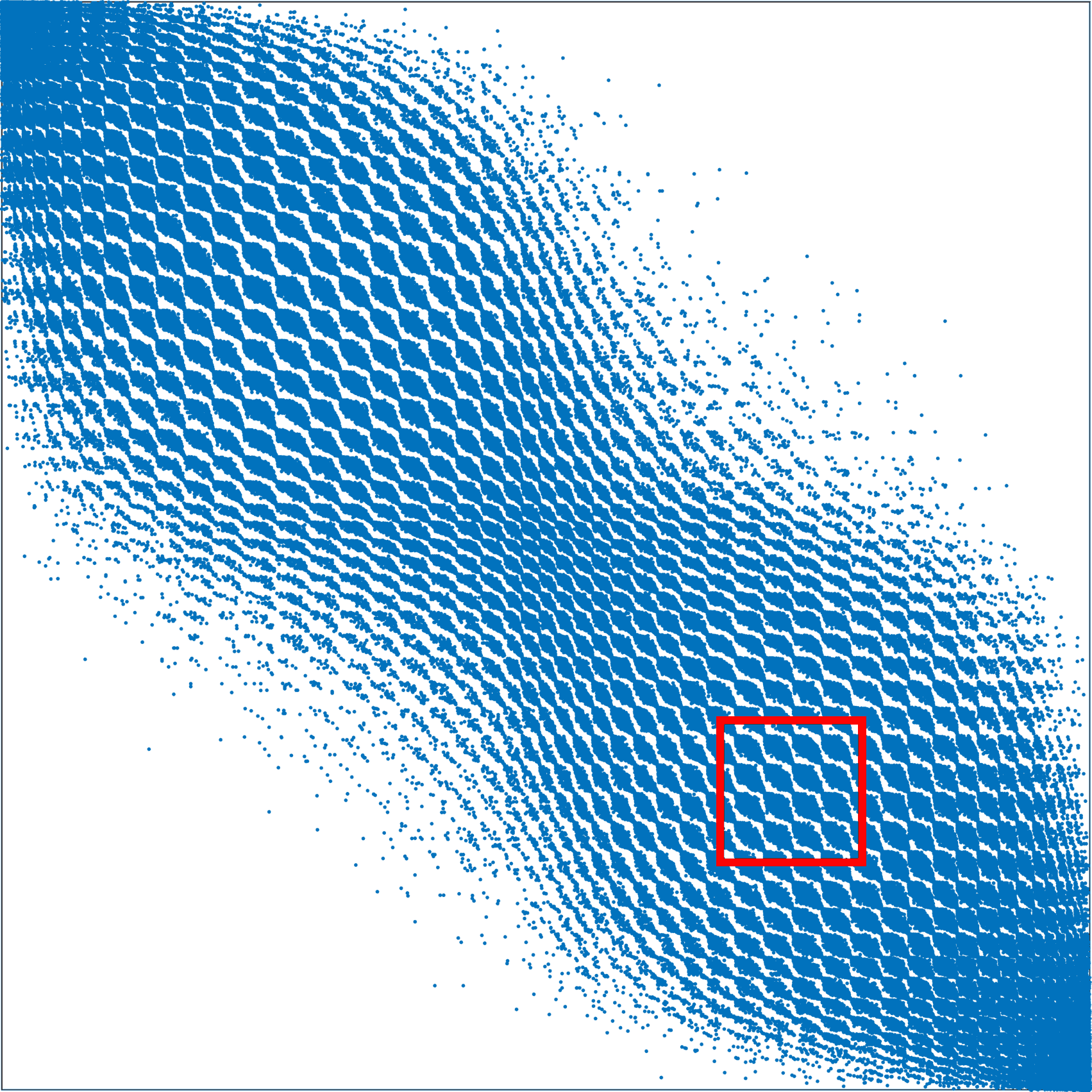
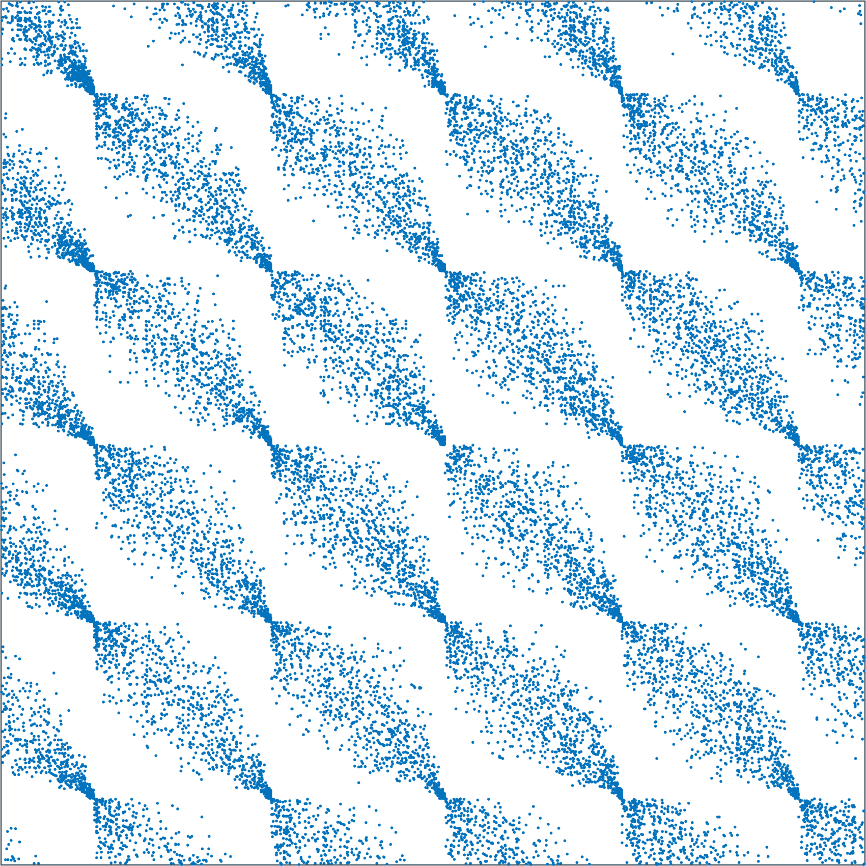
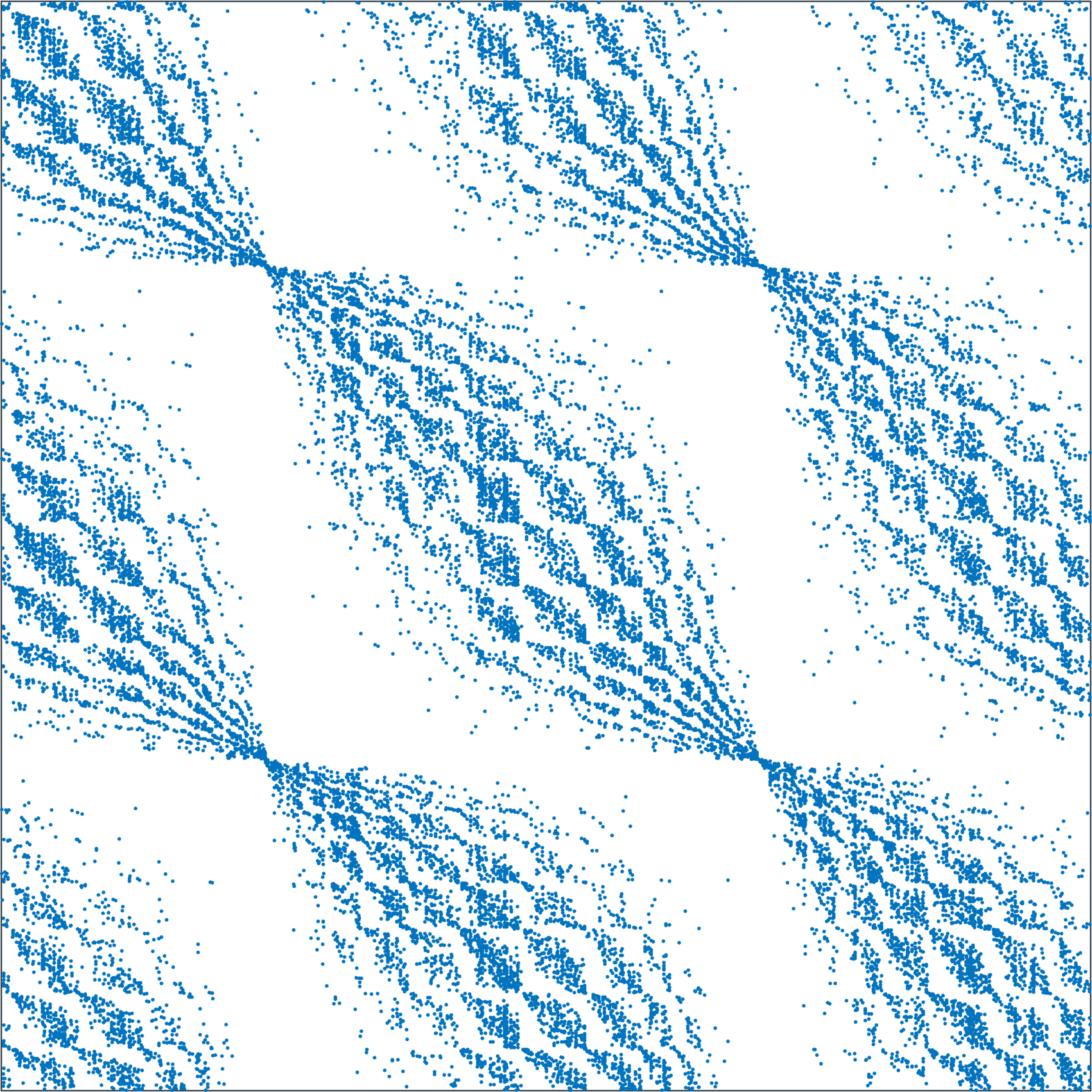
(e) 3D lexical

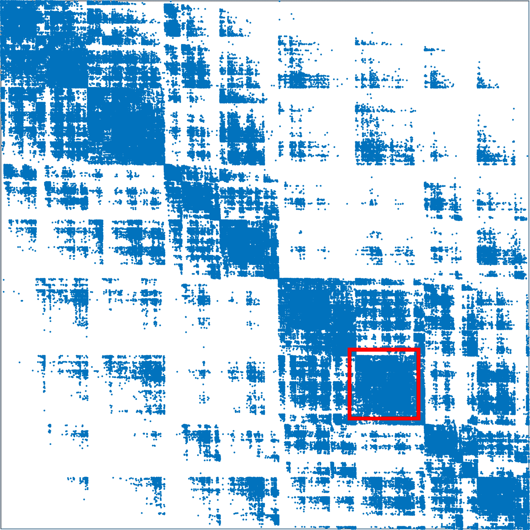
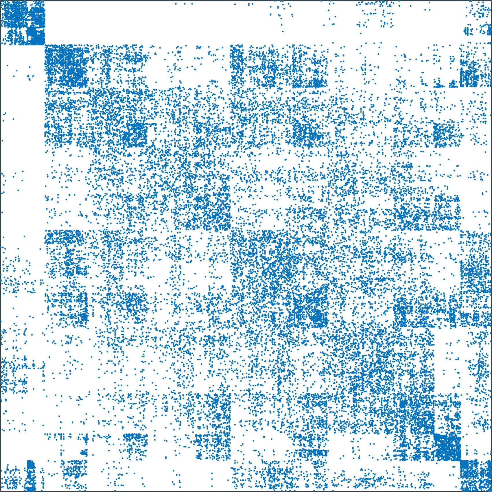
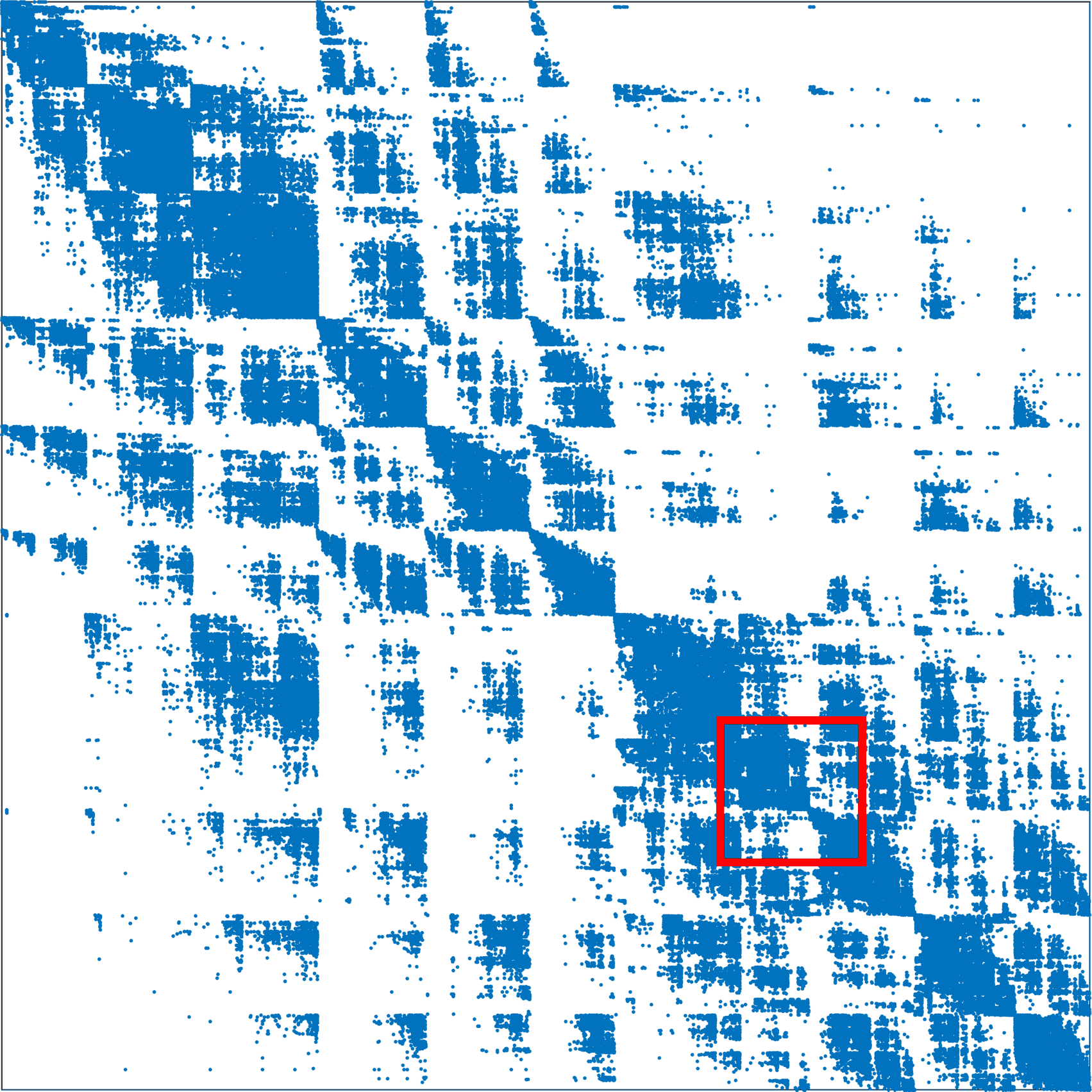
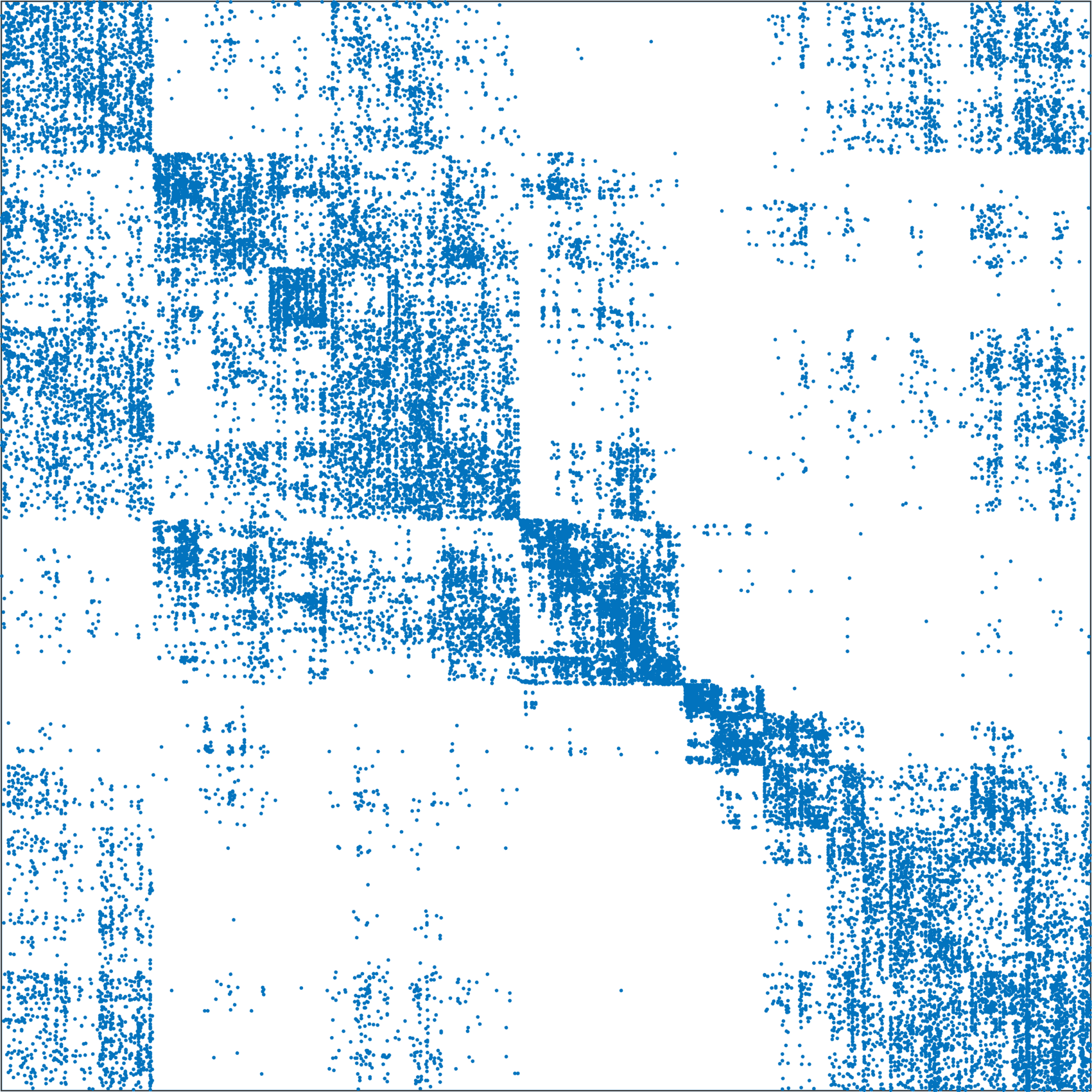
(f) 3D dual tree

Figure 2. Sparse profiles and ROI/sub-matrix details of high-dimensional interaction matrices under different orderings. These matrices capture symmetrized interactions between $2^{14}$ randomly selected points from the SIFT and GIST datasets, described in Section 4.2. rCM is the reverse Cuthill-McKee ordering (George, 1971). The 1D ordering refers to sorting the data points by the most dominant PCA component coordinates. Similarly for 2D and 3D lexical ordering, using the first 2 or 3 principal components, respectively. The 3D dual tree ordering results from our hierarchical partitioning method, described in Section 2.4.

Table 1. Kernel-based approximate patch-density estimates for the SIFT and GIST dataset interaction matrices, under different orderings, $(\boldsymbol{\mathbf{\pi}}_{\text{t}},\boldsymbol{\mathbf{\pi}}_{\text{s}})$, displayed in Fig. 2. Interacting neighborhoods comprise $k$ points (varying in order to illustrate the difference in the resulting densities). Patch-density estimates are computed with $\sigma=k/2$.

Set	$k$	Patch density estimate $\gamma\mathopen{}\mathclose{{}\left(\boldsymbol{\mathbf{A}}(\boldsymbol{\mathbf{\pi}}_{\text{t}},\boldsymbol{\mathbf{\pi}}_{\text{s}});\sigma}\right)$
		rand	rCM	1D	2D lex	3D lex	3D DT
SIFT	30	$2.3$	$14.3$	$6.1$	$12.1$	$12.1$	$\bf 20.\bf 0$
GIST	90	$71.2$	$243.6$	$286.7$	$352.1$	$361.3$	$\bf 409.\bf 6$

2.4. Matrix reordering algorithm

We describe our algorithm for attaining, via matrix reordering, a sparsity profile that is block sparse with dense blocks. The central idea to the reordering is to explore and exploit intrinsic cluster structure in the data. There are three key components to the algorithm.

Low-dimensional embedding

Often, data clusters in a high dimensional feature space can be effectively and efficiently uncovered via a low-dimensional embedding. We use a nearly isotropic low-dimensional embedding method. Specifically, the embedding space we use is spanned by the most dominant/principal feature axes that are specific to the data points. This can be done by an economic-sparse version of the singular value decomposition (SVD), namely principal component analysis (PCA). The 1D embedding by the most dominant component axis is closely related to the Laplacian spectral embedding by the Fiedler eigenvector (Fiedler, 1973). Recursive use of the Fiedler eigenvectors remains restricted to 1D geometry. We advocate multi-dimensional embedding, using more than one principal axes.

Notably, dimension reduction is used in many algorithms for high dimensional data analysis. In our case study with t-SNE, for instance, the principal feature axes are readily available. In such cases, the first step in our algorithm incurs no additional computation cost. When the feature dimension $D$ is low already, the embedding step is skipped.

For our specific purpose, a modest embedding dimension serves well in practice. We will show in particular 2D and 3D embeddings, and their advantage over 1D embedding. Formally, the embedding dimension $d<D$ can be determined according to some tolerance on the distortion in pairwise distances and the geometric neighbor relations. The tolerance can be translated into the ratio $\sum_{i=1}^{d}\sigma_{i}^{2}/\mathopen{}\mathclose{{}\left\|\boldsymbol{\mathbf{X}}}\right\|_{F}^{2}$, where $\boldsymbol{\mathbf{X}}$ is the (centered) data feature array, and $\sigma_{i}$, where $i=1,\ldots,d$ are the $d$ largest singular values of $\boldsymbol{\mathbf{X}}$. The ratio can be easily and economically obtained, without requiring the computation of all $D$ singular values.

Hierarchical partitioning

In the low-dimensional embedding (or feature) space, we partition the data points hierarchically and adaptively to systematically reveal inherent cluster structure. With 3D embedding, for example, we use an adaptive octree to locate and represent the source clusters at multiple spatial scales. Hierarchical clustering of the source data leads to a multi-level blocking among the columns of the interaction matrix. Similarly, the target tree leads to a blocking among its rows. The result is a hierarchical sparsity profile of the matrix; the profile is block-sparse with dense blocks between two consecutive layers in the hierarchy.

We will demonstrate empirically that such hierarchical profiles are better than those in lexical orderings; and that multi-level clustering is better than single-level clustering.

Multi-level data structure and interactions

In order to exploit the hierarchical matrix structure, we reorder the charge and potential vectors hierarchically in memory, per their respective clusters in source and target data. We employ a multi-level sparse storage format to place and access the interaction matrix. Finally, we make the best use of the spatial locality explored and extracted from the matrix and vector data by arranging the computation ordering accordingly, i.e., the interaction is calculated at multiple levels. Specifically, we access the nonzero matrix elements block by block; the charge and potential vectors, segment by segment. A block-segment multiplication corresponds to the interaction between a source cluster and a target cluster. In a multi-level setting, each block-segment multiplication at an intermediate level is further broken down into subblock-subsegment multiplications at the next finer level.

As with our data partitioning and placement strategy, we will demonstrate empirically that multi-level computation of interactions outperforms its single-level counterpart, in both single-core and multi-core environments.

3. Case studies

Our method is motivated and tested by two important algorithms, t-SNE (Maaten and Hinton, 2008) and mean shift (Comaniciu and Meer, 2002), which are used frequently in machine learning applications. Iterative near-neighbor interactions of large data points in multi- or high-dimensional feature spaces are important building blocks in both algorithms. In the rest of this section, we briefly describe the relevant part of each of the algorithms. Experimental results will be reported in Section 4.

3.1. Attractive interaction in t-SNE gradient

The stochastic neighbor embedding (SNE) algorithm by Hinton and Roweis (Hinton and Roweis, 2003) embeds a set $\boldsymbol{\mathbf{X}}$ of high-dimensional data into a $d$-dimensional space, where $d$ is much lower than $D$, the original feature dimensionality. The embedding is such that neighbor relationships are preserved by a stochastic approach. These relationships are cast into conditional probabilities of neighborhood governed by Gaussian kernels, and are to be preserved in the low-dimensional embedding space. In a particular SNE variant by van der Maaten and and Hinton, named t-SNE, the Student t-distribution kernel is used to govern the conditional probabilities in the lower-dimensional embedding space (Maaten and Hinton, 2008). This particular algorithm has attracted a lot of attention for its application to fascinating visualization and inspection of high-dimensional data via their 2D or 3D embedding. Its applications, however, are severely hindered by computation latency, even by the accelerated version (van der Maaten, 2014).

In t-SNE, the embedding point set $\boldsymbol{\mathbf{Y}}$ is to be placed in the $d$ dimensional space by iteratively matching the conditional probabilities of neighborhood in the embedding space to those in the original feature space. The matching objective is achieved by minimizing the Kullback-Leibler (KL) divergence between the two distributions. There are two terms in the KL gradient calculation at each iteration step, named as the attractive and repulsive forces. We focus in this study on the calculation of the attractive force, which involves near-neighbor interactions. In a fixed ordering, the sparsity profile of the near-neighbor interaction matrix remains unchanged over the iteration. The values of the nonzero elements, however, vary with iterative estimates of the embedding data $\boldsymbol{\mathbf{Y}}$; the matrix is therefore updated at each iteration step.

3.2. Iterative mean shifting

The mean shift algorithm, originally by Fukunaga and Hostetler in 1975 (Fukunaga and Hostetler, 1975), got renewed interest thanks to an influential paper by Comaniciu and Meer in 2002 (Comaniciu and Meer, 2002). It has been frequently used for non-parametric cluster analysis or mode allocation in discrete data. The algorithm locates the density maxima by iterative estimating and shifting the weighted means of the data points within a neighbor range, via a kernel function with local support. A Gaussian kernel is often used. Calculation of the shift vectors can be viewed as iterative near-neighbor interactions between the currently estimated means (targets) and the provided data points (sources), governed by the kernel. During the iteration, the sources do not change, the target means shift. As a result, the sparsity structure and the numerical values of the near-neighbor interaction matrix changes with the iteration. The data clustering on the target set needs not to be updated as frequently.

4. Experiments

We present experimental results on near-neighbor interaction performance in this section. We provide empirical comparisons among matrix orderings by our method and other existing methods. The new method is superior in sequential and parallel execution.

We provide in Table 2 the specifications of two workstations used for the experiments. One is equipped with an Intel Core i7-6700 CPU (launched Q3’15) and $32\;$GB of RAM; the other has two Intel Xeon E5540 CPUs (launched Q1’10) and $48\;$GB of RAM.

Table 2. Specifications of the CPUs used in our experiments. “Thr” indicates the number of available virtual cores due to hyper-threading.

CPU	Clock	Cores	Thr	L1	L2	L3
	(GHz)			(KB)	(KB)	(MB)
$1\times$ Core i7-6700	$3.40$	$4$	$8$	$4{\times}32$	$4{\times}256$	$8$
$2\times$ Xeon E5540	$2.53$	$2{\times}4$	$16$	$8{\times}32$	$8{\times}256$	$2{\times}8$

4.1. Micro-benchmarks

We make a few benchmarks of near-neighbor interactions on the testbed machines with synthetic data to establish machine-specific references for performance assessment. We use the Intel high-performance MKL_CSC_MV implementation of the BLAS SpMV for the benchmarks.

The making of the benchmarks is as follows. For a fixed matrix size with a fixed number of nonzeros, we use the banded matrix, which corresponds to 1D interaction, to establish the best performance obtainable on the particular machines. To establish the base case, we use a matrix with the nonzero elements randomly scattered. In both cases, the matrix elements are in compressed storage format and referenced via indirect addresses. The benchmarks with the synthetic data are to be used in Section 4.3 as a reference for assessing the performance of near-neighbor interactions with real-world datasets described in the next section.

4.2. Datasets

The data sets used in the experiments are drawn from the following two big datasets, which are publicly available:

SIFT:

128-dimensional SIFT feature vectors (Lowe, 2004) extracted from images of the INRIA Holidays dataset (Jégou et al., 2008).

GIST:

960-dimensional GIST feature vectors (Oliva and Torralba, 2001) extracted from images of the tiny image set (Torralba et al., 2008).

Speed-up over sequential scattered

Speed-up over sequential scattered

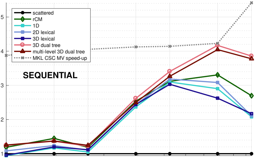
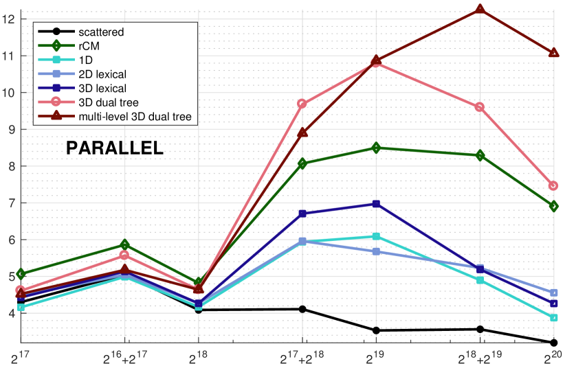
Number of data points

(a) SIFT dataset; Core i7-6700 workstation

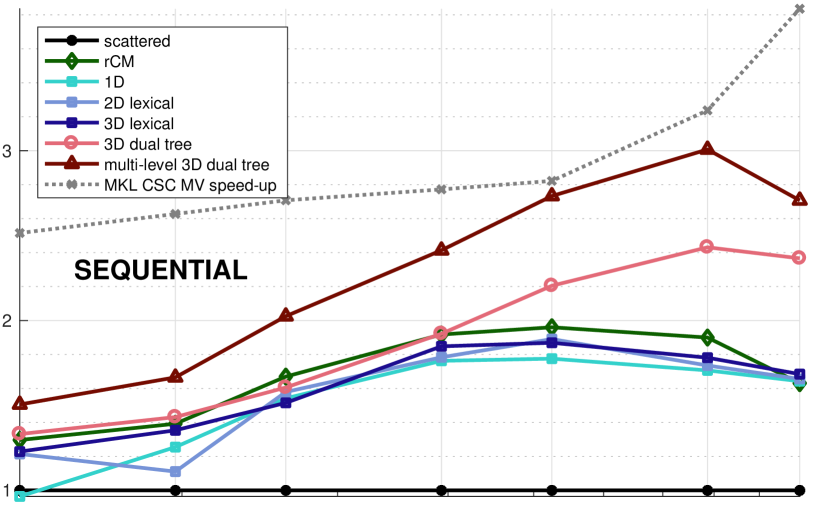
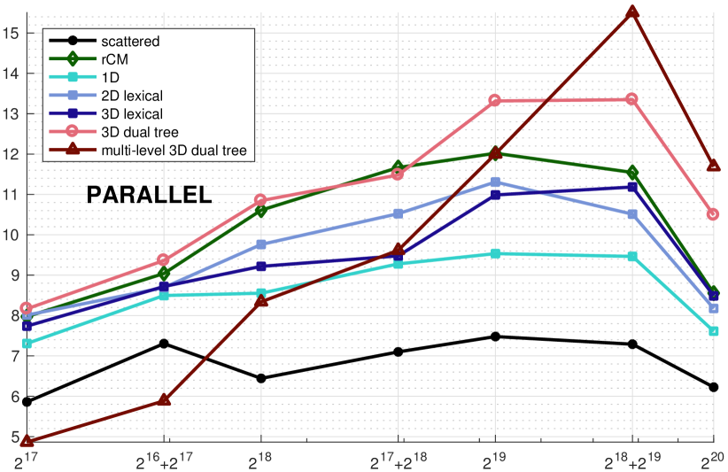
Number of data points

(b) GIST dataset; Xeon E5540 workstation

Figure 3. Comparison in performance by different ordering schemes used for attractive force calculation in t-SNE. The top plots show the comparison in sequential execution; the bottom, in parallel. The plots to the left are associated with the SIFT data on the Core i7-6700 workstation; to the right, with the GIST data on the Xeon E5540 workstation. The solid black line in each case corresponds to the case with randomly scattered ordering. The sequential execution time is used as the reference time, for comparisons in sequential execution as well as parallel execution. More details are in the text.

4.3. Performance

We provide in Fig. 3 the comparison in performance among several ordering schemes used for the attractive force calculation in t-SNE. The comparisons are made on both data sets, in sequential execution as well as in parallel execution. The reference time for the comparisons is the sequential execution time with the scattered ordering.

The following particular orderings are used in the comparisons: 1 “scattered,” by random permutation of the interacting points placement; 2 “rCM,” the reverse Cuthill-McKee ordering; 3 “1D,” where the data points (rows and columns) are sorted by the most dominant PCA component coordinates; 4 “2D lexical” and 5 “3D lexical,” by lexicographic sorting of the first 2 or 3 principal components, respectively; and 6 “3D dual tree,” by our matrix reordering algorithm, described in Section 2.4. The sparse matrix profiles associated with each of orderings are shown in Fig. 2.

The dotted gray lines in the top plots show the time ratio of the execution time of MKL_CSC_MV as per the micro-benchmarks discussed in Section 4.1 (speed-up of banded over scattered matrix operations). The number of nonzero elements per row is constant and matches the sparsity of the SIFT and GIST near-neighbor interaction matrices on the corresponding workstation experiments. These time ratios are used as a reference for the maximum expected improvement to be gained by matrix reordering.

The speed-up in parallel execution by our new method reaches $12{\times}$ on the Core i7 and more than $15{\times}$ on the Xeon E5540. Compared to the popular rCM ordering, the multi-level 3D dual tree ordering is about 40% faster for larger problem sizes, when the data size exceeds the size of the L3 cache. On both workstations and datasets, the sequential execution improvement with our reordering approaches the MKL_CSC_MV time ratio for certain sizes.

We underline the following observations. By multi-dimensional embedding, our method explores more potential in data clustering; this leads to better matrix sparsity profiles, improved data locality, reduced memory latency, and hence fast execution time. The performance with hierarchical ordering outperforms that with the lexical orderings in the same embedding space. This shows the importance of integrating multi-dimensional embedding with hierarchical clustering. The latter is followed by multi-level data placement, and multi-level interactions. The comparisons are consistent with what we expected from the respective sparity profiles in Fig. 2.

5. Related work & discussion

Improving data locality in sparse matrix computation by reordering the matrix at the algorithm level has a long and rich history. It becomes more important with modern computers and computation applications. The CM ordering by Cuthiil and McKee was reported in 1969 (Cuthill and McKee, 1969); the reverse CM (rCM) ordering appeared two years later (George, 1971). Davis et al. provided in 2016 a survey of fill-reducing orderings in direct methods for sparse linear systems (Davis et al., 2016).

Our method assumes that the sparse matrix is defined over coordinated data and represents near-neighbor interactions. In particular, the feature vectors serve as coordinate vectors. Exploiting coordinate attributes in the data was discussed in (Mellor-Crummey et al., 2001) and the references therein. The dimension of the coordinate space was low. In modern data and image analysis, the feature dimension is typically much higher. High dimensionality exposes the limitation of previous sparsity profiles. For example, the size of the bandwidth envelope is essentially a 1D measure, relying on a 1D embedding of multi-dimensional data. In particular, 1D Laplacian spectral embedding by the Fiedler vector (Fiedler, 1973) is frequently used in previous work to reduce the size of bandwidth envelope (Barnard et al., 1995). We advocate multi-dimensional embedding, instead.

Multi-dimensional embedding serves two objectives simultaneously: near-isometric dimension reduction, and multi-level clustering in the lower-dimensional space. The final goal is to attain a desirable matrix sparsity profile. Our method does not invoke the formation of a Laplacian graph when it is not readily available. The recursive bisection method by the Fiedler vectors of partitioned subgraphs may be viewed as multi-level clustering. It is, however, limited to 1D embedding geometry. Our multi-level partition is in a multi-dimensional space, without entailing computation of recursive Fiedler vectors.

Our assumption and method are directly applicable to a broad class of data and operations for data analysis. This class includes mesh data in various scientific simulations; it includes graph or network data with attributes on the graph nodes and/or edges. Investigation of graph-related sparse compression and computation is reported in Chapter 8 of Shun’s dissertation in 2017 (Shun, 2017).

Our multi-level compressed sparse storage format has a connection to the Compressed Sparse Block (CSB) scheme by Buluç et al. (Buluç et al., 2009). CSB makes, stores, and accesses uniform blocks of a preset size, assuming no knowledge of data coordinates and cluster structure. By such blocking, the distance between successive accesses to the entries in the same matrix block is bounded constant from above, away from the growing data size. Our scheme reduces to CSB when the hierarchy is flat, i.e., with only a single level of blocks, except that the blocks at the bottom level are more or less uniform in the number of nonzeros, but not necessarily uniform in block area. At a higher level in our compression hierarchy, the blocks are pointers for indirect references to hierarchically placed data.

The temporal ordering, or partial ordering, in computational execution must be compatible with the spatial ordering, relationship, and placement of data. Although well noted in previous work, this spatio-temporal compatibility warrants special attention and effort in algorithm development and implementation.

In summary: 1 Our method for ordering a sparse matrix by multi-scale clustering of high-dimensional data is based on a novel concept and model of desirable sparsity profiles. Our block-sparse with dense blocks model and the related patch density measure capture and characterize the essential properties in an interaction matrix that are conducive to better space and time locality. The model and measure unify several previous sparsity profile models in the sense that our model favors the same profile favored by another one when the data meet the condition(s) by the latter. 2 Our method is empirically shown to be superior to previous, popular methods in sequential computation on a single core, and even better in parallel computation on multiple cores.

- (1)
- Barnard et al. (1995) Stephen T. Barnard, Alex Pothen, and Horst Simon. 1995. A spectral algorithm for envelope reduction of sparse matrices. Numerical Linear Algebra with Applications 2, 4 (1995), 317–334.
- Buluç et al. (2009) Aydin Buluç, Jeremy T. Fineman, Matteo Frigo, John R. Gilbert, and Charles E. Leiserson. 2009. Parallel sparse matrix-vector and matrix-transpose-vector multiplication using compressed sparse blocks. In Proceedings of the 21st Annual Symposium on Parallelism in Algorithms and Architectures. 233–244.
- Comaniciu and Meer (2002) Dorin Comaniciu and Peter Meer. 2002. Mean shift: a robust approach toward feature space analysis. IEEE Transactions on Pattern Analysis and Machine Intelligence 24, 5 (2002), 603–619.
- Cuthill and McKee (1969) Elizabeth Cuthill and James McKee. 1969. Reducing the bandwidth of sparse symmetric matrices. In ACM Proceedings of the 24th National Conference. 157–172.
- Davis et al. (2016) Timothy A. Davis, Sivasankaran Rajamanickam, and Wissam M. Sid-Lakhdar. 2016. A survey of direct methods for sparse linear systems. Acta Numerica 25 (2016), 383–566.
- Fiedler (1973) Miroslav Fiedler. 1973. Algebraic connectivity of graphs. Czechoslovak Mathematical Journal 23, 2 (1973), 298–305.
- Fukunaga and Hostetler (1975) Keinosuke Fukunaga and Larry D. Hostetler. 1975. The estimation of the gradient of a density function, with applications in pattern recognition. IEEE Transactions on Information Theory 21, 1 (Jan. 1975), 32–40.
- George et al. (1986) Alan George, Michael T. Heath, Joseph Liu, and Esmond Ng. 1986. Solution of sparse positive definite systems on a shared-memory multiprocessor. International Journal of Parallel Programming 15, 4 (1986), 309–325.
- George (1971) Alan J. George. 1971. Computer implementation of the finite element method. Ph.D. Dissertation. Department of Computer Science, Stanford University, Palo Alto, CA, USA.
- Hinton and Roweis (2003) Geoffrey Hinton and Sam Roweis. 2003. Stochastic Neighbor Embedding. In Advances in Neural Information Processing Systems 15.
- Jégou et al. (2008) Hérve Jégou, Matthijs Douze, and Cordelia Schmid. 2008. Hamming embedding and weak geometric consistency for large scale image search. In Proceedings of the 10th European Conference on Computer Vision: Part I (ECCV ’08). Springer-Verlag, Berlin, Heidelberg, 304–317.
- Lowe (2004) David G. Lowe. 2004. Distinctive image features from scale-invariant keypoints. International Journal of Computer Vision 60, 2 (2004), 91–110.
- Maaten and Hinton (2008) Laurens van der Maaten and Geoffrey Hinton. 2008. Visualizing data using t-SNE. Journal of Machine Learning Research 9, Nov (2008), 2579–2605.
- Mellor-Crummey et al. (2001) John Mellor-Crummey, David Whalley, and Ken Kennedy. 2001. Improving memory hierarchy performance for irregular applications using data and computation reorderings. Int. J. Parallel Program. 29, 3 (2001), 217–247.
- Oliva and Torralba (2001) Aude Oliva and Antonio Torralba. 2001. Modeling the shape of the scene: A holistic representation of the spatial envelope. International journal of computer vision 42, 3 (2001), 145–175.
- Rixner et al. (2000) Scott Rixner, William J. Dally, Ujval J. Kapasi, Peter Mattson, and John D. Owens. 2000. Memory access scheduling. ACM SIGARCH Computer Architecture News 28, 2 (2000), 128–138.
- Shun (2017) Julian Shun. 2017. Shared-memory parallelism can be simple, fast, and scalable. Ph.D. Dissertation. School of Computer Science, Carnegie Mellon University, Pittsburgh, PA, USA. CMU-CS-15-108.
- Torralba et al. (2008) Antonio Torralba, Rob Fergus, and William T. Freeman. 2008. 80 million tiny images: a large data set for nonparametric object and scene recognition. IEEE Transactions on Pattern Analysis and Machine Intelligence 30, 11 (2008), 1958–1970.
- van der Maaten (2014) Laurens van der Maaten. 2014. Accelerating t-SNE using tree-based algorithms. J. Mach. Learn. Res. 15, 1 (2014), 3221–3245.