Lens covariance effects on likelihood analyses of CMB power spectra

Abstract

Non-Gaussian correlations induced in CMB power spectra by gravitational lensing must be included in likelihood analyses for future CMB experiments. We present a simple but accurate likelihood model which includes these correlations and use it for Markov Chain Monte Carlo parameter estimation from simulated lensed CMB maps in the context of $\Lambda$CDM and extensions which include the sum of neutrino masses or the dark energy equation of state $w$. If lensing-induced covariance is not taken into account for a CMB-S4 type experiment, the errors for one combination of parameters in each case would be underestimated by more then a factor of two and lower limits on $w$ could be misestimated substantially. The frequency of falsely ruling out the true model or finding tension with other data sets would also substantially increase. Our analysis also enables a separation of lens and unlensed information from CMB power spectra, which provides for consistency tests of the model and, if combined with other such measurements, a nearly lens-sample-variance free test for systematics and new physics in the unlensed spectrum. This parameterization also leads to a simple effective likelihood that can be used to assist model building in case consistency tests of $\Lambda$CDM fail.

I Introduction

Measurements of the cosmic microwave background (CMB) have been instrumental in our understanding of the composition and evolution of the Universe (see e.g. Ade et al. (2016a)). Starting with the initial detection through cross correlation of the quadratic reconstruction of the lensing potential Hu (2001) with galaxy surveys Smith et al. (2007), gravitational lensing of the CMB by the large scale structure of the Universe (see Lewis and Challinor (2006) for a review) has emerged as a new source of cosmological information Hirata et al. (2008); Hanson et al. (2013); Das et al. (2011); Keisler et al. (2011); Ade et al. (2014); Keisler et al. (2015); Ade et al. (2016b, c); Sherwin et al. (2017). For currently operating and future CMB experiments Benson et al. (2014); Henderson et al. (2016); Wu et al. (2016); Abazajian et al. (2016), gravitational lensing will be instrumental in breaking parameter degeneracies affecting low redshift physics, such as sum of the neutrino masses and properties of the dark energy.

On the other hand, lensing also acts as a source of lens-sample-variance noise for the detection of inflationary gravitational waves and light relic particles from CMB power spectra (see e.g. Abazajian et al. (2016)). Lens sample variance can be removed by reconstructing the lensing potential assuming that the power spectra and higher point moments are lensed by the same potential. Recently, Ref. Motloch et al. (2017) proposed a consistency test between the two that can be used to protect against systematic errors and incorrect assumptions on either side.

The covariance between CMB observables induced by lensing also complicates their analysis. This covariance was first studied between the lensed temperature and polarization power spectra Smith et al. (2006); Benoit-Levy et al. (2012), yet all analyses of CMB experiments to date have omitted it in the likelihood function (e.g. Ade et al. (2016a)). Once polarization measurements approach the sample variance limit, this covariance must be included in the analysis Benoit-Levy et al. (2012) as well as the correlation between power spectra and the reconstructed lensing potential Green et al. (2016); Peloton et al. (2016); Motloch et al. (2017).

Most previous studies have employed Fisher forecasts to estimate lens-covariance effects on parameter constraints rather than a direct likelihood exploration, with the exception of Peloton et al. (2016) who briefly investigate their impact on neutrino mass constraints in $\Lambda$CDM. The main goal of this work is filling this gap with a more comprehensive study of an analysis pipeline from simulated lensed CMB maps to parameter posterior probabilities, including the principal component parameterization of the lensing potential introduced in Ref. Motloch et al. (2017).

This paper is organized as follows. In § II we present our model for the likelihood function of full-sky CMB power spectra data which accounts for lensing-induced covariance between multipole moments. We briefly review the analytical model for the lensing-induced covariance upon which it is based Benoit-Levy et al. (2012) and define the fiducial cosmology and experimental configuration investigated in this work. Then in § III we look at effects the non-Gaussian covariance has on cosmological parameter constraints and point out that neglecting this covariance could have a possibly serious impact on concordance studies. In § IV we introduce a principal component parameterization of lensed CMB power spectra, describe results of our MCMC analyses of properties of these parameters and use them to explain the effects of lensing-induced covariance on cosmological parameters. In the same section we then detail how measurements of these effective parameters can be used to form consistency tests for the data and assist model building.

In the Appendices we give more details on how we modify code Lenspix which simulates lensed CMB data to achieve high accuracy (Appendix A), how effects of the non-Gaussian covariance change for an experiment which does not measure information on the largest scales (Appendix B) and how we determined necessary number of lensing principal components (Appendix C).

II Analysis details

In this section we first describe our fiducial cosmology and experimental configuration. Then we comment on analytic model used for the covariance of lensed CMB power spectra, details of our CMB simulations and Markov Chain Monte Carlo analysis and in a separate section we describe our model for the data likelihood.

II.1 Fiducial cosmology and experimental setup

In this work we investigate a simplified experimental setup of a full sky experiment with specifications inspired by CMB Stage 4 Abazajian et al. (2016). Throughout the paper we use capital letters $X,Y,W,Z$ to represent either CMB temperature or polarization field, i.e. an element from $\{T,E,B\}$. In a given cosmological model, we also abbreviate the set of all cosmological parameters as $\theta_{A}$. We consider the information on $\theta_{A}$ provided by the CMB power spectra $C_{\ell}^{XY}$.

For the fiducial cosmology we take a flat 6 parameter $\Lambda$CDM model with minimal neutrino mass. For the $\Lambda$CDM parameters we take $\omega_{b}=\Omega_{b}h^{2}$, the physical baryon density; $\omega_{c}=\Omega_{c}h^{2}$, the physical cold dark matter density; $n_{s}$, the tilt of the scalar power spectrum; $A_{s}$, its amplitude; and $\tau$, the optical depth to recombination. We choose $\theta_{*}$, the angular scale of the sound horizon at recombination, as opposed to the Hubble constant $h$, as the sixth independent parameter. We also assume that tensor modes are negligible so that there is no unlensed $B$ mode. Values of the cosmological parameters for the fiducial model used in this work are summarized in Table 1.

Table 1: Fiducial parameters used in the analysis

Parameter	Fiducial value
$h$	0.675
$\Omega_{c}h^{2}$	0.1197
$\Omega_{b}h^{2}$	0.0222
$n_{s}$	0.9655
$A_{s}$	$2.196\times 10^{-9}$
$\tau$	0.06
$\sum m_{\nu}$	60 meV

For noise in temperature and polarizations, we assume a noise spectra Knox (1995)

$$N_{\ell}^{XY}=\Delta_{XY}^{2}e^{\ell(\ell+1){\theta_{\mathrm{FWHM}}^{2}}/{8{\ln}2}},$$ (1)

where $\Delta_{XY}$ is the instrumental noise (in $\mu$K-radian) and $\theta_{\mathrm{FWHM}}$ is the beam size (in radians). We consider a $1^{\prime}$ beam, $\Delta_{TT}=1\,\mu$K^′, $\Delta_{EE}=\Delta_{BB}=1.4\,\mu$K^′, and $\Delta_{TE}=\Delta_{TB}=\Delta_{EB}=0$ and use measurements in the multipole range $\ell=2-3000$.

II.2 Data covariance

Because all CMB temperature and polarization anisotropies are lensed by the same realization of the lensing potential, the lensed CMB power spectra data are correlated across multipoles. The ensuing covariance can be well described by a simple analytical model which has been tested on simulations Benoit-Levy et al. (2012). Recently, this model has been extended to capture correlations of the lensed CMB power spectra with the lensing potential $C^{\hat{\phi}\hat{\phi}}_{\ell}$ reconstructed by a quadratic estimator Green et al. (2016); Peloton et al. (2016); Motloch et al. (2017). Here we describe salient features of this model, more in-depth discussion and graphical representation of the resulting covariances can be found in the references.

In this model the correlation matrix is split into “Gaussian part” $\mathcal{G}$ that is diagonal in multipole space and $\mathcal{N}$ which describes non-Gaussian correlations between multipoles,

$$\mathrm{Cov}^{XY,WZ}_{\ell\ell^{\prime}}=\mathcal{G}^{XY,WZ}_{\ell\ell^{\prime}}+\mathcal{N}^{XY,WZ}_{\ell\ell^{\prime}}.$$ (2)

The Gaussian part is modeled after the covariance of Gaussian random fields as

$$\mathcal{G}^{XY,WZ}_{\ell\ell^{\prime}}=\frac{\delta_{\ell\ell^{\prime}}}{2\ell+1}\left[C_{\mathrm{exp},\ell}^{XW}C_{\mathrm{exp},\ell}^{YZ}+C_{\mathrm{exp},\ell}^{XZ}C_{\mathrm{exp},\ell}^{YW}\right],$$ (3)

where the expectation value of the experimentally measured lensed CMB power spectra $C^{XY}_{\mathrm{exp}}$ includes the noise power spectrum $N_{\ell}^{XY}$

$$C_{\mathrm{exp},\ell}^{XY}=C_{\ell}^{XY}+N_{\ell}^{XY}.$$ (4)

Even if we assume that the unlensed CMB fields $\tilde{X}$ and $\phi$ are Gaussian, the lensed CMB fields $X$ are not. In our model, we take two non-Gaussian terms to compose the full covariance,

$$\mathcal{N}^{XY,WZ}_{\ell\ell^{\prime}}=\mathcal{N}^{(\phi)XY,WZ}_{\ell\ell^{\prime}}+\mathcal{N}^{(E)XY,WZ}_{\ell\ell^{\prime}}.$$ (5)

The first term is

$$\mathcal{N}^{(\phi)XY,WZ}_{\ell\ell^{\prime}}=\sum_{L}\frac{\partial{C_{\ell}^{XY}}}{\partial C_{L}^{{\phi\phi}}}\mathrm{Cov}^{{\phi\phi}}_{LL}\frac{\partial{C_{\ell^{\prime}}^{WZ}}}{\partial C_{L}^{{\phi\phi}}}$$ (6)

and corresponds to correlations induced by the common set of gravitational lenses. The power spectra derivatives are in practice calculated using a two point central difference scheme from results obtained using CAMB Lewis et al. (2000).

Sample variance of the unlensed $\tilde{E}\tilde{E}$ power spectrum and its coherent propagation into the lensed power spectra through gravitational lensing produces similar but typically weaker effects. Following Benoit-Levy et al. (2012) we include this contribution only for $\mathrm{Cov}^{XY,BB}_{\ell\ell^{\prime}}$ with

$$\mathcal{N}^{(E)XY,BB}_{\ell,\ell^{\prime}}=\sum_{L}\frac{\partial{C_{\ell}^{XY}}}{\partial C_{L}^{\tilde{X}\tilde{Y}}}\mathrm{Cov}^{\tilde{X}\tilde{Y},\tilde{E}\tilde{E}}_{L,L}\frac{\partial{C_{\ell^{\prime}}^{BB}}}{\partial C_{L}^{\tilde{E}\tilde{E}}}.$$ (7)

Other sample covariance effects from unlensed fields on $XY$ are negligible in comparison Benoit-Levy et al. (2012).

II.3 Simulated data and their analysis

To simulate lensed CMB data we use the publicly available code Lenspix Lewis (2005) with unlensed CMB power spectra calculated by CAMB. We modified the code to lower its memory demands and speed up the calculation, see Appendix A for details on these modifications. Once the lensed CMB maps are generated, we add normally distributed instrumental noise and calculate power spectra to form a simulated data set $\hat{C}^{XY}_{\ell}$.

In most of the analyses in this paper we investigate the simulated CMB power spectra using the Markov Chain Monte Carlo (MCMC) code CosmoMC Lewis and Bridle (2002), which for a given realization of the data samples the posterior probability in the space of cosmological parameters. We assume uniform priors in the cosmological parameters and use the likelihood described in the next section. In the MCMC runs we sample the posterior until the Gelman-Rubin statistic $R-1$ Gelman and Rubin (1992) drops below 0.01.

To avoid biasing results, we calculate the unlensed fiducial spectra which enter Lenspix simulations with the same precision settings which is later used in CosmoMC. We checked that increasing precision with which the lensing operation in CosmoMC is calculated (increasing accuracy_boost in the lensing routine) does not have any effect on the resulting parameter constraints.

II.4 Likelihood

An accurate likelihood for CMB power spectra data $\hat{C}_{\ell}^{XY}$ has to capture both lensing-induced covariance $\mathrm{Cov}^{XY,WZ}_{\ell,\ell^{\prime}}$ and the non-normal distribution of the power spectra at low multipoles. Here we illustrate these effects with simulated data and then describe our model for the likelihood.

Using 2000 Lenspix simulations, it is possible to illustrate that the lensed CMB data are indeed correlated. Because this number of simulations is insufficient to show correlation of individual power spectra multipoles, we look at correlation between band powers

$$P^{XY}_{\ell_{1},\ell_{2}}=\frac{1}{\ell_{2}-\ell_{1}}\sum_{\ell=\ell_{1}}^{\ell_{2}}\frac{\ell(\ell+1)\Delta C^{XY}_{\ell}}{2\pi},$$ (8)

where

$$\Delta C^{XY}_{\ell}=\hat{C}^{XY}_{\ell}-C^{XY}_{\mathrm{exp},\ell}$$ (9)

is the deviation of the experimentally measured power spectrum from its expectation value. As an example, in Figure 1 we plot the distribution of two BB band powers as determined from our simulations, together with theoretical curves showing 68% and 95% confidence intervals derived from our model for the covariance $\mathrm{Cov}^{XY,WZ}_{\ell,\ell^{\prime}}$. We see that the data are indeed strongly correlated and that the model describes this correlation well.

Figure 1: Light gray circles show the correlated values of the binned power spectra $P^{BB}_{1000,1300}$ and $P^{BB}_{1500,1800}$ as determined from 2000 Lenspix simulations. Blue lines encompass regions of 68% and 95% confidence determined from these simulations. For comparison, dashed red lines show the same confidence intervals based on our theoretical model for covariance.

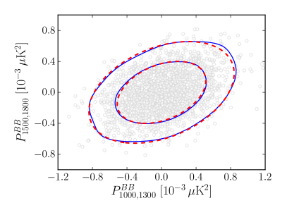
Fortunately for the likelihood construction, non-Gaussian covariances $\mathcal{N}_{\ell\ell^{\prime}}^{XY,WZ}$ of the low $\ell$ data are considerably smaller than the corresponding Gaussian part of the covariance. Indeed, the largest correlation coefficient

$$R^{XY,WZ}_{\ell\ell^{\prime}}=\frac{\mathcal{N}^{XY,WZ}_{\ell\ell^{\prime}}}{\sqrt{\mathrm{Cov}^{XY,XY}_{\ell\ell}\mathrm{Cov}^{WZ,WZ}_{\ell^{\prime}\ell^{\prime}}}}$$ (10)

with $\ell<30$ is $8\times 10^{-4}$. We shall therefore neglect lensing-induced covariances in the likelihood for the large scale data.

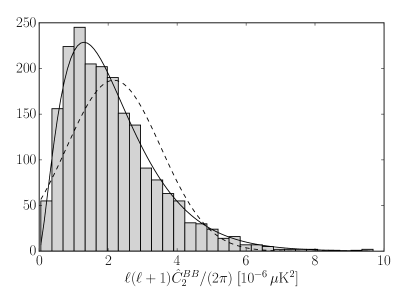
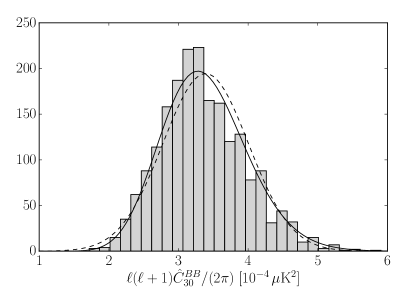
As pointed out above, the low $\ell$ data are not normally distributed. For example, in Fig. 2 we plot the distribution of $B$-mode power spectra including noise for $\ell=2,30$ obtained in the same Lenspix simulations. In the same plot we show a normal distribution centered on the expected mean of the data, with standard deviation given by the Gaussian expectation (3)

$$\sigma^{BB}_{\ell}=\sqrt{\frac{2}{2\ell+1}}C^{BB}_{\mathrm{exp},\ell}.$$ (11)

It is clear that for $\ell=2$ the normal distribution is a poor description of the data. Instead, as expected, $\chi^{2}_{2\ell+1}$ distribution scaled by $\sigma^{BB}_{\ell}$ fits the data well. In the case of large scale $B$-modes this reflects the fact that they get most of their power from $\tilde{E},\phi$ modes at $\ell$ of several hundred. Each coefficient in the spherical harmonic expansion of the $B$ map is then a combination of many random fields and thus approximately normally distributed, which leads to $\chi^{2}$ distributed power spectra. For low $\ell$ $TT,TE$ and $EE$, the distributions just mirror the unlensed CMB fields, due to negligible effects of lensing on these fields. Above $\ell\sim 30$ the normal distribution becomes a good description for both the $\chi^{2}$ distribution and the data.

Figure 2: Distribution of $\hat{C}^{BB}_{2},\hat{C}^{BB}_{30}$ obtained from 2000 Lenspix simulations compared against a $\chi^{2}$ distribution with the Gaussian variance $(\sigma^{BB}_{\ell})^{2}$ (solid) and a normal distribution with the same variance centered on the expected mean of the data (dashed). The normal distribution becomes a good approximation for $\ell\gtrsim 30$.

Based on these considerations, our model for the likelihood treats $\hat{C}_{\ell}^{XY}$ from the largest scales ($\ell<\ell_{\mathrm{break}}$) and from smaller scales separately and independently. The choice of the division point is somewhat arbitrary; in this work we use $\ell_{\mathrm{break}}=30$.

Below $\ell_{\mathrm{break}}$ we neglect lensing-induced covariance $\mathcal{N}^{XY,WZ}_{\ell,\ell^{\prime}}$ and assume there is no correlation between $B$ modes and $T,E$ modes. Data with different multipoles $\ell,\ell^{\prime}$ then decouple. The likelihood of measuring the data vector $\hat{C}_{\ell}^{XY}$ (including instrumental noise) when the expected power spectra are $C^{XY}_{\mathrm{exp},\ell}$ is then a product of inverse Wishart distributions

$$\mathcal{L}_{\ell<\ell_{\mathrm{break}}} \propto {\prod}_{\ell=2}^{\ell_{\mathrm{break}}-1}\left|C^{XY}_{\mathrm{exp},\ell}\right|^{-(2\ell+1)/2}$$

$$\times\exp\left(-\frac{{2\ell+1}}{2}\sum_{X,Y}\left(C_{\mathrm{exp},\ell}^{XY}\right)^{-1}{\hat{C}}^{XY}_{\ell}\right).$$

Here $|\cdot|$ is a determinant of $\cdot$ viewed as a matrix, here in the $X,Y$ space.

For $\ell\geq\ell_{\mathrm{break}}$ we neglect the non-normality of the distribution of each multipole and instead model the lensing-induced covariance between multipoles:

$$\mathcal{L}_{\ell\geq\ell_{\mathrm{break}}}\propto|\mathrm{Cov}|^{-{1/2}}$$

$$\exp\Bigg{[}-\frac{1}{2}\sum_{\begin{subarray}{c}\text{$\ell,\ell^{\prime}\geq\ell_{\mathrm{break}}$}\\ \text{$XY,WZ$}\end{subarray}}\Delta C^{XY}_{\ell}\left(\mathrm{Cov}^{XY,WZ}_{\ell,\ell^{\prime}}\right)^{-1}\Delta C^{WZ}_{\ell^{\prime}}\Bigg{]}.$$

In all analyses in this paper we neglect the dependence of the covariance matrix on the cosmological parameters by evaluating it at the fixed fiducial model of Tab. 1.

To assess the impact of non-Gaussian covariance, we also investigate the likelihood $\mathcal{L}_{\mathrm{g},\ell\geq\ell_{\mathrm{break}}}$ in which the non-Gaussian covariance $\mathrm{Cov}_{\ell,\ell^{\prime}}$ is replaced by the Gaussian covariance $\mathcal{G}_{\ell,\ell^{\prime}}$.

By joining the large and small scale portions independently, we then form the total likelihood for the data

$$\ln\mathcal{L}=\ln\mathcal{L}_{\ell<\ell_{\mathrm{break}}}+\ln\mathcal{L}_{\ell\geq\ell_{\mathrm{break}}}$$ (14)

and

$$\ln\mathcal{L}_{\mathrm{g}}=\ln\mathcal{L}_{\ell<\ell_{\mathrm{break}}}+\ln\mathcal{L}_{\mathrm{g},\ell\geq\ell_{\mathrm{break}}},$$ (15)

up to irrelevant additive constants.

By comparing analyses based on these two likelihoods we are able to gauge the impact of non-Gaussian covariance on parameter constraints. The lensing-induced covariance is an additional source of correlated noise so constraints based on the likelihood with Gaussian covariance are typically too optimistic.

III Cosmological parameter estimation

In this section we investigate how neglecting lensing-induced covariance affects constraints on cosmological parameters. We focus here on the six parameter flat $\Lambda$CDM cosmological model and two extensions where either the sum of the masses of neutrinos $\sum m_{\nu}$ ($\Lambda$CDM+$\sum m_{\nu}$) or the dark energy equation of state parameter $w$ ($\Lambda$CDM+$w$) is allowed to vary. Similar studies on the impact of non-Gaussian covariances have been previously performed mainly using the Fisher approximation Smith et al. (2006); Benoit-Levy et al. (2012); Motloch et al. (2017); Peloton et al. (2016). We find that in at least one case ($\Lambda$CDM+$w$) the Fisher approximation significantly underestimates the impact of lensing-induced covariance.

For $\Lambda$CDM we also illustrate how neglecting lensing-induced covariance leads to a significant increase in the fraction of realizations in which the fiducial model parameters are excluded at 95% confidence, which is potentially important for concordance studies.

III.1 $\Lambda$CDM

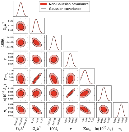
Neglecting lensing-induced covariances for a typical simulated CMB dataset affects constraints on $\Lambda$CDM parameters as shown in Fig. 3. Shifts in the best fit parameter values of the base parameters of Tab. 1 are typically not very significant; the major effect of including lensing covariances is a weakening of the best constrained directions between degenerate parameters, most notably that between $\Omega_{c}h^{2}$ and $A_{s}$. We comment on the origin of this effect in §IV.3.

Figure 3: Comparison of MCMC constraints on $\Lambda$CDM parameters with analysis based on Gaussian (black curves) and non-Gaussian covariance (red shaded). Here and throughout contours enclose regions of 68% and 95% confidence intervals unless otherwise specified.

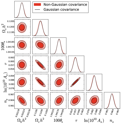
Because of marginalization of other parameters, the two parameter posteriors in Fig. 3 hide some of the effects of the non-Gaussian covariance. To uncover the maximal possible effect on a single quantity, we construct the linear combination of the cosmological parameters

$$M=\sum_{A}\mathcal{K}_{A}\left(\theta_{A}-\theta_{A}^{\mathrm{fid}}\right)$$ (16)

that maximizes the ratio of Gaussian to non-Gaussian errors. Here $\mathcal{K}_{A}=\{5.8,-13.4,18.4,-1.1,-2.6,3.1\}$ for the parameter ordering $\{{{100}\theta_{*}},{\Omega_{c}h^{2}},{\Omega_{b}h^{2}},{n_{s}},{{\ln A_{s}}},{\tau}\}$. As we discuss in greater detail in §IV.3, $M$ can be interpreted as a combination of cosmological parameters which mainly changes the lensing potential, especially at low $\ell$.

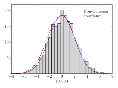
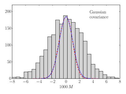
Dashed red lines in Fig. 4 show posterior probabilities for $M$, as determined from a single MCMC run based on $\mathcal{L}$ (left) and $\mathcal{L}_{\mathrm{g}}$ (right). The same simulated CMB sky as in Fig. 3 is used, the maximum has been shifted to zero for future convenience, and the $y$-axis units are arbitrary. The standard deviations of these two posteriors are $\sigma^{\mathrm{ng}}_{M}={2.1}\times 10^{-3}$ and $\sigma^{\mathrm{g}}_{M}={1.0}\times 10^{-3}$, both within 3% of the Fisher forecast prediction displayed in Fig. 4 by a solid blue line. The analysis based on a Gaussian likelihood $\mathcal{L}_{\mathrm{g}}$ therefore underestimates the errors of $M$ by over a factor of 2.

While the impact of this direction is hidden in the marginalized errors of the base parameters, it reveals itself in an increased frequency of Type 1 errors: falsely rejecting the true model. This effect would be particularly problematic for concordance studies searching for tensions between various cosmological datasets.

Figure 4: Histograms showing best fit values of $M$ determined from 2000 lensed CMB skies using an analytic approach (see text) for analysis based on non-Gaussian (left) and Gaussian covariance (right). The dashed red curves show the 1D posterior probability for $M$, as determined from a single CMB realization, shifted to zero for better comparison. Despite the Fisher forecast (solid blue curves) agreeing in both cases, the posterior probability does not reflect the much wider best-fit distribution in the Gaussian case.

Since a full study of Type 1 errors in thousands of data realizations is computationally expensive, we illustrate this problem by analytically approximating the best fit values of the parameters, including $M$, for each realization. We assume the data are sufficiently close to the fiducial model that it is possible to approximate the $C_{\ell}^{XY}$ as linear in the parameter deviations $\theta_{A}-\theta_{A}^{\rm fid}$. Neglecting for the moment complications arising from presence of the low $\ell$ data by assuming all the data are distributed according to a multivariate normal distribution with covariance (2), we obtain the maximum likelihood or best fit estimate for a cosmological parameter $\theta^{\mathrm{bf}}_{A}$ as

$$\Delta\theta_{A} \equiv \theta_{A}^{\mathrm{bf}}-\theta_{A}^{\mathrm{fid}}$$

$$= \sum_{\begin{subarray}{c}\text{$B,i,j$}\end{subarray}}F^{-1}_{AB}\frac{\partial D_{i}}{\partial\theta_{B}}\left(\mathrm{Cov}^{-1}\right)_{ij}\left(\hat{D}_{j}-D_{j}^{\mathrm{fid}}\right).$$

Here the power spectrum data are indexed as $D_{i}=C^{XY}_{\ell}$ with $i$ running over all $XY,\ell$ elements. The Fisher information matrix,

$$F_{AB}=\sum_{\begin{subarray}{c}ij\end{subarray}}\frac{\partial D_{i}}{\partial\theta_{A}}\left(\mathrm{Cov}\right)^{-1}_{ij}\frac{\partial D_{j}}{\partial\theta_{B}},$$ (18)

and parameter derivatives are evaluated around the fiducial model.

With the best fit values of cosmological parameters we can directly calculate the best fit values of $M$ for both the non-Gaussian and Gaussian analysis. The two differ only in the choice of covariance matrix in Eqs. (III.1) and (18).

Best fit values of $M$ determined from 2000 simulated CMB skies are shown in histograms in Fig. 4 for the non-Gaussian (left) and Gaussian (right) covariance analyses. In the non-Gaussian case, this distribution has a standard deviation $\sigma^{\mathrm{ng}}_{M,\mathrm{bf}}=2.1\times 10^{-3}$ which is in excellent agreement with the prediction from the posterior $\sigma^{\mathrm{ng}}_{M}$ determined from the MCMC analysis of single realization as well as the Fisher approximation. On the other hand, in the Gaussian analysis the best fit values of $M$ scatter with standard deviation $\sigma^{\mathrm{g}}_{M,\mathrm{bf}}=2.5\times 10^{-3}$, which is 2.5 times the width of $\sigma^{\mathrm{g}}_{M}$ despite the latter agreeing with its Fisher approximation. This mismatch can lead to Type 1 errors in cases where the best fit $M$ fluctuates away from the fiducial value zero.

Notice that the best fit distribution is wider in the Gaussian than non-Gaussian case by a factor of $\sim 1.2$ which further exacerbates the probability of Type 1 errors. This is not surprising, Eq. (III.1) is a minimum variance estimator only if the assumed model of the covariances is correct which it is not in the Gaussian case.

Figure 5: Histogram of $\chi^{2}(\Delta\theta_{A})$ for the parameter deviations of the best fit from the true model (19), as determined from our simulations with Gaussian (blue) and non-Gaussian (red) covariance. For comparison, the solid line is proportional to probability density function of $\chi^{2}_{6}$. The long tail in the Gaussian case leads to anomalously frequent Type 1 errors where the true model is rejected at high confidence (see text).

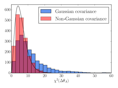
To quantify the probability of Type 1 errors considering all parameters that specify the $\Lambda$CDM model, we can also compute $\chi^{2}$ between the best fit and the true fiducial model assuming the errors from the posterior

$$\chi^{2}(\Delta\theta_{A})=\sum_{AB}\Delta\theta_{A}{\rm Cov}_{AB}^{-1}\Delta\theta_{B}\approx\sum_{AB}\Delta\theta_{A}F_{AB}\Delta\theta_{B}.$$ (19)

In order to estimate $\chi^{2}$ for each of the 2000 lensed CMB simulations, we again use the Fisher matrix as an approximation to the inverse covariance. The variable $\chi^{2}(\Delta\theta_{A})$ should be $\chi^{2}_{6}$ distributed, where 6 is the number of cosmological parameters in $\Lambda$CDM.

Histograms of $\chi^{2}(\Delta\theta_{A})$ for the Gaussian and non-Gaussian analysis are compared in Fig. 5 to the theoretical expectation. It is clear that in the Gaussian analysis, the misestimate of the parameter covariance as well as the suboptimal estimate of the best fit causes a strong disagreement with the expected $\chi^{2}_{6}$ distribution.

For example, when the analysis is based on the Gaussian covariance, more than 30% of the simulations show $\chi^{2}(\Delta\theta_{A})>12.59$; for $\chi^{2}_{6}$ this value is exceeded only in 5% of the cases. As pointed out above, this can be potentially dangerous for concordance studies. The non-Gaussian covariance leads to much better agreeement ($\sim$ 6.9% of simulations have $\chi^{2}(\Delta\theta_{A})>12.59$) and moreover there is no long tail to very high $\chi^{2}(\theta_{A})$.

In the Appendix B we comment on small changes to some of the conclusions of this section for an experimental configuration which observes only part of the sky and does not measure data at multipoles $\ell<30$.

III.2 $\Lambda$CDM + $\sum m_{\nu}$

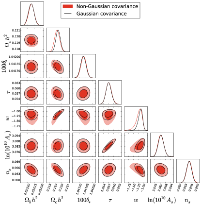
In this section we release the neutrino mass from its fiducial value and investigate a seven-parameter extension of $\Lambda$CDM. In this case, the two parameter contour plots, shown in Fig. 6, show much smaller effects of non-Gaussian covariance than in $\Lambda$CDM, though the impact is visible in the lower limit for $\sum m_{\nu}$. Ref. Peloton et al. (2016) also found only small effects for this case.

Figure 6: Comparison of MCMC constraints on $\Lambda$CDM+$\sum m_{\nu}$ parameters with analysis based on Gaussian (black curves) and non-Gaussian covariance (red shaded).

However, this does not mean non-Gaussian covariance can be neglected in this case, only that its effects are hidden by marginalizations. As for $\Lambda$CDM, we can form a combination of the cosmological parameters which is predicted by the Fisher forecast to show the largest effect of non-Gaussian covariance,

$$M^{\nu}=\sum_{A}\mathcal{K}^{\nu}_{A}\left(\theta_{A}-\theta_{A}^{\mathrm{fid}}\right)$$ (20)

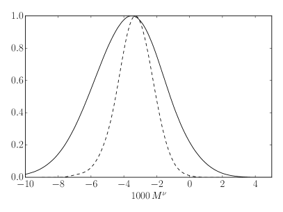
with $\mathcal{K}^{\nu}_{A}=\{5.7,-13.3,18.4,-1.1,-2.6,3.1,0.29\,\mathrm{eV}^{-1}\}$, for the ordering $\{{{100}\theta_{*}},{\Omega_{c}h^{2}},{\Omega_{b}h^{2}},{n_{s}},{{\ln A_{s}}},{\tau},{\sum m_{\nu}}\}$. In Fig. 7 we can see 1D posterior probabilities for $M^{\nu}$ from MCMC analyses based on Gaussian and non-Gaussian covariance. It is clear $M^{\nu}$ constraints are nearly as strongly affected by the lensing-induced covariance as $M$ for $\Lambda$CDM, with standard deviation degrading from $1.1\times 10^{-3}$ to $2.2\times 10^{-3}$, even though this effect does not show up in any pair of base parameters. Likewise, the Gaussian analysis is prone to Type 1 errors as in the $\Lambda$CDM case.

The standard deviations of $M^{\nu}$ quoted in the previous paragraph differ somewhat from their Fisher forecasts: $1.0\times 10^{-3}$ and $2.1\times 10^{-3}$ for the Gaussian and non-Gaussian cases respectively. This occurs in part because the posterior is non-normal due to the presence of the physicality prior $\sum m_{\nu}>0$ which hides some of the non-Gaussian covariance effects (cf. Fig. 6). In cases where neutrino mass is detected with high significance and effects of the prior boundary is smaller, $M^{\nu}$ constraints are in good agreement with the Fisher prediction.

Figure 7: Effect of the non-Gaussian covariance on constraints on a parameter combination $M^{\nu}$ (20) within $\Lambda$CDM+$\sum m_{\nu}$; the combination was chosen to maximize this effect. Solid line shows MCMC constraints with non-Gaussian covariance, dashed line with the Gaussian covariance.

III.3 $\Lambda$CDM + $w$

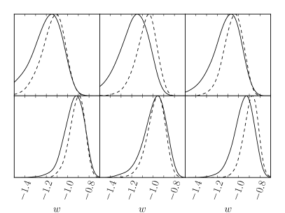
In the model where we allow the dark energy parameter of state to vary, the effect of non-Gaussian covariance is more pronounced and clearly visible already on posterior probability distribution for $w$, see Fig. 8. The two analyses, based on $\mathcal{L}$ and $\mathcal{L}_{\mathrm{g}}$, strongly disagree in the low $w$ tail; by neglecting the covariance induced by the gravitational lensing one would wrongly rule out low values of $w$. For example, for this particular realization lower 95% confidence limits (two sided) for the non-Gaussian and Gaussian likelihoods are $-1.55$ and $-1.37$ respectively. In §IV.3 we look deeper into this behavior.

The impact of non-Gaussian covariance depends to some extent on best fit value of $w$; simulations with lower best fit value of $w$ typically show larger effects of non-Gaussian covariance. To illustrate this, in Fig. 9 we show marginalized constraints on $w$ for six different simulations, both with Gaussian and non-Gaussian likelihood.

In the Fisher approximation, $\Lambda$CDM+$w$ was investigated for essentially the same experimental configuration in Smith et al. (2006). It was found that non-Gaussian covariances should increase errors on $w$ by only about 24%, which is considerably less than what we uncovered in the full MCMC analysis. In this case, the local approximation thus gives misleading results, due to the non-normal posterior which the Fisher approximation can not faithfully capture. The origin of this behavior can be traced back to how dark energy affects lensing. As $w$ decreases, its effect on the lensing potential quickly diminishes, as dark energy ceases to be important at redshifts where the lensing kernel peaks. Because in this case the parameter combination constrained by lensing is significantly changing throughout the allowed parameter posterior, the Fisher analysis fails to capture the full significance of the non-Gaussian covariance.

Figure 8: Comparison of MCMC constraints on $\Lambda$CDM+$w$ parameters with analysis based on Gaussian (black curves) and non-Gaussian covariance (red shaded). The impact of non-Gaussian covariance is clearly apparent in constraints involving $w$.

Figure 9: Comparison of MCMC constraints on $w$ for our experimental setup; each panel represents a different $\Lambda$CDM simulation of the CMB sky with that of Fig. 8 in the top left corner. The Gaussian analysis (dashed) increasingly deviates from the non-Gaussian analysis (solid) as the maximum likelihood value of $w$ decreases.

The maximally impacted linear combination of base parameters also shows an enhanced non-Gaussian effect compared with $\Lambda$CDM and $\Lambda$CDM+$\sum m_{\nu}$. It reads

$$M^{w}=\sum_{A}\mathcal{K}^{w}_{A}\left(\theta_{A}-\theta_{A}^{\mathrm{fid}}\right),$$ (21)

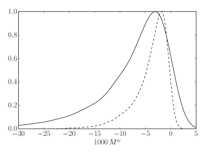
where $\mathcal{K}^{w}_{A}=\{5.7,-12.8,18.0,-1.0,-2.5,2.9,0.087\}$ for the ordering $\{{{100}\theta_{*}},{\Omega_{c}h^{2}},{\Omega_{b}h^{2}},{n_{s}},{{\ln A_{s}}},{\tau},{w}\}$. Posterior probabilities for $M^{w}$ from MCMC analyses based on Gaussian and non-Gaussian covariance are shown in Fig. 10. In this case, the standard deviations $\sigma^{\mathrm{ng}}_{M^{w},\mathrm{Fish}}=2.3\times 10^{-3}$ and $\sigma^{\mathrm{g}}_{M^{w},\mathrm{Fish}}=1.0\times 10^{-3}$ derived using a Fisher approximation show that the relative impact of non-Gaussian covariance is in reasonable agreement with the MCMC results $\sigma^{\mathrm{ng}}_{M^{w}}=7.6\times 10^{-3}$ and $\sigma^{\mathrm{g}}_{M^{w}}=3.4\times 10^{-3}$, but the overall scale is still strongly underestimated by the Fisher analysis as is the extent of the lower tail. These mismatches are expected for the same reason that they appear in $w$ alone, namely due to parameter nonlinearity within the allowed region. Likewise, $M^{w}$ defined by (21) only captures the parameter combination which is the most affected by the lensing-induced covariance locally at the fiducial model parameters, not necessarily globally (see §IV.3).

Figure 10: Effect of the non-Gaussian covariance on constraints on a parameter combination $M^{w}$ (21) within $\Lambda$CDM+$w$; the combination was chosen to maximize this effect locally around the fiducial model. Solid line shows MCMC constraints with non-Gaussian covariance, dashed line with the Gaussian covariance.

IV Lens principal components

The temperature and polarization power spectra contain more information about the lensing potential than just its amplitude; this information can be faithfully captured in terms of a few principal components (PCs) Motloch et al. (2017); Smith et al. (2006). This model-independent lensing information can be utilized in a variety of ways. By isolating the lensing information, we can more directly diagnose when lensing-induced covariance is important for parameter constraints. Lensing PCs also enable us to check the internal consistency of the data with a given model, by comparing the constraints on parameters derived from the lensing potential with those from the unlensed power spectra. Comparing $C^{\phi\phi}_{\ell}$ constraints from the power spectra with those from the reconstructed lensing potential and external measurements provides yet another powerful consistency check. Finally, PCs enable model building beyond the currently considered model classes should these consistency tests fail.

In this section we conduct an MCMC study of the lensing PCs $\Theta^{(i)}$ as defined by the Fisher approximation Motloch et al. (2017); Smith et al. (2006) together with variables $\tilde{\theta}_{A}$ that parametrize the unlensed power spectrum. Since the PCs are defined under the Fisher approximation, we first verify that in the MCMC analysis the PCs remain unbiased and weakly correlated – both mutually and with $\tilde{\theta}_{A}$. Then we point out that almost the whole effect of the non-Gaussian covariance is manifested in the first two PCs $\Theta^{(1)},\Theta^{(2)}$ and use this knowledge to explain effects of non-Gaussian covariances on parameter constraints seen in the previous section.

We end this section with a discussion of possible consistency checks using these principal components and a suggestion of how to use them to compress most of the information contained in the lensed CMB power spectra into a simple normal likelihood, which can be used to quickly determine approximate constraints on a wider class of models than explicitly analyzed here.

Figure 11: Five principal components $K_{\ell}^{(i)}$ of the lensing potential best measured by the lensed power spectra.

IV.1 Parameterizing lens and unlensed power spectra

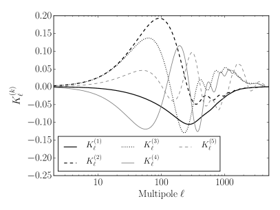
For a particular experiment and fiducial model, a Fisher forecast can determine which principal components $\Theta^{(i)}$ of $C_{\ell}^{{\phi\phi}}$ will be the best measured by the $XY$ power spectra. These PCs can be ordered by increasing variance so that only the handful of best measured components need be included in the actual analysis. In Ref. Motloch et al. (2017), the hierarchy of $\Theta^{(i)}$ was found for the experimental configuration considered here. These principal components are defined as

$$\Theta^{(i)}=\sum_{\ell}K^{(i)}_{\ell}(\ln C^{\phi\phi}_{\ell}-\ln C_{\ell}^{{\phi\phi},{\rm fid}}),$$ (22)

where $C^{{\phi\phi},{\rm fid}}_{\ell}$ is a fixed lensing potential, evaluated at the fiducial parameters given in Table 1. The lensing PCs, $\Theta^{(i)}$, can be thought of as a more incisive generalization of the standard approach where a scaling parameter $C_{\ell}^{\phi\phi}\rightarrow A_{L}C_{\ell}^{\phi\phi}$ is added to test consistency of a model with lensing; PCs parametrize the lensing information more completely. For reasons detailed in Appendix C, the 5 best measured PCs suffice for the data and models considered here; their weights $K^{(i)}_{\ell}$ are shown in Fig. 11.

Moreover, the PCs decouple the information on the lensing power spectrum from the parameters that control the unlensed spectrum, whereas $A_{L}$ multiplies a $C_{\ell}^{\phi\phi}$ that depends on such parameters. PCs can therefore be more directly compared with other measurements of $C_{\ell}^{\phi\phi}$, most notably from lensing reconstruction using the higher point information in the temperature and polarization fields themselves.

For example, in a cosmology where the unlensed power spectra fluctuate low but the lensing potential is consistent with the underlying model, there will be a tendency for high $A_{L}$: the unlensed CMB will drive the amplitude of fluctuations $A_{s}$ down, which will at the same time lower the amount of lensing predicted. To match the amount of lensing present in the data, $A_{L}$ or similar lensing parameter is then increased. Hence measuring a high $A_{L}$ does not necessarily signal a deviation in $C_{\ell}^{\phi\phi}$ itself.

In the PC approach, the unlensed CMB is described by separate parameters $\tilde{\theta}_{A}$. For models that modify only the low redshift physics involved in the growth of structure and cosmic acceleration it is sufficient to take these to be the equivalent of the six $\Lambda$CDM parameters. These $\tilde{\theta}_{A}$ change the unlensed power spectra in exactly the manner of the $\Lambda$CDM parameters, but unlike those, they have no effect on $C^{{\phi\phi}}_{\ell}$.

To summarize, CMB power spectra $C^{XY}_{\ell}$ can be effectively parameterized in terms of eleven parameters $\tilde{\theta}_{A}$ and $\Theta^{(i)}$ in any model that deviates from $\Lambda$CDM only after recombination, with $i={1-5}$ sufficing for the data and models we study. In this setup, $\Theta^{(i)}$ represent direct, optimally weighted, measurements of the lensing potential.

Figure 12: Joint posterior distribution for PCs $\Theta^{(1-5)}$ (black) as a product of the individual posteriors from 50 independent all-sky simulations. The joint posterior is unbiased to a small fraction of the width of the distribution of a single simulation (blue) and its Fisher prediction (red dashed).

IV.2 MCMC analysis of lens and unlensed parameters

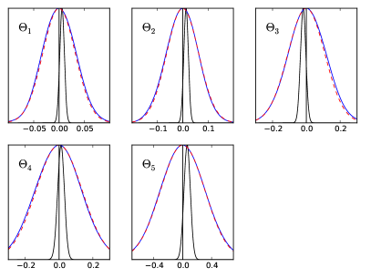
We run MCMC analyses on 50 independent lensed CMB sky simulations to check our likelihood model and to determine properties of the parameters $\tilde{\theta}_{A},\Theta^{(i)}$.

So far we have made numerous assumptions, for example that our models for the likelihood and non-Gaussian covariance are correct, that the Fisher-based construction of the PCs suffices, that neglecting higher $\Theta^{(i)}$ does not affect the constraints and that agreement between theoretical and simulated power spectra is sufficient (see Appendix A). It is thus a nontrivial check of our analysis to ascertain that the constraints on $\Theta^{(i)},\tilde{\theta}_{A}$ are unbiased with respect to the fiducial model. To check this, we multiplied 50 MCMC posterior probabilities for $\Theta^{(i)},\tilde{\theta}_{A}$. The results for $\Theta^{(i)}$ are shown in Fig. 12 and show no significant bias relative to the standard deviation of a single MCMC posterior; the same conclusion is valid also for $\tilde{\theta}_{A}$.

Figure 13: Correlation matrix for $\Theta^{(i)}$ averaged over 50 MCMC analyses. Black squares represent ones on the diagonal. The tilded parameters affect only the unlensed CMB, as explained in the text.

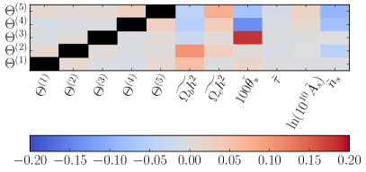
The Fisher analysis also predicts that $\Theta^{(i)}$ as determined by the data should be uncorrelated. This assertion can be checked by averaging covariance matrix of the cosmological parameters $\Theta^{(i)},\tilde{\theta}_{A}$ over the MCMC analyses. Correlation coefficients of $\Theta^{(i)}$ obtained from this covariance matrix are shown in Fig. 13. As expected, the lensing principal components are only very weakly mutually correlated. Additionally, they are also only mildly correlated with the unlensed parameters $\tilde{\theta}_{A}$. Most significant of these are $R=0.18$ correlation between $\Theta^{(3)}$ and $\theta_{*}$ and $R=-0.14$ correlation between $\Theta^{(4)}$ and $\theta_{*}$. This is somewhat counterintuitive, as $\theta_{*}$ shifts the angular scale of acoustic features whereas lensing mainly smears the peaks by superimposing magnified and demagnified regions. While largely true, the effect of lenses that are on scales smaller than the acoustic scale $\ell\gtrsim 200$ is not purely a smearing effect, causing a component that is slightly out of phase with the peaks in the unlensed power spectra, leading to the observed correlation.

Figure 14: MCMC constraints on the lens and unlensed parameters $\Theta^{(i)},\tilde{\theta}_{A}$ in a typical simulation with a Gaussian (black curves) and non-Gaussian covariance (red shaded) analysis.

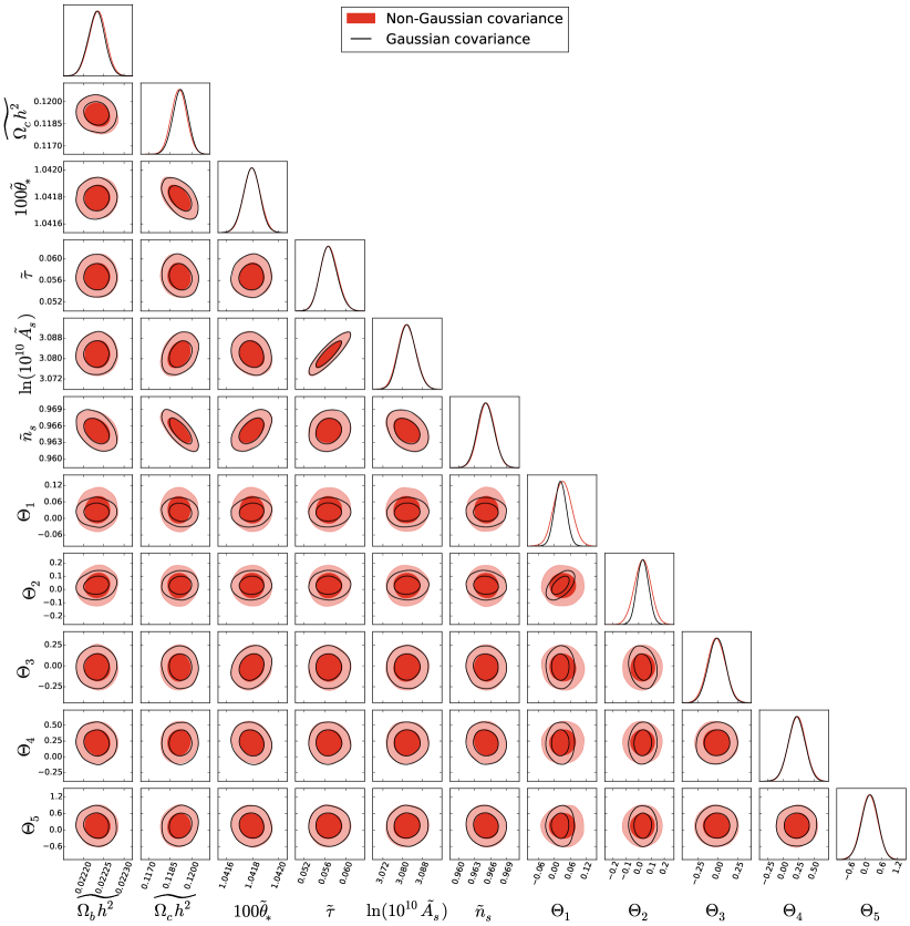
The full results for all pairs of the 11 parameters in a single simulation are shown in Fig. 14. Note that posterior distribution for the parameters $\Theta^{(i)},\tilde{\theta}_{A}$ seems to be very well approximated by a multivariate normal distribution. This implies that the Fisher approximation should be quite accurate in this space as we explicitly verify in Fig. 12. We exploit the multivariate normal nature of the posterior in the $\Theta^{(i)},\tilde{\theta}_{A}$ variables in the following sections.

IV.3 Impact of lensing-induced covariance revisited

In Fig. 14 we also show the effect of the non-Gaussian covariance in the 11D lens and unlensed parameter space; only $\Theta^{(1)}$ and $\Theta^{(2)}$ show significant effects of neglecting the non-Gaussian likelihood. These two measurements are strongly affected, because significant portion of the noise in these measurements arises from the sample variance of the lenses. Neglecting lensing-induced terms in the data covariance effectively omits this noise contribution, which leads to overly optimistic estimates on $\Theta^{(1)},\Theta^{(2)}$. Measurements of other lensing principal components and $\tilde{\theta}_{A}$ are limited by other sources of noise – instrumental noise and cosmic variance of the unlensed CMB – and the resulting constraints are thus not strongly affected by the non-Gaussian part of the covariance.

If the eleven parameters $\Theta^{(i)},\tilde{\theta}_{A}$ contain all information about a particular cosmological model, a Karhunen-Loève analysis applied to the Fisher information matrices Smith et al. (2006) reveals that non-Gaussian covariances can degrade the standard deviation of any linear combination of these parameters by maximally 2.53. This generalizes the discussion of the most degraded linear combination $M$ of cosmological parameters from §III. This PC based quantification of the effect of non-Gaussian covariances is not restricted to the models investigated here and can be applied to more general extensions of $\Lambda$CDM. It is also not necessary to assume a linear relationship between these effective parameters and the bare cosmological parameters, or the validity of the Fisher approximation for the latter.

Moreover, we can use $\Theta^{(1,2)}$ to directly translate the effect of lensing-induced covariance on cosmological parameter constraints. Those combinations of cosmological parameters which are limited by our knowledge of $\Theta^{(1,2)}$, in other words those constrained by the (mostly low $\ell$) lensing information, will be strongly affected if we neglect the non-Gaussian covariance.

For example in $\Lambda$CDM, lensing information helps mainly $\omega_{c}$ and $A_{s}$ constraints. Increasing either of these parameters increases $C^{\phi\phi}_{\ell}$, lensing information thus helps constrain the direction of simultaneously increasing $\omega_{c}$ and $A_{s}$. As we can see in Fig. 3, adding non-Gaussian covariance weakens exactly this parameter combination the most. The reason becomes clear when we examine how change in the parameter combination $M$, the most sensitive to the non-Gaussian covariances, projects onto the changes in the effective parameters $\Delta\Theta^{(i)},\Delta\tilde{\theta}_{A}$. As expected, the main effect is a shift in $\Theta^{(1)},\Theta^{(2)}$, which are the variables showing most of the effect of the non-Gaussian covariance; this shift is captured in Fig. 15. In comparison, shifts in the other effective parameters $\Theta^{(i)},\tilde{\theta}_{A}$ are at least a factor of few smaller, as measured by the sizes of the marginalized posterior. This means that already within $\Lambda$CDM it is possible to construct a parameter combination which has a dominant effect of changing the lensing potential ($\Theta^{(1)},\Theta^{(2)}$) and keeps the unlensed power spectra ($\tilde{\theta}_{A}$) relatively intact. Because of that, the relative change in the standard deviation for $M$ brought about by the non-Gaussian covariance 2.03 is already close to the maximal possible value of 2.53.

Figure 15: Lines show how $\Theta^{(1)}$ and $\Theta^{(2)}$ change when we increase $M$ (black dashed), $M^{\nu}$ (green) or $M^{w}$ (black solid); length of the lines is arbitrary. For comparison, in the background we show typical constraints on these two parameters in an MCMC analysis based on non-Gaussian (red) and Gaussian (blue) covariance.

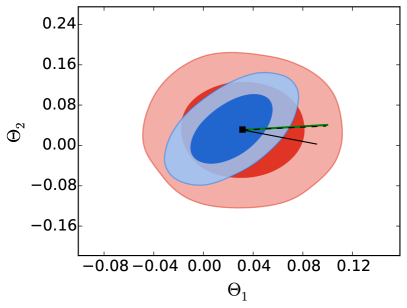
By extending the cosmological model to $\Lambda$CDM+$\sum m_{\nu}$, we increase the parameter freedom, which enables us to find a parameter combination which is slightly more limited by the lens sample covariance and shows degradation of 2.05. From the perspective of the effective parameters $\Theta^{(i)},\tilde{\theta}_{A}$ this occurs because it is possible to achieve the same change of the lensing potential, as seen in the nearly identical directions of $M$ and $M^{\nu}$ in Fig. 15, with a smaller change in the unlensed power spectra. This increases relative importance of the low $\ell$ lensing information $\Theta^{(1)},\Theta^{(2)}$ in constraining $M^{\nu}$, which directly leads to a larger impact of non-Gaussian covariance.

Moreover, lensing information is now important for three parameters $\{\omega_{c},A_{s},\sum m_{\nu}\}$ unlike two in $\Lambda$CDM. Because the degeneracy structure involves three parameters, the non-Gaussian effect is hidden from the covariance of any two, once the third is marginalized. In a three-dimensional likelihood for these three parameters, the effect of non-Gaussian covariance is clearly visible.

For $\Lambda$CDM+$w$ the analysis is similar. Again, by adding a new parameter on top of $\Lambda$CDM we can find $M^{w}$ which shows degradation larger than what is seen in $\Lambda$CDM, in this case 2.28. For $\Lambda$CMD+$w$ this happens, because the projection of $M^{w}$ onto $\{\Theta^{(1)},\Theta^{(2)}\}$ is more aligned with the direction maximally impacted by the non-Gaussian covariance, see Fig. 15.

IV.4 Consistency tests

The simplest lensing consistency test of a model is to compare lensing potential measured through $\Theta^{(i)}$ against what is expected based on the cosmological model determined by constraints on the unlensed power spectra $\tilde{\theta}_{A}$. This test mainly checks the internal consistency of the model assumptions.

If there are also additional measurements of the lensing potential, then a sharper consistency check is possible Motloch et al. (2017). A certain linear combination of the power spectrum PCs,

$$\Psi^{(1)}=\sum_{i=1}^{5}\mathcal{T}_{i}\Theta^{(i)}$$ (23)

with $\mathcal{T}_{i}=\{32.3,-15.9,0.330,1.72,-0.608\}$, is predicted by the Fisher analysis to be limited mainly by lens sample variance, which drops out when comparing with other measurements on the same patch of sky leaving a nearly noise-free consistency test. This consistency test therefore checks for systematics in the data analysis, foregrounds, and assumptions about the unlensed power spectra.

In Fig. 16, we illustrate this idea explicitly by comparing posterior mean values of $\Psi^{(1)}$ determined from 50 simulated power spectra using MCMC against values of $\Psi^{(1)}$ determined directly from a known realization of the lensing potential, which can be thought of as a limiting case of lensing potential measurement with no instrumental noise. The latter approach estimates $\Theta^{(i)}$ from simulated $C_{\ell}^{\phi\phi}$ using an unbiased estimator

$$\Theta^{(i)}_{\mathrm{est}}=\sum_{\ell}K^{(i)}_{\ell}(\ln C^{\phi\phi}_{\ell}-\langle\ln C_{\ell}^{{\phi\phi}}\rangle),$$ (24)

where $\langle\cdot\rangle$ is expectation value over realizations, and combines the results according to (23). The observed correlation is indeed very tight; residual scatter in Fig. 16 is caused by instrumental noise and variance of the unlensed CMB which affect the power spectrum measurement.

Figure 16: Consistency mode $\Psi^{(1)}$ as determined from posterior mean values in 50 simulated lensed power spectra through MCMC analysis against values determined from known realizations of the lensing potential (see text for details). The dashed line represents points where the two determinations are equal.

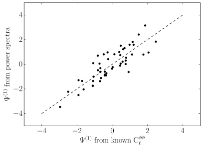
Notice also that this direction is mainly composed of $\Theta^{(1)}$ and $\Theta^{(2)}$ in nearly the same combination that is maximally affected by non-Gaussian lens sample variance. While being limited by the lens sample variance is detrimental to cosmological parameter constraints, for consistency tests this is advantageous because lens sample variance drops out when comparing measurements on the same patch of sky.

There is also another combination of PCs, $\Psi^{(2)}$,

$$\Psi^{(2)}=\sum_{i=1}^{5}\mathcal{U}_{i}\Theta^{(i)}$$ (25)

with $\mathcal{U}_{i}=\{31.3,17.6,10.4,0.945,-1.10\}$, which can serve as a similar consistency check; this consistency check is slightly weaker than the test using $\Psi^{(1)}$ due to the larger impact of noise and sample variance of the unlensed CMB. This weakening can be seen in Fig. 17, where we compare values of $\Psi^{(2)}$ determined from 50 simulated power spectra against values from known realization of the lensing potential.

Figure 17: Same as Fig. 16 but for the consistency mode $\Psi^{(2)}$.

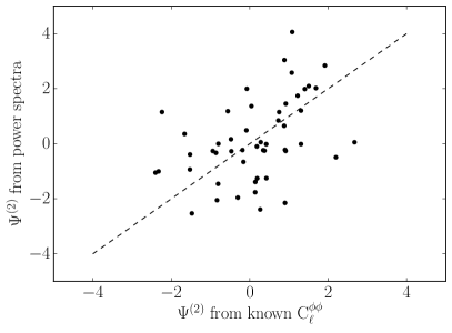
Notice also that there is no indication of bias in the power spectrum estimate of the two consistency modes in Figs. 16, 17. To better quantify this, in Figure 18 we show product of 50 posteriors for measurements of $\Psi^{(1)},\Psi^{(2)}$ as determined from our MCMC simulations and the determination is indeed unbiased; from the power spectra side there does not seem to be any problem for the consistency check.

Figure 18: Joint posterior of the consistency parameters $\Psi^{(1)},\Psi^{(2)}$ (black) as the product of 50 individual posterior distributions from independent all-sky simulations. Compared against the width of a single posterior (blue) there is no indication of bias with respect to the fiducial value $\Psi^{(i)}=0$ at a fraction of the standard deviation.

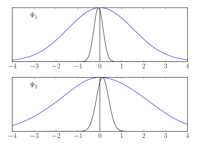
We also find that $\Psi^{(1)}$ is almost uncorrelated with the $\Lambda$CDM parameters describing the unlensed power spectra; the largest correlation coefficient we find is $R=-0.03$ and occurs between $\Psi^{(1)}$ and $\widetilde{\Omega_{b}h^{2}}$. The other consistency mode is slightly more correlated with the unlensed parameters; the most correlated with $\Psi^{(2)}$ are $\tilde{\theta}_{*}$ with correlation coefficient $R=0.12$ and $\widetilde{\Omega_{b}h^{2}}$ with $R=0.08$.

Failure of the consistency check could indicate an unlensed spectrum that is not described by the flat $\Lambda$CDM parameters. In fact in Motloch et al. (2017) it was shown that the second consistency mode $\Psi^{(2)}$ is correlated with the spatial curvature given their similar effects on the acoustic peaks. We run a single MCMC analysis in which we added $\tilde{\Omega}_{K}$ to the unlensed parameters and confirm this finding; there is a strong correlation between $\tilde{\Omega}_{K}$ and $\Psi^{(2)}$ with correlation coefficient $R=-0.62$. In a non-flat Universe analyzed as flat this would lead to failure in the consistency check as $\Psi^{(2)}$ would move from its true value to absorb the unaccounted for curvature. The main consistency mode, $\Psi^{(1)}$, is correlated with $\tilde{\Omega}_{K}$ at the $R=0.29$ level and is a weaker check on curvature.

IV.5 Effective Likelihood for Model Building

Given the nearly multivariate normal posterior probability of the effective parameters $d_{a}=\{\tilde{\theta}_{A},\Theta^{(i)}\}$, we can also use a single MCMC analysis to compress the whole CMB power spectra data into 11 numbers for the mean values $\bar{d}_{a}$ and the $11\times 11$ covariance matrix of $d_{a}$. These can be used to form an effective likelihood function ${\cal L}_{\rm eff}(\bar{d}_{a}|\theta_{A})$ defined as

$$-2\ln{\cal L}_{\rm eff}=\sum_{ab}[\bar{d}-d(\theta_{A})]_{a}({\rm Cov}_{d}^{-1})_{ab}[\bar{d}-d(\theta_{A})]_{b}.$$ (26)

Here $d_{a}(\theta_{A}$) models the expectation values for the data $\bar{d}_{a}$ as a function of the cosmological parameters $\theta_{A}$ of a given cosmological model. This effective likelihood can be now used to probe a broad class of cosmological models without any explicit use of the raw CMB power spectra data by specifying $d_{a}(\theta_{A})$ for each such model. Class of models for which this approach is effective contains not just $\Lambda$CDM+$w$ and $\Lambda$CDM+$\sum m_{\nu}$ considered here but also models which are indistinguishable from $\Lambda$CDM at recombination and for which CMB lensing is the dominant source of information on the physics beyond $\Lambda$CDM. For example, many models of dark energy and modified gravity fall into this class, if we are willing to ignore the extra information coming from the integrated Sachs-Wolfe effect and other secondaries. In principle, the technique can be extended to incorporate such effects by extending the set of unlensed parameters $\tilde{\theta}_{A}$.

In the context of model building, one can envision a scenario where $\Lambda$CDM parameters produce a poor effective likelihood for the data and motivate extensions beyond $\Lambda$CDM. The effective likelihood can then be used as a quick spot check as to whether the given extension improves the fit.

Let us illustrate this technique on $\Lambda$CDM+$w$ and $\Lambda$CDM+$\sum m_{\nu}$. First, it is necessary to find the functional dependence of $d_{a}$ on the cosmological parameters $\theta_{A}$. The values of the unlensed parameters $\tilde{\theta}_{A}$ for $A\in\{{\theta_{*}},{\Omega_{c}h^{2}},{\Omega_{b}h^{2}},{n_{s}},{{\ln A_{s}}},{\tau}\}$ are the same as the true cosmological parameters $\theta_{A}$, while the values of the lensing principal components $\Theta^{(i)}$ can be determined directly from the definition (24) given $C_{\ell}^{\phi\phi}$ alone. The full parameter space of the given extension can then be explored with an MCMC in the general case where $d_{a}(\theta_{A})$ is nonlinear across the allowed region of the parameter space as in the $\Lambda$CDM+$w$ extension. In a case such as $\Lambda$CDM+$\sum m_{\nu}$, where the mapping can be linearized, it is possible to get a good estimate of parameter constraints even without performing any additional MCMC.

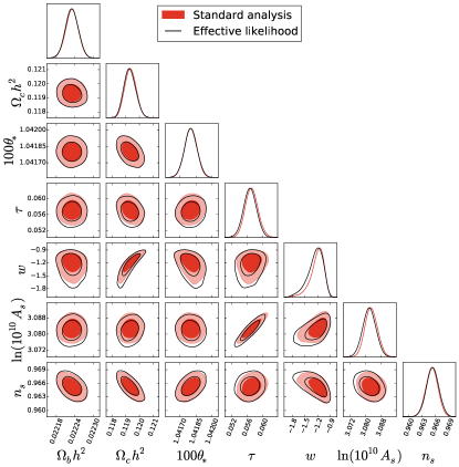
In Fig. 19 we show comparison of $\Lambda$CMD+$w$ parameter constraints obtained in the analysis presented in the previous paragraph against results of the standard MCMC analysis. Because the mapping onto the effective parameter space is non-linear, it is necessary to perform an additional MCMC run. Note that this mapping alone accounts for most of the non-normal posterior probability in the $(\omega_{c},w)$ plane despite being based on a normal distribution for the effective parameters. It slightly underestimates the lower limit on $w$, presumably due to the neglect of the integrated Sachs-Wolfe effect in the unlensed parameters. For $\Lambda$CDM+$\sum m_{\nu}$, the agreement between the simplified and standard analyses is even better.

Figure 19: Comparison of constraints on $\Lambda$CDM+$w$ parameters from the standard analysis (red shaded) with results of an approximate analysis based on the effective likelihood of $\{\Theta^{(i)},\tilde{\theta}_{A}\}$ instead of the raw CMB data (black).

V Discussion

Future measurements of lensed CMB power spectra will be increasingly affected by the lens sample variance and its effect on parameter constraints will have to be included into the analysis pipelines once polarization measurements approach the sample variance limit. To this end we have developed and tested such an analysis pipeline starting from simulated lensed maps with CMB-S4 level instrument noise through to constraints on cosmological parameters and the lens power spectrum.

The first piece in the pipeline is a model for the likelihood function of full-sky lensed CMB power spectrum data, which includes the non-Gaussian effects of lensing sample variance that correlate the measurements. This model considers large and small multipole data as independent. At small multipoles, the likelihood assumes data are Wishart distributed and drops the small non-Gaussian effects of lensing, while at large multipoles it assumes they are multivariate-normal distributed, with a covariance matrix which includes the lensing correlation across multipole moments.

With this likelihood we investigated parameter constraints from simulated lensed CMB maps of a fiducial $\Lambda$CDM model. We obtain MCMC parameter constraints on the $\Lambda$CDM parameters as well as two extensions, $\Lambda$CDM+$\sum m_{\nu}$ and $\Lambda$CDM+$w$. The dominant effect of the lensing-induced covariance in all of the models is more than four-fold increase in variance of particular combinations of cosmological parameters $M,M^{\nu},M^{w}$. As a consequence, if the analysis of the real data was performed using Gaussian covariance in the likelihood, instead of the proper non-Gaussian covariance, there is a high chance of committing Type 1 error - mistakenly ruling out true cosmological model. This would potentially affect concordance studies comparing constraints from various datasets. Shifts in the best fit basis parameters and change in constraints of the other parameter combinations are typically not as significant due to marginalization. The exception is $\Lambda$CDM+$w$ where a significant degradation in the lower limit for $w$ is manifest in the MCMC results. This degradation is hidden from the local Fisher forecasts as well as previous studies due to the strongly non-normal posterior distribution of $w$.

Then we explored the use of direct constraints on the lensing potential through a principal component analysis. Here eleven parameters effectively describe most of the cosmological information contained in the lensed CMB power spectra. Five of these parameters, $\Theta^{(i)}$, are the best measured principal components of the lensing potential while the remaining six, $\tilde{\theta}_{A}$, parameterize the unlensed power spectra. Measurement of $\Theta^{(i)}$ from data are well suited for various consistency tests involving measurements of the lens power spectrum. This should be contrasted with the standard approach where cosmological parameters are augmented by a scaling parameter $A_{L}$ to the lens power spectrum but the latter itself depends on cosmological parameters which are subsequently marginalized. Here the measured $\Theta^{(i)}$ can be compared directly against lensing potentials corresponding to the measured unlensed parameters $\tilde{\theta}_{A}$, to check the internal consistency of a particular cosmological model

On 50 MCMC analyses we tested our PC analysis pipeline, not finding any significant bias in either $\Theta^{(i)}$ or $\tilde{\theta}_{A}$. The lensing principal components $\Theta^{(i)}$ are found to be only weakly correlated, both mutually and with the unlensed parameters $\tilde{\theta}_{A}$. The majority of the effects of the non-Gaussian covariance consists of degrading constraints on the two leading lensing principal components, $\Theta^{(1)}$ and $\Theta^{(2)}$ (see Fig. 14). This allows explanation of the parameter constraint degradations seen in the cosmological models - in each there is a parameter combination which is predominantly limited by the low $\ell$ lensing information which has large lens sample variance relative to other sources of noise. Neglecting non-Gaussian terms in the covariance effectively neglects this source of noise, which misleads the parameter constraints.

The effect of lens sample variance on the PCs enables a sharp consistency test against other measurements of the lens power spectrum. The degradation in parameter errors reflects a linear combination of PCs whose measurements are nearly lens sample variance limited. Independent measurements on the same patch of sky, e.g. through direct reconstruction from the CMB four point functions, should agree since the sample variance is common to both. In this paper we checked that the combinations of $\Theta^{(i)}$ which are expected to form the most stringent consistency tests, $\Psi^{(1)}$ and $\Psi^{(2)}$, satisfy theoretical expectations. Their values determined from lensed power spectra using MCMC analyses are correlated with the “true” values determined from the known realization of $C_{\ell}^{\phi\phi}$. They are also unbiased and nearly uncorrelated with the unlensed parameters $\tilde{\theta}_{A}$.

Failure of any of these consistency tests may indicate new physics beyond flat $\Lambda$CDM, as we show on an example of spatial curvature. Constraints on $\Theta^{(i)},\tilde{\theta}_{A}$ can also be used for model building purposes given their simple multivariate normal form. As illustrated using the dark energy equation of state, one can rapidly explore lensing constraints on extensions to $\Lambda$CDM using an effective likelihood for these parameters without recourse to the original CMB power spectrum data or experimental specifics.

Figure 20: Bias $\xi$ caused by the interpolation part of the lensing algorithm and corresponding runtime for various values of the precision parameter interp_factor—. Comparison of the Lenspix interpolation routine (gray squares, from right interp_factor— values 2, 2.5 and 3) and our modifications (black dots, values 2, 2.5, 3, 3.5, 4, 5 and 6).

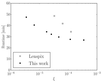
Appendix A Simulated CMB sky and Lenspix modifications

To simulate lensed CMB data we modify publicly available code Lenspix Lewis (2005). In this code the unlensed CMB is first evaluated on a high resolution equicylindrical grid. The lensed CMB is then evaluated on a lower resolution Healpix grid Gorski et al. (1999) through a remapping by a deflection field, determined by a gradient of the lensing potential $\phi$. Values of the unlensed CMB at points which are remapped onto the Healpix grid points are obtained using a bi-cubic interpolation from the high resolution grid. Our simulations are run with precision parameters nside = 4096 and lmax = 8000.

The precision with which the code calculates the lensed power spectra depends on the point density of the high resolution grid, which is parameterized by an oversampling factor interp_factor. Simulations with interp_factor $\sim$ 2, which were the largest we could originally run on a single node of our computer cluster due to limited memory, lead to lensed CMB power spectra biased at high $\ell$. Such bias leads to $\sim 0.2$ standard deviations shift in the likelihood function in the $\ln A_{s}$ direction (with other cosmological parameters fixed); we did not investigate other parameters in depth but in general parameters constrained by high $\ell$ data are sensitive to this bias.

This power spectra bias can be quantified by a parameter

$$\xi=\frac{C^{TT}_{3000}\Big{|}_{\phi=0}-\tilde{C}^{TT}_{3000}}{\tilde{C}^{TT}_{3000}},$$ (27)

relative difference at $\ell=3000$ of the temperature power spectrum $C^{TT}$ “lensed” in Lenspix by a zero-deflection field and the unlensed temperature power spectrum $\tilde{C}^{TT}$. If interpolation was exact $\xi$ would vanish. However, the unlensed and lensed CMB are evaluated at different grids and interpolation leads to numerical bias even when there is no lensing present. This bias appears to be – up to cosmic variance – independent of the cosmology and comparable in temperature and polarization. It typically grows with investigated multipole, for comparison we therefore choose the largest data multipole considered in the paper, $\ell=3000$.

To overcome the large $\xi$ bias and avoid the related shifts in the likelihood function, we modify the code such that it works only with smaller portions of the high resolution map of unlensed CMB at any given time and never stores the whole map in memory. This allows us to run with higher values of interp_factor and achieve smaller values of $\xi$.

We further replace the original high precision calculation of partial derivatives of the unlensed CMB variables, which is part of the Lenspix interpolation algorithm, by a less precise (for a given high resolution grid) but significantly faster routine. This enables us to obtain higher interpolation precision without sacrificing runtime by increasing the density of the high resolution grid of the unlensed CMB.

Finally, the precision of variables describing the angular positions of the points in the high resolution grid is increased to avoid certain artifacts in lensed CMB maps.

We compare values of $\xi$ and runtime for several values of interp_factor with the original and simplified calculation of the partial derivatives in Fig. 20. It is clear that although the original routine is superior for a fixed high resolution grid, for a fixed runtime it is advantageous to use a simpler partial derivative calculation and increase the density of the grid. Simulations used in this work were calculated with interp_factor = 4.

Figure 21: Lensed power spectra bias $b_{\ell}^{XY}$ for several values of $\ell$, averaged over 2000 lensed CMB simulations calculated with the precision settings used in this work (black). In red the same quantities determined from 400 lensed CMB simulations calculated with original Lenspix interpolation algorithm with interp_factor— = 2. Error bars represent errors on the mean estimated from the simulated values.

Figure 22: Lensed $C_{\ell}^{BB}$ calculated with lensing potential increased by $\Delta C^{\phi\phi}_{\ell}$ which corresponds to parameter shifts listed in Tab. 2 and its representation in terms of the first $N\in{0\ldots 4}$ PCs (top: absolute; bottom percent error between the two).

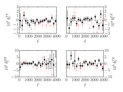
To judge agreement between the lensed power spectra from simulations and the theoretical expectation calculated by CAMB, we define bias variables

$$b^{XY}_{\ell}=\frac{\sum_{\ell^{\prime}}\ell^{\prime}(\ell^{\prime}+1)\Delta C_{\ell^{\prime}}^{XY}}{\sum_{\ell^{\prime}}\ell^{\prime}(\ell^{\prime}+1)C_{\ell^{\prime}}^{XY,\mathrm{fid}}},$$ (28)

which can be evaluated for each simulated CMB sky. Here the sums go over a bin of width $\Delta\ell=200$ centered on $\ell$ and $\Delta C_{\ell^{\prime}}^{XY}$ is a difference between simulated and expected value of power spectra, defined in (9). In Fig. 21 we plot average values of $b^{XY}_{\ell}$ from simulations for several values of $\ell$; we show the levels of bias achieved with both the simulations settings used in this work and the original Lenspix code with interp_fact = 2. In the latter, a small bias is visible for $XY=TT,EE$.

Appendix B Sky Coverage and Optical Depth

A ground-based CMB Stage 4 experiment is unlikely to usefully measure CMB temperature and polarization on the full sky. For that reason, in this Appendix we use a Fisher analysis to reexamine some of the results of §III for an experiment which observes 40% of the sky and measures temperature and polarization power spectra in the multipole range $\ell=30-3000$. We additionally neglect covariance induced by the sky mask by simply scaling the full sky covariance with the sky fraction. Information from the largest scales is represented by adding a Planck-like prior on $\tau$, corresponding to a standard deviation of $\sigma_{\tau}=0.01$.

As is to be expected, absence of the large scale measurements significantly degrades the absolute constraints on cosmological parameters. However, the relative effects of the non-Gaussian covariance do not become significantly more important. For example, degradation of the most affected parameter combination, as expressed through the ratio $\sigma_{M}^{\mathrm{ng}}/\sigma_{M}^{\mathrm{g}}$ in $\Lambda$CDM and analogous ratios for the other cosmological models, increases by less than 4% when omitting information from $\ell<30$. The largest effect of this omission is in the $\tau-A_{s}$ plane. When large angle polarization data are improved over Planck, they further break the $A_{s}e^{-2\tau}$ degeneracy in the heights of the acoustic peaks. Without this improvement, lensing measurements become more competitive in breaking this degeneracy and consequently constraints on these two parameters are degraded by $\sim 10\%$ in all three cosmological models investigated in §III.

Figure 23: Dependence of $\chi^{2}_{\mathrm{PC},N}$ (30), measure of error caused by approximating the lensing potential using first $N$ principal component, on $N$. In this case $\Delta C_{\ell}^{\phi\phi}$ corresponds to parameter shifts listed in Tab. 2.

Appendix C Number of lensing principal components

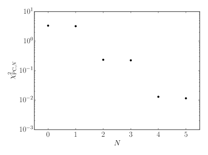
Two considerations guide the choice of the number of principal components of the lensing potential to be measured from the lensed CMB power spectra. Keeping a larger number of PCs leads to a more accurate description of the lensed power spectra. On the other hand, increasing number of parameters slows down convergence of the MCMC calculations, requiring physicality priors, since the higher PCs are more poorly constrained by definition. In this section we justify our choice of using five PCs.

First we look at the fidelity in reproducing lensing effects in the observed $C^{XY}_{\ell}$ power spectra. For definiteness, we perturb the fiducial $C^{\phi\phi}_{\ell}$ by a $\Delta C^{\phi\phi}_{\ell}$ which corresponds to shifts in the cosmological parameters given in Table 2 (at fixed unlensed power spectra). This change represents a realistic change in the lensing potential which might be encountered in a real analysis, as cosmological model with parameters from Tab. 2 is between 68% and 95% probability contours for $\Lambda$CDM+$w$ model in the simulation investigated in the main text. For completeness and comparison to the results in the main text, the lensing principal components arising from this change are

$$\Theta^{(i)}=\{-0.012,0.11,-0.011,-0.06,-0.012\}.$$ (29)

Note that the investigated parameter change is not aligned with change of $M^{w}$ from (29), nor need it be since it represents the degeneracy direction rather than the direction most affected by lens covariance.

Table 2: Shifts in the cosmological parameters used to probe approximations of the lensing potential in terms of lensing PCs

Parameter	Shift
$h$	0.175
$\Omega_{c}h^{2}$	$-1.0\times 10^{-3}$
$\Omega_{b}h^{2}$	$3.5\times 10^{-5}$
$n_{s}$	$1.2\times 10^{-3}$
$A_{s}$	$-1.6\times 10^{-11}$
$\tau$	$-2.2\times 10^{-3}$
$w$	$-0.52$

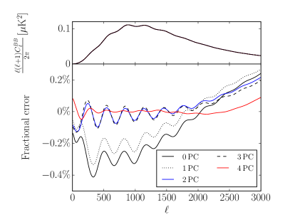
In top panel of Fig. 22 we show the resulting $C^{BB}_{\ell}$ power spectrum calculated with lensing potential changed by the full $\Delta C^{\phi\phi}_{\ell}$ vs. when this change is approximated using the first $N\in\{0,1,2,3,4\}$ lensing PCs; the difference is too small to be visible directly and so the bottom panel shows the percent error. Note that the smallness of these changes explains why in the main text approximations based on linearizing power spectra deviations and PC amplitudes are excellent even for relatively large cosmological parameter shifts.

Since the change in Eq. 29 is dominated by $\Theta^{(2)}$, most of the improvement in fidelity comes when adding that component. In fact for this particular $\Delta C^{\phi\phi}_{\ell}$, first two PCs are sufficient to faithfully describe effects of lensing in $TT$, $EE$ and $TE$ power spectra extremely well. The next large jump in fidelity comes with the fourth PC which is associated with the high multipole range of $BB$ in Fig. 22. We checked several other choices of allowed $\Delta C^{{\phi\phi}}_{\ell}$ and for all of them four principal components lead to small errors on the power spectra level.

To quantify the total significance of the errors we construct

$$\chi^{2}_{\mathrm{PC},N}=\sum_{\begin{subarray}{c}\text{$i,j$}\end{subarray}}\delta D_{i}(N)\left(\mathrm{Cov}_{i,j}\right)^{-1}\delta D_{j}(N),$$ (30)

where for brevity we introduce $\delta D_{i}(N)=\delta C_{\ell}^{XY}(N)$, the power spectrum error caused by approximating $\Delta C^{\phi\phi}_{\ell}$ using the first $N$ PCs, with $i$ indexing all multipoles and power spectra types. As $N$ increases, the PCs approximate the full effect of lensing better and $\chi^{2}_{\mathrm{PC},N}$ decreases. In Fig. 23 we show this dependence; as we saw before, adding fourth PC leads to a significant improvement in our ability to capture the effects of gravitational lensing on the CMB. For some choices of $\Delta C^{\phi\phi}_{\ell}$, adding fifth PC improves $\chi^{2}_{\mathrm{PC},N}$ by a factor of a few on top of the $\sim$ hundred-fold improvement in $\chi^{2}_{\mathrm{PC},N}$ arising from using four PCs. For this work we decided to include fifth PC into the analysis as well, even though its inclusion is not expected to have any significant impact on the results.

References

- Ade et al. (2016a) P. A. R. Ade et al. (Planck), Astron. Astrophys. 594, A13 (2016a), arXiv:1502.01589 [astro-ph.CO] .
- Hu (2001) W. Hu, Phys. Rev. D64, 083005 (2001), arXiv:astro-ph/0105117 [astro-ph] .
- Smith et al. (2007) K. M. Smith, O. Zahn, and O. Dore, Phys. Rev. D76, 043510 (2007), arXiv:0705.3980 [astro-ph] .
- Lewis and Challinor (2006) A. Lewis and A. Challinor, Phys. Rept. 429, 1 (2006), arXiv:astro-ph/0601594 [astro-ph] .
- Hirata et al. (2008) C. M. Hirata, S. Ho, N. Padmanabhan, U. Seljak, and N. A. Bahcall, Phys. Rev. D78, 043520 (2008), arXiv:0801.0644 [astro-ph] .
- Hanson et al. (2013) D. Hanson et al. (SPTpol), Phys. Rev. Lett. 111, 141301 (2013), arXiv:1307.5830 [astro-ph.CO] .
- Das et al. (2011) S. Das et al., Phys. Rev. Lett. 107, 021301 (2011), arXiv:1103.2124 [astro-ph.CO] .
- Keisler et al. (2011) R. Keisler et al., Astrophys. J. 743, 28 (2011), arXiv:1105.3182 [astro-ph.CO] .
- Ade et al. (2014) P. A. R. Ade et al. (Planck), Astron. Astrophys. 571, A17 (2014), arXiv:1303.5077 [astro-ph.CO] .
- Keisler et al. (2015) R. Keisler et al. (SPT), Astrophys. J. 807, 151 (2015), arXiv:1503.02315 [astro-ph.CO] .
- Ade et al. (2016b) P. A. R. Ade et al. (Planck), Astron. Astrophys. 594, A15 (2016b), arXiv:1502.01591 [astro-ph.CO] .
- Ade et al. (2016c) P. A. R. Ade et al. (BICEP2, Keck Array), (2016c), arXiv:1606.01968 [astro-ph.CO] .
- Sherwin et al. (2017) B. D. Sherwin et al., Phys. Rev. D95, 123529 (2017), arXiv:1611.09753 [astro-ph.CO] .
- Benson et al. (2014) B. A. Benson et al. (SPT-3G), Proceedings, SPIE Astronomical Telescopes + Instrumentation 2014: Millimeter, Submillimeter, and Far-Infrared Detectors and Instrumentation for Astronomy VII: Montreal, Quebec, Canada, June 24-27, 2014, Proc. SPIE Int. Soc. Opt. Eng. 9153, 91531P (2014), arXiv:1407.2973 [astro-ph.IM] .
- Henderson et al. (2016) S. W. Henderson et al., Proceedings, 16th International Workshop on Low Temperature Detectors (LTD 16): Grenoble, France, July 20-24, 2015, J. Low. Temp. Phys. 184, 772 (2016), arXiv:1510.02809 [astro-ph.IM] .
- Wu et al. (2016) W. L. K. Wu et al., Proceedings, 16th International Workshop on Low Temperature Detectors (LTD 16): Grenoble, France, July 20-24, 2015, J. Low. Temp. Phys. 184, 765 (2016), arXiv:1601.00125 [astro-ph.IM] .
- Abazajian et al. (2016) K. N. Abazajian et al. (CMB-S4), (2016), arXiv:1610.02743 [astro-ph.CO] .
- Motloch et al. (2017) P. Motloch, W. Hu, and A. Benoit-Lévy, Phys. Rev. D95, 043518 (2017), arXiv:1612.05637 [astro-ph.CO] .
- Smith et al. (2006) K. M. Smith, W. Hu, and M. Kaplinghat, Phys. Rev. D74, 123002 (2006), arXiv:astro-ph/0607315 [astro-ph] .
- Benoit-Levy et al. (2012) A. Benoit-Levy, K. M. Smith, and W. Hu, Phys. Rev. D86, 123008 (2012), arXiv:1205.0474 [astro-ph.CO] .
- Green et al. (2016) D. Green, J. Meyers, and A. van Engelen, (2016), arXiv:1609.08143 [astro-ph.CO] .
- Peloton et al. (2016) J. Peloton, M. Schmittfull, A. Lewis, J. Carron, and O. Zahn, (2016), arXiv:1611.01446 [astro-ph.CO] .
- Knox (1995) L. Knox, Phys. Rev. D 52, 4307 (1995), astro-ph/9504054 .
- Lewis et al. (2000) A. Lewis, A. Challinor, and A. Lasenby, Astrophys. J. 538, 473 (2000), arXiv:astro-ph/9911177 [astro-ph] .
- Lewis (2005) A. Lewis, Phys. Rev. D71, 083008 (2005), arXiv:astro-ph/0502469 [astro-ph] .
- Lewis and Bridle (2002) A. Lewis and S. Bridle, Phys. Rev. D66, 103511 (2002), arXiv:astro-ph/0205436 [astro-ph] .
- Gelman and Rubin (1992) A. Gelman and D. B. Rubin, Statist. Sci. 7, 457 (1992).
- Gorski et al. (1999) K. M. Gorski, B. D. Wandelt, F. K. Hansen, E. Hivon, and A. J. Banday, (1999), arXiv:astro-ph/9905275 [astro-ph] .