Quantum chaos for nonstandard symmetry classes in the Feingold-Peres model of coupled tops

Abstract

We consider two coupled quantum tops with angular momentum vectors $\mathbf{L}$ and $\mathbf{M}$. The coupling Hamiltonian defines the Feingold-Peres model, which is a known paradigm of quantum chaos. We show that this model has a nonstandard symmetry with respect to the Altland-Zirnbauer tenfold symmetry classification of quantum systems, which extends the well-known threefold way of Wigner and Dyson (referred to as ‘standard’ symmetry classes here). We identify the nonstandard symmetry classes BD$I_{0}$ (chiral orthogonal class with no zero modes), BD$I_{1}$ (chiral orthogonal class with one zero mode), and C$I$ (antichiral orthogonal class) as well as the standard symmetry class A$I$ (orthogonal class).
We numerically analyze the specific spectral quantum signatures of chaos related to the nonstandard symmetries. In the microscopic density of states and in the distribution of the lowest positive energy eigenvalue we show that the Feingold-Peres model follows the predictions of the Gaussian ensembles of random-matrix theory in the appropriate symmetry class if the corresponding classical dynamics is chaotic. In a crossover to mixed and near-integrable classical dynamics we show that these signatures disappear or strongly change.

I Introduction

We consider two coupled quantum tops with respective angular momentum operators $\mathbf{L}=(L_{x},L_{y},L_{z})^{T}$ and $\mathbf{M}=(M_{x},M_{y},M_{z})^{T}$ and Hamiltonian

$$H=\frac{1+\lambda}{j+1/2}\left(L_{z}+M_{z}\right)+\frac{4(1-\lambda)}{(j+1/2)^{2}}L_{x}M_{x}$$ (1)

where $\lambda\in[0,1]$ is a parameter that changes the relative strength of the two parts, and $j$ is the (half-integer or integer) total angular momentum quantum number of both tops. More than 30 years ago Feingold and Peres introduced this as a paradigmatic model for quantum chaos fp ; fmp . We now reconsider this model in the light of its nonstandard symmetry properties in the tenfold symmetry classification of quantum systems by Altland and Zirnbauer AZ1 ; AZ2 ; Zirni . When Feingold and Peres used this model only the three standard symmetry classes of Wigner and Dyson Wigner1 ; Wigner2 ; Dyson1 ; Dyson2 had been known for quantum systems. The first nonstandard symmetry classes that have been discovered by Verbaarschot and Zahed Ver1 ; Ver2 are the three chiral symmetry classes (see also gade ; slevin ). Altland and Zirnbauer then found the remaining four symmetry classes and revealed a direct connection between the mathematical structure behind this classification of quantum systems and Cartan’s tenfold classification of symmetric spaces Zirni . In random-matrix theory some of the relevant ensembles had already been known without awareness of their application to quantum systems (e.g. the ensembles that go back to Wishart wishart ). The presence of a nonstandard symmetry in the Feingold-Peres model defined by Eq. (1) and its implication for universal spectral properties have thus remained undetected at the time. Our aim is to reintroduce the model as a paradigm to understand the quantum signatures of chaos related to nonstandard symmetries and numerically analyze how these signatures change in a crossover between chaotic and integrable motion.
The common feature of the seven nonstandard symmetry classes is the presence of a mirror symmetry in the energy eigenvalue spectrum around a specific energy $E_{F}$: if $E_{F}+E$ is an eigenvalue, so is $E_{F}-E$ and they have the same degeneracy. Physically this is typically realized in fermionic many-body systems such as the quasiparticle excitations in superconductors and superfluids described by the Bogoliubov-de Gennes equation or relativistic Fermions described by the Dirac equation. In these cases $E_{F}$ is the Fermi energy and all energy eigenstates with energies below $E_{F}$ are occupied in the ground state. In the following we will set $E_{F}=0$ without loss of generality. The spectral mirror symmetry alters universal spectral properties such as level-repulsion near the symmetry energy $E=0$ and the effects die off quickly on the scale of the mean level spacing. Far away from the symmetry point the standard behavior of the three Wigner-Dyson symmetry classes is recovered. The nonstandard symmetry classes are well studied in random-matrix theory and physically more realistic disordered systems such disordered superconductors AZ1 ; AZ2 or Dirac particles in a disordered gauge field Ver1 ; Ver2 . The Feingold-Peres model is an example of a quantum system where the nonstandard symmetry classes are realized in a finite Hilbert space. In such a setting one may describe the nonstandard symmetry classes in terms of anticommuting operators: the spectral mirror symmetries may be described in terms of unitary (chirality) or antiunitary (charge-conjugation) operators $C$ such that $HC+CH=0$, or $CHC^{-1}=-H$. It is sufficient to consider $C^{2}=\pm 1$. Considering all possible (nonredundant) combinations of the various types (or nonexistence) of operators $C$ with the threefold classification with respect to the behavior under time-reversal transformations leads to the tenfold classification, see stargraphI .
For the Feingold-Peres model the operator $C$ may be identified as a unitary operator of the form

$$C=e^{i\alpha}\mathcal{R}^{(1)}_{x}(\pi)\otimes\mathcal{R}^{(2)}_{y}(\pi)=e^{i\alpha-i\pi L_{x}-i\pi M_{y}}$$ (2)

where $e^{i\alpha}$ is a phase factor that has no effect in the present discussion but will need to be included later. This describes a rotation of the first top by an angle $\pi$ around the x-axis and a rotation of the second top by the same angle about the y-axis. As a transformation this changes the sign of all angular momentum components that are not aligned with the axis of rotation. In particular one has $CL_{z}C^{-1}=-L_{z}$, $CM_{z}C^{-1}=-M_{z}$, $CL_{x}C^{-1}=L_{x}$ (no sign change here), and $CM_{x}C^{-1}=-M_{x}$. Altogether one then has

$$CHC^{-1}=-H$$ (3)

which implies nonstandard symmetries. As the Hamiltonian is also invariant under two unitary symmetries (exchange of the two tops $\mathbf{M}\leftrightarrow\mathbf{L}$ and rotations of both tops by $\pi$ around the $z$ axis) the detailed classification needs to be done carefully, considering each invariant subspace separately. In Section III we will show that different invariant subspaces realize different symmetry classes and that the classification also depends on whether $j$ is integer or half-integer. We will also show there that the Hamiltonian has a generalized time-reversal symmetry.

In random-matrix theory statistical correlations in the eigenvalue spectra for all symmetry classes have been studied with great detail using Gaussian ensembles. This is a powerful tool for disordered systems and quantum chaos as the nontrivial predictions of the Gaussian ensembles are known to be universal (with varying degree of rigor depending on the setting). Being deliberately vague the corresponding universality classes comprise quantum systems with ‘sufficient complexity’. Universal statistics of spectral fluctuations means that appropriately averaged spectral functions in physical systems are independent of the details of the system and only depend on the symmetry classification if measured on the right energy scale. The latter turns out to be the mean level spacing. Characterizing the universality classes in detail (specifying what ‘sufficient complexity’ means) and finding clear criteria whether a given system should be universal or not is usually a very hard problem if one pursues rigor. Numerical analysis on the other hand gives abundant evidence and examples for universal spectral statistics. In general terms universality can be achieved either by an appropriate amount of disorder in the system or by the presence of chaos in the corresponding classical dynamics, i.e. by the presence of quantum chaos.

In this paper we follow the quantum chaos approach to universal spectral statistics. This approach is well established for the three standard Wigner-Dyson symmetry classes. In 1983 Bohigas, Giannoni and Schmit (BGS) BGS conjectured that the spectral statistics (on the scale of the mean level spacings) of individual quantum chaotic systems is universal with three universality classes corresponding to the three Gaussian Wigner-Dyson ensembles of random-matrix theory (GOE, GUE, and GSE). This conjecture was first confirmed numerically and was a major challenge in quantum chaos for more than 20 years diagonal ; actioncorrelation ; SieberRichter before complete microscopic derivations using semiclassical approaches appeared: first for quantum graph models (a quantum particle that moves freely on a network described by a metric graph) GA1 ; GA2 (see also quantumgraphs as a review for quantum chaos on graphs) and then for ‘generic’ quantum chaotic systems Essen (see SuSyreview and references therein for a review). Hopes for a rigorous and general proof had to be abandoned due to the existence of ‘ungeneric’ counter examples catmaps ; arithmetic . Still, one may hope for rigorous proofs for certain well-defined quantum models (e.g. quantum graphs).
The BGS conjecture may directly be extended to nonstandard symmetry classes (see Section IV.1) where the quantum chaos approach has so far been restricted to quantum graph models stargraphI ; stargraphII and to Andreev billiards MagneticAndreev . The nonstandard symmetries have a direct and universal impact on the (microscopic) density of states near $E=0$. For both, quantum graphs and quantum chaotic magnetic Andreev billiards a periodic-orbit analysis (the self-dual approximation) based on Gutzwiller-type semiclassical trace formulas is consistent with the generalized BGS conjecture. As is well known kosztin nonmagnetic Andreev billiards cannot show proper quantum chaos (in the sense that the corresponding classical dynamics is fully chaotic) and they do not belong in the universality class of the Gaussian ensembles for the appropriate symmetry class. They show, however, very interesting behavior in their own right and may be described in terms of more restricted Gaussian ensembles (see AndreevReview and references therein). For quantum graphs all ten symmetry classes may be realized and they give numerical evidence that supports the generalized BGS conjecture stargraphII .
We will show that the Feingold-Peres model is a further model where some nonstandard symmetry classes are realized and that it can be used to study the corresponding universal signatures in the statistics of eigenvalues. More general models based on coupling two tops may be used as paradigmatic systems to study universal quantum signatures of chaos related to all nonstandard symmetry classes.

Let us now give an overview of the paper. In Section II we introduce the Feingold-Peres model together with its corresponding classical dynamics and summarize the known crossover from chaotic to integrable dynamics using additional numerical simulations. In Section III we analyze the proper symmetry classification of this model and establish that different subspectra with respect to the remaining unitary symmetries may lie in different symmetry classes. In Section IV we then establish numerically that the quantum spectra are consistent with the predictions of the random-matrix ensembles of the corresponding symmetry class and thus with the generalized BGS conjecture. This is obtained without any average over disorder by averaging over different representations defined by the angular momentum quantum number $j$ or, equivalently different values of the effective Planck constant $\hbar=1/(j+1/2)$. Section V summarizes the main conclusions and gives an outlook on future directions.

II The Feingold-Peres model and its corresponding classical dynamics

Let us quickly summarize the theoretical setting for the Hamiltonian (1) of the Feingold-Peres model. The fundamental quantum observables are described by the components of angular momentum operators. They satisfy the standard commutation relations

$$\left[L_{k},L_{l}\right]=i\sum_{m\in\{x,y,z\}}\epsilon_{klm}L_{m},\quad\left[M_{k},M_{l}\right]=i\sum_{m\in\{x,y,z\}}\epsilon_{klm}M_{m},\quad\text{and}\quad\left[L_{k},M_{l}\right]=0$$ (4)

where $k,l\in\{x,y,z\}$ and $\epsilon_{klm}$ is the totally antisymmetric Levi-Civita tensor with $\epsilon_{xyz}=1$. They generate the group $SU(2)\times SU(2)$ and we assume that the Hilbert space $V$ is an irreducible representation of this group such that both angular momenta have the same total angular momentum $\mathbf{L}^{2}=\mathbf{M}^{2}=j(j+1)$ and the dimension is $N=\mathrm{dim}\ V=(2j+1)^{2}$. The standard basis will be denoted by $\{|m_{1},m_{2}\rangle\}$ with $m_{1},m_{2}\in\{-j,-j+1,\dots,j\}\equiv Z_{j}$. It consists of common eigenstates to the $z$-components of both angular momenta $L_{z}|m_{1},m_{2}\rangle=m_{1}|m_{1},m_{2}\rangle$ and $M_{z}|m_{1},m_{2}\rangle=m_{2}|m_{1},m_{2}\rangle$ .

II.1 Classical dynamics of two coupled tops

The classical limit of the Feingold-Peres model is well understood. In their original work Feingold and Peres fp observed a crossover from chaotic to regular dynamics at energy $E=0$ as the system parameter $\lambda$ increases from zero to one. In this section we summarize the main results and add an up-to-date numerical analysis of the crossover for comparison with our analysis of the quantum signatures of this crossover at the relevant system parameters.

The corresponding classical dynamics of the Feingold-Peres model is obtained by replacing the rescaled quantum angular momentum operators $L_{k}/(j+1/2)$ and $M_{k}/(j+1/2)$ ($k=x,y,z$) with commutator relations (4) by classical angular momentum variables $\mathcal{L}_{k}$ and $\mathcal{M}_{k}$ such that $\mathcal{L}_{x}^{2}+\mathcal{L}_{y}^{2}+\mathcal{L}_{z}^{2}=\mathcal{M}_{x}^{2}+\mathcal{M}_{y}^{2}+\mathcal{M}_{z}^{2}=1$. The classical angular momentum variables thus span a phase space $S^{2}\times S^{2}$, the Cartesian product of two spheres. On this phase space they obey the standard angular momentum Poisson bracket relations

$$\left\{\mathcal{L}_{k},\mathcal{L}_{l}\right\}=-\sum_{m\in\{x,y,z\}}\epsilon_{klm}\mathcal{L}_{m},\quad\left\{\mathcal{M}_{k},\mathcal{M}_{l}\right\}=-\sum_{m\in\{x,y,z\}}\epsilon_{klm}\mathcal{M}_{m},\quad\text{and}\quad\left\{\mathcal{L}_{k},\mathcal{M}_{l}\right\}=0\ .$$ (5)

The classical dynamics is most easily obtained by performing the corresponding substitutions in the quantum Heisenberg equations which leads Hamiltonian equations according to

$$\frac{d}{dt}L_{k}=i(j+1/2)\left[H,L_{k}\right]\quad\mapsto\quad\frac{d}{dt}\mathcal{L}_{k}=\left\{\mathcal{H},\mathcal{L}_{k}\right\}$$ (6)

and, analogously for $M_{k}\to\mathcal{M}_{k}$. The Hamilton function for the Feingold-Peres model is

$$\mathcal{H}=\left(1+\lambda\right)\left(\mathcal{L}_{z}+\mathcal{M}_{z}\right)+4(1-\lambda)\mathcal{L}_{x}\mathcal{M}_{x}\ .$$ (7)

We have used units such that $\hbar=1/(j+1/2)$ which links the classical limit $\hbar\to 0$ to the limit $j\to\infty$. It also sends the Hilbert space dimension to infinity $N\to\infty$. The classical limit can be constructed explicitly if one assumes that the state of the system is in a generalized $SU(2)\times SU(2)$ coherent state and takes the expectation value of both sides of the quantum Heisenberg equations. Identifying $\mathcal{L}_{k}=\frac{1}{(j+1/2)}\langle L_{k}\rangle$, $\mathcal{M}_{k}=\frac{1}{(j+1/2)}\langle M_{k}\rangle$ and taking the limit $j\to\infty$ then results in the classical equations of motion. Needless to say the appearance of factors $j+1/2$ accompanying each angular momentum operator is essential for this limit to work. Note however, that replacing $j+1/2$ by just $j$ (and thus $\hbar=1/j$) leads to the same limit – we write $j+1/2$ merely because this is the more natural expansion in the semiclassical regime.
As the product of two spheres the classical phase space has dimension four. There are many ways to introduce two pairs of canonical coordinates $(P_{1},Q_{1},P_{2},Q_{2})$ with canonical Poisson brackets $\{P_{\ell},Q_{\ell^{\prime}}\}=\delta_{\ell\ell^{\prime}}$ and $\{P_{\ell},P_{\ell^{\prime}}\}=\{Q_{\ell},Q_{\ell^{\prime}}\}=0$ on this phase space. While any choice necessarily leads to some coordinate singularity we found the choice

$$\mathcal{L}_{x}= \sqrt{1-P_{1}^{2}}\cos Q_{1}, \mathcal{M}_{x}= \sqrt{1-P_{2}^{2}}\cos Q_{2},$$ (8a)

$$\mathcal{L}_{y}= \sqrt{1-P_{1}^{2}}\sin Q_{1}, \mathcal{M}_{y}= \sqrt{1-P_{2}^{2}}\sin Q_{2},$$ (8b)

$$\mathcal{L}_{z}= P_{1}, \mathcal{M}_{z}= P_{2}$$ (8c)

most convenient.

For $\lambda=1$ the classical dynamics is clearly integrable with two constants of motion $\mathcal{L}_{z}$ and $\mathcal{M}_{z}$. Peres and Feingold have shown that, as $\lambda$ is decreased, there is a crossover to mixed and chaotic dynamics on the energy shell $\mathcal{H}\equiv E=0$ for intermediate values and chaos being maximally developed at $\lambda=0$. In the remainder of this section we summarize the relevant findings using our own numerical calculations.
The transition can most easily be seen with Poincaré plots as shown in Fig. 1. These were obtained by numerically integrating the classical equations of motion with initial conditions that satisfy $\mathcal{H}(P_{1},Q_{1},P_{2},Q_{2})=0$ and $Q_{2}=\frac{\pi}{2}$. The latter condition defines our choice for the Poincaré surface of section. Whenever the trajectory crosses the Poincaré surface we record the coordinates $Q_{1}\in[0,2\pi)$ and $P_{1}\in[-1,1]$ that describe the orientation of the first top. The symmetries of the dynamics allow us to reduce this Poincaré map to $Q_{1}\in[0,\pi)$ and $P_{1}\in[-1,1]$ which is shown in Fig. 1. The remaining mirror symmetry about $Q_{1}=\pi/2$ of Poincaré plots is related to the time-reversal symmetry of the dynamics.

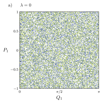
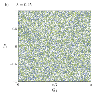
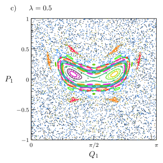
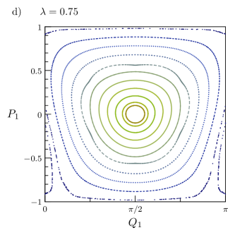
Figure 1: (Color online) Poincaré plots in the energy shell $E=0$ for various values of the coupling parameter $\lambda$. For $\lambda=0$ (graph a)) and $\lambda=0.25$ (graph b)) the Poincaré plots show no structures indicating that the dynamics is dominantly chaotic. While very small regular islands cannot be excluded they would have to be on scales much smaller than the resolution of this plot. At $\lambda=0.5$ (graph c)) the plot shows a typical mixed phase space with a large chaotic region and a regular island. At $\lambda=0.75$ (graph d)) the plot shows a near integrable dynamics.

We do not show any plots for $0.75<\lambda<1$ as the graph only changes slightly. In the limit $\lambda\to 1$ the lines follow the level curves of $\mathcal{L}_{y}=\sqrt{1-P_{1}^{2}}\sin Q_{1}$ and this is already visible clearly at $\lambda=0.75$. At first sight one may expect to see the level lines of $P_{1}$ as the Hamiltonian at $\lambda=1$ reduces to $\mathcal{H}=2(P_{1}+P_{2})$ which has obvious constants of motion $P_{1}$ and $P_{2}$. While this is true the dynamics is indeed highly degenerate as both tops rotate at the same frequency with constant $z$-components of their angular momentum vectors. This implies that the Poincaré map maps each point $(Q_{1},P_{1})$ back to itself and that each trajectory in the energy shell $E=0$ is a periodic orbit with same period. In such a situation the perturbation that sets in for $\lambda<1$ defines the invariant tori visible in a Poincaré map and a simple perturbative calculation shows that the Poincaré map follows level lines of $\mathcal{L}_{y}$.

While the Poincaré plots give a clear qualitative picture of the crossover from chaotic to integrable motion let us also give a more quantitative analysis of the degree of chaos by considering the exponential dependency on initial conditions as measured by the Lyapunov exponents. For this we numerically calculate

$$\Lambda_{\epsilon}(t)=\frac{1}{t}\log\frac{\Delta_{\epsilon}(t)}{\epsilon}$$ (9)

where $\Delta_{\epsilon}(t)=\sqrt{\Delta{P_{1}}^{2}+\Delta{Q_{1}}^{2}+\Delta{P_{2}}^{2}+\Delta{Q_{2}}^{2}}$ is the distance between two trajectories with initial distance $\Delta_{\epsilon}(0)=\epsilon>0$. The Lyapunov exponent is obtained in the limit $\Lambda=\lim_{t\to\infty}\lim_{\epsilon\to 0}\Lambda_{\epsilon}(t)$ (where the order of the two limits is important). Numerically one has to work with a finite but small value for $\epsilon$ (in our case $\epsilon\approx 10^{-12}$). For any finite value of $\epsilon$ one always has $\Lambda_{\epsilon}(t)\to 0$ as $t\to\infty$ and to estimate the Lyapunov exponent one has to use a cutoff time $t_{c}$ that ensures that the deviation $\Delta_{\epsilon}(t_{c})$ is still small compared to the extension of phase space.

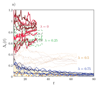
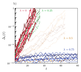
Figure 2: (Color online) Exponential dependence on initial conditions as measured by $\Lambda_{\epsilon}(t)$ (left graph a)) and $\Delta_{\epsilon}(t)$ (logarithmic plot in right graph b)). These are shown for ten trajectories for each of the values $\lambda=0$ (fat red lines), $\lambda=0.25$ (dashed green lines), $\lambda=0.5$ (dotted yellow lines), and $\lambda=0.75$ (thin blue lines). For $\lambda=0.5$ 9 trajectories are in the chaotic region (thin dotted lines) and one is inside the regular island (fat dotted line). Cutoff times were chosen such that most trajectories for the same value $\lambda$ obey $\Delta_{\epsilon}(T_{c})\ll 1$.
The shaded region on the left graph for $\Lambda_{\epsilon}(t)$ is bounded by $\frac{\log t}{t}$ which gives the typical decay of $\Lambda_{\epsilon}(t)$ when the Lyapunov exponent vanishes.

In Fig. 2 we show plots for $\Lambda_{\epsilon}(t)$ and $\Delta_{\epsilon}(t)$ for a number of trajectories for different values of the coupling parameter $\lambda$. The findings are consistent with the Poincaré plots in Fig. 1. For $\lambda=0$ we find chaotic dynamics as can clearly be seen in the exponential increase of $\Delta_{\epsilon}(t)$. Though the Lyapunov exponents have not yet converged one may give an estimate $0.65<\Lambda<1$. For $\lambda=0.25$ the dynamics is also chaotic but the exponential increase is a bit weaker $0.55<\Lambda<0.85$. For $\lambda=0.5$ the mixed phase space shows up in that some trajectories show exponential dependency on initial conditions with $0.2<\Lambda<0.4$ while others do not show this and the numerics is consistent with $\Lambda=0$. For the ten plotted trajectories initial conditions were chosen random and nine turned out to be chaotic and one regular. We have checked consistency with the corresponding Poincaré plot.
It is certainly possible to improve these numerical results with some effort. For our purpose, which is to investigate quantum signatures of chaos in the spectral fluctuations close to $E=0$ we have given a sufficient summary of the corresponding classical dynamics.

III Reduction to invariant subspaces and symmetry classification

Let us now come back to the quantum dynamics and reduce the system using all available unitary symmetries before considering the symmetry classification of the Hamiltonian in the reduced subspaces of the Hilbert space $V$ according to the Altland-Zirnbauer tenfold way.

III.1 Unitary symmetries and their invariant subspaces

The Hamiltonian (1) is invariant under exchange of the two tops and under a simultaneous rotation of both tops by an angle $\pi$ around the $z$-axis. Let us denote the corresponding unitary quantum operators by $U_{1}$ and $U_{2}$ and define them through their action in the standard basis

$$U_{1}|m_{1},m_{2}\rangle= |m_{2},m_{1}\rangle$$ (10a)

$$U_{2}|m_{1},m_{2}\rangle= e^{i\pi(2j-m_{1}-m_{2})}|m_{1},m_{2}\rangle$$ (10b)

for $m_{1},m_{2}\in Z_{j}$. So $U_{1}$ describes the exchange of tops. It has eigenvectors $|m_{1},m_{2}\rangle\pm|m_{2},m_{1}\rangle$ with eigenvalues $\pm 1$ and thus obeys $U_{1}^{2}=1$. It acts on angular momentum operators as $U_{1}L_{k}U_{1}^{\dagger}=M_{k}$ and $U_{1}M_{k}U_{1}^{\dagger}=L_{k}$. The operator $U_{2}$ is already diagonal in the standard basis. Note that we have chosen $U_{2}=e^{i2j\pi}\mathcal{R}_{z}(\pi)=\pm\mathcal{R}_{z}(\pi)$ where $\mathcal{R}_{z}(\pi)=\mathcal{R}_{z}^{(1)}(\pi)\otimes\mathcal{R}_{z}^{(2)}(\pi)=e^{-i\pi\left(L_{z}+M_{z}\right)}$ describes the simultaneous rotation of both tops. The additional scalar factor does not change the action on angular momentum operators that leaves the $z$ components invariant and inverts the $x$ and $y$ components. The additional scalar factor does however affect the eigenvalues which are $e^{i\pi(2j-m_{1}-m_{2})}=\pm 1$. This implies $U_{2}^{2}=1$ as well. The two operations clearly commute $U_{1}U_{2}=U_{2}U_{1}$ with the common eigenbasis states $\propto\left(|m_{1},m_{2}\rangle\pm|m_{2},m_{1}\rangle\right)$. Their action on angular momentum operators implies that they both leave the Hamiltonian invariant

$$U_{1}HU_{1}^{\dagger}=U_{2}HU_{2}^{\dagger}=H\ .$$ (11)

The Hilbert space thus splits into four invariant orthogonal $V=V_{++}\oplus V_{+-}\oplus V_{-+}\oplus V_{--}$ and the Hamiltonian becomes block-diagonal in the appropriately ordered common eigenbasis

$$H=\begin{pmatrix}H_{++}&0&0&0\\ 0&H_{+-}&0&0\\ 0&0&H_{-+}&0\\ 0&0&0&H_{--}\end{pmatrix}\ .$$ (12)

For later use we describe the subspaces in a little more detail. The eigenbases of the invariant subspaces are given by

$$|m_{1},m_{2},++\rangle= \begin{cases}|m_{1},m_{1}\rangle&\text{if $m_{1}=m_{2}$,}\\ \frac{|m_{1},m_{2}\rangle+|m_{2},m_{1}\rangle}{\sqrt{2}}&\text{if $m_{1}<m_{2}$,}\end{cases}$$ (13a)

where $$m_{1}\in Z_{j} m_{2}\geq m_{1} 2j-m_{1}-m_{2}$$, and is even;

$$|m_{1},m_{2},+-\rangle= \frac{|m_{1},m_{2}\rangle+|m_{2},m_{1}\rangle}{\sqrt{2}}$$ (13b)

where $$m_{1}\in Z_{j} m_{2}>m_{1} 2j-m_{1}-m_{2}$$, and is odd;

$$|m_{1},m_{2},-+\rangle= \frac{|m_{1},m_{2}\rangle-|m_{2},m_{1}\rangle}{\sqrt{2}}$$ (13c)

where $$m_{1}\in Z_{j} m_{2}>m_{1} 2j-m_{1}-m_{2}$$, and is even;

$$|m_{1},m_{2},--\rangle= \frac{|m_{1},m_{2}\rangle-|m_{2},m_{1}\rangle}{\sqrt{2}}$$ (13d)

where $$m_{1}\in Z_{j} m_{2}>m_{1} 2j-m_{1}-m_{2}$$, and is odd.

The corresponding dimensions are

$$N_{++}= \begin{cases}(j+1)^{2}&\text{if $j=1,2,\dots$ is integer,}\\ (j+1)^{2}-\frac{1}{4}&\text{if $j=1/2,3/2,\dots$ is half-integer,}\end{cases}$$ (14a)

$$N_{+-}= (2j+1)(j+1)-N_{++},$$ (14b)

$$N_{-+}= N_{++}-2j-1,$$ (14c)

$$N_{--}= N_{+-}$$ (14d)

and obey $N=(2j+1)^{2}=N_{++}+N_{+-}+N_{-+}+N_{--}$ as required. Before moving on let us also state the obvious but relevant fact that the standard basis $\{|m_{1},m_{2}\rangle\}$ and the common eigenbasis $\{|m_{1},m_{2},\pm,\pm\rangle\}$ are related by a real orthogonal transformation.

III.2 Symmetry classification of the reduced Hamiltonians

Once all unitary symmetries have been taken into account to reduce a quantum mechanical system there remains a tenfold symmetry classification of the reduced system in terms of time-reversal invariance and spectral mirrors symmetries. Let us start with considering time-reversal invariance. In the standard basis where $L_{z}$ and $M_{z}$ are diagonal it is well-know that the matrices for $L_{x}$, $M_{x}$, $L_{z}$ and $M_{z}$ are real symmetric while the matrices of $L_{y}$ and $M_{y}$ are purely imaginary and antisymmetric. Let us thus define the antiunitary operator $T$ by its action on an arbitrary state expanded in the standard basis

$$T\sum_{m_{1},m_{2}\in Z_{j}}\alpha_{m_{1},m_{2}}|m_{1},m_{2}\rangle=\sum_{m_{1},m_{2}\in Z_{j}}\alpha_{m_{1},m_{2}}^{*}|m_{1},m_{2}\rangle\ .$$ (15)

We see that $T$ is equivalent to the complex conjugation operator with respect to this basis and it squares to the identity $T^{2}=1$ such that $T^{-1}=T$. Moreover, by considering matrix elements it is straight forward to see

$$TL_{x}T^{-1}= L_{x}, TL_{y}T^{-1}= -L_{y}, TL_{z}T^{-1}= L_{z},$$ (16a)

$$TM_{x}T^{-1}= M_{x}, TM_{y}T^{-1}= -M_{y}, TM_{z}T^{-1}= M_{z}.$$ (16b)

The operator $T$ is thus an nonconventional time-reversal operator (the conventional time reversal operator changes the sign of all angular momentum components) and the Hamiltonian is invariant under time-reversal

$$[T,H]=0\ .$$ (17)

This time-reversal invariance carries over to all invariant subsystems because a real orthogonal matrix has been used to obtain the block-diagonal form of $H$. We will use the same symbol $T$ for the induced operation in the subspaces (complex conjugation with respect to the common basis $\{|m_{1},m_{2},\pm,\pm\rangle\}$) and thus have

$$[H_{++},T]=0,\quad[H_{+-},T]=0,\quad[H_{-+},T]=0,\quad\text{and}\quad[H_{--},T]=0\ .$$ (18)

In the tenfold symmetry classification there are three symmetry classes with invariance under a time-reversal operation that obeys $T^{2}=1$: A$I$ also known as the orthogonal symmetry class; BD$I$ also known as the chiral orthogonal symmetry class; and C$I$ which we will call the antichiral orthogonal class for reasons to become clear shortly (this is not an established name).
The difference between these three classes is the existence of a unitary operator $C$, that we will call chirality operator, such that Eq. (3), or equivalently $CH+HC=0$, holds for all $H$ in the symmetry class. In addition one requires that $C$ commutes with the time-reversal operator, $[C,T]=0$. In class A$I$ no such chirality operator can be defined. In class BD$I$ a chirality operator exists and obeys $C^{2}=1$. In class C$I$ a chirality operator exists as well but obeys $C^{2}=-1$ (hence the name antichiral class).

Let us conclude this subsection by showing that all three classes are realized among the reduced subsystems in the present model of coupled tops. In (2) we have defined a chirality operator $C$ with an unspecified phase $\alpha$. Setting $\alpha=\pi j$ this becomes

$$C=e^{i\pi j}\mathcal{R}^{(1)}_{x}(\pi)\otimes\mathcal{R}^{(2)}_{y}(\pi)=e^{i\pi\left(j-L_{x}-M_{y}\right)}.$$ (19)

Note that $C$ acts on the full Hilbert space $V$. The scalar factor $e^{i\pi j}$ ensures $[C,T]=0$. We also find

$$C^{2}=\begin{cases}1&\text{if $j=1,2,\dots$ is integer}\\ -1&\text{if $j=1/2,3/2,\dots$ is half-integer.}\end{cases}$$ (20)

This seems to indicate that the system is either in the chiral orthogonal or antichiral orthogonal class depending on the angular momentum quantum number $j$. However we also need to check that $C$ induces appropriate chiral symmetry operators in the reduced subspaces. Using standard properties of Wigner $D$-matrices one can show that $C$ acts in the standard basis via

$$C|m_{1},m_{2}\rangle=(-1)^{j-m_{2}}|-m_{1},-m_{2}\rangle\ .$$ (21)

In the common eigenbasis $\{|m_{1},m_{2},\pm\pm\rangle\}$ where $H$ is block-diagonal it is then straight forward to see that the matrix of the chirality operator assumes the form

$$C=\begin{pmatrix}C_{++}&0&0&0\\ 0&0&0&C_{1}\\ 0&0&C_{-+}&0\\ 0&C_{2}&0&0\end{pmatrix}.$$ (22)

This shows that the global chirality operator $C$ only induces a chirality operators inside the subspaces $V_{++}$ and $V_{-+}$ where we have $H_{\pm+}C_{\pm+}+C_{\pm+}H_{\pm+}=0$, $[H_{\pm+},T]=0$, $[C_{\pm+},T]=0$.
Let us first assume that $j$ is integer. We then have $C_{\pm+}^{2}=1$ and $H_{++}$ and $H_{-+}$ both belong to the chiral orthogonal class BD$I$. As $C_{\pm+}^{2}=1$ the eigenvalues of $C_{\pm+}$ can only be $\pm 1$. Using (21) it is straight forward to see that for odd $j$ the dimension $N_{++}=(j+1)^{2}$ of $V_{++}$ is even. We show in the Appendix that the eigenvalues $\pm 1$ appear with the same degeneracy $N_{++}/2$. For even $j$ however the dimension $N_{++}$ is odd and the degeneracies cannot match exactly. In the Appendix we show that the difference in the degeneracies is always one in this case. The absolute value of this difference is known as topological index $\nu$ and it counts the number of zero modes, which is the number of vanishing energy eigenvalues that may be predicted based on the anticommutation relation alone. The number of zero modes has a strong effect on chiral signatures in chaotic or disordered spectra. The chiral orthogonal class is therefore divided into subclasses BD$I_{\nu}$ with $\nu=0,1,2,\dots$ and each of the subclasses has different universal signatures near $E=0$. To summarize the topological index satisfies $\nu_{++}=0$ if $j$ is even and $\nu_{++}=1$ if $j$ is odd. In the invariant subspace $V_{-+}$ the situation is just the other way around: whenever $j$ is odd $N_{-+}$ is odd and $\nu_{-+}=1$ while for even $j$ one has $\nu_{-+}=0$.
Now let us assume that $j$ is half-integer. Then $C_{\pm+}^{2}=-1$ and $H_{\pm+}$ both belong to the antichiral orthogonal class C$I$. The eigenvalues of $C_{\pm+}$ are now $\pm i$. The dimensions $N_{\pm+}$ are always even for half-integer $j$ and one can check, using (21), that the eigenvalues $\pm i$ have the same degeneracy $N_{\pm+}/2$.
Note that the global chirality operator does not define any operator inside the subspaces $V_{+-}$ and $V_{--}$ as it maps states from one subspace to states in the other. For any $j$ the corresponding Hamiltonians $H_{+-}$ and $H_{--}$ therefore belong to the orthogonal class A$I$.

IV Quantum chaos and numerical analysis of quantum spectra

It is well known that disordered chiral (or antichiral) quantum systems show specific universal signatures of chirality in the vicinity of the energy $E=0$. Most prominently the averaged microscopic density of states shows characteristic signatures. To define the latter in the context of a numerical experiment let us start with the energy spectrum $\{E_{n}\}$ that is obtained by appropriate diagonalization of a symmetry reduced Hamiltonian. To analyze the specific signatures of spectral statistics near $E=0$ it is generally not necessary to obtain a complete spectrum. In our case we reduce the Hamiltonian (1) into its four reduced blocks $H_{\pm\pm}$ as given by (12). For each block we numerically evaluated $M=60$ (for even dimensional invariant subspaces) or $M=61$ eigenvalues (for odd dimensional invariant subspaces) $\{E_{n}\}$ close to $E=0$ for a large number of representations defined by the quantum number $j$ (all integer and half-integer numbers from $j=40.5$ to $j=600$) and some values of the coupling parameter $\lambda$ ($0$, $0.25$, $0.5$, and $0.75$) using standard matlab algorithms for sparse matrices. For each spectrum we checked that the mirror symmetry $E\mapsto-E$ is obeyed: for $H_{\pm+}$ the mirror symmetry relates energies inside each subspectrum while for $H_{\pm-}$ the mirror symmetry relates energies between the two subspectra. If $E_{\mathrm{max}}>0$ is the largest and $E_{\mathrm{min}}<0$ the smallest eigenvalue we estimate the mean level spacing by taking

$$\overline{\Delta E}=\frac{E_{\mathrm{max}}-E_{\mathrm{min}}}{M-1}\ .$$ (23)

In general larger values of $M$ lead to higher accuracy of the mean level spacing but also increase computation times, especially for large values of $j$. Our choice is a compromise that we found reasonable. The remaining analysis only uses a few positive energy eigenvalues that we enumerate in increasing order $0<E_{1}\leq E_{2}\leq\dots$. We unfold the spectrum by expressing each eigenvalue in units of the mean level spacing $e_{n}=\frac{E_{n}}{\overline{\Delta E}}$. The average microscopic density of states is then defined by

$$d(e)=\left\langle\sum_{n}\delta(e-e_{n})\right\rangle$$ (24)

where $\langle\cdot\rangle$ is an appropriate averaging procedure. In the standard Wigner-Dyson classes this procedure should lead to $d(e)=1$ up to numerical noise. In general the average may include a disorder average. In the quantum chaos approach one often asks the question whether an individual quantum system follows the random-matrix prediction which is more challenging to show. What this means in detail needs some clarification which we will give below in Section IV.1 where we also explain that an average over the total angular momentum quantum number $j$ may be considered as an average for a single quantum system in a completely analogous way to what is usually considered in quantum chaos. Thus in order to avoid disorder we will consider averages of the form

$$d(e)=\frac{1}{N_{j}}\sum_{j}\sum_{n}\delta_{\epsilon}(e-e^{(j)}_{n})$$ (25)

where the sum is over $N_{j}$ different values of the total angular momentum $j$ and corresponding energy spectra $\{e^{(j)}_{n}\}_{n=1}^{n_{\mathrm{max}}}$ and only spectra that belong to the same block $H_{\pm\pm}$ and the same symmetry class are added. This is numerically a finite sum over Dirac-$delta$ peaks and we want to compare it to a smooth random-matrix prediction. This may be achieved by using sufficiently broadened peaks with a finite width $\epsilon>0$ as indicated in (25) or, as we will do, by using appropriate integrated quantities.
Another quantity that shows clear quantum signatures of nonstandard symmetries is the distribution of the smallest positive energy eigenvalue

$$P_{1}(e)=\left\langle\delta(e-e_{1})\right\rangle\equiv\frac{1}{N_{j}}\sum_{j}\delta_{\epsilon}(e-e_{1}^{(j)})\ .$$ (26)

IV.1 The generalized Bohigas-Giannoni-Schmit conjecture

As mentioned in the introduction Gaussian random-matrix ensembles predict universal spectral statistics on the scale of mean level spacing for quantum systems with a sufficient amount of complexity. In the case of disorder this is revealed by averaging over system parameters and this approach is well established for all symmetry classes. The Gaussian ensembles of random-matrix theory are indeed extreme disorder models where all matrix elements that are not related by the underlying symmetries are independent random variables with a Gaussian joint probability density function $\propto e^{-A\mathrm{tr}\ H^{2}}$.

In the case of Quantum Chaos the challenge is usually to avoid any average over disorder and consider an individual system. This is included in the statement of the BGS conjecture (for standard Wigner-Dyson symmetry classes) that quantum chaos (in the sense of full chaos in the corresponding classical dynamics) implies universal spectral fluctuations as predicted by the Gaussian random-matrix ensemble of the appropriate symmetry class. Before generalizing this statement to nonstandard symmetry classes the statement of the BGS conjecture deserves clarification especially on what is meant by an individual system. In the standard symmetry classes the general idea is to replace the disorder average by a semiclassical analysis of a spectral average. Employing such a spectral average for an individual system may be misunderstood to imply that one should use only a single quantum spectrum. We will argue that, in general, this contradicts the semiclassical limit. In systems with a finite Hilbert space this is obvious as one certainly needs an infinite spectrum to recover the smooth predictions of random-matrix theory. If the system has an infinite (discrete) spectrum one may divide it into subspectra and create an ensemble. However the subspectra then belong to different energy intervals. Unless the classical dynamics remains unchanged up to trivial changes of scale these subspectra describe different classical dynamics. Some paradigmatic models of quantum chaos such as quantum billiards or particles in a scale-invariant potential (see e.g. berryrobnik ) are scale-invariant. For these the semiclassical limit $\hbar\to 0$ (at fixed energy) is equivalent to $E\to\infty$ (for a fixed value of $\hbar$) and one may use a single infinite spectrum (divided into subspectra of increasing size as $E$ increases) to generate an appropriate ensemble that corresponds to a spectral average without disorder.
In more general systems that are either finite dimensional or not scale invariant the semiclassical limit $\hbar\to 0$ at fixed energy cannot be analyzed using a single spectrum. In these cases the semiclassical limit implicitly implies that one considers a sequence of spectra: as the formal value of $\hbar$ decreases the spectrum indeed changes. Changing the formal value of $\hbar$ physically means that other system parameters (such as masses, coupling constants or field strengths) are changed and units are appropriately rescaled. As $\hbar\to 0$ the size of the spectrum increases and one may take the spectral average of a larger and larger spectrum which may be compared to the random-matrix prediction. Thus in quantum chaos, when one uses many quantum spectra for different values of $\hbar$ for an otherwise identical system one still refers to this as one individual quantum system. While the reference to individual systems can be misleading without clarification there is some justification because the corresponding classical dynamics truly remains the same. Moreover such a sequence defines a clear procedure what is meant by analysing spectral statistics without using disorder.

What is seldom part of the standard procedure is to add a running average over the formal value of $\hbar$ despite the fact that it would usually reduce noise in the limit. The main reason for not using it is probably that it is difficult to implement the running average in any useful way in analytical calculations. A second reason may be to obtain apparently stronger results by avoiding any additional averaging process. In the context of the BGS conjecture for the standard symmetry classes it may be a matter of taste whether one adds an average over $\hbar$. For nonstandard symmetry classes a running average over $\hbar$ seems to be the only way in which the spirit of the BGS conjecture may be generalized. Any spectral average would wash out the specific signatures of spectral fluctuations near $E=0$ that are related to the nonstandard symmetry classes. We thus suggest that the BGS conjecture is generalized to the nonstandard symmetry classes by using the running average over $\hbar$ with a fixed corresponding classical dynamics. This is consistent with a previous generalized BGS conjecture for quantum graphs with nonstandard symmetries stargraphI ; stargraphII .

IV.2 Numerical analysis of quantum signatures related to nonstandard symmetries

Let us now summarize the known random-matrix predictions for the Gaussian ensembles (in the limit $N\to\infty$ of large matrix dimensions) for the relevant symmetry classes present in the Feingold-Peres model and compare them to numerical data. For the orthogonal class A$I$, where the ensemble is the well-known Gaussian orthogonal ensemble (GOE), the average microscopic density is just

$$d(e)=1$$ (27)

as in all Wigner-Dyson classes. For the nonstandard symmetry classes the relevant results may be found in VS ; Ivanov ; edelmann . For the chiral orthogonal classes BD$I_{\nu}$ (with topological index $\nu$) the ensemble is known as the chiral Gaussian orthogonal ensemble or CHGOE_ν which gives

$$d_{\mathrm{BD}I}(e)=\nu\delta(e)+\frac{\pi}{2}\left[\pi|e|\left(J_{\nu}(\pi|e|)^{2}-J_{\nu-1}(\pi|e|)J_{\nu+1}(\pi|e|)\right)+J_{\nu}(\pi|e|)\left(1-\int_{0}^{\pi|e|}J_{\nu}(z)dz\right)\right]\ .$$ (28)

In the ‘antichiral’ orthogonal class C$I$ the corresponding Gaussian ensemble does not have an established name. It gives

$$d_{\mathrm{C}I}(e)=\frac{\pi}{2}\int_{0}^{\pi|e|}\frac{J_{0}(z)J_{1}(z)}{z}dz=\frac{\pi^{2}|e|}{2}\left(J_{0}(\pi|e|)^{2}+J_{1}(\pi|e|)^{2}\right)-\frac{\pi}{2}J_{0}(\pi|e|)J_{1}(\pi|e|)$$ (29)

and, apart from the $\delta$ peak at $e=0$, this result coincides with the prediction for class BD$I_{1}$.
All predictions satisfy

$$d_{\mathrm{BD}I_{\nu}}(e)\rightarrow 1\quad\text{and}\quad d_{\mathrm{C}I}(e)\rightarrow 1\quad\text{as}\quad|e|\to\infty\ .$$ (30)

Close to $e=0$ the average density of states is increased for BD$I_{0}$ (eigenvalues are attracted to $e=0$) while for BD$I_{1}$ and C$I$ the density of states is suppressed with $d(e)\to 0$ as $e\to 0$ (eigenvalues repelled from $e=0$). Let us write

$$d(e)=1+\nu\delta(e)+\delta d(e)$$ (31)

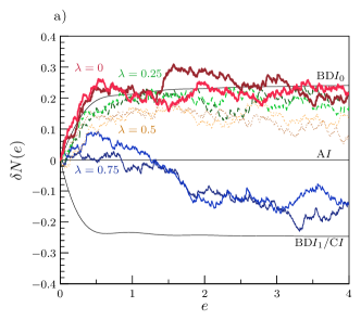
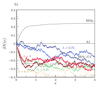
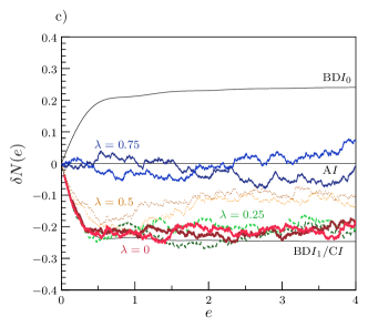
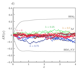
Figure 3: (Color online) Integrated deviation of the microscopic density of states for different values of the coupling parameter (fat red lines for $\lambda=0$, dashed green lines for $\lambda=0.25$, dotted yellow lines for $\lambda=0.5$ and thin blue lines for $\lambda=0.75$). Thin black lines correspond to random-matrix predictions for the indicated symmetry classes. Graph a) shows the spectra of the blocks $H_{++}$ and $H_{-+}$ that belong to symmetry class BD$I_{0}$, i.e. for integer $j$ and even dimensional invariant subspaces (each curve combines 280 spectra). Graph b) shows spectra of the same blocks $H_{++}$ and $H_{-+}$ that belong to symmetry class BD$I_{1}$, i.e. integer $j$ and odd dimensional subspaces (again 280 spectra per line). Graph c) shows the spectra of $H_{++}$ and $H_{-+}$ in symmetry class C$I$, i.e. half-integer $j$ (560 spectra per line). Graph d) shows the spectra for the blocks $H_{+-}$ and $H_{--}$ that belong to the standard Wigner-Dyson class A$I$ where integer and half-integer values of $j$ have been combined separately (560 spectra per line).

such that all nontrivial signatures are contained in $\delta d(e)$. In Figure 3 we plot the integrated version

$$\delta N(e)=\int_{0}^{e}\delta d(e^{\prime})\ de^{\prime}.$$ (32)

The graphs support the generalized BGS conjecture in that they follow the symmetry class specific signatures as predicted by the Gaussian random-matrix ensemble for the corresponding symmetry classes if the classical dynamics is chaotic at $\lambda=0$ and $\lambda=0.25$. The signatures become weaker if the classical dynamics is mixed $\lambda=0.5$ and disappear or change further in the near-integrable case $\lambda=0.75$. We do not show the fully integrable case $\lambda=1$ which is highly degenerate and ungeneric both classically and quantum mechanically. For the spectra in the standard symmetry classes no signatures are expected irrespective of the classical dynamics. This is confirmed in Figure 3 d).

Let us next turn to the distribution $P_{1}(e)$ of the first positive eigenvalue. Numerically we will consider the integrated distribution

$$I(e)=\int_{0}^{e}P_{1}(e^{\prime})de^{\prime}.$$ (33)

$E(e)=1-I(e)$ is also known as the gap probability. In the three Wigner-Dyson classes this can be calculated directly from the level spacing distribution $P(s)$

$$I(e)=\int_{0}^{e}sP(s)ds+e\int_{e}^{\infty}P(s)ds$$ (34)

For the GOE the level-spacing distribution is given by Wigner surmise (up to very small corrections that are beyond our numerical analysis)

$$P(s)=\frac{\pi}{2}\exp\left({-\frac{\pi}{4}s^{2}}\right)\ .$$ (35)

This leads to

$$I_{\mathrm{GOE}}(e)=\mathrm{erf}\left(\frac{\sqrt{\pi}}{2}e\right)$$ (36)

which is the prediction for quantum chaotic spectra in class A$I$ (modulo above mentioned tiny corrections). Integrable systems in any of the Wigner-Dyson classes have Poissonian spectra with $P(s)=e^{-s}$. The prediction for integrable systems in class A$I$ is then

$$I_{\mathrm{Poisson}}(e)=1-\exp(-e)\ .$$ (37)

For $e\to 0$ both, the GOE and the Poisson prediction behave like $I(e)\sim e$ which is consistent with a featureless density of states $d(e)=1$. The stronger spectral rigidity of quantum chaotic spectra versus integrable systems can be seen from the much quicker saturation $I_{\mathrm{GOE}}(e)\to 1$ compared to the Poissonian case. In the nonstandard symmetry classes predictions for quantum chaotic spectra are obtained from the well-known joint-probability distributions of eigenvalues of the corresponding Gaussian ensembles of random-matrix theory (a very useful overview of all relevant information can be found in the Appendix of kieburg ). In class BD$I_{0}$ one has

$$I_{\mathrm{BD}I_{0}}(e)=1-\exp\left(-\frac{\pi^{2}}{8}e^{2}-\frac{\pi}{2}e\right)\ .$$ (38)

The attraction of eigenvalues to $e=0$ shows in the steeper behavior $I_{\mathrm{BD}I_{0}}(e)\sim\frac{\pi}{2}e$. In the classes BD$I_{1}$ and C$I$ one has (again) the same prediction

$$I_{\mathrm{BD}I_{1}}(e)=I_{\mathrm{C}I}(e)=1-\exp\left(-\frac{\pi^{2}}{8}e^{2}\right)$$ (39)

which show level repulsion from $e=0$ as $I(e)\sim\frac{\pi^{2}}{8}e^{2}$ only grows quadratically.

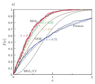
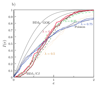
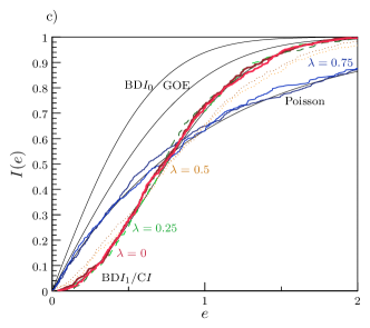
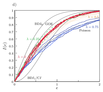
Figure 4: (Color online) Integrated distribution of the first positive eigenvalue. The description of individual curves and graphs of Fig. 3 applies here analogously.

In Figure 4 we compare the random-matrix predictions to the numerical data for the various symmetry classes realized in different subspaces. Again we find support of the generalized BGS conjecture. The spectra in quantum chaotic cases $\lambda=0$ and $\lambda=0.25$ follow the corresponding random-matrix prediction and we see a crossover to Poissonian statistics in the mixed dynamics case $\lambda=0.5$ and the near-integrable case $\lambda=0.75$. The distinct signatures of the nonstandard classes are very clear as the fluctuations are much smaller than the difference between the various predictions.

V Conclusions

We have shown that the Feingold-Peres model of two coupled tops belongs to nonstandard symmetry classes and we numerically analyzed their spectra in a crossover where the corresponding classical dynamics changes from chaotic to mixed and near-integrable. For chaotic classical dynamics the spectral fluctuation near the spectral symmetry point $E=0$ show the characteristic signatures of nonstandard symmetry classes as predicted by the corresponding Gaussian ensembles of random-matrix theory: levels are repelled or attracted to $E=0$ depending on the nonstandard symmetry class while the standard Wigner-Dyson classes do not have a spectral symmetry point and show no attraction or repulsion from $E=0$. The signatures can very clearly be seen by looking at the density of states (or its integral the spectral counting function) or the (integrated) distribution of the first positive eigenvalue. For nonchaotic classical dynamics these signatures either disappear or change drastically.
This gives numerical support for a generalized BGS conjecture, that chaos in the classical dynamics implies universal spectral statistics that only depends on the symmetry classification according to the Altland-Zirnbauer tenfold way. Our analysis is a further step in understanding the specific spectral signatures related to nonstandard symmetry classes. Two obvious directions for future work are

1. the extension to other symmetry classes that are not covered by the Feingold-Peres Hamiltonian (1),

2. the semiclassical analysis based on periodic-orbit theory in the Gutzwiller trace formula.

Let us mention a few words on both directions.
Currently there is only a restricted set of paradigm models for quantum chaos in nonstandard symmetry classes available in the literature. Magnetic Andreev billiards provide a model in class C and the present work adds models for classes BD$I$ and C$I$. It is in principle not difficult to construct Hamiltonians for two couples tops that generalize the Feingold-Peres model to other nonstandard symmetry classes. For such a constructions one may make a choice of the appropriate chirality, charge conjugation or time-reversal operators for a given symmetry class. Then one writes down all monomial combinations of the angular momentum components that are consistent with the symmetry and chooses a linear combination as a family of Hamiltonians. One may also generalize by allowing the total angular momentum quantum numbers of the two tops to be different $\mathbf{L}^{2}\equiv j_{1}(j_{1}+1)$ and $\mathbf{M}^{2}\equiv j_{2}(j_{2}+1)$. As an example let us chose the standard time reversal operator, i.e. the antiunitary operator $T$ that reverses each angular momentum $T\mathbf{L}T^{-1}=-\mathbf{L}$ and $T\mathbf{M}T^{-1}=-\mathbf{M}$. Then $T^{2}=(-1)^{2(j_{1}+j_{2})}=\pm 1$ depending on whether $j_{1}$ and $j_{2}$ are both integer ($T^{2}=1$) both half-integer (also $T^{2}=1$) or one is integer and the other half-integer ($T^{2}=-1$). Next let us choose the unitary chirality operator $C=e^{i\pi M_{x}}$ which satisfies $TCT^{-1}=C$ and obeys $C^{2}=(-1)^{2j_{2}}=\pm 1$ depending on whether $j_{2}$ is integer ($C^{2}=1$) or half-integer ($C^{2}=-1$). The set of Hamiltonians

$$H=\frac{M_{y}}{j_{2}+1/2}\frac{a_{x}L_{x}+a_{y}L_{y}+a_{z}L_{z}}{j_{1}+1/2}+\frac{M_{z}}{j_{2}+1/2}\frac{b_{x}L_{x}+b_{y}L_{y}+b_{z}L_{z}}{j_{1}+1/2}+\frac{M_{x}\left(c_{y}M_{y}+c_{z}M_{z}\right)}{(j_{2}+1/2)^{2}}$$ (40)

where $a_{x}$, …, $b_{x}$, …, $c_{y}$ and $c_{z}$ are real coupling constants then obeys $CHC^{-1}=-H$ and $THT^{-1}=H$. Any unitary symmetry may be broken by changing some of the coupling constants such that further reduction is generally not necessary. Four different nonsymmetry classes are realized generically depending on $j_{1}$ and $j_{2}$: if $j_{1}$ and $j_{2}$ are both integer the symmetry class is again BD$I$, if they are both half-integer then it is C$I$, if $j_{1}$ is integer but $j_{2}$ half-integer, then we have D$III$, and if $j_{1}$ is half-integer and $j_{2}$ integer, then one gets C$II$. It is not difficult to see that all ten symmetry classes can be realized by generalizing the Feingold-Peres model in this way. This leads to a large set of potential paradigm models. The corresponding classical limit is obtained by taking $j_{1}\to\infty$ and $j_{2}\to\infty$ in an appropriate way. However, any detailed future quantum chaos analysis of these models may have to start with scanning the parameter space for full classical chaos or mixed dynamics.
The second direction mentioned above is the semiclassical periodic orbit approach based on the Gutzwiller trace formula which expresses the microscopic density of states as a sum

$$d(e)=1+\left\langle\sum_{p}A_{p}e^{iS_{p}/\hbar}\right\rangle$$ (41)

of a Weyl part that reduces to the unit constant (energies are measured in units of the mean level spacing) and a sum over periodic orbits $p$ of the corresponding classical dynamics. Each periodic orbit contributes a complex amplitude $A_{p}e^{iS_{p}/\hbar}$ where $S_{p}$ is the classical action $S_{p}=\oint\mathbf{P}\cdot d\mathbf{Q}$ of the periodic orbit and $A_{p}$ may be expressed in terms of the classical stability of the orbit. The average $\langle\cdot\rangle$ is a running average over values of $\hbar$ while one consider the semiclassical limit $\hbar\to 0$. Only periodic orbits whose total action is very small can contribute. For standard symmetry classes there is no mechanism for getting arbitrarily small classical actions and the sum over periodic orbit does not survive the average. In the presence of a nonstandard symmetry there is however a classical transformation corresponding to the quantum chiral or charge conjugation symmetry. This maps the energy shell $e=0$ into itself such each periodic orbit $p$ in the shell $e=0$ is mapped into a partner orbit $p^{\prime}$. If $p=p^{\prime}$ the periodic orbit is called self-dual. For magnetic Andreev billiards MagneticAndreev it has been shown that the total action $S_{p}$ of a self-dual orbit vanishes and that semiclassical sum rules may be applied to sum over all amplitudes $A_{p}$ of self-dual orbits. The resulting self-dual approximation is analogous to Berry’s well-known diagonal approximation for the semiclassical two-point correlation function diagonal . The self-dual approximation can be performed in all nonstandard symmetry classes for quantum graphs stargraphII . In the present case of two coupled tops it is not immediately obvious that the self-dual approximation is consistent with the Gaussian random-matrix predictions. We hope that future work will clarify this in detail.

Appendix A Explicit derivation of the topological index

In this appendix we assume that $j$ is integer and show that the topological index of the reduced Hamiltonian $H_{++}$ is $\nu_{++}=0$ if $j$ is odd and $\nu_{++}=1$ if $j$ is even. The corresponding statement for $H_{-+}$ ($\nu_{-+}=0$ if $j$ is even and $\nu_{-+}=1$ if $j$ is odd) may be proven in analogously.
From $C|m_{1},m_{2}\rangle=(-1)^{j-m_{2}}|-m_{1},-m_{2}\rangle$ we can find the action of the reduced chirality operator $C_{++}$ as

$$C_{++}|m_{1},m_{2},++\rangle=(-1)^{j-m_{2}}|-m_{2},-m_{1},++\rangle$$ (42)

where we have used that $m_{1}+m_{2}$ is even in the subspace $V_{++}$. If $m_{1}\neq-m_{2}$, then we find the eigenstates

$$C_{++}\left(|m_{1},m_{2},++\rangle+|-m_{2},-m_{1},++\rangle\right)= =(-1)^{j-m_{2}}\left(|m_{1},m_{2},++\rangle+|-m_{2},-m_{1},++\rangle\right)$$ (43a)

$$C_{++}\left(|m_{1},m_{2},++\rangle-|-m_{2},-m_{1},++\rangle\right)= =(-1)^{j-m_{2}+1}\left(|m_{1},m_{2},++\rangle-|-m_{2},-m_{1},++\rangle\right)$$ (43b)

which have pairwise eigenvalues $\pm 1$ and so do not contribute to the topological index.
If $m_{1}=-m_{2}$ then (42) implies

$$C_{++}|m_{1},-m_{1},++\rangle=(-1)^{j+m_{1}}|m_{1},-m_{1},++\rangle$$ (44)

with eigenvalues $(-1)^{j+m_{1}}$. As $m_{2}\geq m_{1}$ and $m_{1}+m_{2}$ are even for $V_{++}$ where $m_{1}$ runs over the $j+1$ values $m_{1}=-j,-j+1,\dots,0$. The alternating signs of the eigenvalues then imply that the topological index is $\nu_{++}=1$ if $j$ is even, and $\nu_{++}=0$ if $j$ is even as claimed.

- (1) M. Feingold, A. Peres, Physica 9D, 433 (1983).
- (2) M. Feingold, N. Moiseyev, A. Peres, Phys. Rev. A 30, 509 (1984).
- (3) A. Altland, M.R. Zirnbauer, Phys. Rev. Lett. 76, 3420 (1996).
- (4) A. Altland, M.R. Zirnbauer, Phys. Rev. B 55, 1142 (1997).
- (5) M.R. Zirnbauer, J. Math. Phys. 37, 4986 (1996).
- (6) E.P. Wigner, Proc. Cambridge Philos. Soc. 47, 790 (1951)
- (7) E.P. Wigner, Ann. Math. 67, 325 (1958).
- (8) F.J. Dyson, J. Math. Phys. 3, 140 (1962).
- (9) F.J. Dyson, J. Math. Phys. 3, 1199 (1962).
- (10) J.J.M. Verbaarschot, I. Zahed, Phys. Rev. Lett. 70, 3852 (1993).
- (11) J.J.M. Verbaarschot, Phys. Rev. Lett. 72, 2531 (1994).
- (12) R. Gade, Nucl. Phys. B 398, 499 (1993).
- (13) K. Slevin, T. Nagao, Phys. Rev. Lett. 70, 635 (1993).
- (14) J. Wishart, Biometrika 20A, 32 (1928).
- (15) S. Gnutzmann, B. Seif, Phys. Rev. E 69, 056219 (2004).
- (16) O. Bohigas, M.J. Giannoni, C. Schmit, Phys. Rev. Lett. 52, 1 (1984).
- (17) M.V. Berry, Proc. R. Soc. Lond. A 400, 299 (1985).
- (18) N. Argaman, F.M. Dittes, E. Doron, J. Keating, A. Kitaev, M. Sieber, U. Smilansky, Phys. Rev. Lett. 71, 4326 (1993).
- (19) M. Sieber, K. Richter, Phys. Scr. T90, 128 (2001).
- (20) S. Gnutzmann, A. Altland, Phys. Rev. Lett. 93, 194101 (2004).
- (21) S. Gnutzmann, A. Altland, Phys. Rev. E 72, 056215 (2005).
- (22) S. Gnutzmann, U. Smilansky, Adv. Phys. 55, 527 (2006).
- (23) S. Müller, S. Heusler, A. Altland, P. Braun, F. Haake, New J. of Phys. 11, 103025 (2009).
- (24) A. Altland, S. Gnutzmann, F. Haake, T. Micklitz, Rep. Prog. Phys. 78, 086001 (2015).
- (25) J.P. Keating, Nonlinearity 4, 309 (1991).
- (26) E. B. Bogomolny, B. Georgeot, M. J. Giannoni, C. Schmit, Physics Reports 291, 219 (1997).
- (27) M.V. Berry, M. Robnik M, J. Phys. A 17, 2413 (1984).
- (28) S. Gnutzmann, B. Seif, Phys. Rev. E 69, 056220 (2004).
- (29) S. Gnutzmann, B. Seif, F. von Oppen, M.R. Zirnbauer, Phys. Rev. E67, 046225 (2003).
- (30) I. Kosztin, D.L. Maslov, P.M. Goldbart, Phys. Rev. Lett. 75, 1735 (1995).
- (31) C.W.J. Beenakker, Lecture Notes in Physics 667, 131-174 (2005).
- (32) J.J.M. Verbaarschot, Nucl.Phys. B426, 559 (1994).
- (33) D.A. Ivanov, J. Math. Phys. 43, 126 (2002).
- (34) A. Edelman, Lin. Alg. Appl. 159, 55 (1991).
- (35) M. Kieburg, T.R. Würfel, Phys. Rev. D 96, 034502 (2017).