Spectroscopic confirmation of very-wide stellar binaries and large-separation comoving pairs from Gaia DR1

Abstract

Members of widely-separated stellar binaries ($\gtrsim 0.1$ pc) or loosely bound stellar associations and clusters are born with small spreads in kinematics and chemistry, but disrupt and dissociate on timescales comparable to their orbital time within the Milky Way. The kinematic properties of comoving star pairs—bound wide binaries or unbound but coeval stars—are therefore sensitive to both the smooth tidal field and gravitational perturbation spectrum of the Milky Way. In previous work, we identified $>4,000$ candidate comoving pairs using only astrometric data from the Tycho-Gaia Astrometric Solution (TGAS) catalog and find a large number of pairs with separations $\gtrsim 1~{}\mathrm{pc}$. Without radial velocity measurements for the vast majority of these pairs, the false-positive rate at these separations is significant ($\sim 50\%$). Here we present results from our own low-resolution radial-velocity survey of a random sample of the candidate pairs to identify and validate true comoving star pairs. Of the 311 observed comoving pairs, we confirm 127 comoving pairs with separations as large as $\approx 10~{}\mathrm{pc}$, our original search limit. At separations of $10^{-3}~{}\mathrm{pc}$ to $\approx 0.5~{}\mathrm{pc}$, the number of confirmed pairs per separation decreases with increasing separation (number per log separation is uniform). From $\approx 0.5~{}\mathrm{pc}$ to $10~{}\mathrm{pc}$, the number per separation is approximately uniform (number per log separation increases). We confirm the discovery of a population of comoving star pairs at very large separations, suggesting that disrupted wide binaries and stellar associations remain approximately spatially coherent.

Section 1 Introduction

Widely-separated, coeval star pairs or multiples — i.e. wide binaries, multiplets, or former binaries or multiplets — are important tracers of many processes that formed and continue to shape the Milky Way. They have been used to place limits on the mass distribution and population of massive perturbers in the Galaxy (e.g., Yoo et al. 2004; Monroy-Rodríguez & Allen 2014), to study the physics of star formation (e.g., Parker et al. 2009; Reipurth & Mikkola 2012), and to calibrate stellar models and inferences across the main sequence (e.g., Brewer et al. 2016). These examples represent a small subset of a much broader range of applications (see, e.g., Chanamé 2007).

At smaller separations ($\lesssim 0.1~{}\mathrm{pc}$), comoving pairs of stars are likely bound wide binaries. It has long been recognized that the observed period or separation distribution of these low-binding-energy binaries encapsulates information about the Galactic mass distribution (Öpik 1924; Oort 1950; Bahcall et al. 1985). In particular, early simulations of populations of wide binaries showed that the expected separation distribution, $p(s)$, for $0.01<s<1~{}\mathrm{pc}$ tends to follow a power law, $p(s)\propto s^{-\alpha}$ for $\alpha\approx 1$–$2$, with a possible steep break that depends on the details of the population of massive perturbers in the Galaxy, i.e. giant molecular clouds (GMCs), black holes, etc. (Weinberg et al. 1987).

At larger separations ($\gtrsim 0.1~{}\mathrm{pc}$), comoving pairs are likely a mix of tenuously bound stars such as recently disrupted binaries, moving groups or resonant features, and the final products of dissolving stellar associations or clusters. However, even at separations of $\sim 0.1~{}\mathrm{pc}$, we typically lack the velocity or distance precision to determine the binding energy of a system and therefore can’t determine its true dynamical state; because of this ambiguity, we refer to both bound and unbound widely-separated ($\gtrsim 10^{-3}~{}\mathrm{pc}$) systems collectively as “comoving” systems.

Primarily thanks to large astrometric surveys and catalogs (ESA 1997; Lépine & Shara 2005; Gaia Collaboration et al. 2016b) and radial-velocity surveys (Steinmetz et al. 2006), several hundred confirmed comoving star pairs (Shaya & Olling 2011) and over 4,000 candidate systems (Gould & Chanamé 2004; Lépine & Bongiorno 2007; Tokovinin & Lépine 2012; Allen & Monroy-Rodríguez 2014; Oh et al. 2017; Oelkers et al. 2017; Andrews et al. 2017) have been discovered over the last several decades (see also Chanamé 2007 and references therein). These pairs are identified by searching for approximately cospatial stars that appear to be comoving either in sky-projected velocities — we refer to these as “comoving pair candidates” — or using full-space velocity information — we refer to these as “confirmed comoving pairs.” Radial velocity follow-up is still needed to confirm the majority of the known candidates, though Gaia DR2 will provide radial velocities for the brightest stars ($G<12$; Gaia Collaboration et al. 2016b).

With large samples of candidate pairs, several groups have measured the separation distribution of wide binaries at angular separations $\Delta\theta\lesssim 1^{\circ}$ where the false-positive rate is expected to be lower and the samples are likely predominantly wide binaries (Chanamé & Gould 2004; Lépine & Bongiorno 2007; Sesar et al. 2008). In most cases, the angular or projected separation distribution is fit using a decreasing power-law, and the power-law index, $\alpha$, is found to be $\alpha\approx 1.5$–$2$ out to angular separations of $\approx 0.25^{\circ}$ ($\approx 0.65~{}\mathrm{pc}$ at a distance of $150~{}\mathrm{pc}$), apparently consistent with simulations (e.g., Weinberg et al. 1987). Tentative reports of a steepening or cutoff of the separation distribution at larger separations have been claimed (e.g., Yoo et al. 2004; Quinn et al. 2009), but these claims are limited by small numbers of confirmed pairs at large separations.

Most measurements of the separation distribution have neglected the possible existence of larger separation ($\gtrsim 1~{}\mathrm{pc}$) unbound or ionized pairs. Early theoretical work either explicitly ignored these stars (e.g., Weinberg et al. 1987), or suggested that unbound stars would drift and no longer remain spatially coherent within one Galactic orbit (e.g., see Appendix in Yoo et al. 2004). More recent simulations of the disruption and evolution of wide binary populations include an approximation of the Galactic tidal field and instead predict that ionized binaries could appear as a second peak or component in the separation distribution of comoving stars at much larger separations (10–$1000~{}\mathrm{pc}$; Jiang & Tremaine 2010). Though these simulations don’t include perturbers like GMCs or black holes, they at least indicate that disrupted wide binaries may remain coherent for a longer period of time than previously thought. Thus, a monotonically decreasing separation distribution may be too simple of a model for the separation distribution of comoving stars in our Galaxy. In addition, the distribution of unbound but comoving stars should be very sensitive to diffusive processes that determine the rate at which the pairs separate.

Indeed, observational work that followed appears to find tentative evidence for the existence of a second peak in the separation distribution of radial-velocity-confirmed comoving stars (Shaya & Olling 2011; hereafter SO11). A key aspect of this work was to move from searching for common proper motion pairs to performing a statistical inference of the difference in full-space velocity vector for pairs of stars. At separations of $1$–$10~{}\mathrm{pc}$, star pairs in the local solar neighborhood subtend large angles on the sky: even if the two component stars were moving with the same 3D velocity, their proper motions and radial velocities can be different. By compiling radial velocities from the literature for Hipparcos stars, SO11 applied this method to search for all comoving star pairs with separations larger than $0.01~{}\mathrm{pc}$ within $100~{}\mathrm{pc}$ of the sun. They find $\sim 200$ high probability comoving pairs with a separation distribution that falls of until $\sim 1~{}\mathrm{pc}$, where the number of pairs then begins rising in bins of log-separation.

To verify the existence of a population of very wide-separation comoving pairs, we first need to identify a large sample of confirmed comoving stars. This will already be possible for the brightest stars with Gaia DR2, but obtaining even larger samples will require significant efforts to obtain radial velocities for candidate comoving pairs. In this work, we present a catalog of confirmed comoving star pairs discovered through low-resolution spectroscopic follow-up of candidate comoving stars selected from inferences using astrometric measurements from the TGAS catalog alone (Oh et al. 2017).

We describe the data and observations in Section 2. Details of the spectroscopic reduction and velocity measurements are described in the Appendix. We present our main results in Section 3 and Section 4.

Section 2 Data

Figure 1: Color-magnitude diagram for all TGAS sources within $200~{}\mathrm{pc}$ (background blue histogram) and all comoving star pair members observed in this follow-up effort (black points); colored lines connect candidate comoving star pairs. 2MASS (Skrutskie et al. 2006) $J$-band magnitudes are obtained from the Gaia science archive. Apparent $G$-band magnitudes (Carrasco et al. 2016) are converted to absolute magnitude, $M_{G}$, using a Lutz-Kelker-corrected (Lutz & Kelker 1973) distance estimate (see also Equation 1 in Oh et al. 2017).

2.1 Sample selection

In previous work, we have identified a sample of high-confidence, candidate comoving star pairs (Oh et al. 2017) using only astrometric information from the TGAS catalog (Michalik et al. 2015; Gaia Collaboration et al. 2016a). These comoving pairs were selected using a cut on a marginalized likelihood ratio computed for all nearly co-spatial pairs of stars. We performed a model selection between two hypotheses: that the velocities of the two stars in a pair are identical (case 1) or that they are indepndent (case 2). We marginalized over the (unknown) true velocity and distance of each star to obtain the ratio of fully marginalized likelihoods, $\mathcal{L}_{1}/\mathcal{L}_{2}$. The likelihoods appropriately take into account the reported uncertainties and covariances of the astrometric measurements in the TGAS catalog as well as projection effect in comparing spherical velocities for star pairs separated by large angles on the sky.

After a parallax signal-to-noise ratio (SNR) cut, $\varpi/\sigma_{\varpi}>8$, we compute the marginalized likelihood ratio for all stars within $10~{}\mathrm{pc}$ and with a difference in tangential velocity $\Delta v_{\perp}<10~{}\mathrm{km}~{}\mathrm{s}^{-1}$ for each star in the TGAS catalog. After applying a conservative cut on the likelihood ratio motivated by computing the same likelihood ratio for random pairings of stars, $\ln\mathcal{L}_{1}/\mathcal{L}_{2}>6$, we found 13,058 comoving star pairs with physical separations between $10^{3}~{}\mathrm{au}$ and $10~{}\mathrm{pc}$. Of these pairs, there are 10,606 unique sources, implying that a significant fraction of the identified pairs are members of larger groups. However, we have also found a large number ($\approx$4,000) of mutually-exclusive linked pairs that increase in number with increasing log-separation from $\sim 1$ $\mathrm{pc}$. For a full description of the selection method, see Oh et al. 2017.

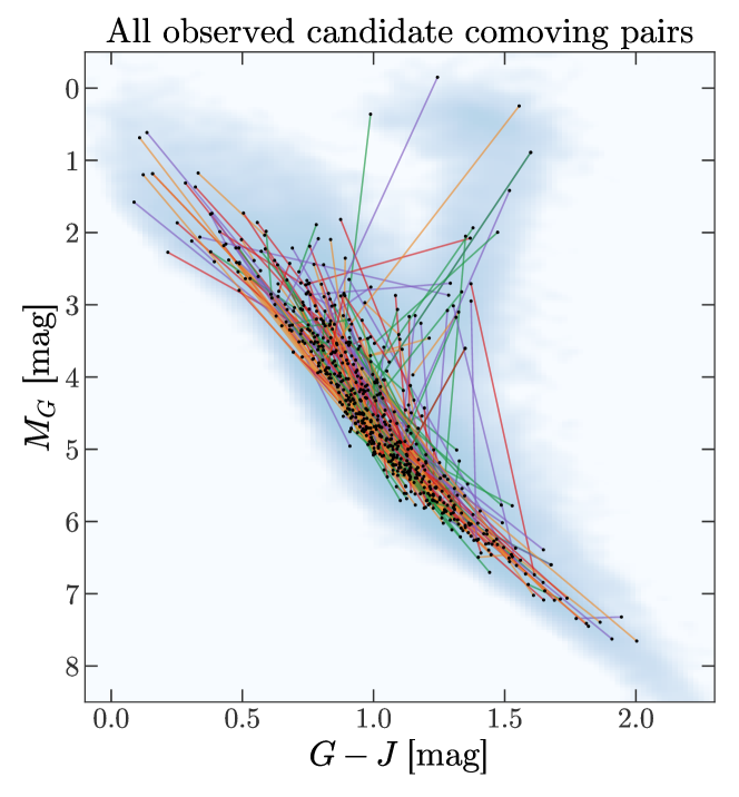
To select candidate pairs for follow-up spectroscopic observations, we only consider mutually exclusive star pairs within $200~{}\mathrm{pc}$ in Heliocentric distance. With the SNR cut used above and given the limitations of the TGAS catalog itself, TGAS is $\approx$90% complete to $200~{}\mathrm{pc}$ (Bovy 2017). From this source target list, we randomly observed targets with airmass $\sec z<1.5$ during our observing run. Figure 1 shows a color-magnitude diagram of all targets observed in this observing run (markers) plotted over the density of all TGAS stars within $200~{}\mathrm{pc}$. Candidate comoving pairs are connected by (colored) lines.

2.2 Observations and data reduction

Spectra were obtained using the Modspec spectrograph mounted on the $2.4~{}{\rm m}$ Hiltner telescope at MDM observatory on Kitt Peak (Arizona). Modspec was set up in long-slit mode with a 1″ slit, a $600~{}{\rm line}~{}{\rm mm}^{-1}$ grating, and a $2048\times 2048~{}{\rm pixel}$ SITe CCD detector (“Echelle”). Only the central 300 pixel columns were read out from the CCD, and pixel rows $>1600$ (at the blue end) were later trimmed because of the poor quantum efficiency of the CCD at wavelengths $\lesssim 3600~{}{\rm\AA}$. The resolution and wavelength range were $\approx 2~{}{\rm\AA}~{}{\rm pixel}^{-1}$ from $\approx 3600$–$7200~{}{\rm\AA}$. At this resolution, to obtain high signal-to-noise ($>100$ per pixel) spectra, most exposures were between $30$–$120~{}{\rm s}$. To maximize the number of observed pairs, we chose not to take comparison lamp spectra at each pointing as it adds an overhead of $\approx 90~{}{\rm s}$ per observation. We are primarily interested in relative velocities between pair members and therefore don’t need precise absolute calibrations of their radial velocities. To determine rough nightly wavelength solutions, calibration spectra were obtained using Hg-Ne and Ne comparison lamps at the beginning and end of each night. Additionally, atmospheric emission lines were used to correct the wavelength solution on a per-object basis.

We observed a total of 765 unique sources over 5 nights from (UT) 2017-03-11 to 2017-03-15, corresponding to 323 unique pairs and $\approx 120$ calibration targets. All calibration targets have previously measured radial velocities from high-resolution spectroscopic surveys (Bensby et al. 2014; Pinsonneault et al. 2014) in order to validate our radial velocity measurements. These stars also have measured chemical abundances, and will be used in future work as a training set for The Cannon (Ness et al. 2015) to infer metallicities and stellar parameters for our observed sources. The spectra were reduced and calibrated using a custom, publicly-available pipeline written in Python; see Appendices A–C for a full description of the data reduction procedure.

2.3 Validation of absolute radial velocities

Several of our targets and all of our calibration targets have previously measured radial velocities (RVs). We can therefore estimate the absolute velocity uncertainties by comparing our derived radial velocities with high-quality prior measurements. For calibration sources, we use radial velocity values reported in the source catalogs (Bensby et al. 2014; Pinsonneault et al. 2014). For all other sources, following previous work (Shaya & Olling 2011), we search for previous RV measurements (in decreasing order of priority) with:

1. The Geneva-Copenhagen Survey of the Solar Neighborhood (Nordström et al. 2004).

2. The Catalogue of Radial Velocities of Galactic Stars with Astrometric Data, the Second Version (Kharchenko et al. 2007).

3. The General Catalogue of Mean Radial Velocities (Barbier-Brossat & Figon 2000).

4. The SIMBAD database (Wenger et al. 2000). We use astroquery (Ginsburg et al. 2016) to retrieve records from the database, which do not contain uncertainties but do contain a quality flag. We only retain RVs that have a quality flag set to ‘A’ and adopt a $5~{}\mathrm{km}~{}\mathrm{s}^{-1}$ uncertainty for all such values.

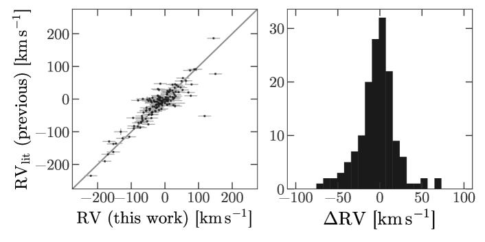
We find that 155 of the observed stars (mainly calibration targets) have reliable prior measurements from the literature search described above. Figure 2 shows the distribution of velocity differences between our measurements and literature values. From this distribution (right panel), we compute the median absolute deviation (MAD) and estimate the standard deviation to be $\approx 20~{}\mathrm{km}~{}\mathrm{s}^{-1}$, which we adopt as our global systematic error for all absolute radial velocities. We note, however, that for computing relative velocities for pairs of nearby stars, it is the RV precision (typically $\approx 5$–$10~{}\mathrm{km}~{}\mathrm{s}^{-1}$) that matters.

Figure 2: Comparison of radial velocities measured from our observations with radial velocities obtained from the literature search described in Section 2.3. Left panel shows our values on the $x$-axis, ${\rm RV}$, against the previous literature values on the $y$-axis, ${\rm RV}_{\rm lit}$, for 155 observed stars (mainly calibration targets) with previously measured radial velocities. Right panel shows a histogram of the differences, $\Delta{\rm RV}={\rm RV}-{\rm RV}_{\rm lit}$. The estimated standard-deviation of the difference distribution implies a global systematic uncertainty of $\approx 20~{}\mathrm{km}~{}\mathrm{s}^{-1}$.

Section 3 Results

3.1 Comoving pair catalog

Of the 323 observed star pairs, 12 have at least one member with an unreliable (flagged) radial velocity measurement from the spectroscopic reduction pipeline. For the remaining 311 pairs, we use the measured radial velocities to re-compute the marginal likelihood ratio for the two hypotheses considered in previous work (see Appendix B, Oh et al. 2017). We compute two fully marginalized likelihoods (FMLs) for the data: (1) assuming that the two stars are comoving with identical 3D velocity vectors (within some allowed small dispersion), and (2) assuming that the two stars have independent 3D velocity vectors drawn from a prior velocity distribution. We set the small allowed dispersion ($s$, in previous work) to $1~{}\mathrm{km}~{}\mathrm{s}^{-1}$, and use a mixture of three Gaussian velocity components for the prior, meant to represent the thin disk, thick disk, and halo velocity distributions relative to the sun (see Oh et al. 2017).

To compute the new likelihood ratio, we modify the expressions from Oh et al. (2017) to include the radial velocity measurements. In the same notation, this requires the following changes:

• The projection matrix, $\mathbf{M}$, now has to include the radial unit vector

  $$\mathbf{M}=\left(\begin{array}[]{c c c}-\sin\alpha&\cos\alpha&0\\ -\sin\delta\,\cos\alpha&-\sin\delta\,\sin\alpha&\cos\delta\\ \cos\delta\,\cos\alpha&\cos\delta\,\sin\alpha&\sin\delta\end{array}\right)$$ (1)

  where $(\alpha,\delta)$ are the ICRS coordinates (right ascension and declination) of a given star.

• The data-space velocity vector, $\boldsymbol{y}$, for one star now becomes

  $$\boldsymbol{y}={\left(\begin{array}[]{c c c}r_{i}\,\mu_{\alpha}^{*}&r_{i}\,\mu_{\delta}&v_{r}\end{array}\right)}^{\!\mathsf{T}}$$ (2)

  where $\mu_{\alpha}^{*}$ is the proper motion in right ascension (including the $\cos{\delta}$ term), $\mu_{\delta}$ is the proper motion in declination, and $v_{r}$ is the radial velocity.

• The covariance matrix becomes the block-diagonal matrix

  $$\mathbf{\Sigma}=\left(\begin{array}[]{c c}r^{2}\,\mathbf{C}&0\\ 0&\sigma_{v_{r}}^{2}\end{array}\right)$$ (3)

  where $r$ is the distance, $\mathbf{C}$ is the proper motion covariance matrix (from the TGAS catalog), and $\sigma_{v_{r}}$ is the radial velocity uncertainty.

To compute the FML for hypothesis 1 for a pair of stars $(i,j)$, the data-space vector must become the 6-vector

$$\boldsymbol{y}={\left(\begin{array}[]{c c}\boldsymbol{y}_{i}&\boldsymbol{y}_{j}\end{array}\right)}^{\!\mathsf{T}}$$ (4)

and the covariance matrix becomes the block-diagonal matrix

$$\mathbf{\Sigma}=\left(\begin{array}[]{c c}\mathbf{\Sigma}_{i}&0\\ 0&\mathbf{\Sigma}_{j}\end{array}\right)\quad.$$ (5)

Figure 3: Point estimate of the 3D velocity difference between two stars in a comoving pair, $|\boldsymbol{v}_{1}-\boldsymbol{v}_{2}|$, plotted against the change in log-likelihood-ratio computed when including radial velocity data. Error bars are shown for a few randomly-chosen, representative pairs and represent the 15th and 85th percentiles of velocity differences computed from samples from the error distributions of parallax, proper motion components, and radial velocity. The likelihood ratio increases (i.e. the belief that the stars are comoving becomes stronger) when the 3D velocity difference is small.

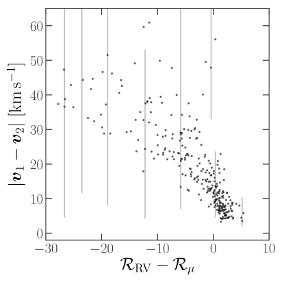
If the new likelihood ratio is larger than that computed from astrometry alone, the added radial velocity information supports the belief that the two stars are truly comoving in 3-space. Conversely, if the new likelihood ratio is smaller, the radial velocity data indicate that the pair is likely a false-positive and are not truly comoving. In practice, we compute the logarithm of the likelihood ratios, $\mathcal{R}=\ln\mathcal{L}_{1}/\mathcal{L}_{2}$; we refer to the proper-motion-only log-FML-ratio for a given pair of stars as $\mathcal{R}_{\mu}$ (as computed in Oh et al. 2017) and the log-FML-ratio including the radial velocity data as $\mathcal{R}_{\rm RV}$. We consider a pair as being genuinely comoving if $\mathcal{R}_{\rm RV}>\mathcal{R}_{\mu}$: 127 of the 311 comoving pairs satisfy this constraint. Figure 3 shows the magnitude of the 3D velocity difference plotted against the change in log-likelihood-ratio, $\mathcal{R}_{\rm RV}-\mathcal{R}_{\mu}$, for all observed pairs. In detail, for visualization, we sample from the error distributions over proper motion, parallax, and radial velocity for each star individually and compute the magnitude of the 3D velocity differences, $|\boldsymbol{v}_{1}-\boldsymbol{v}_{2}|$, for $2^{16}$ samples. We plot the median of the resulting distribution of velocity-differences as dark markers (circles). The error bars show the 15th and 85th percentiles of the distributions for a few randomly chosen pairs. Note that pairs with large 3D velocity differences have large (negative) changes to their log-likelihood-ratio values. Some pairs with large velocity differences also have small (near zero) changes to the log-likelihood ratio: these are pairs where each member has a velocity that is an outlier with respect to the prior velocity distribution.

The inferred 3D velocity differences and values for $\mathcal{R}_{\rm RV}$ and $\mathcal{R}_{\mu}$ for all observed candidate comoving pairs are provided with the associated table (Table 4; see Appendix D).

Figure 4: Point estimate of the 3D velocity difference between two stars in a comoving pair, $|\boldsymbol{v}_{1}-\boldsymbol{v}_{2}|$, plotted against a point estimate of the 3D spatial separation of the two stars, $|\boldsymbol{x}_{1}-\boldsymbol{x}_{2}|$. The distances used in the point estimates are computed using a Lutz-Kelker-corrected parallax value (Lutz & Kelker 1973).

3.2 Confirmed comoving pairs

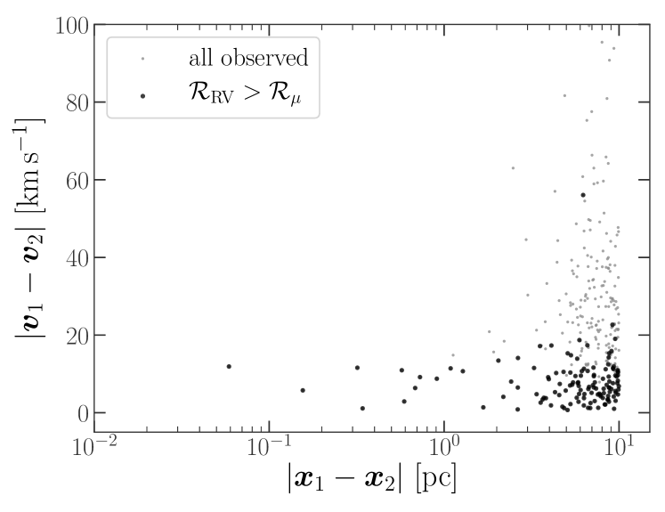
Figure 4 shows the magnitude of the 3D velocity difference plotted against the 3D positional separation of the two stars in all observed pairs from this work. We again plot the median of the velocity difference distribution, and here use the Lutz-Kelker-corrected distance estimate (Lutz & Kelker 1973) computed from the stars’ TGAS parallax measurements to compute the 3D positions of the two stars. Small, gray markers are pairs for which $\mathcal{R}_{\rm RV}<\mathcal{R}_{\mu}$, i.e. where the radial velocity measurements weaken or change our belief that a given pair is comoving. Larger, black markers are confirmed comoving pairs ($\mathcal{R}_{\rm RV}>\mathcal{R}_{\mu}$); note that many large-separation pairs have been ruled-out as comoving, but most small-separation pairs maintain their status as comoving.

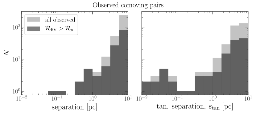
Figure 5 shows histograms of the spatial separation and sky separation for all pairs; background, gray histogram shows all observed pairs, and foreground, black histogram shows all pairs for which $\mathcal{R}_{\rm RV}>\mathcal{R}_{\mu}$. In this and subsequent figures, we use the phrase “tangential separation” (and symbol $s_{\rm tan}$) to refer to the chord length separation between the two pairs assuming the two stars are at the same distance (the smaller distance of the two, $d_{\rm min}$):

$$s_{\rm sky}=2\,d_{\rm min}\,\sin{\left(\frac{1}{2}\theta\right)}$$ (6)

where $\theta$ is the angular extent of the pair.

At sky separations $\gtrsim 1~{}\mathrm{pc}$, $\approx 40\%$ of the comoving pairs are confirmed to be comoving; interestingly, the separation distribution of the genuine pairs appears to be uniform or possibly growing in number with increasing separation. This strongly suggests the existence of a population of unbound wide binaries or dissolved open clusters, which maintain approximate spatial coherence for long times because of the small relative velocities at the time of disruption of the constituent stars (e.g., Jiang & Tremaine 2010). The kinematic properties of these unbound binaries and associations contain information about the tidal field and fluctuations in the mass distribution of the Milky Way. With Gaia DR2, we will be able to study the statistical properties of these widely-separated but comoving stars at even larger separations ($>10~{}\mathrm{pc}$).

Figure 5: Left: Distribution of point estimates of the 3D spatial separation of the stars in all observed comoving star pairs (gray), and only those confirmed as comoving (black). Note that the false-positive rate is $\approx 60\%$ at large separations ($>1~{}\mathrm{pc}$), but there are still a significant number of comoving pairs at these very wide separations. Right: Distribution of tangential separations for all comoving star pairs (gray) and only those identified as comoving with 3D velocity information (black). Noise in the parallax measurements makes the 3D separation distribution appear roughly uniform. Even the distribution in tangential separation appears to be approximately linear for large separations ($\gtrsim 0.1~{}\mathrm{pc}$).

Figure 6: Top: Distribution of tangential separation for all confirmed comoving star pairs, either from the radial velocity follow-up presented in this work or from RAVE DR5 radial velocities. At separations $\lesssim 10^{-1}~{}\mathrm{pc}$, the distribution (in log-log) appears uniform, consistent with past measurements of the wide binary separation distribution. At separations between $\approx 10^{-1}$–$10^{0}~{}\mathrm{pc}$, there appears to be an underabundance of comoving pairs, but the number of comoving pairs then begins to increase again out to our sample separation limit of $10~{}\mathrm{pc}$. Middle: Tangential separation plotted against mean distance for each comoving pair identified from this work (circles, blue) or from RAVE overlap (squares, orange). Right: Distance distribution for all confirmed comoving pairs. Note that at distances $\gtrsim 150~{}\mathrm{pc}$, our detection efficiency appears to decline.

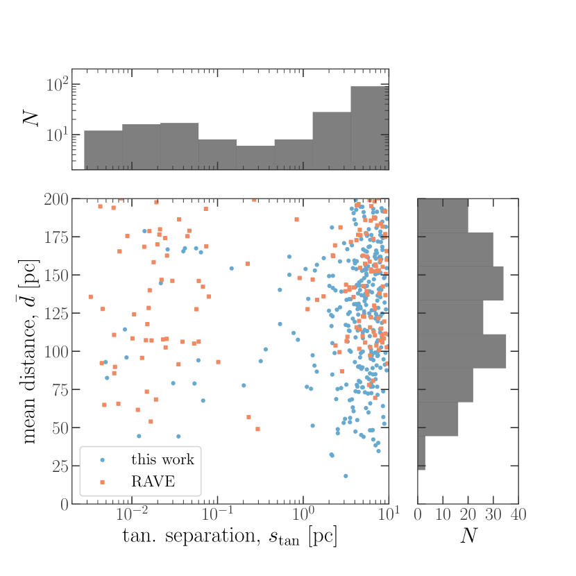
An additional 202 candidate comoving pairs (Oh et al. 2017) have previously-measured radial velocities (for each star) reported in DR5 of the Radial Velocity Experiment (RAVE; Kunder et al. 2017). Using the same procedure described in Section 3.1, we identify confirmed comoving pairs using the RAVE velocities for all pairs within $200~{}\mathrm{pc}$ and find a similar false-positive rate at large separations ($\approx 38\%$ are confirmed). Of the 154 RAVE-overlap candidate comoving pairs (within $200~{}\mathrm{pc}$) that meet the above criteria, we find 59 confirmed comoving pairs. We plot the confirmed comoving pairs identified through radial velocity follow-up in this work along with the RAVE-confirmed pairs in Figure 6. Top histogram shows the tangential separation distribution for the joint sample, scatter plot shows log-separation and the pair distances, and right histogram shows the distance distribution of the confirmed pairs. At larger distances ($\gtrsim 150~{}\mathrm{pc}$) it appears that the detection efficiency of our method drops, as expected given the hard cut in log-FML-ratio applied to define the candidate sample. Reassuringly, there do not appear to be any trends of the separation distribution with distance.

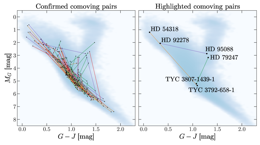
Figure 7 (left) shows the color-magnitude diagram for all confirmed comoving pairs. As would be expected if all of the pairs are coeval, the majority of pairs lie along isochrones in color-magnitude space, with the exception of a few visible outliers. For example, there appear to be at least a few main-sequence–giant-branch pairs, and a few pairs that appear to cross the main-sequence. We highlight a few of these pairs in the next section (Section 3.3).

Figure 7: Left: Color-magnitude diagram of confirmed comoving star pairs plotted over the density of all TGAS sources within 200 pc; similar to Figure 1, but for only the confirmed comoving pairs. Several interesting pairs that include main-sequence and giant component stars are highlighted in the text (Section 3.3) and in the right panel. Right: Same as left panel, but only three highlighted comoving star pairs are shown.

3.3 A few highlighted comoving pairs

Figure 7 (right) shows a few highlighted pairs selected from the color-magnitude diagram of confirmed comoving stars. We compile Tycho-2 ($B$, $V$; Høg et al. 2000), 2MASS ($J$, $H$, $K_{\rm s}$; Skrutskie et al. 2006), and WISE ($W_{1}$, $W_{2}$, $W_{3}$; Wright et al. 2010) photometry for each star in the pairs below and fit isochrones to the stars individually to measure their stellar parameters. We use the isochrones Python package (Morton 2015) to fit the photometric and parallax information (and uncertainties) for each star to infer the $\log g$, $T_{\rm eff}$, and stellar mass; these values are reported in Table 1. In brief, we use the model grids from the Dartmouth Stellar Evolution Database (Dotter et al. 2008) and the built-in interpolation in isochrones to compute the posterior probability of a given set of stellar parameters given the data (photometry and parallax). We generate samples (in stellar parameters) from this posterior pdf using the ensemble MCMC sampler implemented in emcee (Foreman-Mackey et al. 2013a) using 128 walkers. We run the sampler for 256 initial steps from random initial positions, compute the median position of the walkers in parameter-space and re-initialize the walkers in a small Gaussian ball around this median position to run for another 1024 burn-in steps. We then discard all but the last position and re-run for a final 8192 steps, saving only every 128th step. The stellar parameter values listed below are computed by taking the median posterior sample, and the uncertainties are estimated by computing the median absolute deviation, ${\rm MAD}$, and converting to a standard deviation under the assumption of Gaussianity ($\sigma\approx 1.5\times{\rm MAD}$).

Star name	$\log g$	$T_{\rm eff}$ [K]	mass [$M_{\odot}$]	tangential separation [pc]
HD 95088	$3.7\pm 0.02$	$5303\pm 74$	$1.490\pm 0.002$	$8.6\pm 0.8$
HD 92278	$4.2\pm 0.05$	$8519\pm 300$	$1.8\pm 0.1$
HD 79247	$3.61\pm 0.02$	$5075\pm 60$	$1.150\pm 0.004$	$6.8\pm 0.3$
TYC 3807-1439-1	$4.50\pm 0.04$	$5409\pm 80$	$0.88\pm 0.05$
HD 54318	$4.15\pm 0.04$	$10030\pm 345$	$2.4\pm 0.1$	$8.4\pm 1.1$
TYC 3792-658-1	$4.54\pm 0.03$	$5462\pm 139$	$0.89\pm 0.06$

Table 1: Stellar parameters inferred using isochrone-fitting for the three pairs highlighted in Section 3.3.

3.3.1 HD 95088 – HD 92278

From their surface gravities and temperatures, the component stars of this pair appear to be an A-type dwarf (HD 92278) and a slightly less massive G-type subgiant (HD 95088). This pair is separated by $4.5^{\circ}$ on the sky (corresponding to $\approx 8.6~{}\mathrm{pc}$ in tangential separation, see Table 1) and have consistent distances within their uncertainties of $\approx 110\pm 5~{}\mathrm{pc}$. At first glance, it seems unlikely that the two stars could be coeval, as the more massive A star has not begun its post-main-sequence evolution. One possible explanation is that this pair is a false-positive in three dimensions, in which case they are unassociated but just appear to be comoving with small relative velocity at present day.

Other speculative explanations for this pair stem from the possibility that it is the outcome of an interaction between even more stars. For example, an interaction between two wide binaries could result in an exchange of members, a hardening of one resulting binary, and a widening of the other binary (see, e.g., Leigh et al. 2016). Or, the initial system could have been an unstable three-body system that resulted in a tight inner binary and a wide outer binary; if the inner binary were close enough, it could have merged and formed a blue straggler star (e.g., Naoz & Fabrycky 2014), leaving the wide binary untouched.

High-resolution spectroscopy of these stars — and precise measurements of the stellar parameters and chemical abundances — may help to distinguish these scenarios.

3.3.2 HD 79247 – TYC 3807-1439-1

The components of this pair appear to be a K-type subgiant (HD 79247) and a G-type dwarf (TYC 3807-1439-1). This pair is separated by $4^{\circ}$ on the sky or $6.8~{}\mathrm{pc}$ in tangential separation and have an apparent radial separation of $\approx 3~{}\mathrm{pc}$, corresponding to a 3D separation of $\approx 9.8~{}\mathrm{pc}$ at a distance of $\approx 100~{}\mathrm{pc}$. Coeval stars at different phases of stellar evolution are extremely valuable for calibrating and testing stellar evolution models (e.g., Torres 2013). With a larger sample of confirmed comoving pairs, identified pairs that contain both an evolved star and a main sequence star — such as this pair — will be of great interest.

3.3.3 HD 54318 – TYC 3792-658-1

The components of this pair appear to be an A- or B-type dwarf (HD 54318) and a G-type dwarf (TYC 3792-658-1), the largest magnitude difference between all of the confirmed comoving pairs. This pair is separated by $2.5^{\circ}$ on the sky or $8.5~{}\mathrm{pc}$ in tangential separation and have a consistent distance of $\approx 190~{}\mathrm{pc}$ within their uncertainties. The mass ratio distribution of comoving star pairs will help constrain star formation models (e.g., Raghavan et al. 2010).

Section 4 Discussion

The results presented in this work demonstrate that even at separations larger than a parsec, a substantial fraction of comoving pair candidates selected from astrometry alone are confirmed with three-dimensional velocity information. This is exciting because it confirms the existence of what is likely a population of nearly-coherent but unbound coeval stars. It is also encouraging for the prospect of selecting large samples of comoving pairs purely with astrometric data from future data releases of the Gaia mission (radial velocity measurements will only be released for bright stars, $G<12$). However, in this work, we do not claim to report the true number or density of large-separation comoving pairs. To model the abundance and formation of comoving pairs, it will be crucial to select larger samples of pairs without hard cuts on separation, tangential velocity, signal-to-noise, or likelihood ratio, as were done with the input sample used in this work. It will also be important to quantify the contamination rate of (3D) comoving pair lookalikes, especially at large separations.

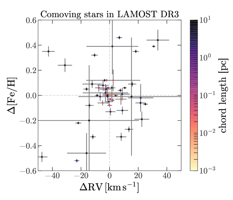
We do not try to estimate a contamination rate in this work, but instead use metallicities and radial velocities from 61 candidate comoving pairs that are in DR3 of the LAMOST survey (Deng et al. 2012) as an additional validation test. Figure 8 shows these pairs plotted as the difference in radial velocity and difference in iron abundance with points colored by the tangential separation of each pair. There is a clear over-density of pairs with abundance and radial-velocity differences close to zero. From this figure it is also clear that the false positives are predominantly the largest separation pairs (i.e. are the darkest markers), but a number of $>1~{}\mathrm{pc}$ pairs appear to have small radial-velocity differences and small differences in iron abundances, making them even more likely to be genuine pairs.

Figure 8: Differences in metallicity and radial velocity for candidate comoving pair member stars from the LAMOST survey. Points represent each pair, colored by the tangential separation, and error bars represent the uncertainties taken from the LAMOST DR3 catalog. There is a clear over-density of pairs with near-zero differences in metallicity and radial velocity even at large ($>1~{}\mathrm{pc}$) separations, adding even more confidence to the existence of comoving star pairs with these extreme separations.

Going forward, definitive confirmation of comoving star pairs may require precise measurements of chemical abundances combined with precise radial velocities, as demonstrated with the LAMOST data. However, we would also like to test assumptions about chemical homogeneity, rather than simply assuming that all true comoving pairs must have identical abundances. For example, the outcomes of planet formation may lead to large or appreciable abundance differences between coeval stars (e.g., Pinsonneault et al. 2001, Oh et al., submitted). We therefore caution that—to study the chemical properties of comoving pairs and star formation in general—the comoving pairs should be selected from their kinematics alone.

Section 5 Conclusions

The information contained in a large sample of widely-separated, comoving star pairs spans from the dynamics of stars and dark matter in the Galaxy, the fundamentals of star formation, and the stability of planetary systems. Through our own low-resolution spectroscopic follow-up and a cross-match with the RAVE DR5 catalog, we have identified 186 comoving star pairs by combining these radial velocity measurements with astrometry from the TGAS catalog. From a cross-match to the LAMOST survey, we find that candidate comoving star pairs with small differences in radial velocities also have small differences in iron abundance, even at large separations ($>1~{}\mathrm{pc}$). The separation distribution of the spectroscopically-confirmed comoving star pairs presented shows an abundance of comoving pairs at separations between $1$–$10~{}\mathrm{pc}$ (Figure 6), the imposed limit in our initial search (Oh et al. 2017). This result is further tentative evidence (see also Shaya & Olling 2011) for the existence of a population of unbound comoving stars that represent the ultimate fate of wide binaries and moving groups that slowly dissociate due to weak perturbations from stars (Jiang & Tremaine 2010) and other massive perturbers in the Galaxy. From this work it appears that modeling the population of wide binaries or comoving stars with a monotonically decreasing separation distribution—as is commonly done—too simple to also represent the population of unbound systems. With future data releases from the Gaia mission combined with large spectroscopic surveys, the anticipated catalogs of confirmed comoving star pairs will offer a new “stereo” view on the evolution and state of our Galaxy.

Appendix A 1D spectrum extraction

For each source or comparison lamp observation, the two-dimensional image is bias corrected, flat-field corrected, and trimmed using standard routines implemented in ccdproc (Craig et al. 2015). The 2D spectra are oriented such that the spatial direction is along a row of pixels, and the dispersion direction is along a column of pixels. For comparison lamp observations, the central 100 pixel columns are extracted and summed along the spatial axis, weighted by the inverse-variances of each pixel. Source spectral traces were always placed in this region during observations, and the curvature of the wavelength solution over this region is negligible. For source observations, 1D spectra are extracted using an empirical estimate of the line spread function (LSF). The LSF is assumed to be a Voigt profile with parameters $A$, amplitude; $x_{0}$, profile centroid; $\sigma_{G}$, Gaussian root-variance; $\gamma_{L}$, Lorentzian half-width at half maximum, and the background is modeled using a linear polynomial with parameters $\alpha_{1}$ and $\alpha_{2}$, the slope and intercept at the profile centroid, respectively. The maximum-likelihood LSF + background model parameters are estimated from each pixel row using L-BFGS-B optimization (Zhu et al. 1994), implemented in the scipy package. We first determine the LSF width parameters, $\sigma_{G}$ and $\gamma_{L}$ from fits to 16 pixel rows evenly spaced between indices 750 and 850 (i.e. around the effective center of the dispersion axis). From these 16 fits, the median profile width parameters, $\sigma_{G}$ and $\gamma_{L}$, are then taken to be the LSF width parameters. Then, at each of 1600 rows in each source spectrum image, the LSF amplitude and centroid, and background slope and intercept at line centroid, are then fit using the same procedure as above but with the width parameters fixed. The LSF amplitudes are stored as the source fluxes, and the background model intercepts are stored as the background (sky) fluxes. Occasionally, nearby sources fall in the slit; these are masked by hand in the 2D images and do not bias the LSF extraction fits.

Appendix B Wavelength calibration

We start the wavelength calibration by interactively identifying the 12 strongest, least blended emission lines in one of the extracted 1D comparison lamp spectra by comparing to standard HgNe line lists. Once a rough mapping from pixel to wavelength is determined, we fit 8 pixel-wide segments around each identified emission line for the individual line centroids in each comparison lamp spectrum. We use a pixel-convolved Gaussian profile for each emission line with parameters: amplitude, $A$; centroid, $x_{0}$; and root-variance, $\sigma_{G}$. We find that nearby blended or low-amplitude lines (i.e. part of the “background”) sometimes bias the line centroid determination when using a simple (i.e. low-order polynomial) background model. We therefore model the background flux around each comparison lamp emission line using a constant offset + Gaussian process (GP) in order to capture any unmasked structure from nearby sources. For the GP model, we use a Matérn 3/2 kernel function (Matérn 1986; Rasmussen & Williams 2005) parametrized by amplitude parameter $\sigma_{3/2}$ and correlation scale $\rho_{3/2}$. We use celerite (Foreman-Mackey et al. 2017) to evaluate the full likelihood for this model, and maximize the (log-)likelihood again using L-BFGS-B optimization. We optimize over the logarithm of any scale parameters (i.e. $A$, $\sigma_{G}$, $\sigma_{3/2}$, and $\rho_{3/2}$). Once we determine the pixel centroids for all identified emission lines for a given night’s comparison lamp spectrum, we then fit an interpolating function to the pixel-centroid, wavelength values for each emission line.

Figure 9: A visualization of the pixel-to-wavelength model determined from a single wavelength comparison lamp spectrum. Black markers show the fit pixel centroids for known Hg or Ne emission lines and the residual wavelength value between the linear + GP model and the true emission line centroid. The non-shaded region shows the section of spectrum where the comparison lamp spectrum has sufficient line density to determine the wavelength solution; shaded regions are masked from the resulting spectra. Orange envelope shows the root-variance of the Gaussian process component of the model, which can be interpreted as inherent uncertainties on the wavelength calibration as a result of the model flexibility.

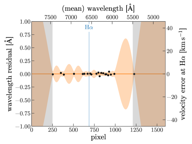
Typically, high-order standard polynomials or Chebyshev polynomials are used to fit for the wavelength dispersion function. We found that using such functions can lead to vastly incorrect wavelength values near either end of the pixel grid where the polynomial function is un- or weakly-constrained, and can easily over-fit to poorly centroided emission lines. We instead use a combined linear polynomial + GP to model the wavelength dispersion to flexibly account for nonlinear behavior in the pixel to wavelength mapping. We again use a Matérn 3/2 kernel, use L-BFGS-B optimization, and convert any scale parameter to log-space before maximizing the log-likelihood. Figure 9 shows an example of the residuals from one such fit; black points show the (pixel-centroid, wavelength) pairs with the best-fit model subtracted. The envelope around zero (shaded region, orange) shows the variance of the GP model projected into the data space; when the GP variance is large, the pixel-to-wavelength mapping is uncertain. We therefore only use the pixel range from 250–1210, corresponding to a wavelength range of $\approx 5500$–$7400~{}{\rm\AA}$; gray shaded region shows the excluded pixel/wavelength ranges.

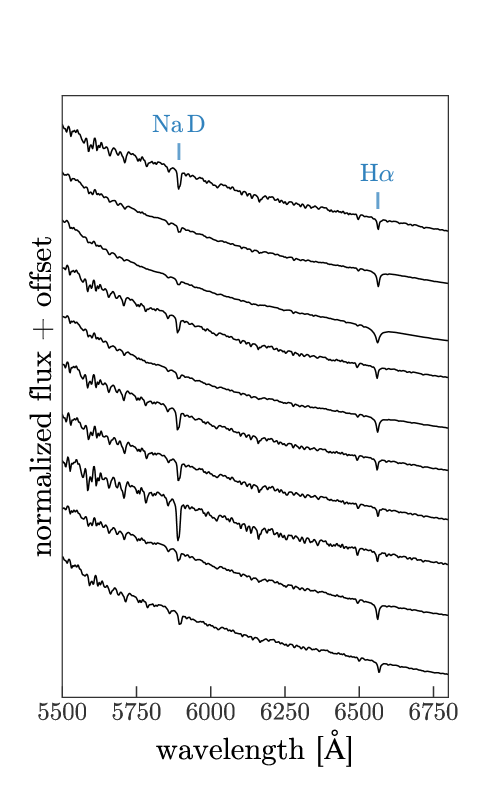
Figure 10 shows a random sample of 10 wavelength-calibrated source spectra of comoving star pair members normalized to 1 at $\lambda=5500~{}{\rm\AA}$ and shifted by an arbitrary offset for visualization. As suggested by the features (the number and depths of absorption features) in these 10 spectra, there is a mix of metallicities and spectral types amongst the observed targets. Note that the spectra are not flux-calibrated, as we only care about measuring radial velocities from this sample.

Figure 10: A section of 10 randomly selected target spectra from this work. Spectral fluxes are normalized to 1 at $\lambda=5500~{}{\rm\AA}$ and the offsets are chosen to separate the spectra for visualization. The spectra are smoothed with a Gaussian filter with root-variance $\sigma=2~{}{\rm\AA}$.

The wavelength calibration procedure described above produces a nightly model for the nonlinear dispersion of wavelength as a function of pixel value for each extracted 1D spectrum. However, because of flexure in the spectrograph, each observation will have an additional offset of, typically, $\approx 0.5$–$2~{}{\rm\AA}$, corresponding to a significant velocity offset at ${\rm H}\alpha$ of $\approx 25$–$100~{}\mathrm{km}~{}\mathrm{s}^{-1}$. As mentioned, comparison lamp spectra were not obtained at each telescope pointing. The absolute wavelength solution at each pointing can therefore be shifted (in pixels) relative to the nightly comparison lamp spectrum because of flexure in the instrument. We have found that this offset depends primarily on the hour angle of the observation, likely because of the physical orientation of the spectrograph and CCD as mounted on the telescope. To correct each source spectrum for this offset, we measure the centroids of the two prominent [OI] sky emission lines near $5577~{}{\rm\AA}$ and $6300~{}{\rm\AA}$ in the corresponding background spectrum derived from the spectral extraction (described above). We use a pixel-convolved Voigt profile as the emission line model (same parameters as above) and a Gaussian process with a Matérn 3/2 kernel function for the background spectrum (same parameters as above). We again use L-BFGS-B optimization and convert any scale parameter to log-space before maximizing the log-likelihood of this model to derive the line centroid in wavelength units. We compute wavelength offsets from true (air) values of the line centroids, $5577.3387~{}{\rm\AA}$ and $6300.304~{}{\rm\AA}$ respectively, then convert these wavelength offsets to pixel offsets. We take the mean of the pixel offsets and apply the derived shift to the source spectrum before re-computing the wavelength grid using the nightly wavelength solution. When one or both of the two sky lines is not present or the centroid fit fails, the spectrum is flagged as having a suspect wavelength calibration. In practice, most such sources are calibration targets, which are more likely to have very short exposure times and thus weak night-sky lines.

Parameter	Prior	Description
$\ln A$	$\mathcal{U}(2,16)$	Logarithm of line amplitude [${\rm photons}$]
$x_{0}$	$\mathcal{U}(6547,6579)$	Line wavelength centroid [${\rm\AA}$]
$\ln\sigma_{G}$	$\mathcal{U}(-4,2)$	Logarithm of Gaussian standard deviation of line profile [${\rm\AA}$]
$\ln\gamma_{L}$	$\mathcal{U}(-4,2)$	Logarithm of Lorentzian HWHM of line profile
$\alpha_{1}$	$\mathcal{U}(0,10^{16})$	Background model offset at line centroid [${\rm photons}$]
$\alpha_{2}$	$\mathcal{U}(-10^{8},10^{8})$	Background model slope [${\rm photons}~{}{\rm\AA}^{-1}$]
$\ln\sigma_{3/2}$	$\mathcal{U}(-8,8)$	Logarithm of Gaussian process amplitude [${\rm photons}$]
$\ln\rho_{3/2}$	$\mathcal{N}(1,1)$	Logarithm of Gaussian process correlation scale [${\rm\AA}$]

Table 2: Priors used for ${\rm H}\alpha$ line profile model parameters. $\mathcal{U}(a,b)$ indicates a uniform prior between $a$ and $b$ and $\mathcal{N}(\mu,\sigma^{2})$ indicates a normal distribution with mean $\mu$ and variance $\sigma^{2}$. Flux units are photons, i.e. the spectra are not flux-calibrated.

Appendix C Radial velocity measurement

To derive radial velocities for each source, we then measure the (wavelength) line centroid of ${\rm H}\alpha$ in each corrected spectrum. We model the absorption line using a pixel-convolved Voigt profile and use a linear model + a Gaussian process for the background model. We now use L-BFGS-B optimization and the resulting maximum-likelihood parameters to initialize a Markov Chain Monte Carlo (MCMC) sampling of the posterior probability distribution (PDF) over the 8 parameters: $\ln|A|$, $x_{0}$, $\ln\sigma_{G}$, $\ln\gamma_{L}$, $\alpha_{1}$, $\alpha_{2}$, $\ln\sigma_{3/2}$, and $\ln\rho_{3/2}$ where the linear background model is defined as $f(\lambda)=\alpha_{1}+\alpha_{2}\,\lambda$. The linear amplitude, $A$, is assumed to be negative (i.e. ${\rm H}\alpha$ is assumed to be an absorption feature) and is computed from the corresponding parameter as $A=-\exp(\ln|A|)$. We use uniform priors on all parameters except $\ln\rho_{3/2}$, for which we use a Gaussian; prior parameters are specified in Table 2. We use emcee (Foreman-Mackey et al. 2013a) with 64 walkers to generate samples from the posterior PDF. We initially run the sampler for 128 steps from the maximum likelihood parameter values, then resample walker positions in a small ball around the median final walker positions and run again for 512 steps; together, these two steps constitute our burn-in phase. From the final walker positions after burn-in, we run again for 1024 steps and store these as our posterior samples.

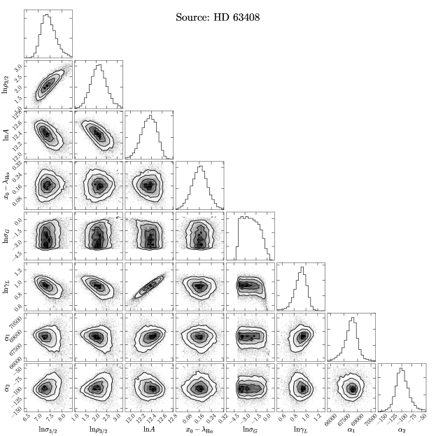
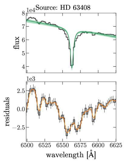
Figure 11 shows a corner plot of all projections of these posterior PDF samples for a randomly-chosen source (HD 63408, in this case). The marginal posterior distribution over $x_{0}$ can be converted to a distribution over radial velocity; in this case, the estimated (Gaussian standard deviation) precision is $\approx 2.5~{}\mathrm{km}~{}\mathrm{s}^{-1}$. Figure 12 shows the segment of the source spectrum around ${\rm H}\alpha$ used in the line modeling (black line) with uncertainties (gray bars). Top panel shows the linear polynomial + absorption line model computed for the median sample (dark green line); shaded region shows the 15th to 85th percentiles computed from all posterior samples. Bottom panel shows the residuals of the data from the median linear polynomial + absorption line model (black line) along with the Gaussian process computed from the median parameters (orange curve) used to model other correlated structure in the vicinity of ${\rm H}\alpha$ (which can be interpreted as correlated noise). These figures are produced for all source spectrum fits and visually inspected to ensure that the MCMC sampling appears to have converged for all cases.

For each source spectrum, with the resulting posterior samples, we compute the median and median absolute deviation (MAD) of the marginal distribution over line centroid, $x_{0}$. We use the MAD to estimate the standard deviation ($\sigma\approx 1.5\times{\rm MAD}$, assuming the samples are Gaussian distributed) of the samples and find that the typical velocity precision from measuring the centroid of ${\rm H}\alpha$ is between $5$–$10~{}\mathrm{km}~{}\mathrm{s}^{-1}$. We report the measured absolute radial velocities along with compiled sky position, astrometry, and $G$-band magnitude from the TGAS catalog and 2MASS $J$-band magnitudes for all of our comoving star targets in Table 3 available with this Article (see table caption for a detailed description of the contents).

Figure 11: A corner plot showing all projections of posterior PDF samples for the ${\rm H}\alpha$ line model and the spectrum of the source HD 63408. Note the small uncertainty in the line centroid measurement, $x_{0}$, which corresponds to a $\approx 2~{}\mathrm{km}~{}\mathrm{s}^{-1}$ velocity precision for this source. Parameters are described in Section 2.2, and prior PDFs over the parameters are described in Table 2.

Figure 12: Visualization of the ${\rm H}\alpha$ absorption line model and fits for the source HD 63408 as a demonstration of the procedure used for all targets. Top: The source spectrum in a small wavelength range around ${\rm H}\alpha$ (black), uncertainty in spectral flux (gray error bars). Over-plotted is the line model + background computed from the median posterior PDF sample (dark green line) and the 15th to 85th percentile region computed from all posterior PDF samples (shaded green region). Bottom: Source spectrum residuals computed by subtracting the median model (dark green line in top panel) from the source spectrum. The over-plotted line (orange) shows the Gaussian process background model computed from the median posterior PDF sample.

Appendix D Data products

See tables below for full descriptions of the columns in the associated data files.

Table 3: Description of columns in data table containing absolute radial velocity measurements and summary information from the TGAS catalog.

Column Name	Unit	Description
Oh17_group_id		Group ID from the candidate catalog (Oh et al. 2017)
tgas_source_id		Unique source identifier from TGAS
name		HD, Hipparcos, or Tycho-2 identifier
ra	deg	Right ascension from TGAS
dec	deg	Declination from TGAS
parallax	mas	Parallax from TGAS
distance	pc	Distance estimate using inverse parallax from TGAS
G	mag	Gaia $G$-band magnitudes
J	mag	2MASS $J$-band magnitudes
rv	$\mathrm{km}~{}\mathrm{s}^{-1}$	Radial velocity measured in this work
rv_err	$\mathrm{km}~{}\mathrm{s}^{-1}$	Radial velocity error

Table 4: Description of columns in data table containing separations and relative radial velocities for all observed groups, along with likelihood ratios computed with and without relative radial velocities.

Column Name	Unit	Description
Oh17_group_id		Group ID from candidate catalog (Oh et al. 2017)
R_mu		Log-likelihood-ratio computed with only astrometric information
R_rv		Log-likelihood-ratio computed with radial velocities as well
sep_tan	$\mathrm{pc}$	Median of tangential separation error distribution
sep_tan_err	$\mathrm{pc}$	Uncertainty in tangential separation
relative_rv	$\mathrm{km}~{}\mathrm{s}^{-1}$	Relative radial velocity between the two stars
relative_rv_err	$\mathrm{km}~{}\mathrm{s}^{-1}$	Uncertainty in relative radial velocity

References

- Allen & Monroy-Rodríguez (2014) Allen, C., & Monroy-Rodríguez, M. A. 2014, ApJ, 790, 158
- Andrews et al. (2017) Andrews, J. J., Chanamé, J., & Agüeros, M. A. 2017, ArXiv e-prints, arXiv:1704.07829
- Astropy Collaboration et al. (2013) Astropy Collaboration, Robitaille, T. P., Tollerud, E. J., et al. 2013, A&A, 558, A33
- Bahcall et al. (1985) Bahcall, J. N., Hut, P., & Tremaine, S. 1985, ApJ, 290, 15
- Barbier-Brossat & Figon (2000) Barbier-Brossat, M., & Figon, P. 2000, A&AS, 142, 217
- Bensby et al. (2014) Bensby, T., Feltzing, S., & Oey, M. S. 2014, A&A, 562, A71
- Bovy (2017) Bovy, J. 2017, ArXiv e-prints, arXiv:1704.05063
- Brewer et al. (2016) Brewer, J. M., Fischer, D. A., Valenti, J. A., & Piskunov, N. 2016, ApJS, 225, 32
- Carrasco et al. (2016) Carrasco, J. M., Evans, D. W., Montegriffo, P., et al. 2016, A&A, 595, A7
- Chanamé (2007) Chanamé, J. 2007, in IAU Symposium, Vol. 240, Binary Stars as Critical Tools & Tests in Contemporary Astrophysics, ed. W. I. Hartkopf, P. Harmanec, & E. F. Guinan, 316–325
- Chanamé & Gould (2004) Chanamé, J., & Gould, A. 2004, ApJ, 601, 289
- Craig et al. (2015) Craig, M. W., Crawford, S. M., Deil, C., et al. 2015, ccdproc: CCD data reduction software, Astrophysics Source Code Library, , , ascl:1510.007
- Deng et al. (2012) Deng, L.-C., Newberg, H. J., Liu, C., et al. 2012, Research in Astronomy and Astrophysics, 12, 735
- Dotter et al. (2008) Dotter, A., Chaboyer, B., Jevremović, D., et al. 2008, ApJS, 178, 89
- ESA (1997) ESA, ed. 1997, ESA Special Publication, Vol. 1200, The HIPPARCOS and TYCHO catalogues. Astrometric and photometric star catalogues derived from the ESA HIPPARCOS Space Astrometry Mission
- Foreman-Mackey (2016) Foreman-Mackey, D. 2016, The Journal of Open Source Software, 1, doi:10.21105/joss.00024
- Foreman-Mackey et al. (2017) Foreman-Mackey, D., Agol, E., Angus, R., & Ambikasaran, S. 2017, ArXiv e-prints, arXiv:1703.09710
- Foreman-Mackey et al. (2013a) Foreman-Mackey, D., Hogg, D. W., Lang, D., & Goodman, J. 2013a, PASP, 125, 306
- Foreman-Mackey et al. (2013b) Foreman-Mackey, D., Conley, A., Meierjurgen Farr, W., et al. 2013b, emcee: The MCMC Hammer, Astrophysics Source Code Library, , , ascl:1303.002
- Gaia Collaboration et al. (2016a) Gaia Collaboration, Brown, A. G. A., Vallenari, A., et al. 2016a, A&A, 595, A2
- Gaia Collaboration et al. (2016b) Gaia Collaboration, Prusti, T., de Bruijne, J. H. J., et al. 2016b, A&A, 595, A1
- Ginsburg et al. (2016) Ginsburg, A., Parikh, M., Woillez, J., et al. 2016, astropy/astroquery: v0.3.4 release, , , doi:10.5281/zenodo.167867
- Gould & Chanamé (2004) Gould, A., & Chanamé, J. 2004, ApJS, 150, 455
- Høg et al. (2000) Høg, E., Fabricius, C., Makarov, V. V., et al. 2000, A&A, 355, L27
- Hunter (2007) Hunter, J. D. 2007, Computing In Science & Engineering, 9, 90
- Jiang & Tremaine (2010) Jiang, Y.-F., & Tremaine, S. 2010, MNRAS, 401, 977
- Kharchenko et al. (2007) Kharchenko, N. V., Scholz, R.-D., Piskunov, A. E., Röser, S., & Schilbach, E. 2007, Astronomische Nachrichten, 328, 889
- Kunder et al. (2017) Kunder, A., Kordopatis, G., Steinmetz, M., et al. 2017, AJ, 153, 75
- Leigh et al. (2016) Leigh, N. W. C., Stone, N. C., Geller, A. M., et al. 2016, MNRAS, 463, 3311
- Lépine & Bongiorno (2007) Lépine, S., & Bongiorno, B. 2007, AJ, 133, 889
- Lépine & Shara (2005) Lépine, S., & Shara, M. M. 2005, AJ, 129, 1483
- Lutz & Kelker (1973) Lutz, T. E., & Kelker, D. H. 1973, PASP, 85, 573
- Matérn (1986) Matérn, B. 1986, Spatial variation, Lecture notes in statistics (Springer-Verlag)
- Michalik et al. (2015) Michalik, D., Lindegren, L., & Hobbs, D. 2015, A&A, 574, A115
- Monroy-Rodríguez & Allen (2014) Monroy-Rodríguez, M. A., & Allen, C. 2014, ApJ, 790, 159
- Morton (2015) Morton, T. D. 2015, isochrones: Stellar model grid package, Astrophysics Source Code Library, , , ascl:1503.010
- Naoz & Fabrycky (2014) Naoz, S., & Fabrycky, D. C. 2014, ApJ, 793, 137
- Ness et al. (2015) Ness, M., Hogg, D. W., Rix, H.-W., Ho, A. Y. Q., & Zasowski, G. 2015, ApJ, 808, 16
- Nordström et al. (2004) Nordström, B., Mayor, M., Andersen, J., et al. 2004, A&A, 418, 989
- Oelkers et al. (2017) Oelkers, R. J., Stassun, K. G., & Dhital, S. 2017, AJ, 153, 259
- Oh et al. (2017) Oh, S., Price-Whelan, A. M., Hogg, D. W., Morton, T. D., & Spergel, D. N. 2017, AJ, 153, 257
- Oort (1950) Oort, J. H. 1950, Bull. Astron. Inst. Netherlands, 11, 91
- Öpik (1924) Öpik, E. 1924, Publications of the Tartu Astrofizica Observatory, 25
- Parker et al. (2009) Parker, R. J., Goodwin, S. P., Kroupa, P., & Kouwenhoven, M. B. N. 2009, MNRAS, 397, 1577
- Pérez & Granger (2007) Pérez, F., & Granger, B. E. 2007, Computing in Science and Engineering, 9, 21
- Pinsonneault et al. (2001) Pinsonneault, M. H., DePoy, D. L., & Coffee, M. 2001, ApJ, 556, L59
- Pinsonneault et al. (2014) Pinsonneault, M. H., Elsworth, Y., Epstein, C., et al. 2014, ApJS, 215, 19
- Quinn et al. (2009) Quinn, D. P., Wilkinson, M. I., Irwin, M. J., et al. 2009, MNRAS, 396, L11
- Raghavan et al. (2010) Raghavan, D., McAlister, H. A., Henry, T. J., et al. 2010, ApJS, 190, 1
- Rasmussen & Williams (2005) Rasmussen, C. E., & Williams, C. K. I. 2005, Gaussian Processes for Machine Learning (Adaptive Computation and Machine Learning) (The MIT Press)
- Reipurth & Mikkola (2012) Reipurth, B., & Mikkola, S. 2012, Nature, 492, 221
- Sesar et al. (2008) Sesar, B., Ivezić, Ž., & Jurić, M. 2008, ApJ, 689, 1244
- Shaya & Olling (2011) Shaya, E. J., & Olling, R. P. 2011, ApJS, 192, 2
- Skrutskie et al. (2006) Skrutskie, M. F., Cutri, R. M., Stiening, R., et al. 2006, AJ, 131, 1163
- Steinmetz et al. (2006) Steinmetz, M., Zwitter, T., Siebert, A., et al. 2006, AJ, 132, 1645
- Tokovinin & Lépine (2012) Tokovinin, A., & Lépine, S. 2012, AJ, 144, 102
- Torres (2013) Torres, G. 2013, in EAS Publications Series, Vol. 64, EAS Publications Series, ed. K. Pavlovski, A. Tkachenko, & G. Torres, 87–94
- Van der Walt et al. (2011) Van der Walt, S., Colbert, S. C., & Varoquaux, G. 2011, Computing in Science & Engineering, 13, 22
- Weinberg et al. (1987) Weinberg, M. D., Shapiro, S. L., & Wasserman, I. 1987, ApJ, 312, 367
- Wenger et al. (2000) Wenger, M., Ochsenbein, F., Egret, D., et al. 2000, A&AS, 143, 9
- Wright et al. (2010) Wright, E. L., Eisenhardt, P. R. M., Mainzer, A. K., et al. 2010, AJ, 140, 1868
- Yoo et al. (2004) Yoo, J., Chanamé, J., & Gould, A. 2004, ApJ, 601, 311
- Zhu et al. (1994) Zhu, C., Byrd, R. H., Lu, P., & Nocedal, J. 1994, L-BFGS-B - Fortran Subroutines for Large-Scale Bound Constrained Optimization, Tech. rep., ACM Trans. Math. Software