Stochastic Order Redshift Technique (SORT): a simple, efficient and robust method to improve cosmological redshift measurements

Abstract

We present a simple, efficient and robust approach to improve cosmological redshift measurements. The method is based on the presence of a reference sample for which a precise redshift number distribution ($dN/dz$) can be obtained for different pencil-beam-like sub-volumes within the original survey. For each sub-volume we then impose: (i) that the redshift number distribution of the uncertain redshift measurements matches the reference $dN/dz$ corrected by their selection functions; and (ii) the rank order in redshift of the original ensemble of uncertain measurements is preserved. The latter step is motivated by the fact that random variables drawn from Gaussian probability density functions (PDFs) of different means and arbitrarily large standard deviations satisfy stochastic ordering. We then repeat this simple algorithm for multiple arbitrary pencil-beam-like overlapping sub-volumes; in this manner, each uncertain measurement has multiple (non-independent) “recovered” redshifts which can be used to estimate a new redshift PDF. We refer to this method as the Stochastic Order Redshift Technique (sort). We have used a state-of-the art $N$-body simulation to test the performance of sort under simple assumptions and found that it can improve the quality of cosmological redshifts in an robust and efficient manner. Particularly, sort redshifts ($z_{\rm sort}$) are able to recover the distinctive features of the so-called ‘cosmic web’ and can provide unbiased measurement of the two-point correlation function on scales $\gtrsim 4$ $h^{-1}$Mpc. Given its simplicity, we envision that a method like sort can be incorporated into more sophisticated algorithms aimed to exploit the full potential of large extragalactic photometric surveys.

1 Introduction

Observational constraints of the galaxy distribution are of fundamental importance for cosmology and astrophysics. As tracers of the underlying matter distribution, the actual three-dimensional positions of galaxies contain relevant information regarding the initial conditions of the Universe, cosmological parameters, and the nature of dark matter and dark energy (e.g. Plionis & Basilakos, 2002; Cole et al., 2005; Li, 2011; Bos et al., 2012; Gillet et al., 2015; Cai et al., 2015). This so-called ‘cosmic web’ also affects the physical condition of the bulk of baryonic matter residing in the intergalactic medium (e.g. Cen & Ostriker, 1999; Davé et al., 2001; Shull et al., 2012), which in turn could also shape the evolution of galaxies themselves (e.g. Mo et al., 2005; Peng et al., 2010; Lu et al., 2015; Peng et al., 2015; Aragon-Calvo et al., 2016).

Of particular interest is to resolve the cosmic web and the density distribution on scales $\lesssim 1-10$ $h^{-1}$Mpc, where the clustering power of matter is larger. At these scales, galaxies form an intricate network of filaments, sheets and nodes, while also leaving vast volumes virtually devoid of luminous matter (i.e. galaxy voids). In order to access the rich information provided by these complex patterns, one must survey galaxies with redshift precision comparable or smaller than such scales.

State-of-the-art photometric redshifts can achieve redshift precisions of $\sigma_{z}^{\rm ph}\approx 0.02$ (e.g. for SDSS at $z<0.6$, Beck et al., 2016, and references therein), which correspond to scales of $\sim 70$ $h^{-1}$Mpc at $z\sim 0.5$. This is essentially about an order of magnitude larger than the precision needed to resolve most of the cosmic web patterns. This precision is unlikely to improve drastically over the next decade; the photometric redshift technique usually relies on fitting spectral energy distributions (SEDs) using a fixed set of relatively broad band filters. Thus, despite having access to deeper observations, more realistic SED templates, better characterization of systematics, and/or more complex fitting algorithms, it is the widths of the photometric filters that determine the intrinsic limit precision of such techniques. Even photometric surveys that use a comparatively large number of contiguous medium band filters (e.g. ALHAMBRA; Arnalte-Mur et al., 2014) do not seem to significantly improve over a $\sigma_{z}^{\rm ph}\approx 0.02$.

In such an scenario, it seems inevitable to rely (at least partially) on precise spectroscopic redshifts. As opposed to broad band filters, the spectroscopic redshift estimations come from resolving spectral features (usually narrow; e.g. emission/absorption lines, continuum breaks, etc.), providing redshift precisions mostly limited by the resolution of the spectrograph. Even low-resolution ($R\equiv\frac{\lambda}{\Delta\lambda}\approx 200$) spectroscopy can easily reach $\sim 1$ $h^{-1}$Mpc scale precision. However, spectroscopic redshifts are comparatively more expensive due to the combination of reduced sensitivity, spectral coverage, and field-of-view coverage.

Due to these limitations, it is sensible to adopt an hybrid approach, where the precise redshift estimations (e.g. spectroscopic) of a small subsample of the survey are used to improve the less precise cosmological redshift measurements (e.g. photometric) of the majority of the targets in the survey. This is in principle possible assuming that most of the luminous galaxies occupy relatively small volumes. In such a case, small reference samples could still provide a sensible mapping of large-scale structures which can be used to better constrain the positions along the line-of-sight of relatively close neighbours.

The idea of using spectroscopic samples to empirically improve the redshift distribution of photometric samples is not new (e.g., Padmanabhan et al., 2005; Sheth, 2007; Lima et al., 2008; Cunha et al., 2009). In general, these studies focus on improving the underlying redshift distribution of a photometric sample rather than individual galaxy redshifts; thus, those methods are appropriate for applications where the individual information of galaxies is not required. Some examples of these include surveys aimed at studying Baryonic Acoustic Oscillations (BAOs), weak lensing, growth of density perturbations, dark energy from galaxy distributions and the integrated Sachs-Wolf effect.

Alternative methods exist for improving the individual photometric redshift of galaxies. For example, the method developed in Aragon-Calvo et al. (2015) uses the information of the cosmic web itself to find the maximum likelihood locations of individual photometric galaxies to the nearest cosmic web ‘element’. Another approach is to use the spatial clustering of galaxies (e.g. Phillipps & Shanks, 1987; Landy et al., 1996; McQuinn & White, 2013; Ménard et al., 2013). These methods use the information of both the redshift distribution and angular clustering of a spectroscopic reference sample to improve the individual redshifts of a photometric sample. Particularly, the implementation presented by Ménard et al. (2013) has been recently successfully applied to the the Two-Micron All-Sky Survey (2MASS) and the Sloan Digital Sky Server (SDSS) (Rahman et al., 2016a, b). The virtue of these methods is that they can provide a redshift measurement that is essentially independent of the photometric redshift based on SEDs, thus both probability density distributions (PDFs) can be multiplied to infer an improved redshift measurement for individual sources. Unfortunately, none of these methods are easily accessible to the community and also these tend to be computationally expensive. Another limitation is that they usually rely on wide field surveys and it is not straightforward how to apply them to much narrower geometries (particularly pencil-beam-like ones).

This paper presents a very simple and complementary method to improve cosmological redshift measurements obtained on surveys with arbitrary geometries. Broadly speaking, the method considers a patch on the sky where initially two kinds of redshift measurement exist: uncertain (e.g. photometric) and precise (e.g. spectroscopic). The ones with precise redshifts will be used as a ‘reference sample’ and it is of course is expected that these correspond to a small fraction of the total number of objects. We then rank order both distributions in order to find a correlation between the reference and the uncertain sample. As we will show later, this idea is motivated by the fact that random variables drawn from Gaussian PDFs of different means and arbitrarily large standard deviations satisfy stochastic ordering. We thus refer to this method as the Stochastic Order Redshift Technique (sort).

By construction, sort is non-parametric as it does not need to assume any functional form for either the distribution of redshift or the relationship between spectroscopic and photometric redshifts. Thus, the power of sort relies on its simplicity and versatility. We show that sort is indeed robust and that it can provide unbiased measurement of the redshift-space two-point correlation function on scales $\gtrsim 4$ $h^{-1}$Mpc, while also recovering the distinctive features of the cosmic web (voids, filaments, clusters). Given its simplicity, we expect that a method like sort could be incorporated into more sophisticated algorithms aimed to improve cosmological redshifts in order to fully exploit the potential of large extragalactic photometric surveys like the Dark Energy Survey (DES; Flaugher, 2012; Dark Energy Survey Collaboration et al., 2016) or the The Large Synoptic Survey Telescope (LSST Science Collaboration et al., 2009). Moreover, because sort can be applied to both wide and narrow surveys, we also expect to be suitable for current surveys like COSMOS (Scoville et al., 2007; Koekemoer et al., 2007) or CANDELS (Grogin et al., 2011; Koekemoer et al., 2011).

This paper is organized as follows. In Section 2, we describe the method, while in Section 3 we describe the galaxy survey used to study its performance. In Section 4 we present the results of applying sort to our mock galaxy survey, including redshift PDFs, two-point correlation functions and inferred three-dimensional distributions of galaxies. In Section 5 we provide a discussion regarding information content, efficiency, versatility, limitations, and a comparison to other methods. Section 6 presents a summary and main conclusions.

2 The method

We propose a simple and efficient method to improve cosmological redshift measurements whose uncertainties are larger than that of the intrinsic ‘cosmic web’ scales. The general idea behind the method is based on the use of a reference sample and stochastic order as we describe below.

2.1 General considerations

Figure 1: An illustration of our method based on stochastic order. Step (A): In a given pencil-beam-like sub-volume we define two samples of extragalactic objects depending on the accuracy of their cosmological redshift determination: precise (e.g. spectroscopic; left panels) and uncertain (e.g. photometric; right panels). Step (B): From both samples we observe a redshift number density, $dN/dz$. In principle, the uncertain $dN/dz$ (left panel) is a nosier version of the precise one (right panel). Step (C): From the precise distribution we create a new re-sampled redshift distribution matching the number of objects in the uncertain sample (left panel) and sort it from low to high redshift. We also sort the observed uncertain redshift distribution from low to high redshift (right panel). Step (D): Finally, we perform a one-to-one match between the recovered distribution in the left and right panels of step (C). We refer to this simple algorithm as Stochastic Ordering Redshift Technique (sort).

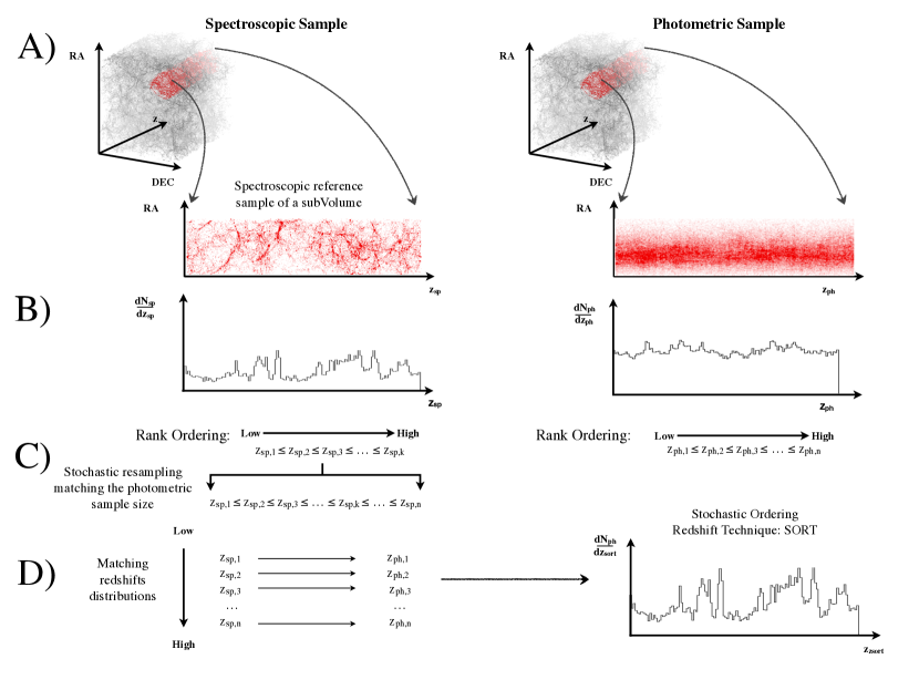
Let us consider a survey of $N_{\rm tot}$ galaxies in a volume $V$. Suppose that in this galaxy survey we find that for a number of $N_{\rm ph}$ galaxies the quality of their individual redshifts is poor (hereafter referred to as the photometric sample), and that $N_{\rm sp}$ galaxies have a reliable redshift estimation (referred to as the spectroscopic sample). The upper row of Figure 1 illustrates the situation described above. It is evident that the probability redshift distributions of these two subsamples are different: while the spectroscopic sample traces a complex distribution, such information is somewhat lost in the photometric sample (see B row of Figure 1). Observationally, one can constrain these probability distributions, $P(z)$, by means of their redshift number density, $dN/dz(z)$, i.e. the number of galaxies per unit redshift in a given sample. Thus,

$$P_{\rm ph}(z_{\rm ph})=\frac{1}{S_{\rm ph}}\frac{1}{N_{\rm ph}}\frac{dN_{\rm ph}}{dz_{\rm ph}}(z_{\rm ph})$$ (1)

and,

$$P_{\rm sp}(z_{\rm sp})=\frac{1}{S_{\rm sp}}\frac{1}{N_{\rm sp}}\frac{dN_{\rm sp}}{dz_{\rm sp}}(z_{\rm sp})$$ (2)

where $S_{\rm ph}$ and $S_{\rm sp}$ are the selection functions for these two samples, respectively. The selection function should depend on redshift, but it can also depend on position on the sky and any other property of the extragalactic object (e.g. luminosity, morphology, star-formation rate, etc.). Assuming that there is a real redshift probability distribution traced by galaxies, these distributions can also be written as

$$P_{\rm ph}(z_{\rm ph})=\int\mathcal{R}_{\rm ph}(z-z_{\rm ph})P_{\rm real}(z)\,dz$$ (3)

and,

$$P_{\rm sp}(z_{\rm sp})=\int\mathcal{R}_{\rm sp}(z-z_{\rm sp})P_{\rm real}(z)\,dz$$ (4)

where $\mathcal{R}_{\rm ph}$ and $\mathcal{R}_{\rm sp}$ are the redshift uncertainties of the photometric and spectroscopic samples, respectively. The redshift resolution of these estimations are therefore limited by the redshift uncertainties of the galaxies in their respective samples (see panel B of Figure 1 for an illustration); one can consider $P_{\rm ph}$ be a noisier version of $P_{\rm sp}$.

Assuming that the subsample of $N_{\rm sp}$ galaxies with spectroscopic redshifts is ‘statistically relevant’—i.e. that they accurately trace the underlying cosmic structures such as clusters, filaments, walls and voids present in the volume $V$— this naturally suggests that the spectroscopic subsample can be used to improve the quality of the redshift distribution of the photometric sample. In other words, we can assume that the probability redshift distribution of the photometric sample, $P_{\rm ph}$, is the probability redshift distribution of the spectroscopic sample, $P_{\rm sp}$, convolved with an unknown kernel $\mathcal{G}$,

$$P_{\rm ph}(z_{\rm ph})=\int\mathcal{G}(z_{\rm ph}-z_{\rm sp})P_{\rm sp}(z_{\rm sp})dz_{\rm sp}$$ (5)

Therefore, the problem of improving photometric redshift estimations may reduce to constrain all the moments of $\mathcal{G}$, particularly its mean relation (i.e. $z_{\rm ph}-z_{\rm sp}$) and the dispersion around the mean. The general approach has been then to constrain $\mathcal{G}$ and use Equation 5 to improve the redshift estimations of the photometric sample.

In this paper we propose a complementary approach, in which we do not constrain $\mathcal{G}$ itself to obtain the underlying $P(z)$, but use the overall relation between their cumulative distributions instead. Let us consider the simple case when the correlation between $z_{\rm sp}$ and $z_{\rm ph}$ is a one-to-one monotonic relation with zero scatter, i.e. $\mathcal{G}(z_{\rm ph}-z_{\rm sp})$ becomes the Dirac delta function. Then Equation 5 can be written as:

$$\frac{dN_{\rm ph}}{dz_{\rm ph}}(z_{\rm ph})=\frac{N_{\rm ph}}{N_{\rm sp}}\frac{S_{\rm ph}}{S_{\rm sp}}\frac{dN_{\rm sp}}{dz_{\rm sp}}(z_{\rm sp}(z_{\rm ph}))\frac{dz_{\rm sp}}{dz_{\rm ph}},$$ (6)

where we use the definitions of Equations 1 and 2. The above Equation can be written in terms of the following integrals:

$$\int_{z_{\rm ph}}^{\infty}\frac{dN_{\rm ph}}{dz^{\prime}_{\rm ph}}dz^{\prime}_{\rm ph}=\frac{N_{\rm ph}}{N_{\rm sp}}\int_{z_{\rm sp}}^{\infty}\frac{S_{\rm ph}}{S_{\rm sp}}\frac{dN_{\rm sp}}{dz^{\prime}_{\rm sp}}dz^{\prime}_{\rm sp}.$$ (7)

An easy way to solve Equation 7 is just rank ordering spectroscopic galaxies by their redshift and assigning them to photometric galaxies also ranked by redshift (see bottom panel of Figure 1 and Equation 8 below). Obviously, in the presence of scatter in the relation $\mathcal{G}$ this solution is not strictly valid but just an approximation. In this paper, we explore how good such an approximation is, and show that it is indeed suitable for improving photometric redshifts.

2.2 Stochastic Order Redshift Technique (SORT)

We solve Equation 7 by sorting the $N_{\rm ph}$ observed photometric redshifts such that $z_{1}^{\rm obs}\leq z_{2}^{\rm obs}\leq\dots\leq z_{N_{\rm ph}}^{\rm obs}$, and assign them $N_{\rm ph}$ sorted recovered redshifts, randomly sampled from,

$$\frac{N_{\rm ph}}{N_{\rm sp}}\frac{S_{\rm ph}}{S_{\rm sp}}\frac{dN_{\rm sp}}{dz}(z)\to\{z_{1}^{\rm rec},z_{2}^{\rm rec},\dots,z_{N_{\rm ph}}^{\rm rec}\}$$ (8)

such that $z_{1}^{\rm rec}\leq z_{2}^{\rm rec}\leq\dots\leq z_{N_{\rm ph}}^{\rm rec}$. This provides a straightforward one-to-one mapping between the observed and recovered photometric redshift distributions as $z_{i}^{\rm obs}\leftrightarrow z_{i}^{\rm rec}$, for $i\in\{1,2,\dots,N_{\rm ph}\}$ (see bottom panel of Figure 1). This is a simplistic but powerful approach, particularly because photometric samples are expected to satisfy stochastic ordering.

We define stochastic order as follows. Consider two random variables, $X_{i}$ and $X_{j}$, being drawn from two arbitrary probability density functions (PDFs), $P_{i}$ and $P_{j}$ in the domain $x$. Then, we say that $X_{j}$ is stochastically greater than or equal to $X_{i}$ if and only if their PDFs satisfy,

$$P_{i}(X_{i}>x)\leq P_{j}(X_{j}>x)\ \ \ \forall x\ \ \rm{,}$$ (9)

(e.g. Shaked & Shanthikumar, 2007). This is equivalent to saying that,

$$\int_{x}^{\infty}P_{i}(x^{\prime})\,dx^{\prime}\leq\int_{x}^{\infty}P_{j}(x^{\prime})\,dx^{\prime}\ \ \ \forall x\ \ \rm{.}$$ (10)

Let us now consider the case of individual redshift estimations, $z_{i}$ and $z_{j}$, whose PDFs are given by Gaussians having the same (arbitrarily large) standard deviations, centred at $z_{i}$ and $z_{j}$, respectively, and satisfying $z_{i}<z_{j}$. If we treat these redshift measurements as random variables, it is straightforward to show that stochastic order is satisfied (Equation 9 or Equation 10). Hence, even though their PDFs may overlap in redshift, the most likely outcome is having $z^{\rm true}_{i}\leq z^{\rm true}_{j}$, where $z^{\rm true}_{\{i,j\}}$ are their true underlying redshifts, respectively.

Stochastic order ensures transitivity, meaning that independently of the individual photometric redshift uncertainties, their observed rank order within the sample most likely matches that of the underlying true values. Thus, by solving Equation 7 using Equation 8 this information is also preserved.

Although there may be cases where Equation 9 does not apply (e.g. complex PDFs with asymmetries or multiple local maxima), we can expect that state-of-the-art photometric redshift estimations provide well behaved PDFs, where stochastic order is satisfied for a significant fraction of the photometric sample. Under this assumption, we thus refer to this matching scheme as the Stochastic Order Redshift Technique (sort).

We emphasize that sort is a statistical method and should be only applied to ensembles rather than individual measurements. We also note that this simplistic version of sort could eventually lead to catastrophic redshifts, i.e. $z_{i}^{\rm rec}$ that are not statistically consistent with the $z_{i}^{\rm obs}$ individual PDFs. Indeed, this is the case because in its current implementation we are not using the information provided by the individual photometric uncertainties. We chose this approach so we can explore the advantages/disadvantages of the method in its simplest form (but see Section 5.1 for how to easily prevent catastrophic redshift assignments).

In the following we test sort using a mock galaxy survey drawn from a state-of-the-art $N$-body cosmological simulation aimed at reproducing the low-$z$ ($z\lesssim 0.3$) SDSS. We emphasize that even though we will mainly refer to a galaxy survey, in practice we can apply this method to any kind of luminous extragalactic object.

3 Simulation

In order to test the performance of sort we create a magnitude-limited mock galaxy survey on the $N$-body MultiDark-Planck simulation (Klypin et al., 2016). The MultiDark-Planck simulation is a very high resolution simulation based on a $\Lambda$CDM cosmology with the results from the Planck Collaboration (Planck Collaboration et al., 2016): $\Omega_{\rm M}=0.307$, $\Omega_{\Lambda}=1-\Omega_{\rm M}$, $\Omega_{\rm B}=0.048$, $\sigma_{8}=0.829$, $n_{s}=0.96$ and $h=0.678$. The length of the simulation is $1$ $h^{-1}$Gpc per side and it contains $3840^{3}$ particles of mass $m_{\rm p}=1.5\times 10^{9}$  $h^{-1}M_{\odot}$.

3.1 Mock galaxy survey

We created a mock magnitude limited galaxy survey based on the MultiDark Planck simulation (Klypin et al., 2016; Rodríguez-Puebla et al., 2016). Dark matter haloes and subhalos were identified using the Rockstar phase-space temporal halo finder (Behroozi et al., 2013). Halo mass is defined using the virial overdensity given by the spherical collapse model which corresponds to $\Delta=333$ at $z=0$ for our adopted cosmology. We then imposed a minimum halo mass of $10^{12}h^{-1}$$M_{\odot}$, and assume that each one of those haloes/subhaloes will host a luminous galaxy. Galaxies were assigned via abundance matching (Vale & Ostriker, 2004) by using the luminosity function of the SDSS DR7 (Yang et al., 2009) in the $r$-band that will be denoted simply as $M$.

We placed a virtual observer at one of the corners of the simulated box and projected each galaxy position in co-moving Cartesian coordinates into Spherical Coordinates assuming the pole to be aligned with one of the Cartesian axes. In this manner, the simulated box is projected into a single spherical octant. We assign the azimuthal angle to the so-called right ascension of the Celestial Coordinates (RA), and the complement of the polar angle to the so-called declination of the Celestial Coordinates (Dec.). We used the total co-moving distance of each galaxy to the position of the virtual observer to define cosmological redshifts, $z_{\rm cos}$, from our adopted cosmology.

Apparent magnitudes, $m$, were obtained from

$$m=M+\mu(z_{\rm cos})$$ (11)

where $\mu(z)$ is the distance modulus as a function of redshift. We imposed a maximum apparent magnitude limit in the $r$-band of $m^{\rm max}_{r}=18.5$ mag. This criterion led to $127\,993$ galaxies, all at cosmological distances smaller than the size of the simulation box.

We define ‘true’ redshift, $z_{\rm true}$, from

$$1+z_{\rm true}=(1+z_{\rm cos})(1+\frac{\Delta v_{\rm los}}{c})\ \rm{,}$$ (12)

where $\Delta v_{\rm los}$ is the simulated velocity component along the line-of-sight (i.e. peculiar velocity), and $c$ is the speed of light. This $z_{\rm true}$ will be considered the intrinsic true value of an individual galaxy’s redshift. In order to simulate an observed redshift, we added noise in the form of

$$z_{\rm obs}=z_{\rm true}+\delta_{z}(1+z_{\rm true})\ \rm{,}$$ (13)

where $\delta_{z}$ is a value randomly sampled from a Gaussian distribution centred at zero with standard deviation $\sigma_{z}$.

3.2 Galaxy subsamples

We define two main subsamples of galaxies based on two different level of noise applied to their $z_{\rm true}$ (see Equation 13),

• The photometric sample: defined by using a $\sigma_{z}^{\rm ph}=0.02$ encompassing $70\%$ of the magnitude limited sample (randomly chosen).

• The spectroscopic sample: defined by using $\sigma_{z}^{\rm sp}=0.0001$ for the remaining $30\%$ of the sample.

We chose $\sigma_{z}^{\rm ph}=0.02$ as a representative state-of-the-art photometric precision (this is also comparable to the goal of the future Large Synoptic Survey Telescope, LSST). The $30\%$ reference fraction was chosen as representative of current large extragalactic surveys at our chosen magnitude limit (e.g. SDSS). For simplicity, in the following we restrict the analysis to a unique sample using these fiducial values. For a discussion on the performance of the method using lower fractions of spectroscopic galaxies and larger photometric uncertainties we refer the reader to Section 5.2.

Figure 2: Redshift distributions (arbitrary binning of $0.0015$) for our photometric mock galaxy survey for different redshifts: photometric ($z_{\rm ph}$; red histograms), sort ($z_{\rm sort}$; black histograms) and true ($z_{\rm true}$; grey histograms). The top panel shows the full photometric sample, while the middle and bottom panels split the mock survey to roughly the half-bright and half-faint subsamples, respectively, by using a $m=18$ limit. See Section 4.2 for further details.

Figure 3: Two-dimensional normalized histograms (arbitrary binning $0.0015$) for the original photometric redshift ($z_{\rm ph}$; left panel $y$-axis) and that of sort ($z_{\rm sort}$; right panel $y$-axis), both as a function of the underlying true redshift ($z_{\rm true}$; $x$-axes). The grey scale is linearly proportional to the number of counts in each normalized bin and the contours mark the limits where the counts are multiples of $1/4$ the maximum value. See Section 4.3 for further details.

4 Results

In this section we describe our sort method applied to the mock galaxy survey described in the previous section. We will assume that $30\%$ of our final sample of 127993 galaxies have spectroscopic redshifts. In reality, this fraction is a free parameter however. We refer the reader to Section 5.2 where we explore the performance of the method with different choices.

4.1 Applying the method

1. For each individual galaxy with apparent magnitude $m$, we define a projected area $A$ as a circle of angular radius $R$.

2. We then consider only galaxies in $A$ having apparent magnitudes within $\Delta m$ from $m$.

3. From these galaxies, we check that at least $N^{\rm ref}_{\rm min}$ have spectroscopic redshifts. Otherwise, we iterate steps (i) and (ii) increasing the values of $R$ and $\Delta m$ by $\delta R$ and $\delta m$, respectively, until the condition is satisfied.

4. We compute a redshift histogram of the $N^{\rm ref}$ galaxies using redshift bins of width $\delta z/3$. We then convolve this histogram with a Gaussian kernel of standard deviation $\delta z$, and use the resulting distribution to randomly sample $N^{\rm rec}_{\rm ph}$ redshifts, where $N^{\rm rec}_{\rm ph}$ is the number of photometric galaxies within $A$.

5. We apply the stochastic order matching scheme described in Section 2.2 (see Equation 8) to obtain recovered redshifts for each individual photometric galaxy.

We repeated this algorithm for all the photometric galaxies in the sample. In this manner, each photometric galaxy has a list of recovered redshifts, each one coming from an independent random sampling of their respective reference (spectroscopic) sample. This is equivalent to having adaptive Monte Carlo realizations, as galaxies in denser regions will be sampled more times than galaxies in less dense regions. For simplicity, we finally take the median value of the aforementioned recovered distribution list as the actual unique recovered sort redshift, $z_{\rm sort}$.

For the results of this paper we applied the aforementioned algorithm using the following parameters: $R=1$ degree, $\Delta m=0.2$ mag, $\delta R=0.1$ degree, $\delta m=0.1$ mag, $N^{\rm ref}_{\rm min}=2$ and $\delta z=0.0003$. By choosing $N^{\rm ref}_{\rm min}=2$ we make sure that for each iteration there are at least $2$ galaxies with a spectroscopic redshift measurement as reference. Because of our survey is magnitude limited, for the brightest galaxies this condition means that the radius of the search ends up being larger than the fiducial value $R=1$ degree, up to a factor of $\approx 1.5-2.5\times$ for those with magnitudes $m\sim 15-14$ mag respectively. The fraction of bright galaxies is very small and we do not consider this issue to be a major limitation of our method; in any case, the brightest objects are the cheapest to get a spectroscopic redshift for, hence making it feasible to eventually correct for this in the future.

We have chosen a relatively small $\Delta m=0.2$ mag in order to ensure a similar selection function for galaxies for the photometric and spectroscopic samples as a function of $m$. In this manner we avoid introducing shot noise from correcting for the different selection functions with a sparse sampling.

Figure 4: Normalized distribution (arbitrary binning of $0.0005$) of the redshift differences with respect to the true redshift $z_{\rm true}$, for both the original photometric redshifts ($z_{\rm ph}$, red histogram), and those from our sort method ($z_{\rm sort}$, black histogram). See Section 4.3 for further details.

Figure 5: Mean redshift difference with respect to the true underlying value, $\Delta z\equiv z-z_{\rm true}$ using the original photometric redshifts ($z=z_{\rm ph}$; left panel, red squares) and sort redshifts ($z=z_{\rm sort}$; right panel, black circles) both as a function of the used redshift $z$ (arbitrary binning of $0.015$). We also show the underlying distributions as normalized two-dimensional histograms with the same binning and contour scheme as Figure 3. See Section 4.3 for further details.

Although the area $A$ can in principle have any arbitrary shape, we have chosen a circular one only for simplicity. We note that $1$ degree corresponds to $\approx 5-10$ $h^{-1}$Mpc at redshifts $z\approx 0.06-0.12$ (where most of our mock galaxies reside). We chose a $\delta z=0.0003$ which is $3\times$ our adopted $\sigma_{z}^{\rm sp}$, corresponding to $\approx 1$ $h^{-1}$Mpc (if cosmological) along the line-of-sight at these redshifts. Therefore, our chosen $R$ and $\delta z$ will capture the most relevant scales of the cosmic web traced by luminous galaxies. We emphasize that our method is very general, and by construction it only ensures that the overall $P_{\rm gal}(z)$ distributions between the photometric and spectroscopic samples are statistically consistent with each other (when corrected for their respective selection functions). However, by choosing a scale comparable to the cosmic web we also expect to perform relatively well at recovering the three-dimensional distribution of galaxies (see Section 4.3.1) and the two-point auto-correlation function on scales $\gtrsim 5$ $h^{-1}$Mpc (see Section 4.3.2).

4.2 Redshift distributions

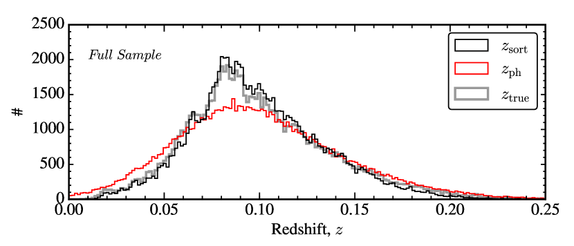
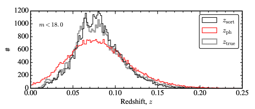
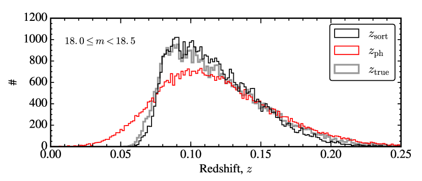
In Figure 2 we plot the redshift distributions of the mock galaxies using our different samples: photometric ($z_{\rm ph}$; red histograms), sort ($z_{\rm sort}$; black histograms) and true ($z_{\rm true}$; grey histograms). The top panel shows the full sample, while the middle and bottom panels split the mock survey to roughly the half-bright and half-faint subsamples, respectively, by using a $m=18$ limit. As expected, the photometric uncertainties are large enough to ‘wash out’ most of the large-scale structure information, resulting in smooth distributions at virtually all relevant scales. In contrast, the $z_{\rm sort}$ distributions match the true distributions better than the photometric redshifts, not just in the overall shape (given mostly by the selection function), but also the fluctuations induced by the large-scale structure of the cosmic web itself (i.e. peaks and valleys). This match is not perfect however, as one can observe that some large-scale structures are somewhat over/under represented. These discrepancies mainly come from the sparse sampling of spectroscopic galaxies used as reference at the low and high ends of the distribution (more evident at $z<0.05$), which for conservation of the total numbers introduce an oversampling at intermediate redshifts (e.g. those at $z\approx 0.09-0.1$). These discrepancies are small enough that they do not produce any noticeable bias in the most relevant statistical quantities that we have explored (see next sections). We note that one could in principle compensate for this by modifying the selection functions used in the method, for which a mock galaxy survey will be needed for adequate calibration. However, because in this paper focuses on the simplicity of the method, in the following we do not introduce any such fine-tuning compensation.

Figure 6: A declination slice (arbitrary thickness of $5$ degrees) of the three-dimensional distribution of our mock galaxy survey, using different redshift measurements: original photometric ($z_{\rm ph}$; top left), original spectroscopic used as reference ($z_{\rm sp}$; top right), sort ($z_{\rm sort}$; bottom left), and true ($z_{\rm true}$; bottom right). The radial axes correspond to redshift direction while the azimuthal axes correspond to right ascension of the Celestial Coordinates in hours. See Section 4.3.1 for further details.

4.3 Improving the original redshift measurements

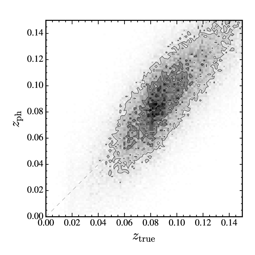
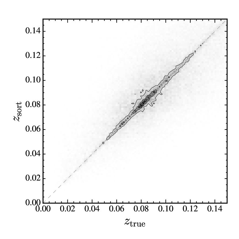
In order to test whether our sort redshift ($z_{\rm sort}$) has actually improved the redshift estimation compared to the original photometric redshifts ($z_{\rm ph}$), we directly compare them with the underlying true redshifts ($z_{\rm true}$). In Figure 3 we show two-dimensional normalized histograms for $z_{\rm ph}$ (left panel, $y$-axis) and $z_{\rm sort}$ (right panel, $y$-axis) as a function of $z_{\rm true}$ ($x$-axes). We observe that sort redshifts have a considerably reduced the scatter around the true redshifts, at least for small differences. Although barely appreciable in these plots however, we note that an underlying broader scatter remains for larger redshift differences which makes the whole distribution to have a comparable standard deviation of $\sigma\approx 0.02$.

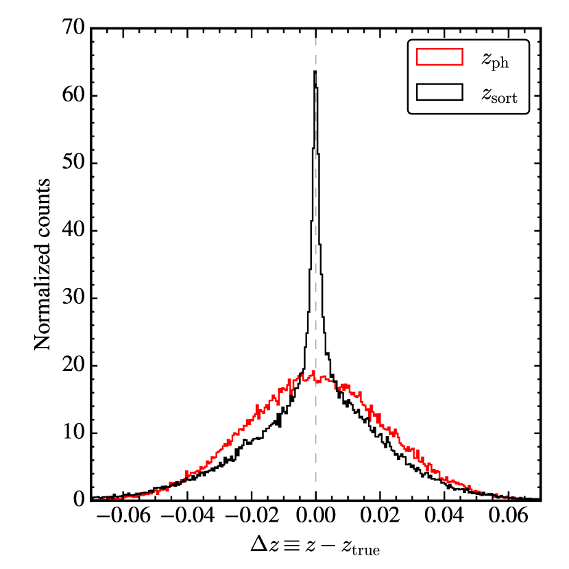
This behaviour is better illustrated in Figure 4, where we show the full redshift difference distributions for both $z_{\rm ph}$ (red histogram) and $z_{\rm sort}$ (black histogram). By construction, the original photometric sample has a Gaussian uncertainty distribution with standard deviation $\sigma_{z_{\rm ph}}\approx 0.02$. On the other hand, $z_{\rm sort}$ has a somewhat symmetric (skewness of $\approx-0.3$) uncertainty distribution with a much smaller full width at half maximum of FWHM $\approx 0.004$. This is the peak that dominates the signal in the right panel of Figure 3. If we model this narrow peak as a single Gaussian, we obtain a standard deviation of $\sigma_{z_{\rm sort}}^{\rm peak}\approx\frac{\rm FWHM}{2.4}\approx 0.0017$, which is about an order of magnitude improvement with respect to the original photometric uncertainty. At redshift differences $|\Delta z|\gtrsim 0.002$ however, the sort redshift sample has a broader underlying scatter, which makes the overall distribution have a dispersion comparable to that of the original photometric uncertainty (i.e. $\sigma_{z_{\rm sort}}\approx 0.02$).

If both distributions have comparable standard deviations, do the sort redshifts represent a real improvement over the original photometric redshifts? In order to answer this question, one must carefully consider the meaning of the standard deviation as a measure of statistical uncertainty. Indeed, it is worth reminding the reader the standard deviation alone is not enough to characterize an arbitrary PDF, even though in astronomy is widely used as the main statistical uncertainty indicator (partly because astronomers usually deal with Gaussian distributions for which such an approach is justified). The overall shape of the $\Delta z|_{\rm sort}$ distribution is not Gaussian, as it has a much more peaked distribution (and consequently more extended tails) for a similar mean ($\approx 0$) and similar standard deviation ($\approx 0.02$). Indeed, based on its kurtosis value of $\approx 5$, $\Delta z|_{\rm sort}$ resembles more a Hyperbolic Secant instead. Here we argue that a more peaked redshift uncertainty distribution around $0$ contains more information than a less peaked one, and that having a distribution like $\Delta z|_{\rm sort}$ is indeed an improvement over $\Delta z|_{\rm ph}$.

This fact can be partially appreciated by our previous comparison of the overall redshift distributions (see Figure 2, Section 4.2). We can observe that the original photometric sample not only loses information regarding the positions of the large-scale structure (i.e. peaks and valleys) but also produces biases in the expected number of galaxies as a function of redshift.

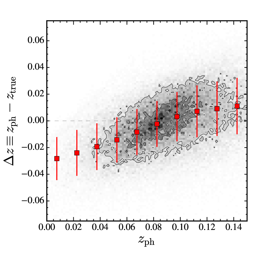
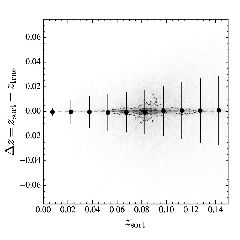
Another way to look at this issue is by quantifying the $\Delta z|_{\rm obs}\equiv z_{\rm obs}-z_{\rm true}$ as a function of $z_{\rm obs}$. In Figure 5 we show the mean of $\Delta z|_{\rm obs}$ as a function of $z_{\rm obs}=z_{\rm ph}$ (left panel) and $z_{\rm obs}=z_{\rm sort}$ (right panel). We observe that indeed the photometric sample is highly biased towards negative $\Delta z$ values at the lowest redshift bins and somewhat biased towards positive $\Delta z$ values at the highest redshift bins. In contrast, $z_{\rm sort}$ are virtually unbiased across the full redshift range which is clearly an improvement.

In the following subsections we explore how sort performs at retrieving the three-dimensional large-scale structure distribution as well as the two-point autocorrelation function.

4.3.1 Three-dimensional spatial distributions

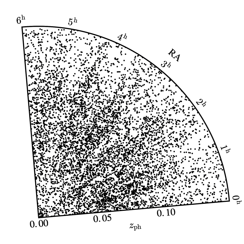
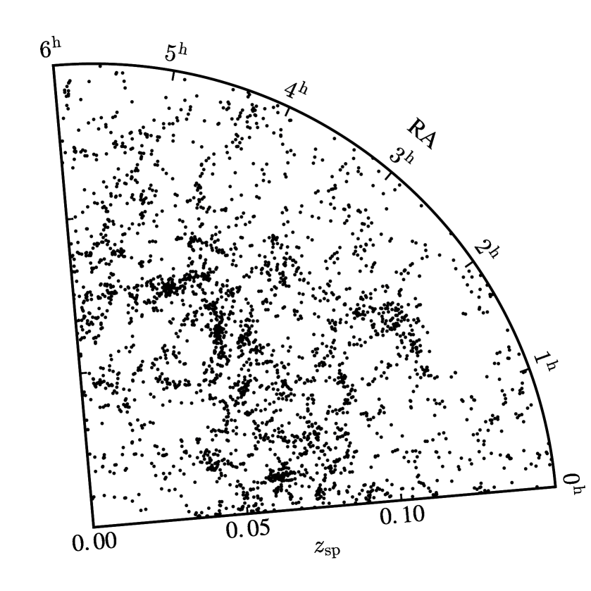
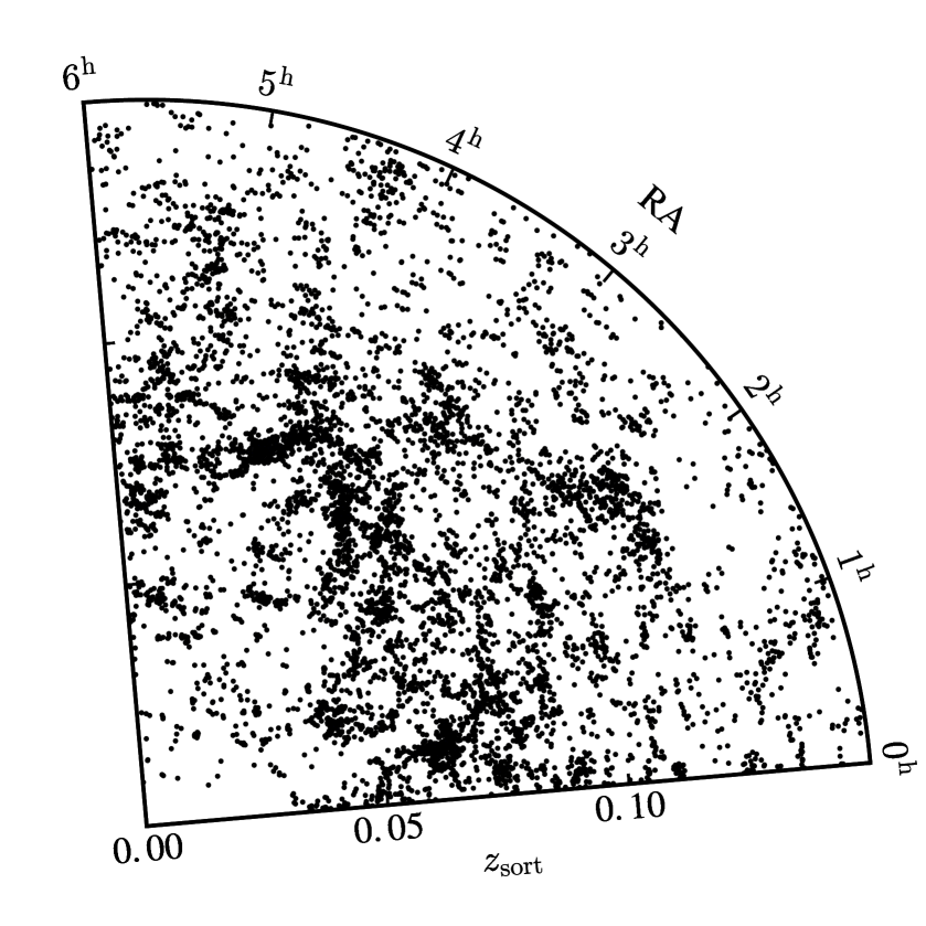
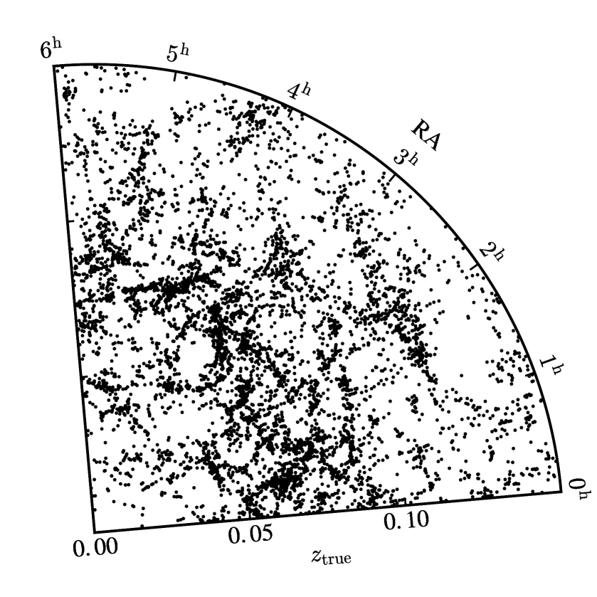
Figure 6 shows a subvolume of the mock survey, where the redshifts come from our different estimates: $z_{\rm ph}$ (top left panel), $z_{\rm sp}$ (top right panel), $z_{\rm sort}$ (bottom left panel) and $z_{\rm true}$ (bottom right panel). Unsurprisingly, the original photometric sample does not provide a good description of the cosmic web. On the other hand, our sort method is able to reproduce most of the significant large-scale-structures in the volume, including voids, dense filaments, groups and clusters (compare the two bottom panels to each other). Part of this success is due to the chosen parameters for applying the method (i.e. those relevant for the cosmic web scales; see Section 4.1) in combination with having a representative reference sample (i.e., $z_{\rm sp}$; see the top right panel of Figure 6). The recovered distribution is not perfect however and some noticeable artefacts exist. For example, the $z_{\rm sort}$ cosmic walls are thicker and the voids less empty than for $z_{\rm true}$. These should in principle be overcome by fine-tuning of the parameters for applying the method (specially $A$ and $\delta z$; see Section 4.1). Although the cosmic web seems to be reasonably well recovered as a whole, we also emphasize that there will be some individual galaxies assigned to the wrong structures along the line-of-sight, i.e. those contributing to the tails of the $\Delta z$ distribution (see Section 4.3). Still, the fact that $z_{\rm sort}$ provides a considerable fraction of galaxies assigned to the right structures along the line-of-sight (i.e. the narrow peak in $\Delta z$ distribution), makes this sort method promising for further studies aimed to quantify the three-dimensional distribution of the cosmic web and cosmological environment of galaxies using photometric redshifts.

4.3.2 Two-point correlation functions

Although the two-point correlation function (2PCF) is not enough to describe the full three-dimensional spatial distribution, it is a well defined and simple statistical measurement that contains relevant information regarding spatial clustering. As such, it has been applied to a wide variety of extragalactic questions not just related to the large-scale structure but also to galaxy evolution and cosmology.

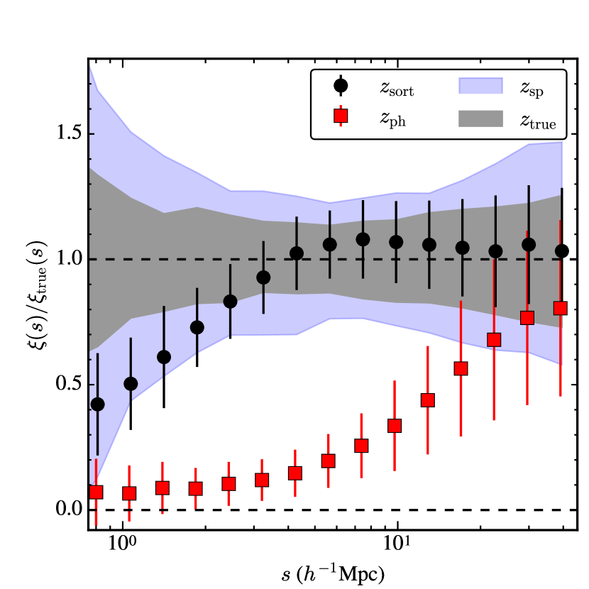
Figure 7 shows the ratio between the measured redshift space 2PCF and its true underlying value, $\xi_{\rm true}(s)$, as a function of redshift space distance $s$. The black circles correspond to using $z_{\rm sort}$ and the red squares correspond to using $z_{\rm ph}$. Uncertainties were estimated with a bootstrap technique from $100$ realizations. The grey shaded area corresponds to the intrinsic $1\sigma$ uncertainty limit due to sample variance (i.e. this is the uncertainty assuming we knew the underlying true redshift for all the galaxies in the original photometric sample). The light-blue area corresponds to the $1\sigma$ uncertainty around the unbiased measurement using the spectroscopic sample (i.e. the remaining $30\%$ of galaxies used as reference; see Section 3). This figure demonstrates that $z_{\rm sort}$ is able to recover the true 2PCF on scales $\gtrsim 4$ $h^{-1}$Mpc in a somewhat unbiased manner at a higher statistical precision than that of the reference spectroscopic sample. At smaller than $\approx 4$ $h^{-1}$Mpc scales however, $z_{\rm sort}$ is not able to recover the 2PCF power; these scales are comparable or smaller than that of the narrow peak recovered in the redshift uncertainty distribution (see Section 4.3). On the other hand, the original photometric redshift are unable to recover the 2PCF power at any scale, including those at $\gtrsim 10-40$ $h^{-1}$Mpc. We note that comparing in redshift space is conservative because the redshift uncertainties introduce distortions only along the line-of-sight. Our method preserves the observed positions of objects in the sky, ensuring that the angular correlations are not affected.

In view of these results, we argue that $z_{\rm sort}$ is not just an improvement over $z_{\rm ph}$, but it also provides more information than that contained in the reference sample used on scales $\gtrsim 4$ $h^{-1}$Mpc. We note however that sort was not particularly optimized for measuring the two-point correlation function, for which there may be other preferable methods available.

Figure 7: The ratio between the measured redshift-space two-point correlation function and its underlying true value, $\xi(s)/\xi_{\rm true}(s)$, as a function of redshift space distance $s$. The black circles correspond to using $z_{\rm sort}$ and the red squares correspond to using $z_{\rm ph}$ (slightly offset in the $x$-axis for clarity). Uncertainties were estimated from a bootstrap technique from $100$ realizations. The grey shaded area corresponds to the intrinsic $1\sigma$ uncertainty limit due to sample variance (i.e. this is the uncertainty assuming we knew the underlying true redshift for all the galaxies in the original photometric sample). The light-blue area corresponds to the $1\sigma$ uncertainty around the unbiased $z_{\rm sp}$ measurement from the spectroscopic sample (i.e. the remaining $30\%$ of galaxies used as reference). See Section 4.3.2 for further details.

5 Discussion

5.1 Where does the information come from?

Figure 8: Redshift difference $\Delta z\equiv z-z_{\rm true}$ for our different redshift measurements: $z_{\rm sort}$ (black), $z_{\rm ph}$ (red), $z_{\rm ctrl}$ (orange), $z_{\rm sort+}$ (green). The left panel shows a log-linear scale, while the right panel presents a zoom-in of the peak in a linear scale. See Section 5.1 for details.

.

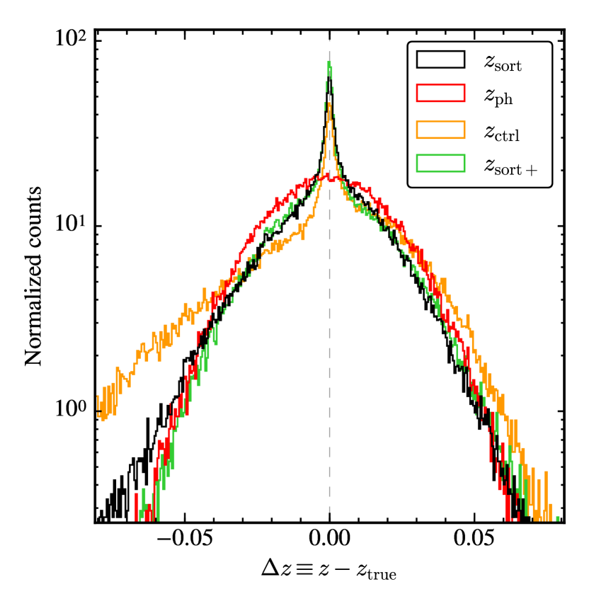
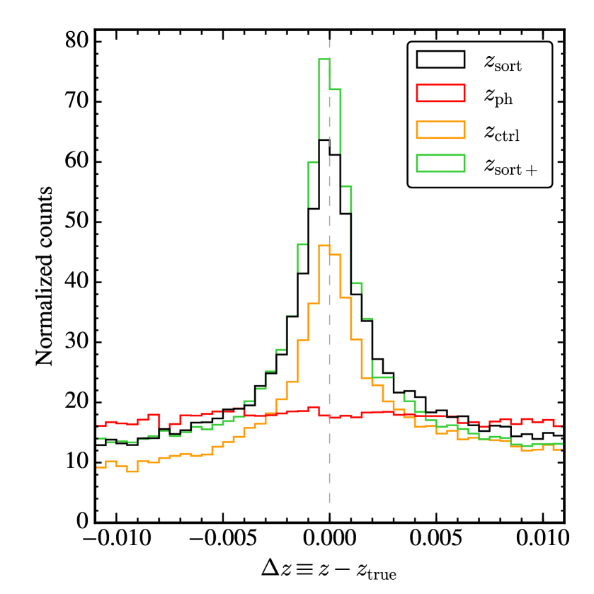
A relevant question to ask in the context of our method is where the information comes from. Certainly, the use of a reference sample must contribute a significant amount, but how much of an improvement does the stochastic ordering matching scheme signify (see Section 2.2)? In order to answer this question we have run a control method using exactly the same algorithm presented in Section 4.1 but replacing the fifth step simply with a random one-to-one assignment scheme instead (i.e. no rank ordering was applied). We call this control redshift assignment, $z_{\rm ctrl}$. In the following we will use the $\Delta z\equiv z-z_{\rm true}$ normalized histograms as proxies of the underlying redshift PDFs for our different methods. In principle, a narrower and more peaked PDF contains more information than a broader and less peaked one.

Figure 8 shows versions of Figure 4 including $z_{\rm ctrl}$ (orange histograms) and $z_{\rm ctrl+}$ (green histograms; described below); $z_{\rm sort}$ (black histograms) and $z_{\rm ph}$ (red histograms) are the same as in Figure 8. The left panel shows $\Delta z$ histograms in logarithmic scale, allowing us to emphasize the behaviour of the tails of the distributions. The right panel shows $\Delta z$ histograms in linear scale, with emphasis on the narrow peak. Comparing the orange ($z_{\rm ctrl}$) to the black ($z_{\rm sort}$) histograms we see that the stochastic ordering provides extra information: the tails are more symmetrical and more suppressed, and the peak of around $\Delta z=0$ is higher.

From Figure 8 we can also see that $z_{\rm sort}$ is not necessarily the most optimal redshift estimation because at the $|\Delta z|$ tails, there is a (small) contribution of $z_{\rm sort}$ redshifts whose differences with respect to their true values are larger than what would be allowed by the original photometric PDF, i.e. catastrophic redshift assignments. We remind the reader that in obtaining $z_{\rm sort}$ we have so far not used the information provided by the individual $z_{\rm ph}$ uncertainties, but only their most likely redshift values. (This was a deliberate choice in order emphasize the intrinsic power of the stochastic order.) In order to take into account the full individual $z_{\rm ph}$ PDFs, one can simply convolve these with the distributions obtained at the end of the algorithm presented in Section 4.1 to increase the quality of the sort. We call the redshifts from this optimal sort method $z_{\rm sort+}$, and its redshift uncertainty distribution is shown as the green histograms in Figure 8. We see that indeed, $z_{\rm sort+}$ ensures a tail no larger than that of the original $z_{\rm ph}$, and has a greater peak than that of $z_{\rm sort}$.

We conclude that although a significant amount of information comes from the use of the reference sample, the stochastic order matching scheme does indeed add valuable extra information. In particular, sort significantly improves the quality of the recovered redshift PDF, as it reduces the global asymmetry, suppresses the large tails, and makes a more pronounced peak around $\Delta z=0$. Moreover, an extra enhancement can be easily achieved by using the information provided by the full photometric PDFs rather than only the most likely value alone.

Figure 9: Left panel: redshift difference $\Delta z\equiv z_{\rm sort}-z_{\rm true}$ using different percentages of galaxies as reference (spectroscopic): $f_{\rm sp}=30\%$ (our fiducial value; black histogram), $f_{\rm sp}=10\%$ (blue histogram) and $f_{\rm sp}=5\%$ (orange histogram). As reference, the original $\Delta z=z_{\rm ph}-z_{\rm true}$ distribution is shown as a shaded grey. Right panel: redshift difference $\Delta z\equiv z_{\rm sort}-z_{\rm true}$ using different values for the original redshift uncertainties: $\sigma_{z}^{\rm ph}=0.02$ (our fiducial value; black histogram), $\sigma_{z}^{\rm ph}=0.05$ (green histogram) and $\sigma_{z}^{\rm ph}=0.1$ (red histogram). As reference, the original $\Delta z=z_{\rm ph}-z_{\rm true}$ distributions are shown as the shaded grey, light-green and light-red histograms, respectively. See Section 5.2 for further details.

5.2 Versatility and efficiency

Perhaps one of the most attractive qualities of sort is its simplicity, which in turns makes it very versatile. Indeed, in its general form the projected area $A$ can have any arbitrary shape and size. Thus, the method can be applied to wide and narrow extragalactic surveys alike (provided that suitable reference samples exist). We also emphasize that sort is intrinsically a non-parametric method, as we are not assuming any functional form on the shape of the galaxy distributions along individual lines-of-sight, nor on the luminosity function of galaxies. Similarly, we are not applying convolutions nor de-convolutions in order to infer the intrinsic underlying true redshifts, which is advantageous in the sense that information is not being deliberately lost.

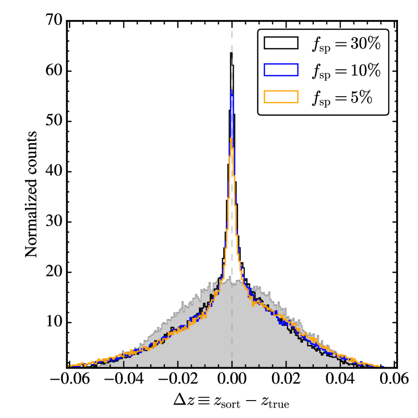
Besides its versatility, sort is also intrinsically efficient. The most expensive requirement of the method is the use of a suitable spectroscopic reference sample. However, considering that a significant fraction of luminous galaxies reside in a small fraction of the volume (i.e. luminous galaxies are biased tracers of the underlying clustered matter distribution), then small reference samples can still give a sensible mapping of the structures along a given line-of-sight. If this is the case, then our proposed sort should still perform relatively well even using small reference samples. In order to illustrate this point, in the left panel of Figure 9 we show normalized $\Delta z\equiv z_{\rm sort}-z_{\rm true}$ for three sort realizations (using the algorithm presented in Section 4.1), each one applied to mock galaxy surveys as described in Section 3 having three different percentages of reference spectroscopic galaxies: $f_{\rm sp}=30\%$ (our fiducial value; black histogram), $f_{\rm sp}=10\%$ (blue histogram) and $f_{\rm sp}=5\%$ (orange histogram). As expected, the lower the fractions of galaxies used as reference, the poorer the quality of the recovered $z_{\rm sort}$. Still, we see that even when using a reference sample as small as $\sim 5\%$, sort is able to improve over the original photometric redshifts.

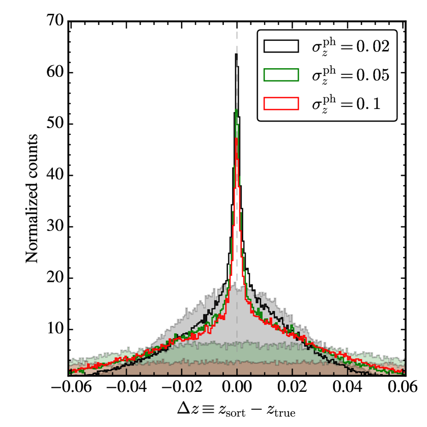
Moreover, as pointed out in Section 2.2, if the individual photometric redshift PDFs satisfy Equation 9 (i.e. stochastic order), then the method should perform relatively well independently of the actual value of the photometric redshift uncertainty. This is illustrated in the right panel of Figure 9, where we show normalized $\Delta z\equiv z_{\rm sort}-z_{\rm true}$ distributions for three levels of photometric redshift uncertainty: $\sigma_{z}^{\rm ph}=0.02$ (black histogram; our fiducial value), $\sigma_{z}^{\rm ph}=0.05$ (green histogram) and $\sigma_{z}^{\rm ph}=0.1$ (red histogram). We observe that the narrow peak around $\Delta z=0$ is also well recovered using $\sigma_{z}^{\rm ph}=0.05$ or $\sigma_{z}^{\rm ph}=0.1$. Although the quality of the recovered $z_{\rm sort}$ is higher for lower $\sigma_{z}^{\rm ph}$, we emphasize that the relative improvement over the original $z_{\rm ph}$ is actually higher for larger $\sigma_{z}^{\rm ph}$. Indeed, in the later cases even the standard deviation of $\Delta z$ is substantially reduced, from the original values of $\sigma_{z}\approx 0.05$ and $\sigma_{z}\approx 0.1$ both to $\sigma_{z}\approx 0.03$.

We also consider sort to be an efficient method in terms of computational time. Indeed, the fact that sort provides improved cosmological redshifts for samples rather than individual objects, can significantly reduce the cost of the method in CPU time. Additionally, the most time consuming part of the algorithm, i.e. the adaptive Monte Carlo realizations, can be easily parallelized as these are all independent of each other.

5.3 Applications

We consider that the main application for a method like sort would be to recover the distinctive features of the cosmic web, i.e. estimating the locations of voids, filaments and walls. These can then be used for studies of galaxy evolution as a function of large-scale environment, by enabling individual galaxies to be located in their corresponding cosmic web structures along the line-of-sight. Similarly, the sort redshifts can be used to estimate environmental density on scales $\sim 4$ $h^{-1}$Mpc, which correlates (directly or indirectly) with several properties of dark matter halos (e.g. Lee et al., 2017) or galaxies (e.g. Yan et al., 2013; Eardley et al., 2015). This application can also be extended to studies of the intergalactic medium (IGM) in different cosmic environment traced by galaxies (e.g. Penton et al., 2002; Stocke et al., 2007; Tejos et al., 2012, 2016); given that the IGM is usually detected through absorption lines in the spectra of background QSOs, a method that could correctly identify cosmic web structures in pencil-beam-like galaxy surveys becomes particularly useful and efficient.

Another potential application may be on the characterization the intrinsic properties of these large-scale structures, in particular their shapes. Indeed, there is relevant cosmological information imprinted in the size distribution of galaxy voids, their relative underdensities, their density profiles, among others (e.g. Sutter et al., 2014a, b; Cai et al., 2015; Hamaus et al., 2015; Massara et al., 2015; Yang et al., 2015; Hamaus et al., 2016, 2017; Kovács et al., 2017). It is still to be seen whether sort redshifts can be used to improve results on these cosmological tests.

5.4 Limitations

As any method, sort does not lack limitations. The most obvious one is the need of a reference sample to map out the real structures along the line-of-sight. As shown in Section 5.1, most of the information comes from the reference sample. Then, if for some reason a structure is not covered by the reference, sort will not be able to recover such structure. Similarly, there is also the intrinsic limit imposed by the actual velocity dispersion of galaxies within the large-scale-structure of $\Delta v\approx 200$ km s^-1, corresponding to redshift differences of $\delta z\approx 0.001$ (or $\sim 3$ $h^{-1}$Mpc), which prevents sort from reaching higher precisions.

An additional limitation comes from the actual selection functions for both the photometric (uncertain) and the spectroscopic (reference) samples, $S_{\rm ph}$ and $S_{\rm sp}$ (see Section 2.1), in the sense that relevant information is only obtained for the redshifts range where both overlap. In the extreme case where $S_{\rm ph}$ and $S_{\rm sp}$ are disjoint, our method cannot be applied. Similarly, if the objects used as reference trace the cosmic web differently than those in the uncertain sample (as it may be the case for quasars versus dwarfs galaxies), then our method will introduce a systematic error by wrongly assigning the uncertain sample to match the cosmic web of the reference. Of course, one can avoid this potential bias by making sure that the reference sample is statistically relevant to that of the uncertain one before applying sort.

Another intrinsic limitation of the method is that the recovered mapping of structures is only robust for the full ensemble, but not necessarily for individual objects. This comes from the fact that we cannot distinguish which individual galaxies contribute to the peak of the $\Delta z$ distribution, and which ones contribute to the tails. This means that despite having a sensible reconstruction of the three-dimensional distributions (see Section 4.3.1) and/or the two-point correlation function on scales $\gtrsim 4$ $h^{-1}$Mpc, there will be galaxies assigned to the wrong structures along the line-of-sight. Although $z_{\rm sort}$ could be in principle used to define large-scale environments (voids, filaments, clusters), still a more precise redshift estimation will be needed to place individual galaxies into these environments.

We also note that the efficiency of sort is limited by the choice of the projected area $A$ to define sub-volumes. Let us consider two extreme cases as examples. When $A\to 0$ the method will be applied to individual galaxies rather than the ensemble, reducing its efficiency (1) because we loose the information provided by the angular correlations, and (2) because we need a comparatively larger fraction of galaxies in the reference sample (more expensive). On the other hand, when $A\to 4\pi$ the method will be applied to the whole sky, reducing its efficiency because the information provided by the angular correlations as a function of redshift will be washed out (although it may still work for very local cosmological structures). For simplicity, in this paper we have used a circular $A$ of radius $1$ degree chosen because it corresponds to $\approx 5-10$ $h^{-1}$Mpc at the redshifts where most of our galaxies reside (see Section 4.1). In principle however, there should exist an optimal $A$ that maximizes the amount of information recovered by sort. This optimal $A$ has to be small enough to resolve the angular correlations introduced by galaxy clustering as a function of redshift, and large enough to include a minimum number of reference redshifts ensuring a sensible mapping of the structures. Thus, this optimal $A$ has to be a function of redshift $A(z)$ and also a function of the survey design. For instance, given the behaviour of transverse distance as a function of redshift, we expect that for $z>1$, an optimal $A$ containing transverse scales up to $\sim 5-10$ $h^{-1}$Mpc could be as small as a tenth of a degree (i.e. few arcmins), making sort particularly promising for future generations of deep pencil-beam-like surveys. Obtaining a general optimization of $A$ is beyond the scope of this paper. Surveys such as COSMOS and CANDELS would be ideal to put constraints on the optimal $A(z)$ function and test the limitations of sort.

5.5 Comparison to previous work and complementarity

In this section we provide a comparison with two recent relevant published methods, namely the PhotoWeb (Aragon-Calvo et al., 2015) and the clustering-based redshift estimation (Ménard et al., 2013).

Comparison to PhotoWeb Our method has many similarities with the PhotoWeb proposed by Aragon-Calvo et al. (2015). Both methods rely on the presence of an statistically relevant reference sample tracing an underlying ‘cosmic web’ of structures along the line-of-sight, and both methods use this reference sample in order to improve photometric redshifts. However, an important difference between SORT and PhotoWeb is that the latter acts on individual galaxies rather than an ensemble. This is both advantageous and disadvantageous. The advantage is that PhotoWeb can reconstruct the underlying density field in a given line-of-sight at a much better resolution than that of SORT; the disadvantage is that PhotoWeb does not necessarily preserve $dN/dz(z)$ as it tends to over-represent galaxy over-densities and under-represent the galaxy under-densities. In other words, their voids are too empty and their walls are too populated. This is because the improved PhotoWeb redshift estimation comes from multiplying different PDFs (i.e. density, geometrical and photometric, see their equation 1) of individual galaxies independently of the recovered redshifts of the others. On the other hand, sort starts from the condition that the $dN/dz$ of the reference sample has to be preserved, and only uses the photometric individual PDFs to establish their final rank order in redshift.

Regarding the $\Delta z\equiv z-z_{\rm true}$ recovered distributions, both techniques give similar shapes (see their figure 9). Although Aragon-Calvo et al. (2015) have modelled it as the combination of two Gaussians, here we have argued that based on its kurtosis value, a Hyperbolic Secant may be more appropriate description (see Section 4.3). Moreover, they have used the width of the narrow peak to claim a sub-megaparsec precision (i.e. redshift uncertainty as low as $\approx 0.0007$). However, because there is no way to determine which individual galaxies contribute to the narrow peak as opposed to the broader $\Delta z$ distribution, such a low uncertainty estimation is way too optimistic.

Comparison to the clustering-based redshift estimation Another relevant recent work to compare with is that of Ménard et al. (2013). In contrast to sort or PhotoWeb, the clustering-based method relies on a reference sample (e.g. spectroscopic) but it only requires the existence of a non-zero two-point correlation function, which is a weaker constraint that requiring a well defined ‘cosmic web’. The clustering-based method is fully independent from the original photometric redshift estimation, as it only uses the information given by the spatial clustering of the sources. In this manner, the resulting clustering-based redshift PDF can be multiplied with the independent photometric redshift PDF to obtain an improved cosmological redshift for individual sources. The essence of their method is to divide the survey volume into multiple narrow redshift slices, and for a given slice to identify the subsample of galaxies that maximise the projected angular correlation to that of the respective reference sample while making sure the $dN/dz$ is also preserved. This is in contrast to our sort method, where we divide the survey volume into multiple pencil-beam like surveys and impose the photometric samples to match the $dN/dz$ of the respective reference sample in each of those sub-volumes, while also preserving their rank order in redshift.

Because of its intrinsic simplicity and versatility (see Section 5.2), we envision that a method like sort could be integrated into these more complex and sophisticated algorithms aimed at improving cosmological redshifts.

5.6 Future prospects

The obvious next step is to apply sort to real data (e.g. SDSS), for which an accounting of the more complex selection function and individual photometric redshift PDFs must be taken into account. In such a case, the method should be calibrated against a realistic mock survey for optimization.

Of particular interest for the upcoming large photometric surveys (e.g. LSST), is to explore the efficiency of the method when using much fainter galaxies, and whether or not one can effectively use brighter (cheaper) galaxies as reference to recover the structures along a given line-of-sight. Similarly, one can also produce forecasts on how well the large-scale structures (voids, walls, filaments, clusters) can be recovered using sort, and the impact of such reconstruction on weak-lensing mapping, the recovery of the baryonic acoustic oscillations (BAO), etc.

There is also some room for improvement of the method in terms of using other galaxy properties beyond position alone, such as star-formation activity, colour, shapes, etc. Moreover, our current implementation does not explicitly take into account the clustering information within the projected area $A$. Indeed, by assuming a functional form of the spatial clustering of galaxies one could assign join probabilities for galaxies to be at a similar redshifts if they appear highly clustered within $A$; such information can help to better constrain the original individual PDFs, hence improving the overall performance of sort. Although we expect our method to apply mostly to field galaxies, for wider applications it will be necessary to compensate for large galaxy redshift distortions introduced by galaxy clusters (i.e. the so-called fingers-of-god), which could be done using standard techniques (e.g. Tegmark et al., 2004; Aragon-Calvo et al., 2015).

In a more general context, we believe that the main strengths of sort are its simplicity and its versatility; hence, it would make more sense to use it in combination with some other more sophisticated method aimed at improving cosmological redshifts (e.g. Ménard et al., 2013; Aragon-Calvo et al., 2015).

6 Summary and conclusions

In this paper we have presented a simple, efficient and robust method to improve cosmological redshifts with uncertainties larger than the ‘cosmic web’ scales ($\gtrsim 3$ $h^{-1}$Mpc). The method is based on the presence of a reference sample for which a precise redshift number distribution ($dN/dz$) can be obtained for different pencil-beam-like sub-volumes within the original survey. For each sub-volume we then impose:

• (i) that the redshift number distribution of the uncertain redshift measurement matches the reference $dN/dz$ corrected by their selection functions; and

• (ii) the rank order in redshift of the original ensemble of uncertain redshift measurements is preserved.

The latter step is motivated by the fact that random variables drawn from Gaussian probability density functions (PDFs) of different means and arbitrarily large standard deviations satisfy stochastic ordering. We then repeat this simple algorithm for multiple arbitrary pencil-beam-like overlapping sub-volumes; in this manner, each uncertain measurement has multiple (non-independent) “recovered” redshifts which can be used to estimate a new redshift PDF. Assuming that redshift measurements can be treated as random variables, we thus refer to this method as the Stochastic Order Redshift Technique (sort).

We have used a state-of-the art $N$-body simulation to test the performance of sort under simple assumptions and found that it can improve the quality of cosmological redshifts in an efficient manner. Particularly, sort redshifts ($z_{\rm sort}$) are able to recover the distinctive features of the so-called ‘cosmic web’ and can provide unbiased measurement of the two-point correlation function on scales $\gtrsim 4$ $h^{-1}$Mpc. Based on these results, we have argued that sort provides more information than that of the reference sample alone.

Given its simplicity, we envision that a method like sort can be incorporated into more sophisticated algorithms aimed to exploit the full potential of large extragalactic photometric surveys. Indeed, most of the state-of-the-art photometric (and clustering based) redshift algorithms reach individual statistical precisions of $\sigma_{z}\approx 0.02-0.05$ (Gaussian). In this paper we have shown that such precision can be further improved applying an extremely simple, efficient and robust method that relies on stochastic order.

References

- Aragon-Calvo et al. (2016) Aragon-Calvo M. A., Neyrinck M. C., Silk J., 2016, ArXiv:1607.07881
- Aragon-Calvo et al. (2015) Aragon-Calvo M. A., Weygaert R. v. d., Jones B. J. T., Mobasher B., 2015, MNRAS, 454, 463
- Arnalte-Mur et al. (2014) Arnalte-Mur P., Martínez V. J., Norberg P., Fernández-Soto A., Ascaso B., Merson A. I., Aguerri J. A. L., Castander F. J. et al, 2014, MNRAS, 441, 1783
- Astropy Collaboration et al. (2013) Astropy Collaboration, Robitaille T. P., Tollerud E. J., Greenfield P., Droettboom M., Bray E., Aldcroft T., Davis M. et al, 2013, A&A, 558, A33
- Beck et al. (2016) Beck R., Dobos L., Budavári T., Szalay A. S., Csabai I., 2016, MNRAS, 460, 1371
- Behroozi et al. (2013) Behroozi P. S., Wechsler R. H., Wu H.-Y., 2013, ApJ, 762, 109
- Bos et al. (2012) Bos E. G. P., van de Weygaert R., Dolag K., Pettorino V., 2012, MNRAS, 426, 440
- Cai et al. (2015) Cai Y.-C., Padilla N., Li B., 2015, MNRAS, 451, 1036
- Cen & Ostriker (1999) Cen R., Ostriker J. P., 1999, ApJ, 514, 1
- Cole et al. (2005) Cole S., Percival W. J., Peacock J. A., Norberg P., Baugh C. M., Frenk C. S., Baldry I., Bland-Hawthorn J. et al, 2005, MNRAS, 362, 505
- Cunha et al. (2009) Cunha C. E., Lima M., Oyaizu H., Frieman J., Lin H., 2009, MNRAS, 396, 2379
- Dark Energy Survey Collaboration et al. (2016) Dark Energy Survey Collaboration, Abbott T., Abdalla F. B., Aleksić J., Allam S., Amara A., Bacon D., Balbinot E. et al, 2016, MNRAS, 460, 1270
- Davé et al. (2001) Davé R., Cen R., Ostriker J. P., Bryan G. L., Hernquist L., Katz N., Weinberg D. H., Norman M. L. et al, 2001, ApJ, 552, 473
- Eardley et al. (2015) Eardley E., Peacock J. A., McNaught-Roberts T., Heymans C., Norberg P., Alpaslan M., Baldry I., Bland-Hawthorn J. et al, 2015, MNRAS, 448, 3665
- Flaugher (2012) Flaugher B., 2012, in APS April Meeting Abstracts
- Gillet et al. (2015) Gillet N., Ocvirk P., Aubert D., Knebe A., Libeskind N., Yepes G., Gottlöber S., Hoffman Y., 2015, ApJ, 800, 34
- Grogin et al. (2011) Grogin N. A., Kocevski D. D., Faber S. M., Ferguson H. C., Koekemoer A. M., Riess A. G., Acquaviva V., Alexander D. M. et al, 2011, ApJS, 197, 35
- Hamaus et al. (2017) Hamaus N., Cousinou M.-C., Pisani A., Aubert M., Escoffier S., Weller J., 2017, JCAP, 7, 014
- Hamaus et al. (2016) Hamaus N., Pisani A., Sutter P. M., Lavaux G., Escoffier S., Wandelt B. D., Weller J., 2016, Physical Review Letters, 117, 091302
- Hamaus et al. (2015) Hamaus N., Sutter P. M., Lavaux G., Wandelt B. D., 2015, JCAP, 11, 036
- Klypin et al. (2016) Klypin A., Yepes G., Gottlöber S., Prada F., Heß S., 2016, MNRAS, 457, 4340
- Koekemoer et al. (2007) Koekemoer A. M., Aussel H., Calzetti D., Capak P., Giavalisco M., Kneib J.-P., Leauthaud A., Le Fèvre O. et al, 2007, ApJS, 172, 196
- Koekemoer et al. (2011) Koekemoer A. M., Faber S. M., Ferguson H. C., Grogin N. A., Kocevski D. D., Koo D. C., Lai K., Lotz J. M. et al, 2011, ApJS, 197, 36
- Kovács et al. (2017) Kovács A., Sánchez C., García-Bellido J., Nadathur S., Crittenden R., Gruen D., Huterer D., Bacon D. et al, 2017, MNRAS, 465, 4166
- Landy et al. (1996) Landy S. D., Szalay A. S., Koo D. C., 1996, ApJ, 460, 94
- Lee et al. (2016) Lee B. C. G., Budavári T., Basu A., Rahman M., 2016, AJ, 152, 155
- Lee et al. (2017) Lee C. T., Primack J. R., Behroozi P., Rodríguez-Puebla A., Hellinger D., Dekel A., 2017, MNRAS, 466, 3834
- Li (2011) Li B., 2011, MNRAS, 411, 2615
- Lima et al. (2008) Lima M., Cunha C. E., Oyaizu H., Frieman J., Lin H., Sheldon E. S., 2008, MNRAS, 390, 118
- LSST Science Collaboration et al. (2009) LSST Science Collaboration, Abell P. A., Allison J., Anderson S. F., Andrew J. R., Angel J. R. P., Armus L., Arnett D. et al, 2009, ArXiv:0912.0201
- Lu et al. (2015) Lu Y., Mo H. J., Lu Z., 2015, ArXiv:1504.02109
- Massara et al. (2015) Massara E., Villaescusa-Navarro F., Viel M., Sutter P. M., 2015, JCAP, 11, 018
- McQuinn & White (2013) McQuinn M., White M., 2013, MNRAS, 433, 2857
- Ménard et al. (2013) Ménard B., Scranton R., Schmidt S., Morrison C., Jeong D., Budavari T., Rahman M., 2013, ArXiv:1303.4722
- Mo et al. (2005) Mo H. J., Yang X., van den Bosch F. C., Katz N., 2005, MNRAS, 363, 1155
- Padmanabhan et al. (2005) Padmanabhan N., Budavári T., Schlegel D. J., Bridges T., Brinkmann J., Cannon R., Connolly A. J., Croom S. M. et al, 2005, MNRAS, 359, 237
- Peng et al. (2015) Peng Y., Maiolino R., Cochrane R., 2015, Nature, 521, 192
- Peng et al. (2010) Peng Y.-j., Lilly S. J., Kovač K., Bolzonella M., Pozzetti L., Renzini A., Zamorani G., Ilbert O. et al, 2010, ApJ, 721, 193
- Penton et al. (2002) Penton S. V., Stocke J. T., Shull J. M., 2002, ApJ, 565, 720
- Phillipps & Shanks (1987) Phillipps S., Shanks T., 1987, MNRAS, 227, 115
- Planck Collaboration et al. (2016) Planck Collaboration, Ade P. A. R., Aghanim N., Arnaud M., Ashdown M., Aumont J., Baccigalupi C., Banday A. J. et al, 2016, A&A, 594, A13
- Plionis & Basilakos (2002) Plionis M., Basilakos S., 2002, MNRAS, 330, 399
- Rahman et al. (2016a) Rahman M., Ménard B., Scranton R., 2016a, MNRAS, 457, 3912
- Rahman et al. (2016b) Rahman M., Mendez A. J., Ménard B., Scranton R., Schmidt S. J., Morrison C. B., Budavári T., 2016b, MNRAS, 460, 163
- Rodríguez-Puebla et al. (2016) Rodríguez-Puebla A., Behroozi P., Primack J., Klypin A., Lee C., Hellinger D., 2016, MNRAS, 462, 893
- Scoville et al. (2007) Scoville N., Aussel H., Brusa M., Capak P., Carollo C. M., Elvis M., Giavalisco M., Guzzo L. et al, 2007, ApJS, 172, 1
- Shaked & Shanthikumar (2007) Shaked M., Shanthikumar G., 2007, Stochastic Orders
- Sheth (2007) Sheth R. K., 2007, MNRAS, 378, 709
- Shull et al. (2012) Shull J. M., Smith B. D., Danforth C. W., 2012, ApJ, 759, 23
- Stocke et al. (2007) Stocke J. T., Danforth C. W., Shull J. M., Penton S. V., Giroux M. L., 2007, ApJ, 671, 146
- Sutter et al. (2014a) Sutter P. M., Lavaux G., Wandelt B. D., Weinberg D. H., Warren M. S., 2014a, MNRAS, 438, 3177
- Sutter et al. (2014b) Sutter P. M., Pisani A., Wandelt B. D., Weinberg D. H., 2014b, MNRAS, 443, 2983
- Tegmark et al. (2004) Tegmark M., Blanton M. R., Strauss M. A., Hoyle F., Schlegel D., Scoccimarro R., Vogeley M. S., Weinberg D. H. et al, 2004, ApJ, 606, 702
- Tejos et al. (2012) Tejos N., Morris S. L., Crighton N. H. M., Theuns T., Altay G., Finn C. W., 2012, MNRAS, 425, 245
- Tejos et al. (2016) Tejos N., Prochaska J. X., Crighton N. H. M., Morris S. L., Werk J. K., Theuns T., Padilla N., Bielby R. M. et al, 2016, MNRAS, 455, 2662
- Vale & Ostriker (2004) Vale A., Ostriker J. P., 2004, MNRAS, 353, 189
- Yan et al. (2013) Yan H., Fan Z., White S. D. M., 2013, MNRAS, 430, 3432
- Yang et al. (2015) Yang L. F., Neyrinck M. C., Aragón-Calvo M. A., Falck B., Silk J., 2015, MNRAS, 451, 3606
- Yang et al. (2009) Yang X., Mo H. J., van den Bosch F. C., 2009, ApJ, 695, 900