Model-independent determination of the strong phase difference between $D^{0}$ and $\kern 1.99997pt\overline{\kern-1.99997ptD}{}^{0}\!\rightarrow\pi^{+}\pi^{-}\pi^{+}\pi^{-}$ amplitudes.

Abstract

For the first time, the strong phase difference between $D^{0}$ and $\kern 1.99997pt\overline{\kern-1.99997ptD}{}^{0}\!\rightarrow\pi^{+}\pi^{-}\pi^{+}\pi^{-}$ amplitudes is determined in bins of the decay phase space. The measurement uses 818$\mbox{\,pb}^{-1}$ of $e^{+}e^{-}$ collision data that is taken at the $\psi(3770)$ resonance and collected by the CLEO-c experiment. The measurement is important for the determination of the $C\!P$-violating phase $\gamma$ in $B^{\pm}\!\rightarrow DK^{\pm}$ (and similar) decays , where the $D$ meson (which represents a superposition of $D^{0}$ and $\kern 1.99997pt\overline{\kern-1.99997ptD}{}^{0}$) subsequently decays to $\pi^{+}\pi^{-}\pi^{+}\pi^{-}$. To obtain optimal sensitivity to $\gamma$, the phase space of the $D\!\rightarrow\pi^{+}\pi^{-}\pi^{+}\pi^{-}$ decay is divided into bins based on a recent amplitude model of the decay. Although an amplitude model is used to define the bins, the measurements obtained are model-independent. The $C\!P$-even fraction of the $D\!\rightarrow\pi^{+}\pi^{-}\pi^{+}\pi^{-}$ decay is determined to be $F_{+}^{4\pi}=0.769\pm 0.021\pm 0.010$, where the uncertainties are statistical and systematic, respectively. Using simulated $B^{\pm}\!\rightarrow DK^{\pm},D\!\rightarrow\pi^{+}\pi^{-}\pi^{+}\pi^{-}$ decays, it is estimated that by the end of the current LHC run, the LHCb experiment could determine $\gamma$ from this decay mode with an uncertainty of $(\pm 10\pm 7)^{\circ}$, where the first uncertainty is statistical based on estimated LHCb event yields, and the second is due to the uncertainties on the parameters determined in this paper.

1 Introduction

A primary goal in modern flavour physics is to constrain the unitarity triangle (UT); an abstract representation of the famous Cabibbo-Kobayashi-Maskawa matrix that describes transitions between different quark flavours CKMCabibbo ; CKM . Key to determining the UT is are better experimental constraints on the angle $\gamma$ (or $\phi_{3}$), which is related to the phase difference between $b\rightarrow u\ W^{-}$ and $b\rightarrow c\ W^{-}$ quark transitions. Currently, $\gamma$ is the least-well constrained angle of the UT, and can be determined, for example, using $B^{-}\!\rightarrow DK^{-}$ decays, where $D$ represents a superposition of $D^{0}$ and $\kern 1.99997pt\overline{\kern-1.99997ptD}{}^{0}$ states GLW1 ; GLW2 ; ADS ; DalitzGamma1 ; DalitzGamma2 ; Rademacker:2006zx . The amplitudes $B^{-}\!\rightarrow\kern 1.99997pt\overline{\kern-1.99997ptD}{}^{0}K^{-}$ and $B^{-}\!\rightarrow D^{0}K^{-}$ are overwhelmingly dominated by the tree-level transitions $b\rightarrow u\,\overline{}cs$ and $b\rightarrow c\,\overline{}us$, respectively, and therefore offer an extremely clean method to measure $\gamma$. In order to obtain the necessary interference between $B^{-}\!\rightarrow D^{0}K^{-}$ and $B^{-}\!\rightarrow\kern 1.99997pt\overline{\kern-1.99997ptD}{}^{0}K^{-}$ amplitudes, a final state $f$ must be chosen that is accessible from both $D^{0}$ and $\kern 1.99997pt\overline{\kern-1.99997ptD}{}^{0}$, such as $\pi^{+}\pi^{-}\pi^{+}\pi^{-}$ ($4\pi^{\pm}$).

To determine $\gamma$ in $B^{-}\!\rightarrow DK^{-}$ decays, one must know the relative magnitude and phase of $D^{0}\!\rightarrow f$ and $\kern 1.99997pt\overline{\kern-1.99997ptD}{}^{0}\!\rightarrow f$ amplitudes, collectively known as the $D\!\rightarrow f$ hadronic parameters. The relative magnitudes can be determined by measuring $D^{*+}\!\rightarrow D^{0}\pi^{+}$ decays that are subsequently followed by a $D^{0}\!\rightarrow f$ decay; this is possible at a large variety of collider experiments, such as LHCb and the $B$-factories. Measuring the relative phase, however, is more challenging. One method is to infer the relative phase through use of an amplitude model; in principle this is the best way to exploit the available statistics, but theoretical uncertainties in determining the model can lead to large systematic uncertainties on $\gamma$. The relative phase can also be determined model-independently by using samples of $D\!\rightarrow f$ decays, where the $D$ meson is in a known superposition of $D^{0}$ and $\kern 1.99997pt\overline{\kern-1.99997ptD}{}^{0}$ states. Previously, such data samples have been obtained from two sources: correlated $D\kern 1.99997pt\overline{\kern-1.99997ptD}{}$ pairs from the decay of a $\psi(3770)$ meson gammaADS ; ModelIndepGammaTheory ; coherenceCLEO ; Libby:2010nu ; Briere:2009aa ; CLEO:DeltaKpi ; Insler:2012pm ; Libby:2014rea (the first charmonia resonance above the charm threshold); and the decay $D^{*+}\!\rightarrow D\pi^{+}$, where the superposition of $D^{0}$ and $\kern 1.99997pt\overline{\kern-1.99997ptD}{}^{0}$ states depends on the $D$ meson decay-time  selfcite ; selfcite2 ; K3piLHCb . In this paper we determine the relative magnitude and phase of $D^{0}\!\rightarrow 4\pi^{\pm}$ and $\kern 1.99997pt\overline{\kern-1.99997ptD}{}^{0}\!\rightarrow 4\pi^{\pm}$ amplitudes using $\psi(3770)$ decays collected by the CLEO-c experiment.

In multi-body $D$ decays, such as $D\!\rightarrow 4\pi^{\pm}$, there are infinitely many configurations of the final state momenta, each with a different amplitude. The parameter space that describes these final state configurations is known as the phase space of the decay. For the $4\pi^{\pm}$ final state, a phase space-integrated measurement was performed in Ref. FPlusFourPi to determine the $C\!P$-content of the inclusive decay, and then applied in a $B^{\pm}\!\rightarrow DK^{\pm}$ study at LHCb cpObsTwoAndFourBody . However, to better exploit the information available in multi-body $D$ decays, the phase space can be divided into bins such that regions of constructive and destructive interference do not dilute each other. Such a method has already been applied to the $K^{0}_{\rm\scriptscriptstyle S}\pi^{+}\pi^{-}$ final state KzPiPiCiSi which gives the best single measurement of $\gamma$ to date LHCbKSPiPi ; here an amplitude-model was used to group regions of phase space that have a similar phase difference between $D^{0}\!\rightarrow K^{0}_{\rm\scriptscriptstyle S}\pi^{+}\pi^{-}$ and $\kern 1.99997pt\overline{\kern-1.99997ptD}{}^{0}\!\rightarrow K^{0}_{\rm\scriptscriptstyle S}\pi^{+}\pi^{-}$ amplitudes Bondar:2008hh . Recently an amplitude model for $D\!\rightarrow 4\pi^{\pm}$ has become available fourpimodel , so in this paper a similar technique is applied to the $4\pi^{\pm}$ final state. It is important to note that although the binning scheme is defined by an amplitude model, this will not result in any model-dependent bias. If the model is incorrect, this will just result in an increased statistical uncertainty.

This paper is organised as follows: Sec. 2 gives an overview of the formalism for correlated $\psi(3770)\rightarrow D\kern 1.99997pt\overline{\kern-1.99997ptD}{}$ decays; Sec. 3 introduces the $D^{0}\!\rightarrow 4\pi^{\pm}$ amplitude model that is used in Sec. 4 to inspire the phase space binning schemes; Sec. 5 discusses the dataset used in the analysis and the selection criteria applied; Sec. 6 describes the fit used to obtain constraints on the $D\!\rightarrow 4\pi^{\pm}$ hadronic parameters; Sec. 7 discusses the systematic uncertainties associated to the results in Sec. 8; Sec. 9 uses the measured hadronic parameters to estimate the $\gamma$ constraints that are possible with current and future LHCb datasets; finally a summary is given in Sec. 10.

2 Formalism

The mass eigenstates of the $D$ meson, $|D_{1,2}\rangle$, can be written in terms of the flavour eigenstates,

$$|D_{1,2}\rangle=|D^{0}\rangle\pm|\kern 1.99997pt\overline{\kern-1.99997ptD}{}^{0}\rangle,$$ (2.1)

where the convention $C\!P|D^{0}\rangle=+|\kern 1.99997pt\overline{\kern-1.99997ptD}{}^{0}\rangle$ is followed such that $|D_{1}\rangle$ and $|D_{2}\rangle$ are the $C\!P\raisebox{0.3pt}{\scalebox{0.7}{+}}$ and $C\!P\raisebox{0.1pt}{\scalebox{0.9}{-}}$ eigenstates, respectively. Throughout this paper $C\!P$ violation in the $D$ meson system is neglected, which is a good assumption given current experimental limits HFAGCKM2016 . The masses and widths of $D_{1,2}$ are given by $m_{1,2}$ and $\Gamma_{1,2}$ respectively, which allows the average width, $\Gamma_{D}=\frac{1}{2}(\Gamma_{1}+\Gamma_{2})$, and the charm mixing parameters, $x_{D}=(m_{1}-m_{2})/\Gamma_{D}$ and $y_{D}=(\Gamma_{1}-\Gamma_{2})/2\Gamma_{D}$, to be defined. Due to the effects of $D$-mixing, a $D$ meson produced in a $|D^{0}\rangle$ eigenstate at $t_{0}=0$ evolves to an admixture of $|D^{0}\rangle$ and $|\kern 1.99997pt\overline{\kern-1.99997ptD}{}^{0}\rangle$ states, denoted $|D^{0}(t)\rangle$, after time $t$. Similarly, the $|\kern 1.99997pt\overline{\kern-1.99997ptD}{}^{0}\rangle$ eigenstate evolves to $|\kern 1.99997pt\overline{\kern-1.99997ptD}{}^{0}(t)\rangle$.

The $D^{0}$ and $\kern 1.99997pt\overline{\kern-1.99997ptD}{}^{0}$ decay amplitudes for a final state $f$ are defined $A^{f}_{\mathbf{p}}=\langle f_{\mathbf{p}}|H|D^{0}\rangle$ and $\bar{A}^{f}_{\mathbf{p}}=\langle f_{\mathbf{p}}|H|\kern 1.99997pt\overline{\kern-1.99997ptD}{}^{0}\rangle$, where $H$ is the relevant Hamiltonian. The parameter $\mathbf{p}$ describes a point in the phase space of the $D\rightarrow f$ decay, and has a dimensionality that depends on the number of final state particles and their spin. For two-, three- and four-body pseudo-scalar final states the phase space dimensionality is 0, 2 and 5, respectively.

In this paper, the measured observables will always be integrated over bins of phase space. For the final states $f$ and $g$, these regions are labeled by $i$ and $j$, respectively. The branching fraction for $D^{0}\rightarrow f_{i}$ and $\kern 1.99997pt\overline{\kern-1.99997ptD}{}^{0}\rightarrow f_{i}$ decays are defined,

$$K_{i}^{f}=\int_{i}|A^{f}_{\mathbf{p}}|^{2}\phi(\mathbf{p})\mathrm{d}\mathbf{p}\ \ \ \ \ \ \ \bar{K}_{i}^{f}=\int_{i}|\bar{A}^{f}_{\mathbf{p}}|^{2}\phi(\mathbf{p})\mathrm{d}\mathbf{p},$$ (2.2)

where $\phi(\mathbf{p})$ gives the density of states at $\mathbf{p}$. From these follow the quantities $T_{i}^{f}=K_{i}^{f}/\sum K_{i}^{f}$ and $\bar{T}_{i}^{f}=\bar{K}_{i}^{f}/\sum\bar{K}_{i}^{f}$, which give the fraction of $D^{0}\!\rightarrow f$ and $\kern 1.99997pt\overline{\kern-1.99997ptD}{}^{0}\!\rightarrow f$ decays that populate phase space bin $i$, respectively. To describe the interference of $D^{0}\rightarrow f$ and $\kern 1.99997pt\overline{\kern-1.99997ptD}{}^{0}\rightarrow f$ amplitudes integrated over the region $i$, the bin-averaged sine and cosine are defined,

$$c_{i}^{f}=\frac{1}{\sqrt{K_{i}^{f}\bar{K}_{i}^{f}}}\int_{i}|A^{f}_{\mathbf{p}}||\bar{A}^{f}_{\mathbf{p}}|\cos\left(\Delta\delta^{f}_{\mathbf{p}}\right)\phi(\mathbf{p})\mathrm{d}\mathbf{p},$$ (2.3)

$$s_{i}^{f}=\frac{1}{\sqrt{K_{i}^{f}\bar{K}_{i}^{f}}}\int_{i}|A^{f}_{\mathbf{p}}||\bar{A}^{f}_{\mathbf{p}}|\sin\left(\Delta\delta^{f}_{\mathbf{p}}\right)\phi(\mathbf{p})\mathrm{d}\mathbf{p},$$ (2.4)

where $\Delta\delta^{f}_{\mathbf{p}}=\arg(A^{f}_{\mathbf{p}})-\arg(\bar{A}^{f}_{\mathbf{p}})$. Collectively, the parameters $c_{i}^{f}$, $s_{i}^{f}$, $K_{i}^{f}$ and $\bar{K}_{i}^{f}$ are referred to as the hadronic parameters of the $D\!\rightarrow f$ decay.

Using the formalism above, the decay $\psi(3770)\rightarrow D\kern 1.99997pt\overline{\kern-1.99997ptD}{}\rightarrow f_{i}g_{j}$ is now considered. The strong decay $\psi(3770)\!\rightarrow D\kern 1.99997pt\overline{\kern-1.99997ptD}{}$ results in a correlated $D\kern 1.99997pt\overline{\kern-1.99997ptD}{}$ pair in a $C=-1$ state. Therefore,

$$|\psi(3770)\rangle\rightarrow|D^{0}\kern 1.99997pt\overline{\kern-1.99997ptD}{}^{0}\rangle-|\kern 1.99997pt\overline{\kern-1.99997ptD}{}^{0}D^{0}\rangle.$$ (2.5)

Since the two $D$ mesons evolve coherently, $D$-mixing has no observable consequences until one meson decays. Therefore, when studying such decays, what is important is the time difference, $\delta t$, between the $D\rightarrow f$ and $D\rightarrow g$ decays. The decay amplitude for $\psi(3770)\rightarrow D\kern 1.99997pt\overline{\kern-1.99997ptD}{}\rightarrow f_{\mathbf{p}}g_{\mathbf{q}}$ is given by Rama:mixingTheory ,

$$A(\psi(3770) \rightarrow D\kern 1.99997pt\overline{\kern-1.99997ptD}{}\rightarrow f_{\mathbf{p}}g_{\mathbf{q}})\propto$$

$$\langle f_{\mathbf{p}}|H|D^{0}\rangle\langle g_{\mathbf{q}}|H|\kern 1.99997pt\overline{\kern-1.99997ptD}{}^{0}(\delta t)\rangle-\langle f_{\mathbf{p}}|H|\kern 1.99997pt\overline{\kern-1.99997ptD}{}^{0}\rangle\langle g_{\mathbf{q}}|H|D^{0}(\delta t)\rangle.$$ (2.6)

To obtain the decay rate, the magnitude of this amplitude is squared and integrated over the phase space regions $i$ and $j$, and all decay-times. Expanding to second order in the small parameters $x_{D}$ and $y_{D}$ gives,

$$\Gamma[\psi(3770) \rightarrow D\kern 1.99997pt\overline{\kern-1.99997ptD}{}\rightarrow f_{i}g_{j}]\propto$$

$$\left(1+\frac{y_{D}^{2}-x_{D}^{2}}{2}\right)\left[K_{i}^{f}\bar{K}_{j}^{g}+\bar{K}_{i}^{f}K_{j}^{g}-2\sqrt{K_{i}^{f}\bar{K}_{j}^{g}\bar{K}_{i}^{f}K_{j}^{g}}\left(c_{i}^{f}c_{j}^{g}+s_{i}^{f}s_{j}^{g}\right)\right]$$

$$+ \left(\phantom{1+\ }\frac{y_{D}^{2}+x_{D}^{2}}{2}\right)\left[K_{i}^{f}K_{j}^{g}+\bar{K}_{i}^{f}\bar{K}_{j}^{g}-2\sqrt{K_{i}^{f}\bar{K}_{j}^{g}\bar{K}_{i}^{f}K_{j}^{g}}\left(c_{i}^{f}c_{j}^{g}-s_{i}^{f}s_{j}^{g}\right)\right].$$ (2.7)

This single formula is used to describe all decays studied in this paper. Note that Eq. 2.7 can be significantly simplified for some final states; for example $C\!P$ eigenstates such as $K^{+}K^{-}$ ($C\!P\raisebox{0.3pt}{\scalebox{0.7}{+}}$) and $K^{0}_{\rm\scriptscriptstyle S}\pi^{0}$ ($C\!P\raisebox{0.1pt}{\scalebox{0.9}{-}}$) have $K_{j}^{g}\equiv\bar{K}_{j}^{g}$, $s_{j}^{g}\equiv 0$ and $c_{j}^{g}=\eta_{C\!P}$, where $\eta_{C\!P}=\pm 1$ for $C\!P\raisebox{0.3pt}{\scalebox{0.7}{+}}$ and $C\!P\raisebox{0.1pt}{\scalebox{0.9}{-}}$ eigenstates, respectively.

When only one of the $D$ meson final states is reconstructed it is known as a single-tag. In this case, the final state $g$ represents all possible $D$ meson final states and $K^{g}\equiv\bar{K}^{g}\equiv 1$, $s^{g}\equiv 0$ and $c^{g}=y_{D}$, leading to,

$$\Gamma[\psi(3770)\rightarrow D\kern 1.99997pt\overline{\kern-1.99997ptD}{}\rightarrow f_{i}X]\propto\left(1+y_{D}^{2}\right)\left[K_{i}^{f}+\bar{K}_{i}^{f}-2\sqrt{K_{i}^{f}\bar{K}_{i}^{f}}c_{i}^{f}y\right].$$ (2.8)

The $s^{g}\equiv 0$ can be understood by realising that for every final state $g$, there is a charge-conjugate final state $\overline{g}$ that has $s^{\overline{g}}=-s^{g}$. The $c^{g}=y_{D}$ can be understood by rewriting Eq. 2.3 as,

$$c_{i}^{f} =\frac{1}{\sqrt{K_{i}^{f}\bar{K}_{i}^{f}}}\int\frac{1}{2}\left[\left|\frac{A^{f}_{\mathbf{p}}+\bar{A}^{f}_{\mathbf{p}}}{\sqrt{2}}\right|^{2}-\left|\frac{A^{f}_{\mathbf{p}}-\bar{A}^{f}_{\mathbf{p}}}{\sqrt{2}}\right|^{2}\right]\phi(\mathbf{p})\mathrm{d}\mathbf{p},$$ (2.9)

$$=\frac{\Gamma[D^{C\!P\raisebox{0.3pt}{\scalebox{0.7}{+}}}\rightarrow f]-\Gamma[D^{C\!P\raisebox{0.1pt}{\scalebox{0.9}{-}}}\rightarrow f]}{2\sqrt{\Gamma[D^{0}\rightarrow f]\Gamma[\kern 1.99997pt\overline{\kern-1.99997ptD}{}^{0}\rightarrow f]}}.$$ (2.10)

Therefore if $g$ represents all final states, $c_{j}^{g}=(\Gamma_{1}-\Gamma_{2})/2\Gamma_{D}=y_{D}$.

Although the decay $B^{\pm}\!\rightarrow DK^{\pm},D\!\rightarrow f$ is not measured in this paper, it is important to consider its decay rate so that the $D\!\rightarrow 4\pi^{\pm}$ binning schemes defined in Sec. 4 give optimum sensitivity to $\gamma$ in a future measurement of $B^{\pm}\!\rightarrow DK^{\pm}$ decays. The ratio of $B^{-}\!\rightarrow\kern 1.99997pt\overline{\kern-1.99997ptD}{}^{0}K^{-}$ to $B^{-}\!\rightarrow D^{0}K^{-}$ amplitudes is given by $A(B^{-}\!\rightarrow\kern 1.99997pt\overline{\kern-1.99997ptD}{}^{0}K^{-})/A(B^{-}\!\rightarrow D^{0}K^{-})=r_{B}e^{i(\delta_{B}-\gamma)}$, where $r_{B}$ is that ratio of their magnitudes, and $\delta_{B}$ is the strong phase difference. The $B^{\pm}\!\rightarrow DK^{\pm},D\rightarrow f_{\mathbf{p}}$ decay rates are then given by,

$$\Gamma[B^{-}\!\rightarrow DK^{-},D\rightarrow f_{\mathbf{p}}] \propto\left|\bar{A}^{f}_{\mathbf{p}}\right|^{2}r_{B}^{2}+\left|A^{f}_{\mathbf{p}}\right|^{2}+2\left|A^{f}_{\mathbf{p}}\bar{A}^{f}_{\mathbf{p}}\right|\left[x_{-}\cos(\Delta\delta^{f}_{\mathbf{p}})+y_{-}\sin(\Delta\delta^{f}_{\mathbf{p}})\right],$$ (2.11)

$$\Gamma[B^{+}\!\rightarrow DK^{+},D\rightarrow f_{\mathbf{p}}] \propto\left|A^{f}_{\mathbf{p}}\right|^{2}r_{B}^{2}+\left|\bar{A}^{f}_{\mathbf{p}}\right|^{2}+2\left|A^{f}_{\mathbf{p}}\bar{A}^{f}_{\mathbf{p}}\right|\left[x_{+}\cos(\Delta\delta^{f}_{\mathbf{p}})+y_{+}\sin(\Delta\delta^{f}_{\mathbf{p}})\right],$$ (2.12)

where $x_{\pm}=r_{B}\cos(\delta_{B}\pm\gamma)$ and $y_{\pm}=r_{B}\sin(\delta_{B}\pm\gamma)$. Integrating this expression over a phase space bin $i$ then gives,

$$\Gamma[B^{-}\!\rightarrow DK^{-},D\rightarrow f_{i}] \propto\bar{K}_{i}^{f}r_{B}^{2}+K_{i}^{f}+2\sqrt{K_{i}^{f}\bar{K}_{i}^{f}}(c_{i}^{f}x_{-}+s_{i}^{f}y_{-}),$$ (2.13)

$$\Gamma[B^{+}\!\rightarrow DK^{+},D\rightarrow f_{i}] \propto K_{i}^{f}r_{B}^{2}+\bar{K}_{i}^{f}+2\sqrt{K_{i}^{f}\bar{K}_{i}^{f}}(c_{i}^{f}x_{+}-s_{i}^{f}y_{+}).$$ (2.14)

3 Amplitude model for $D^{0}\!\rightarrow 4\pi^{\pm}$ decays

An amplitude model is used to define how the five-dimensional phase space is divided into bins. Such a model has recently become available fourpimodel , which was determined from a fit to flavour tagged $D^{0}\!\rightarrow 4\pi^{\pm}$ decays collected by the CLEO-c experiment. To construct the total amplitude, the isobar approach was used, which assumes the decay can be factorised into consecutive two-body decay amplitudes. The dominant contributions to the model are $D^{0}\!\rightarrow a_{1}(1260)^{+}\pi^{-}$, $D^{0}\!\rightarrow\sigma f_{0}(1370)$ and $D^{0}\!\rightarrow\rho\rho$. In addition to the main (‘nominal’) model, Ref. fourpimodel also includes a further 8 alternative models which use a different set of amplitude components - these are used for systematic studies.

Since $C\!P$ conservation in $D\!\rightarrow 4\pi^{\pm}$ decays is assumed, the $D^{0}\!\rightarrow 4\pi^{\pm}$ model implies the $\kern 1.99997pt\overline{\kern-1.99997ptD}{}^{0}\!\rightarrow 4\pi^{\pm}$ model, since $\bar{A}^{f}_{\mathbf{p}}\equiv A^{f}_{\mathbf{\overline{p}}}$. Here $\mathbf{\overline{p}}$ is the $C\!P$ conjugate point of $\mathbf{p}$, which has all charges reversed ($C$) and three-momenta flipped ($P$). The assumption of $C\!P$ conservation in $D\!\rightarrow 4\pi^{\pm}$ decays is explicitly tested in Ref. fourpimodel by determining $A^{f}_{\mathbf{p}}$ and $\bar{A}^{f}_{\mathbf{p}}$ independently from samples of $D^{0}$ and $\kern 1.99997pt\overline{\kern-1.99997ptD}{}^{0}$ tagged decays, respectively. The results are consistent with the $C\!P$ conservation hypothesis.

4 Binning

The definition of the $4\pi^{\pm}$ phase space bins strongly influences sensitivity to $\gamma$ in $B^{\pm}\!\rightarrow DK^{\pm},D\!\rightarrow 4\pi^{\pm}$ decays. To best exploit the symmetries of the self-conjugate $4\pi^{\pm}$ final state, phase space bins are defined in pairs that map to each other under the $C\!P$ operation. The bins are labeled such that bin $+i$ is paired with bin $-i$, therefore, for any point $\mathbf{p}$ in $+i$, the $C\!P$ conjugate point $\mathbf{\overline{p}}$ will fall into bin $-i$. This choice of binning means that the following relations exist between the hadronic parameters of $+i$ and $-i$ bins: $K_{-i}^{f}\equiv\bar{K}_{i}^{f}$, $\bar{K}_{-i}^{f}\equiv K_{i}^{f}$, $c_{-i}^{f}\equiv c_{i}^{f}$ and $s_{-i}^{f}\equiv-s_{i}^{f}$.

Since the relative magnitude and phase of $A^{4\pi}_{\mathbf{p}}$ and $\bar{A}^{4\pi}_{\mathbf{p}}$ varies over the $D\!\rightarrow 4\pi^{\pm}$ phase space, so will the relative size of the interference term in $B^{\pm}\!\rightarrow DK^{\pm},D\!\rightarrow 4\pi^{\pm}$ decays. If a single bin contains regions of phase space with differing levels of interference (for example, constructive and destructive interference) the overall interference is diluted, and the sensitivity to $\gamma$ is reduced. It is therefore preferable for both $r^{4\pi}_{\mathbf{p}}=|A^{4\pi}_{\mathbf{p}}/\bar{A}^{4\pi}_{\mathbf{p}}|$ and $\Delta\delta^{4\pi}_{\mathbf{p}}=\arg(A^{4\pi}_{\mathbf{p}}/\bar{A}^{4\pi}_{\mathbf{p}})$ to be approximately constant within each bin. This is possible by using an amplitude model to assign each point in phase space a value of $r^{4\pi}_{\mathbf{p}}$ and $\Delta\delta^{4\pi}_{\mathbf{p}}$, which are used to determine the bin number. Although a model is used to determine the bin number, this will not introduce any model-dependent systematic uncertainties, since the hadronic parameters will still be determined model-independently. An incorrect model will only lead to a non-optimal binning, and an increased statistical uncertainty.

Before discussing the $D\!\rightarrow 4\pi^{\pm}$ binning scheme used in this paper, it is informative to review previous work on the final state $K^{0}_{\rm\scriptscriptstyle S}\pi^{+}\pi^{-}$ in Ref. KzPiPiCiSi . This decay has a two-dimensional phase space (the Dalitz plot) which can be parameterised by the variables $m^{2}_{+}=m^{2}(K^{0}_{\rm\scriptscriptstyle S}\pi^{+})$ and $m^{2}_{-}=m^{2}(K^{0}_{\rm\scriptscriptstyle S}\pi^{-})$. The region $m^{2}_{+}>m^{2}_{-}$ is divided into $\mathcal{N}$ bins, labelled $+1$ to $+\mathcal{N}$, which are reflected over the line $m^{2}_{+}=m^{2}_{-}$ to obtain the $-\mathcal{N}$ to $-1$ bins (a reflection over this line is equivalent to $C\!P$). Using the line $m^{2}_{+}=m^{2}_{-}$ to divide the Dalitz plot is a good choice since most Cabibbo favoured (CF) amplitudes, such as $D^{0}\!\rightarrow K^{*-}\pi^{+}$, fall in the region $m^{2}_{+}>m^{2}_{-}$, whereas most Doubly Cabibbo suppressed (DCS) amplitudes fall into the region $m^{2}_{-}>m^{2}_{+}$. This is beneficial since it makes $r^{K^{0}_{\rm\scriptscriptstyle S}\pi\pi}_{\mathbf{p}}$ consistently large (small) over the $+i$ ($-i$) bins. To determine the absolute bin numbers, the model prediction for $\Delta\delta^{K^{0}_{\rm\scriptscriptstyle S}\pi\pi}_{\mathbf{p}}$ is divided into 8 equal regions. The $K^{0}_{\rm\scriptscriptstyle S}\pi^{+}\pi^{-}$ binning scheme for $\mathcal{N}=8$ is shown in Fig. 1. The authors of Ref. KzPiPiCiSi also provide a fine granularity lookup table that describes the binning shown in Fig. 1; this is very useful because the amplitude model is not necessary to reproduce the binning scheme. A similar idea will be used for the $4\pi^{\pm}$ binning schemes.

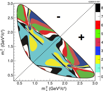
Figure 1: The equal $\Delta\delta_{D}$ binning from Ref. KzPiPiCiSi . The absolute bin number, $|i|$, is indicated by the colouring. The positive bins are defined in the region $m^{2}_{+}>m^{2}_{-}$, and the negative bins in the region $m^{2}_{+}<m^{2}_{-}$.

4.1 $K^{0}_{\rm\scriptscriptstyle S}$ veto bin

A large peaking background to $D\!\rightarrow 4\pi^{\pm}$ decays is $D\!\rightarrow K^{0}_{\rm\scriptscriptstyle S}\pi^{+}\pi^{-}$ where $K^{0}_{\rm\scriptscriptstyle S}\!\rightarrow\pi^{+}\pi^{-}$. In order to remove the majority of this background, a $K^{0}_{\rm\scriptscriptstyle S}$-veto bin is included in all $D\!\rightarrow 4\pi^{\pm}$ binning schemes that are later described in Sections 4.2 - 4.5. The region of phase space that contains any $\pi^{+}\pi^{-}$ pair satisfying $480\mathrm{\,Me\kern-1.00006ptV}<m(\pi^{+}\pi^{-})<505\mathrm{\,Me\kern-1.00006ptV}$ is designated as the $K^{0}_{\rm\scriptscriptstyle S}$-veto bin. Using the nominal $D^{0}\!\rightarrow 4\pi^{\pm}$ amplitude model, the $K^{0}_{\rm\scriptscriptstyle S}$-veto was found to remove approximately 10% of signal.

4.2 Equal / variable $\Delta\delta^{4\pi}_{\mathbf{p}}$ binning

When comparing the $K^{0}_{\rm\scriptscriptstyle S}\pi^{+}\pi^{-}$ to the $4\pi^{\pm}$ final state, one clear difference is the decay amplitudes that contribute. As discussed, $K^{0}_{\rm\scriptscriptstyle S}\pi^{+}\pi^{-}$ has contributions from both CF and DCS amplitudes, whereas $4\pi^{\pm}$ only has contributions from singly Cabibbo suppressed (SCS) amplitudes. This means that there is no clear way to divide the phase space, like the line $m^{2}_{+}=m^{2}_{-}$ in the $K^{0}_{\rm\scriptscriptstyle S}\pi^{+}\pi^{-}$ Dalitz plot. A different approach is therefore followed. The baseline amplitude model from Ref. fourpimodel is used to assign each point $\mathbf{p}$ a value of $\Delta\delta^{4\pi}_{\mathbf{p}}$, then a bin number is assigned using,

$$+i :=\forall\mathbf{p}:\phantom{-}\delta_{i-1}<\Delta\delta^{4\pi}_{\mathbf{p}}<\phantom{-}\delta_{i}$$

$$-i :=\forall\mathbf{p}:-\delta_{i-1}>\Delta\delta^{4\pi}_{\mathbf{p}}>-\delta_{i}$$ (4.1)

where $\delta_{0}\equiv 0$, $\delta_{\mathcal{N}}\equiv\pi$ and $\delta_{i}<\delta_{i+1}$. This automatically fulfils the requirement that bin $+i$ maps to bin $-i$ under $C\!P$, since $\Delta\delta^{4\pi}_{\mathbf{p}}\equiv-\Delta\delta^{4\pi}_{\mathbf{\overline{p}}}$. The values of $\delta_{i}$ are chosen using two methods: the equal $\Delta\delta^{4\pi}_{\mathbf{p}}$ binning, for which $\delta_{i}=i\pi/\mathcal{N}$; and the variable $\Delta\delta^{4\pi}_{\mathbf{p}}$ binning, for which the values of $\delta_{i}$ are chosen such that $K_{i}^{4\pi}+\bar{K}_{i}^{4\pi}$ is approximately the same in each bin.

Since amplitude models are difficult to reproduce, it is desirable to have a model-implementation-independent binning scheme. This is possible by splitting the five dimensional phase space into many small hypervolumes, each of which is assigned a bin number. The overall bin is then formed from the combination of all hypervolumes with that bin number. To create a model-implementation-independent binning scheme, referred to as a hyper-binning, a set of variables must be defined that parameterises the five-dimensional phase space of $D$ $\rightarrow$ $4\pi^{\pm}$ decays. The variables $\{m_{+},m_{-},\cos\theta_{+},\cos\theta_{-},\phi\}$ are chosen, where $m_{+}$ ($m_{-}$) is the invariant mass of the $\pi^{+}\pi^{+}$ ($\pi^{-}\pi^{-}$) pair; $\theta_{+}$ ($\theta_{-}$) is the helicity angle of the $\pi^{+}\pi^{+}$ ($\pi^{-}\pi^{-}$) pair; and $\phi$ is the angle between the $\pi^{+}\pi^{+}$ and $\pi^{-}\pi^{-}$ decay planes (a full definition of these variables can be found in Appendix A). Since the hyper-binning is most easily implemented with square phase space boundaries, the following transformation is made,

$$m_{\pm}^{\prime}=m_{\pm}+\delta\ \ \ \mathrm{where}\ \ \ \delta=\mathrm{min}\{m_{+},m_{-}\}-m_{\mathrm{min}},$$ (4.2)

where $m_{\mathrm{min}}$ is the minimum value kinematically possible for $m_{+}$ (or $m_{-}$). When using the variables $\{m_{+}^{\prime},m_{-}^{\prime},\cos\theta_{+},\cos\theta_{-},\phi\}$, the kinematically allowed region of phase space is a hypervolume defined by the corners $\{m_{\mathrm{min}}$, $m_{\mathrm{min}}$, $-1$, $-1$, $-\pi\}$ and $\{m_{\mathrm{max}}$, $m_{\mathrm{max}}$, $1$, $1$, $\pi\}$. This set of variables has been chosen to exploit the symmetries of the system, these being $C\!P$-conjugation and identical particle interchange:

$$\mathcal{CP}\{m_{+}^{\prime},m_{-}^{\prime},\cos\theta_{+},\cos\theta_{-},\phi\} \rightarrow\{m_{-}^{\prime},m_{+}^{\prime},\cos\theta_{-},\cos\theta_{+},-\phi\}$$ (4.3)

$$[\pi^{+}_{1}\leftrightarrow\pi^{+}_{2}]\{m_{+}^{\prime},m_{-}^{\prime},\cos\theta_{+},\cos\theta_{-},\phi\} \rightarrow\{m_{+}^{\prime},m_{-}^{\prime},-\cos\theta_{+},\cos\theta_{-},\phi-\pi\}$$ (4.4)

$$[\pi^{-}_{1}\leftrightarrow\pi^{-}_{2}]\{m_{+}^{\prime},m_{-}^{\prime},\cos\theta_{+},\cos\theta_{-},\phi\} \rightarrow\{m_{+}^{\prime},m_{-}^{\prime},\cos\theta_{+},-\cos\theta_{-},\phi-\pi\}$$ (4.5)

The symmetries for identical particle exchange allow the phase space to be ‘folded’ twice along the lines $\cos\theta_{+}=0$ and $\cos\theta_{-}=0$, reducing the phase space volume by a factor of four. A further folding is also possible by considering the $C\!P$ operation; for a point $\mathbf{p}$ with bin number $i$, it follows that point $\mathbf{\overline{p}}$ has bin number $-i$.

An adaptive binning algorithm is used to create a hyper-binning scheme. At the beginning of the algorithm one hypervolume is defined with corners $\{m_{\mathrm{min}}$, $m_{\mathrm{min}}$, $0$, $0$, $0\}$ and $\{m_{\mathrm{max}}$, $m_{\mathrm{max}}$, $1$, $1$, $\pi\}$. At each iteration of the algorithm, the hypervolumes from the previous iteration are split in two, choosing to split in the dimension that has the fastest varying $\Delta\delta^{4\pi}_{\mathbf{p}}$, and picking a split point that is as close as possible to one of the bin boundaries defined in Eq. 4.1. The algorithm runs until either: splitting a hypervolume will always result in two hypervolumes with the same bin number; splitting a hypervolume will always result in a hypervolume that has an edge length narrower than the minimum allowed. Several minimum edge lengths were tested and the values $\{39\mathrm{\,Me\kern-1.00006ptV},39\mathrm{\,Me\kern-1.00006ptV},0.06,0.06,0.19\rm\,rad\}$ were chosen since this results in a reasonable number of volumes ($\sim 250,000$) while reproducing the parameters $c_{i}$ and $s_{i}$ to within $2\%$ compared to a binning scheme that uses the model directly. It is possible to visualise the hyper-binning by taking two-dimensional slices of the five-dimensional phase space. Some examples are shown for the equal $\Delta\delta^{4\pi}_{\mathbf{p}}$ binning with $\mathcal{N}=5$ in Fig. 2. The full binning schemes used in this paper are provided in both ASCII and Root format as supplementary material.

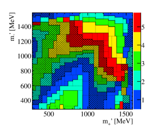
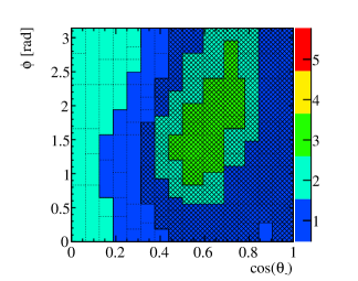
Figure 2: Two-dimensional slices of the $D\!\rightarrow 4\pi^{\pm}$ phase space showing the equal $\Delta\delta^{4\pi}_{\mathbf{p}}$ binning with $\mathcal{N}=5$. The colour denotes the absolute value of the bin number, and the cross hatching denotes a negative bin number.

4.3 Model predictions of the hadronic parameters

Using the integral expressions in Eqs. 2.2 - 2.4 it is possible to calculate the hadronic parameters for a given amplitude model and binning scheme. This is done using the baseline and alternative amplitude models given in Ref. fourpimodel . Since the baseline-model is used to determine the $D\!\rightarrow 4\pi^{\pm}$ binning schemes, using the hadronic parameters predicted with this model could result in a bias. Therefore, the arithmetic-mean of the hadronic parameters from all alternative models is used as the model prediction, and the covariance of the results is used to determine a model-uncertainty. To determine the statistical and systematic uncertainties, the hadronic parameters are calculated many times using the baseline model, each time varying the model parameters within their statistical and systematic uncertainties. The covariance of the results is used to determine a combined statistical and systematic uncertainty, which is added to the model-uncertainty in quadrature to obtain the total uncertainty. The model predictions for the equal / variable $\Delta\delta^{4\pi}_{\mathbf{p}}$ binning are shown in Fig. 3.

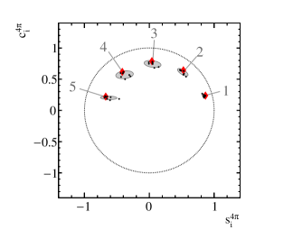
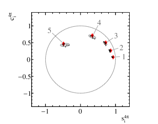
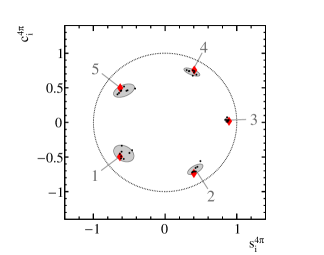
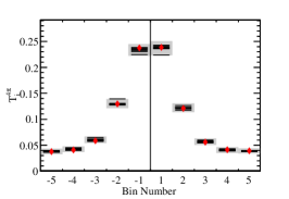
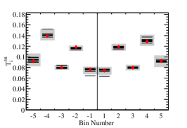
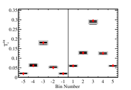
Figure 3: The model predictions of the hadronic parameters for the (left) equal $\Delta\delta^{4\pi}_{\mathbf{p}}$ binning (centre) variable $\Delta\delta^{4\pi}_{\mathbf{p}}$ binning (right) alternative binning, with $\mathcal{N}=5$. (top row) The red diamonds (black dots) show the $c_{i}^{f}$ and $s_{i}^{f}$ predictions calculated from the baseline model (alternative models). The grey shaded ellipses shows $c_{i}^{f}$ and $s_{i}^{f}$ model prediction and uncertainty as described in the text. (bottom row) The (red diamonds) black horizontal lines show the $T_{i}^{f}$ and $\bar{T}_{i}^{f}$ predictions calculated from the baseline model (alternative models). The grey shaded band shows the $T_{i}^{f}$ and $\bar{T}_{i}^{f}$ model prediction and uncertainty as described in the text.

4.4 Alternate binning

One drawback of the $\Delta\delta^{4\pi}_{\mathbf{p}}$ binning schemes is that the variation of $r^{4\pi}_{\mathbf{p}}$ across each bin is not considered, leading to $K_{i}^{f}\sim\bar{K}_{i}^{f}$, as seen in Fig. 3. This means that the interference term in the $B^{-}\!\rightarrow DK^{-}$ decay rate, given in Eq. 2.13, is relatively small in all phase space bins. Ideally, one would choose to have $r^{4\pi}_{\mathbf{p}}\ll 1$ in half of the phase space bins, enhancing the interference in these regions (and therefore the sensitivity to $\gamma$). The $r^{4\pi}_{\mathbf{p}}\ll 1$ condition is satisfied in the $K^{0}_{\rm\scriptscriptstyle S}\pi^{+}\pi^{-}$ final state, where many bins are dominated by DCS amplitudes. Although the SCS $4\pi^{\pm}$ final state has no clear line of symmetry that divides favoured from suppressed phase space regions, the amplitude model can be used to define such a split. Any point $\mathbf{p}$ that that satisfies $r^{4\pi}_{\mathbf{p}}<1$ is assigned a bin number $+i$, whereas any satisfying $r^{4\pi}_{\mathbf{p}}>1$ is assigned a bin number $-i$. The $+i$ bin numbers are assigned using,

$$+i :=\forall\mathbf{p}:\bigg{[}-\pi+\frac{2\pi}{\mathcal{N}}(i-1)<+\Delta\delta^{4\pi}_{\mathbf{p}}<-\pi+\frac{2\pi}{\mathcal{N}}i\bigg{]}\&\bigg{[}r^{4\pi}_{\mathbf{p}}>1\bigg{]},$$ (4.6)

which also uniquely defines the $-i$ bin numbers i.e.

$$-i :=\forall\mathbf{p}:\bigg{[}-\pi+\frac{2\pi}{\mathcal{N}}(i-1)<-\Delta\delta^{4\pi}_{\mathbf{p}}<-\pi+\frac{2\pi}{\mathcal{N}}i\bigg{]}\&\bigg{[}r^{4\pi}_{\mathbf{p}}<1\bigg{]}.$$ (4.7)

The same hypervolumes from the equal $\Delta\delta^{4\pi}_{\mathbf{p}}$ binning schemes are used for the alternative binning schemes, but the bin number associated to each hypervolume is reassigned using Eq. 4.6. The model predictions for the alternative binning with $\mathcal{N}=5$ is shown in Fig. 3.

4.5 Optimal binning

To determine how sensitive a binning scheme is to a measurement of $\gamma$, the $Q_{\pm}$ values are defined Bondar:2008hh ,

$$Q^{2}_{\pm}=\frac{{\sum_{i}}\left(\frac{1}{\sqrt{N_{B^{\pm}}^{i}}}\frac{\mathrm{d}N_{B^{\pm}}^{i}}{\mathrm{d}x_{\pm}}\right)^{2}+\left(\frac{1}{\sqrt{N_{B^{\pm}}^{i}}}\frac{\mathrm{d}N_{B^{\pm}}^{i}}{\mathrm{d}y_{\pm}}\right)^{2}}{{\int_{D}}\left[\left(\frac{1}{\sqrt{\Gamma_{B^{\pm}}(\mathbf{p})}}\frac{\mathrm{d}\Gamma_{B^{\pm}}(\mathbf{p})}{\mathrm{d}x_{\pm}}\right)^{2}+\left(\frac{1}{\sqrt{\Gamma_{B^{\pm}}(\mathbf{p})}}\frac{\mathrm{d}\Gamma_{B^{\pm}}(\mathbf{p})}{\mathrm{d}y_{\pm}}\right)^{2}\right]\mathrm{d}\mathbf{p}},$$ (4.8)

where $N_{B^{\pm}}^{i}$ is the number of $B^{\pm}\!\rightarrow DK^{\pm},D\!\rightarrow f$ decays expected in bin $i$ (Eq. 2.11 and Eq. 2.12), and $\Gamma_{B^{\pm}}(\mathbf{p})$ gives the differential decay rate (Eq. 2.13 and Eq. 2.14). The value of $Q_{\pm}$ gives the statistical sensitivity on the parameters $x_{\pm}$ and $y_{\pm}$ from a binned analysis of $B^{\pm}\!\rightarrow DK^{\pm},D\!\rightarrow f$ decays, divided by the statistical sensitivity from an analysis with infinitely many bins. Substituting Eqs. 2.11 - 2.14 into Eq. 4.8 gives,

$$Q^{2}_{\pm}=1-\sum_{i}\frac{K_{i}^{f}\bar{K}_{i}^{f}\left(1-(c_{i}^{f})^{2}-(s_{i}^{f})^{2}\right)}{N_{B^{\pm}}^{i}}\bigg{/}\sum_{i}K_{i}^{f}$$ (4.9)

The $Q$ value, $Q^{2}=\frac{1}{2}(Q^{2}_{+}+Q^{2}_{-})$, is then used to rank the sensitivity of different binning schemes to $\gamma$. The values $\delta_{B}=140^{\circ}$, $\gamma=70^{\circ}$ and $r_{B}=0.1$ are used to determine $Q$. For the optimisation of the $K^{0}_{\rm\scriptscriptstyle S}\pi^{+}\pi^{-}$ binning schemes in Ref. KzPiPiCiSi , a simplified $Q$ value was used where it was assumed $r_{B}=0$. Since the relative size of $K_{i}^{f}$ and $\bar{K}_{i}^{f}$ does not need to be optimised for $K^{0}_{\rm\scriptscriptstyle S}\pi^{+}\pi^{-}$ (due to the division at $m_{+}^{2}=m_{-}^{2}$), this assumption works well. For $4\pi^{\pm}$ decays, the simplified expression gives solutions where $K_{i}^{f}\sim\bar{K}_{i}^{f}$, so the full expression is used instead.

An iterative algorithm is used to take any hyper-binning scheme (i.e. a collection of hypervolumes, each with a bin number, that span the $D\!\rightarrow 4\pi^{\pm}$ phase space) and reassign the bin numbers in order to maximise the model-prediction of $Q$. Each iteration of the algorithm involves looping over every hypervolume in the hyper-binning. For each hypervolume, every possible bin number ($-\mathcal{N},...,-1,+1,+\mathcal{N}$) is assigned, and $Q$ is recalculated; the bin number that gave the largest $Q$ is then kept. The algorithm keeps running until no hypervolumes change their bin number, typically taking around $20-50$ iterations.

Since the number of free parameters being optimised is so large, it is unavoidable that the optimisation procedure will fall into a local maximum. The outcome is therefore dependent on the starting values (i.e. the bin numbers assigned to each hypervolume). The starting bin numbers are therefore assigned using two methods: the equal $\Delta\delta^{4\pi}_{\mathbf{p}}$ binning scheme (Eq. 4.1); and the alternate binning scheme (Eq. 4.6). The two sets of starting values give the ‘optimal binning’ and ‘optimal-alternative binning’, respectively. The set of hypervolumes used for the optimisation must have sufficient flexibility to describe the optimal binning. For all optimal binning schemes, the hypervolumes are first taken from the equal $\Delta\delta^{4\pi}_{\mathbf{p}}$ binning scheme with $\mathcal{N}=8$, then further divided so that, for the sample sizes used in this paper, the probability of any single hypervolume being populated is less than $1/50$.

After running the $Q$ optimisation procedure it was found that occasionally the results had very small values of $K_{i}^{f}+\bar{K}_{i}^{f}$ for one or more bin pairs. For this reason a small change was made to the optimisation metric,

$$Q^{{}^{\prime}2}=Q^{2}+\frac{1}{10}\sum_{i=1}^{\mathcal{N}}\left\{\begin{matrix}K_{i}^{f}+\bar{K}_{i}^{f}<t:&\left[\frac{K_{i}^{f}+\bar{K}_{i}^{f}-t}{t}\right]^{2}\\ K_{i}^{f}+\bar{K}_{i}^{f}>t:&0\end{matrix}\right.,$$ (4.10)

where $t=\frac{2}{3\mathcal{N}}\sum_{i=1}^{\mathcal{N}}(K_{i}^{f}+\bar{K}_{i}^{f})$ is the lower threshold at which a constraint is applied to $K_{i}^{f}+\bar{K}_{i}^{f}$.

The $Q$ value for the optimal and optimal-alternative binning schemes is shown in Fig. 4 for $\mathcal{N}=1-8$. Also shown are the $Q$ values for the other binning schemes discussed in this paper.

Figure 4: The model predictions of the $Q$ values found from all binning schemes considered in this paper. The uncertainties are found by varying the model predictions of the hadronic parameters within their uncertainties.

5 Event Selection

The data set analysed consists of $e^{+}e^{-}$ collisions produced by the Cornell Electron Storage Ring (CESR) at $\sqrt{s}=3.77$ GeV corresponding to an integrated luminosity of 818 $\rm pb^{-1}$ and collected with the CLEO-c detector. The CLEO-c detector is described in detail elsewhere CLEOREF1 ; CLEOREF2 ; CLEOREF3 ; CLEOREF4 . Monte Carlo (MC) simulated samples of signal decays are used to estimate selection efficiencies. Possible background contributions are determined from a generic $D^{0}\kern 1.99997pt\overline{\kern-1.99997ptD}{}^{0}$ simulated sample corresponding to approximately fifteen times the integrated luminosity of the data set. The EVTGEN generator EVTGEN is used to simulate the decays. The detector response is modelled using the GEANT software package GEANT .

Table 1 lists all $D$ decay final states that are reconstructed in conjunction with a $D\!\rightarrow 4\pi^{\pm}$ decay, referred to as double-tagged decays. Underlined in Tab. 1 are the $D$ decay final states that are also reconstructed alone, referred to as single-tagged decays. Unstable final state particles are reconstructed in the following decay modes: $\pi^{0}\!\rightarrow\gamma\gamma$; $K^{0}_{\rm\scriptscriptstyle S}\!\rightarrow\pi^{+}\pi^{-}$; $\omega\!\rightarrow\pi^{+}\pi^{-}\pi^{0}$; $\eta\!\rightarrow\gamma\gamma$; $\eta\!\rightarrow\pi^{+}\pi^{-}\pi^{0}$; and $\eta^{\prime}\!\rightarrow\eta(\gamma\gamma)\pi^{+}\pi^{-}$.

Type	Final States
Flavoured	$K^{\mp}e^{\pm}\nu$
Quasi-Flavoured	$\underline{K^{\mp}\pi^{\pm}}$  $K^{\mp}\pi^{\pm}\pi^{0}$ $K^{\mp}\pi^{\pm}\pi^{\mp}\pi^{\pm}$
$C\!P$ even	$\underline{K^{+}K^{-}}$  $\underline{\pi^{+}\pi^{-}}$  $\underline{K^{0}_{\rm\scriptscriptstyle S}\pi^{0}\pi^{0}}$  $K^{0}_{\rm\scriptscriptstyle L}\pi^{0}$ $K^{0}_{\rm\scriptscriptstyle L}\omega$
$C\!P$ odd	$\underline{K^{0}_{\rm\scriptscriptstyle S}\pi^{0}}$   $\underline{K^{0}_{\rm\scriptscriptstyle S}\omega}$  $\underline{K^{0}_{\rm\scriptscriptstyle S}\eta}$  $\underline{K^{0}_{\rm\scriptscriptstyle S}\eta^{\prime}}$
Self-conjugate	$K^{0}_{\rm\scriptscriptstyle S}\pi^{+}\pi^{-}$  $K^{0}_{\rm\scriptscriptstyle L}\pi^{+}\pi^{-}$  $\underline{\pi^{+}\pi^{-}\pi^{0}}$

Table 1: List of all $D$ decay final states that are reconstructed in conjunction with a $D\!\rightarrow 4\pi^{\pm}$ decay (double-tag modes). The underlined final states are also reconstructed alone (single-tag modes).

The selection procedure used for this paper is intended to be almost identical to that in Ref. FPlusFourPi . The only change is to the selection criteria used to reject peaking background from $D\!\rightarrow K^{0}_{\rm\scriptscriptstyle S}\pi^{+}\pi^{-}$ decays that are reconstructed as $D\!\rightarrow 4\pi^{\pm}$; henceforth referred to as $K^{0}_{\rm\scriptscriptstyle S}\pi^{+}\pi^{-}$ background. In Ref. FPlusFourPi any $\pi^{+}\pi^{-}$ pair with an invariant mass in the range $[0.470,0.530]\mathrm{\,Ge\kern-1.00006ptV}$ is required to have a reconstructed vertex that is compatible with the $e^{+}e^{-}$ collision point. In this paper, any $\pi^{+}\pi^{-}$ pair with an invariant mass in the range $[0.480,0.505]\mathrm{\,Ge\kern-1.00006ptV}$ is rejected, regardless of its compatibility with the $e^{+}e^{-}$ collision point. The $4\pi^{\pm}$ phase space bins defined in Sec. 4 have the same region of phase space removed, so no corrections to the measured hadronic parameters are needed. In addition to the tags in Ref. FPlusFourPi , this analysis also uses the flavour-tags $K^{\mp}e^{\pm}\nu$, and the quasi-flavour-tags $K^{\mp}\pi^{\pm}$, $K^{\mp}\pi^{\pm}\pi^{0}$ and $K^{\mp}\pi^{\pm}\pi^{\mp}\pi^{\pm}$. These decays are selected following the same criteria as Ref. KzPiPiCiSi .

The final states that do not include a neutrino or a $K^{0}_{\rm\scriptscriptstyle L}$ are fully reconstructed using the beam-constrained candidate mass, $m_{\mathrm{bc}}\equiv\sqrt{s/(4c^{4})-\mathbf{p}_{D}^{2}/c^{2}}$, where $\mathbf{p}_{D}$ is the $D$-candidate momentum, and $\Delta E\equiv E_{D}-\sqrt{s}/2$, where $E_{D}$ is the $D$-candidate energy. Requirements are first placed on the value of $\Delta E$, then $m_{\mathrm{bc}}$ is used as the discriminating variable to distinguish signal from non-peaking backgrounds. For double-tags that are dominated by background from continuum production of light quark-antiquark pairs ($\pi^{+}\pi^{-}$, $K^{+}K^{-}$, $\pi^{+}\pi^{-}\pi^{0}$ and $4\pi^{\pm}$), the signal yield is determined using an unbinned maximum likelihood fit to the average $m_{\mathrm{bc}}$ of the two $D$ decays, $m^{\mathrm{ave}}_{\mathrm{bc}}\equiv\frac{1}{2}(D_{1}\,m_{\mathrm{bc}}+D_{2}\,m_{\mathrm{bc}})$. The signal probability density function (PDF) is parameterised using the sum of a bifurcated Gaussian and a Gaussian, which have shape parameters fixed from a fit to samples of simulated signal decays. The background PDF is parameterised using an Argus function ARGUS . Figure 5 shows an example of this fit for double-tagged $\pi^{+}\pi^{-}\pi^{0}$ candidates - the signal yield is determined in the $m^{\mathrm{ave}}_{\mathrm{bc}}$ window $[1.86,1.87]\mathrm{\,Ge\kern-1.00006ptV}$. For fully-reconstructed decays that are not continuum dominated, the double-tag yield is determined by counting events in signal and sideband regions of the two dimensional $D_{1}\,m_{\mathrm{bc}}$ vs. $D_{2}\,m_{\mathrm{bc}}$ plane, as indicated in Figure 5 for double-tagged $K^{\mp}\pi^{\pm}\pi^{0}$ candidates.

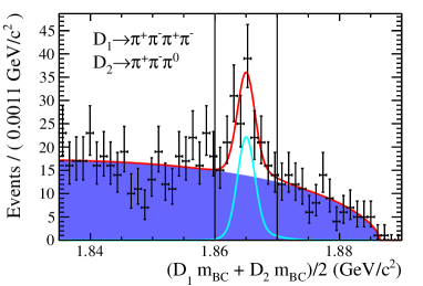
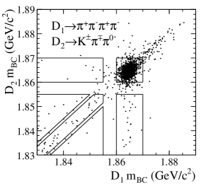
Figure 5: (left) The $m^{\mathrm{ave}}_{\mathrm{bc}}$ distribution of selected double-tagged $\pi^{+}\pi^{-}\pi^{0}$ candidates. Superimposed with a red line is the result of a unbinned maximum likelihood fit described in the text. The shaded purple area shows the background PDF, and the blue line shows the signal PDF. The vertical lines show the signal region. (right) Two dimensional $D_{1}\,m_{\mathrm{bc}}$ vs. $D_{2}\,m_{\mathrm{bc}}$ distribution of selected double tagged $K^{\mp}\pi^{\pm}\pi^{0}$ candidates. The square box covering the range $1.86-1.87\mathrm{\,Ge\kern-1.00006ptV}$ shows the signal region, and the remaining boxes show the various sideband regions that are used to determine the combinatorial background contribution.

The final states containing a neutrino or a $K^{0}_{\rm\scriptscriptstyle L}$ cannot be fully-reconstructed; the energy and momentum, $p_{\mathrm{miss}}$ and $E_{\mathrm{miss}}$, of the missing particle is inferred by using knowledge of the initial $e^{+}e^{-}$ state and conservation of energy and momentum. The missing-mass squared, $m^{2}_{\mathrm{miss}}\equiv E_{\mathrm{miss}}^{2}/c^{4}-\mathbf{p}_{\mathrm{miss}}^{2}/c^{2}$, and the quantity $U_{\mathrm{miss}}\equiv E_{\mathrm{miss}}-|\mathbf{p}_{\mathrm{miss}}|c$, are used to discriminate signal from background for decays involving a $K^{0}_{\rm\scriptscriptstyle L}$ or a neutrino, respectively. The double-tag yields are determined using an unbinned maximum likelihood fit to the discriminating variable, where the signal and background PDFs are taken from histograms of simulated data samples. Figure 6 shows an example of this fit for double-tagged $K^{\mp}e^{\pm}\nu$ and $K^{0}_{\rm\scriptscriptstyle L}\pi^{+}\pi^{-}$ candidates - the signal yields are determined within the signal windows indicated.

Figure 6: Distribution of $U_{\mathrm{miss}}$($m^{2}_{\mathrm{miss}}$) for selected double tags containing a neutrino ($K^{0}_{\rm\scriptscriptstyle L}$). Superimposed is the result of an unbinned maximum likelihood fit that is described in the text. The blue/green/red shaded area shows the distribution of combinatoric/continuum/peaking background respectively. The red line shows the total signal + background PDF. The black vertical lines indicate the events that fall within the signal region that are used for further analysis.

The dominant peaking background contribution to all double-tags is from $K^{0}_{\rm\scriptscriptstyle S}\pi^{+}\pi^{-}$ background, which is estimated from the generic MC sample of $D\kern 1.99997pt\overline{\kern-1.99997ptD}{}$ events, and typically constitutes about $5-10\%$ of the selected events. A data-driven estimate of this background is also calculated using the events that are rejected by the $\pi^{+}\pi^{-}$ mass cut - this shows good agreement with the estimates from generic MC. All decays involving a $K^{0}_{\rm\scriptscriptstyle L}$ decay have a peaking background from the equivalent decay with a $K^{0}_{\rm\scriptscriptstyle S}$ instead of a $K^{0}_{\rm\scriptscriptstyle L}$- these are referred to as cross-feed backgrounds. Using the simulated samples of $D\!\rightarrow K^{0}_{\rm\scriptscriptstyle S}X$ decays it is possible to find the ratio of $D\!\rightarrow K^{0}_{\rm\scriptscriptstyle S}X$ decays that are incorrectly reconstructed as $D\!\rightarrow K^{0}_{\rm\scriptscriptstyle L}X$ to those correctly reconstructed as $D\!\rightarrow K^{0}_{\rm\scriptscriptstyle S}X$. Since for every $D\!\rightarrow K^{0}_{\rm\scriptscriptstyle L}X$ decay considered in this paper, the equivalent $D\!\rightarrow K^{0}_{\rm\scriptscriptstyle S}X$ decay is also considered, this allows the background to be estimated using the measured $D\!\rightarrow K^{0}_{\rm\scriptscriptstyle S}X$ yields. The decay $\pi^{+}\pi^{-}\pi^{0}$ has a peaking background from $K^{0}_{\rm\scriptscriptstyle S}\pi^{0}$ that is largely suppressed by requiring the $\pi^{+}\pi^{-}$ vertex to be consistent with with $e^{+}e^{-}$ collision point. Since the decay $K^{0}_{\rm\scriptscriptstyle S}\pi^{0}$ is also considered in this paper, the $K^{0}_{\rm\scriptscriptstyle S}\pi^{0}$ signal yield can be used (in the same manner as for the cross-feed backgrounds) to estimate the background contribution. All remaining peaking backgrounds are either negligible, or considered in the systematics uncertainties in Sec. 7.

Single-tagged candidates are selected using identical criteria to the corresponding double tags, with the exception of $\pi^{+}\pi^{-}$, $K^{+}K^{-}$ and $K^{\mp}\pi^{\pm}$ decays that have additional cuts to veto cosmic ray muon and radiative Bhabha events FPlusPiPiPiz . The number of single-tags is estimated from a fit to the $m_{\mathrm{bc}}$ distribution. The signal and background PDFs are the same as those used in the fit to the $m^{\mathrm{ave}}_{\mathrm{bc}}$ distribution of continuum dominated double-tags. The signal shape parameters are fixed from a sample of simulated signal decays. Figure 7 shows an example of this fit for single-tagged $\pi^{+}\pi^{-}\pi^{0}$ candidates - the signal yield is determined in the signal region indicated. Following Ref. FPlusPiPiPiz , a further uncertainty is assigned to each of the single-tag yields to account for any mismodelling of the signal PDF. For final states with no electromagnetically neutral final state particles ($K^{+}K^{-}$, $\pi^{+}\pi^{-}$, $K^{\mp}\pi^{\pm}$) the uncertainty assigned is 2.0% of the measured signal yield. For final states where the neutrals are relatively hard ($K^{0}_{\rm\scriptscriptstyle S}\pi^{0}$, $K^{0}_{\rm\scriptscriptstyle S}\eta(\gamma\gamma)$) or soft (all other modes), uncertainties of 2.5% and 5.0% are assigned, respectively.

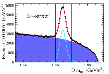
Figure 7: The $m_{\mathrm{bc}}$ distribution of selected $\pi^{+}\pi^{-}\pi^{0}$ single tagged candidates. Superimposed with a red line is the result of a unbinned maximum likelihood fit described in the text. The shaded purple area shows the background PDF, and the blue line shows the signal PDF. The vertical lines show the signal region.

In events where more than one single- or double-tagged candidate is reconstructed, an algorithm is used to select a single candidate based on information provided by the $\Delta E$ and $m_{\mathrm{bc}}$ variables. The particular choice of metric varies depending on the category of double-tag, and is optimised through simulation studies.

Decay Mode	$\pi^{+}\pi^{-}\pi^{+}\pi^{-}$	All
$K^{+}K^{-}$	$18.2\pm 6.5$	$11887.5\pm 318.8$
$\pi^{+}\pi^{-}$	$3.0\pm 8.3$	$5599.5\pm 170.8$
$K^{0}_{S}\pi^{0}\pi^{0}$	$18.2\pm 5.6$	$6989.7\pm 374.1$
$K^{0}_{L}\pi^{0}$	$41.6\pm 10.6$	–
$K^{0}_{L}\omega$	$23.4\pm 6.7$	–
$K^{0}_{S}\pi^{0}$	$111.1\pm 11.1$	$19984.0\pm 520.8$
$K^{0}_{S}\omega$	$47.4\pm 7.3$	$8033.6\pm 413.3$
$K^{0}_{S}\eta(\gamma\gamma)$	$18.9\pm 4.6$	$2903.7\pm 99.1$
$K^{0}_{S}\eta(\pi^{+}\pi^{-}\pi^{0})$	$6.7\pm 2.7$	$1283.2\pm 80.3$
$K^{0}_{S}\eta^{{}^{\prime}}$	$7.6\pm 2.9$	$1321.9\pm 76.6$
$K^{0}_{L}\pi^{+}\pi^{-}$	$488.0\pm 27.1$	–
$K^{0}_{S}\pi^{+}\pi^{-}$	$237.4\pm 16.6$	–
$\pi^{+}\pi^{-}\pi^{0}$	$63.1\pm 14.1$	$30032.4\pm 1553.9$
$K^{\pm}e^{\mp}\nu$	$484.5\pm 22.1$	–
$K^{\pm}\pi^{\mp}$	$595.6\pm 24.7$	$131613.0\pm 2658.1$
$K^{\pm}\pi^{\mp}\pi^{0}$	$1243.4\pm 36.5$	–
$K^{\pm}\pi^{\mp}\pi^{\pm}\pi^{\mp}$	$923.7\pm 41.2$	–

Table 2: Number of selected single- and double-tagged decays after background subtraction.

For double-tagged decays, the signal yields are evaluated in bins of $4\pi^{\pm}$, $K^{0}_{\rm\scriptscriptstyle S}\pi^{+}\pi^{-}$ and $K^{0}_{\rm\scriptscriptstyle L}\pi^{+}\pi^{-}$ phase space. For these final states, the four-momenta of the $D$ daughters are determined with a constraint on the previously measured $D^{0}$ mass PDG2014 , ensuring that all signal candidates fall within the kinematically allowed region of phase space. The $4\pi^{\pm}$ final state is binned using the schemes in Sec. 4. The $K^{0}_{\rm\scriptscriptstyle S}\pi^{+}\pi^{-}$ and $K^{0}_{\rm\scriptscriptstyle L}\pi^{+}\pi^{-}$ final states are binned according to the ‘Equal $\Delta\delta_{D}$ BABAR 2008’ scheme from Ref. KzPiPiCiSi , which is shown in Fig. 1. For non-continuum dominated decays, the binned yields are determined by counting the number of candidates in the signal region of the $D_{1}\,m_{\mathrm{bc}}$ vs. $D_{2}\,m_{\mathrm{bc}}$ plane - the background estimates are discussed in Sec. 6. For continuum-dominated final states a fit the $m^{\mathrm{ave}}_{\mathrm{bc}}$ distribution is performed in each phase space bin. In the case where 2 or more phase space bins have an identical decay rate (e.g. $4\pi^{\pm}$ vs. $\pi^{+}\pi^{-}\pi^{0}$ has the same decay rate in bin $+i$ and $-i$) they are merged before determining the signal yield. The samples of flavour and quasi-flavour double-tags are split using the charge of the kaon before the binned yields are determined. The phase space-integrated background subtracted event yields for all single- and double-tagged decays are given in Tab. 2.

6 Fit for $4\pi^{\pm}$ hadronic parameters

This section describes the fitting algorithm used to determine constraints on the $D\!\rightarrow 4\pi^{\pm}$ hadronic parameters. Following from Eq. 2.7, the expected number of $\psi(3770)\rightarrow D\kern 1.99997pt\overline{\kern-1.99997ptD}{}\rightarrow f_{i}g_{j}$ signal decays is given by,

$$N^{\mathrm{sig}}_{f_{i}g_{j}}=$$

$$N_{D\kern 1.39998pt\overline{\kern-1.39998ptD}{}}\bigg{\{} \left(1+\frac{y_{D}^{2}-x_{D}^{2}}{2}\right)\left[K_{i}^{f}\bar{K}_{j}^{g}+\bar{K}_{i}^{f}K_{j}^{g}-2\sqrt{K_{i}^{f}\bar{K}_{j}^{g}\bar{K}_{i}^{f}K_{j}^{g}}\left(c_{i}^{f}c_{j}^{g}+s_{i}^{f}s_{j}^{g}\right)\right]$$

$$+ \left(\phantom{1+\ }\frac{y_{D}^{2}+x_{D}^{2}}{2}\right)\left[K_{i}^{f}K_{j}^{g}+\bar{K}_{i}^{f}\bar{K}_{j}^{g}-2\sqrt{K_{i}^{f}\bar{K}_{j}^{g}\bar{K}_{i}^{f}K_{j}^{g}}\left(c_{i}^{f}c_{j}^{g}-s_{i}^{f}s_{j}^{g}\right)\right]\bigg{\}}$$ (6.1)

where $N_{D\kern 1.39998pt\overline{\kern-1.39998ptD}{}}$ is the total number of $\psi(3770)\rightarrow D\kern 1.99997pt\overline{\kern-1.99997ptD}{}$ decays in the data sample. In the literature, different parameterisations of the hadronic parameters are used for different categories of final state, which sometimes differ from $K_{i}^{f}$, $\bar{K}_{i}^{f}$, $c_{i}^{f}$ and $s_{i}^{f}$ parameterisation used to derive the formalism in this paper. The different parameterisations used are summarised in Tab. 3, which are used as free parameters in the fit for the relevant final states. The new parameters introduced are: the $C\!P$-even fraction, $F_{+}^{f}$; the coherence factor, $R_{D}^{f}$; the average strong phase difference, $\delta_{D}^{f}$; and the ratio of $\kern 1.99997pt\overline{\kern-1.99997ptD}{}^{0}\!\rightarrow f$ to $D^{0}\!\rightarrow f$ amplitudes, $r_{D}^{f}$. The relationship between these and the $K_{i}^{f}$, $\bar{K}_{i}^{f}$, $c_{i}^{f}$ and $s_{i}^{f}$ parameters is given in Tab. 3.

Type	$K_{i}^{f}$	$\bar{K}_{i}^{f}$	$c_{i}^{f}$	$s_{i}^{f}$
$D^{0}$ flavour tag	$\mathrm{BF}(D^{0}\!\rightarrow f)$	0	0	0
$D^{0}$ quasi-flavour tag	$\mathrm{BF}(D^{0}\!\rightarrow f)$	$\mathrm{BF}(D^{0}\!\rightarrow f)(r_{D}^{f})^{2}$	$R_{D}^{f}\cos\delta_{D}^{f}$	$R_{D}^{f}\sin\delta_{D}^{f}$
$C\!P$ tag	$\mathrm{BF}(D^{0}\!\rightarrow f)$	$\mathrm{BF}(D^{0}\!\rightarrow f)$	$\eta_{C\!P}$	0
Self-conjugate tag	$\mathrm{BF}(D^{0}\!\rightarrow f)$	$\mathrm{BF}(D^{0}\!\rightarrow f)$	$2F^{f}_{+}-1$	0
$4\pi^{\pm}$/ $K^{0}_{S/L}\pi\pi$	$K_{i}^{f}$	$\bar{K}_{i}^{f}$	$c_{i}^{f}$	$s_{i}^{f}$
All $D$ decay final states	1	1	$y_{D}$	0

Table 3: List of the different parameterisations used for the hadronic parameters of different categories of final state, and how they relate the $K_{i}^{f}$, $\bar{K}_{i}^{f}$, $c_{i}^{f}$ and $s_{i}^{f}$ parameterisation used to derive the formalism in this paper.

Substituting the various parameterisations in Tab. 3 into Eq. 6.1, it is clear that different categories of tag provide sensitivity to different hadronic parameters. The flavour and quasi-flavour tags give sensitivity to $K_{i}^{f}$ and $\bar{K}_{i}^{f}$; the $C\!P$ tags and $\pi^{+}\pi^{-}\pi^{0}$ tags give sensitivity to $K_{i}^{f}$, $\bar{K}_{i}^{f}$, and $c_{i}^{f}$; and the $K^{0}_{\rm\scriptscriptstyle S}\pi^{+}\pi^{-}$ and $K^{0}_{\rm\scriptscriptstyle L}\pi^{+}\pi^{-}$ tags give sensitivity to all hadronic parameters.

The expected efficiency and background corrected yield is given by,

$$N^{\mathrm{tot}}_{f_{i}g_{j}}=N^{\mathrm{sig}}_{f_{i}g_{j}}\epsilon_{f_{i}g_{j}}+N^{\mathrm{bkg}}_{f_{i}g_{j}}$$ (6.2)

where $\epsilon_{f_{i}g_{j}}$ is the reconstruction and selection efficiency for the decay in question, and $N^{\mathrm{bkg}}_{f_{i}g_{j}}$ is the expected number of background. The quantity $\epsilon_{f_{i}g_{j}}$ is determined from large samples of simulated signal decays, correcting for known discrepancies between data and simulation. Before efficiencies are calculated, the simulated samples containing $K^{0}_{\rm\scriptscriptstyle S}\pi^{+}\pi^{-}$ and $4\pi^{\pm}$ decays are reweighted to their model expectations (using the $D^{0}\!\rightarrow K^{0}_{\rm\scriptscriptstyle S}\pi^{+}\pi^{-}$ BABAR model BABAR2008 and the nominal $D^{0}\!\rightarrow 4\pi^{\pm}$ model fourpimodel ) including the effects of quantum correlations. The simulated sample of $K^{0}_{\rm\scriptscriptstyle L}\pi^{+}\pi^{-}$ decays is also reweighted to the $K^{0}_{\rm\scriptscriptstyle S}\pi^{+}\pi^{-}$ model with $\Delta\delta^{K^{0}_{\rm\scriptscriptstyle L}\pi\pi}_{\mathbf{p}}=-\Delta\delta^{K^{0}_{\rm\scriptscriptstyle S}\pi\pi}_{\mathbf{p}}$; this approximation holds in the scenario that only CF and DCS amplitudes contribute, and the two do not overlap in the Dalitz plot. A systematic uncertainty is later assigned to account for any model dependence in the efficiency determination.

The total background estimate is broken down into the following expression,

$$N^{\mathrm{bkg}}_{f_{i}g_{j}}=N^{K^{0}_{\rm\scriptscriptstyle S}\pi\pi}_{fg}\kappa^{K^{0}_{\rm\scriptscriptstyle S}\pi\pi}_{f_{i}g_{j}}+N^{\mathrm{flat}}_{fg}\kappa^{\mathrm{flat}}_{f_{i}g_{j}}+N^{\mathrm{sig}}_{f_{i}h_{j}}\epsilon_{f_{i}h_{j}}f^{h}_{g}$$ (6.3)

where $N^{K^{0}_{\rm\scriptscriptstyle S}\pi\pi}_{fg}$ and $N^{\mathrm{flat}}_{fg}$ are the total number of $K^{0}_{\rm\scriptscriptstyle S}\pi^{+}\pi^{-}$ and combinatoric background in the $D\kern 1.99997pt\overline{\kern-1.99997ptD}{}\rightarrow fg$ decay, respectively. The quantities $\kappa^{K^{0}_{\rm\scriptscriptstyle S}\pi\pi}_{f_{i}g_{j}}$ and $\kappa^{\mathrm{flat}}_{f_{i}g_{j}}$ give the fraction of background that falls into the phase space bins $i$ and $j$. The final term, $N^{\mathrm{sig}}_{f_{i}h_{j}}\epsilon_{f_{i}h_{j}}f^{h}_{g}$, gives the number of cross-feed background from the decay $D\kern 1.99997pt\overline{\kern-1.99997ptD}{}\!\rightarrow f_{i}h_{j}$. The quantity $f^{h}_{g}$ gives the fraction of $D\kern 1.99997pt\overline{\kern-1.99997ptD}{}\!\rightarrow f_{i}h_{j}$ decays that are incorrectly reconstructed as $D\kern 1.99997pt\overline{\kern-1.99997ptD}{}\!\rightarrow f_{i}g_{j}$, to those correctly reconstructed. The value of $N^{K^{0}_{\rm\scriptscriptstyle S}\pi\pi}_{fg}$ is taken from generic MC, as was used for the determination of the of background subtracted yields in Tab. 2. The value of $\kappa^{K^{0}_{\rm\scriptscriptstyle S}\pi\pi}_{f_{i}g_{j}}$ is found using a large sample of simulated $D\!\rightarrow K^{0}_{\rm\scriptscriptstyle S}\pi^{+}\pi^{-}$ decays that are reconstructed as $D\!\rightarrow 4\pi^{\pm}$. Before calculating $\kappa^{K^{0}_{\rm\scriptscriptstyle S}\pi\pi}_{f_{i}g_{j}}$, the simulated sample is first reweighted to the model expectation, based on the phase space location of the generated $K^{0}_{\rm\scriptscriptstyle S}\pi^{+}\pi^{-}$ decay, and including quantum correlations. Since the $K^{0}_{\rm\scriptscriptstyle S}\pi^{+}\pi^{-}$ model has been shown to give good agreement with model-independent measurements KzPiPiCiSi , any model dependent bias should be small, but this is considered as a systematic uncertainty later. The value of $N^{\mathrm{flat}}_{fg}$ is determined from the sideband regions, as described in Sec. 5. For continuum-dominated and single-tagged decays $N^{\mathrm{flat}}_{fg}=0$, since the signal yields are determined from a fit to $m^{\mathrm{ave}}_{\mathrm{bc}}$, so already have the combinatoric background component subtracted. The value of $\kappa^{\mathrm{flat}}_{f_{i}g_{j}}$ is determined using simulated signal decays distributed according to the density of states (phase space). Where possible, this assumption is checked using the sideband regions, which shows good agreement. Systematic uncertainties are assigned to cover any bias from this assumption.

The values of the $4\pi^{\pm}$ hadronic parameters are obtained by maximising the log-likelihood, $\log\mathcal{L}$. The Poisson distribution, $P(k;\lambda)\equiv\lambda^{k}e^{-\lambda}/k!$, gives the probability of observing $k$ events when $\lambda$ are expected. For double-tagged decays that are not continuum-dominated the log-likelihood receives a term,

$$\log\mathcal{L}\mathrel{{+}{=}}\log P(M_{f_{i}g_{j}};N^{\mathrm{tot}}_{f_{i}g_{j}}),$$ (6.4)

where $M_{f_{i}g_{j}}$ is the number of events counted in the signal region of the decay $D\kern 1.99997pt\overline{\kern-1.99997ptD}{}\rightarrow f_{i}g_{j}$. For continuum-dominated double-tags and single-tags, the signal yield is obtained from a fit, which has an associated uncertainty $\sigma_{f_{i}g_{j}}$. Therefore, the log-likelihood receives a term,

$$\log\mathcal{L}\mathrel{{+}{=}}\log G(N^{\mathrm{tot}}_{f_{i}g_{j}};M_{f_{i}g_{j}},\sigma_{f_{i}g_{j}})$$ (6.5)

where $G(k;\mu,\sigma)$ is a Gaussian distribution with mean $\mu$ and width $\sigma$.

External inputs are needed to constrain various parameters in the fit. For the partially-reconstructed $C\!P$ final states $K^{0}_{\rm\scriptscriptstyle L}\pi^{0}$ and $K^{0}_{\rm\scriptscriptstyle L}\omega$ it is not possible to obtain a single-tagged sample, which would provide the fitter with constraints on the product $N_{D\kern 1.39998pt\overline{\kern-1.39998ptD}{}}\times\mathrm{BF}(D^{0}\rightarrow f)$. This constraint is important for normalising the respective double-tag yield, so an alternative method is followed for the $K^{0}_{\rm\scriptscriptstyle L}\pi^{0}$ and $K^{0}_{\rm\scriptscriptstyle L}\omega$ final states. In order to constrain $N_{D\kern 1.39998pt\overline{\kern-1.39998ptD}{}}$, the single-tagged $K^{\mp}\pi^{\pm}$ yield is measured in conjunction with an external constraint on $\mathrm{BF}(D^{0}\rightarrow K^{\mp}\pi^{\pm})$ PDG2014 . External constraints on $\mathrm{BF}(D^{0}\rightarrow K^{0}_{\rm\scriptscriptstyle L}\pi^{0})$ and $\mathrm{BF}(D^{0}\rightarrow K^{0}_{\rm\scriptscriptstyle L}\omega)$ then lead to the desired constraint on $N_{D\kern 1.39998pt\overline{\kern-1.39998ptD}{}}\times\mathrm{BF}(D^{0}\rightarrow f)$ PDG2014 . For the quasi-flavour tags, external constraints are provided for the hadronic parameters $r_{D}^{f}$, $R_{D}^{f}$ and $\delta_{D}^{f}$, which are taken from Ref. HFAGCKM2016 and Ref. LHCbCLEOComb . The self-conjugate final state $\pi^{+}\pi^{-}\pi^{0}$ is not a $C\!P$ eigenstate, so its $C\!P$-even fraction, $F^{\pi\pi\pi^{0}}_{+}$, is constrained to its previously measured value FPlusFourPi . The charm-mixing parameters are constrained to their world-average values HFAGCKM2016 . The central values and uncertainties of the constraints are listed in Tab. 4. All constraints are applied by including a Gaussian constraint, similar to Eq. 6.5, in the $\log\mathcal{L}$; where available, correlations between the parameters are also included.

Fit Parameter	Constraint	Source
$\mathrm{BF}(D^{0}\rightarrow K^{-}\pi^{+})$	(3.93 $\pm$ 0.04)%	Ref. PDG2014 *
$\mathrm{BF}(D^{0}\rightarrow K^{0}_{\rm\scriptscriptstyle L}\pi^{0})$	(1.00 $\pm$ 0.07)%
$\mathrm{BF}(D^{0}\rightarrow K^{0}_{\rm\scriptscriptstyle L}\omega(3\pi))$	(0.99 $\pm$ 0.05 $\pm$ 0.20)%
$r^{K^{-}\pi^{+}}$	(5.90 $\pm$ 0.03)%	Ref. HFAGCKM2016 $\dagger$
$\delta^{K^{-}\pi^{+}}$	3.41 $\pm$ 0.14
$r^{K^{-}\pi^{+}\pi^{0}}$	(4.47 $\pm$ 0.12)%	Ref. LHCbCLEOComb
$R^{K^{-}\pi^{+}\pi^{0}}$	0.81 $\pm$ 0.06
$\delta^{K^{-}\pi^{+}\pi^{0}}$	3.46 $\pm$ 0.25
$r^{K^{-}3\pi}$	(5.49 $\pm$ 0.06)%
$R^{K^{-}3\pi}$	0.43 $\pm$ 0.15
$\delta^{K^{-}3\pi}$	2.23 $\pm$ 0.39
$x_{D}$	(0.322 $\pm$ 0.140)%	Ref. HFAGCKM2016
$y_{D}$	(0.688 $\pm$ 0.060)%
$F^{\pi\pi\pi^{0}}_{+}$	0.973 $\pm$ 0.017	Ref. FPlusFourPi
*The constraint on $\mathrm{BF}(D^{0}\rightarrow K^{0}_{\rm\scriptscriptstyle L}\omega(3\pi))$ is taken from $\mathrm{BF}(D^{0}\rightarrow K^{0}_{\rm\scriptscriptstyle S}\omega(3\pi))$ with a systematic uncertainty of 20%.
$\dagger$Ref. HFAGCKM2016 uses the convention $C\!P|D^{0}\rangle=-|\kern 1.59998pt\overline{\kern-1.59998ptD}{}^{0}\rangle$, so the transformation $\delta^{K^{-}\pi^{+}}\rightarrow\delta^{K^{-}\pi^{+}}+\pi$ is applied.

Table 4: List constraints used in the analysis. The right hand column gives the source of the constraint, along with any conventional adjustments that have to be made to use them in this analysis.

The hadronic parameters of the $K^{0}_{\rm\scriptscriptstyle S}\pi^{+}\pi^{-}$ and $K^{0}_{\rm\scriptscriptstyle L}\pi^{+}\pi^{-}$ final states are also constrained. The parameters $c_{i}^{K^{0}_{\rm\scriptscriptstyle S}\pi\pi}$, $s_{i}^{K^{0}_{\rm\scriptscriptstyle S}\pi\pi}$, $c_{i}^{K^{0}_{\rm\scriptscriptstyle L}\pi\pi}$ and $s_{i}^{K^{0}_{\rm\scriptscriptstyle L}\pi\pi}$ are constrained using the covariance matrix for the BABAR equal $\Delta\delta_{D}$ binning given in Ref. KzPiPiCiSi . An adjustment must be made to the constraints on $c_{i}^{K^{0}_{\rm\scriptscriptstyle L}\pi\pi}$ and $s_{i}^{K^{0}_{\rm\scriptscriptstyle L}\pi\pi}$, since a different convention is used in Ref. KzPiPiCiSi such that $c_{i}^{K^{0}_{\rm\scriptscriptstyle L}\pi\pi}\rightarrow-c_{i}^{K^{0}_{\rm\scriptscriptstyle L}\pi\pi}$ and $s_{i}^{K^{0}_{\rm\scriptscriptstyle L}\pi\pi}\rightarrow-s_{i}^{K^{0}_{\rm\scriptscriptstyle L}\pi\pi}$. Constraints on the parameters $F_{i}^{K^{0}_{\rm\scriptscriptstyle L}\pi\pi}$ and $\bar{F}_{i}^{K^{0}_{\rm\scriptscriptstyle L}\pi\pi}$ are taken directly from Ref. BrisbaneThesis ; since it is the parameters $K_{i}^{K^{0}_{\rm\scriptscriptstyle L}\pi\pi}$ and $\bar{K}_{i}^{K^{0}_{\rm\scriptscriptstyle L}\pi\pi}$ that are used as free parameters in the fit, $F_{i}^{K^{0}_{\rm\scriptscriptstyle L}\pi\pi}$ and $\bar{F}_{i}^{K^{0}_{\rm\scriptscriptstyle L}\pi\pi}$ are calculated dynamically so that the constraint can be applied. The parameters $F_{i}^{K^{0}_{\rm\scriptscriptstyle S}\pi\pi}$ and $\bar{F}_{i}^{K^{0}_{\rm\scriptscriptstyle S}\pi\pi}$ are constrained from an average of BELLE and BABAR model predictions BELLEModel ; BABARModel , as determined in Ref. newCoherenceCLEO . Since the amplitude models are fit to $D$ decay-time integrated samples of $D^{*+}\!\rightarrow D^{0}\pi^{+}$ decays, small corrections must be made for $D$-mixing using the expression K3piLHCb ,

$$B_{i}^{K^{0}_{\rm\scriptscriptstyle S}\pi\pi}\propto F_{i}^{K^{0}_{\rm\scriptscriptstyle S}\pi\pi}-\sqrt{F_{i}^{K^{0}_{\rm\scriptscriptstyle S}\pi\pi}\bar{F}_{i}^{K^{0}_{\rm\scriptscriptstyle S}\pi\pi}}(c_{i}^{K^{0}_{\rm\scriptscriptstyle S}\pi\pi}y_{D}+s_{i}^{K^{0}_{\rm\scriptscriptstyle S}\pi\pi}x_{D})+\frac{x_{D}^{2}+y_{D}^{2}}{2},$$ (6.6)

where $B_{i}^{K^{0}_{\rm\scriptscriptstyle S}\pi\pi}$ is the fraction of $D^{*+}\rightarrow D^{0}\pi^{+},D^{0}\!\rightarrow K^{0}_{\rm\scriptscriptstyle S}\pi^{+}\pi^{-}$ decays in phase space bin $i$. Using external inputs from Refs. KzPiPiCiSi ; HFAGCKM2016 , the system of equations is solved to find $F_{i}^{K^{0}_{\rm\scriptscriptstyle S}\pi\pi}$ and $\bar{F}_{i}^{K^{0}_{\rm\scriptscriptstyle S}\pi\pi}$.

In principle, the normalisation parameter $N_{D\kern 1.39998pt\overline{\kern-1.39998ptD}{}}$ can be shared for every decay mode considered in the analysis, since the same $e^{+}e^{-}$ collision data are used. In reality, however, this is not always desirable since the estimation of $N_{D\kern 1.39998pt\overline{\kern-1.39998ptD}{}}$ relies on the absolute efficiencies (rather than the relative, bin-to-bin, efficiencies) determined from simulated samples. For the double-tagged samples of $K^{0}_{\rm\scriptscriptstyle S}\pi^{+}\pi^{-}$, $K^{0}_{\rm\scriptscriptstyle L}\pi^{+}\pi^{-}$, $K^{\mp}\pi^{\pm}\pi^{0}$, $K^{\mp}\pi^{\pm}\pi^{\mp}\pi^{\pm}$, and $K^{\mp}e^{\pm}\nu$ decays, almost all information comes from the relative bin-to-bin yields, so sharing a normalisation parameter provides little benefit while introducing a potential source of systematic uncertainty. Therefore, these final states each have their own normalisation parameter, $N_{D\kern 1.39998pt\overline{\kern-1.39998ptD}{}}^{f}$, in the fit. On the other hand, the double- and single-tagged $K^{\mp}\pi^{\pm}$ samples share a normalisation constant, which allows the fitter to constrain $\mathrm{BF}(D^{0}\!\rightarrow 4\pi^{\pm})$, since $\mathrm{BF}(D^{0}\!\rightarrow K^{-}\pi^{+})$ has an external constraint (Tab. 4). This normalisation constant is also shared with all single- and double-tagged $C\!P$ and $\pi^{+}\pi^{-}\pi^{0}$ final states.

The $\log\mathcal{L}$ expression is maximised numerically using the MINUIT software MINUIT . The maximisation procedure is repeated 5 times with different starting values to ensure the global maximum of $\log\mathcal{L}$ has been found (as opposed to a local maximum). Statistical uncertainties and correlations between fit parameters are provided by Minuit from evaluating the second derivatives of $\log\mathcal{L}$ with respect to the fit parameters.

The fitting procedure is tested using 400 simulated experiments that use the background and efficiency estimates from the fit to data. The $D\!\rightarrow 4\pi^{\pm}$ hadronic parameters used to generated the pseudo-experiments are taken from model predictions. The hadronic parameters of other final states are taken from their previously measured values, and randomly sampled from their associated uncertainties. No statistically significant bias was found in the fit procedure.

The central values and statistical uncertainties of the $D\!\rightarrow 4\pi^{\pm}$ hadronic parameters from the fit to data are given in Tab. 7, and the statistical correlations in Appendix B. In this paper only results using $4\pi^{\pm}$ binning schemes with $\mathcal{N}=5$ are presented, although the results for $\mathcal{N}=1-5$ can be found in the supplementary material.

7 Systematics

The systematic uncertainties on the $4\pi^{\pm}$ hadronic parameters are broken down into several components, as listed in the systematic uncertainty breakdown in Tab. 5. Each of these components will be discussed in the following.

Bin migration

Due to the finite detector resolution, it is possible for an event occurring in one phase space bin to be reconstructed in another; this bin-migration is relevant to the $4\pi^{\pm}$, $K^{0}_{\rm\scriptscriptstyle S}\pi^{+}\pi^{-}$ and $K^{0}_{\rm\scriptscriptstyle L}\pi^{+}\pi^{-}$ final states. Since decays to these final states do not proceed by any narrow resonances, bin migration is not expected to significantly bias the result. Using samples of simulated signal events (that are reweighted to their model expectations), a migration matrix is calculated, whose elements $M_{ik}$ give the probably of an event generated in bin $k$ to be reconstructed in bin $i$. For the fully-reconstructed final states $4\pi^{\pm}$ and $K^{0}_{\rm\scriptscriptstyle S}\pi^{+}\pi^{-}$, the diagonal elements of $M_{ik}$ are typically $\sim 95\%$, whereas for the partially reconstructed $K^{0}_{\rm\scriptscriptstyle L}\pi^{+}\pi^{-}$ final state they are $\sim 85\%$. The migration matrices are used in the calculation of the expected yields (Eq. 6.2) and the fit is rerun. The absolute difference between this result and the nominal result, which is obtained without correcting for bin-migration, is taken as a systematic uncertainty.

Multiple candidate selection

To check that the multiple candidate selection (MCS) procedure does not bias the result, an alternative MCS procedure is followed where one candidate is chosen at random (rather than based on a metric). The difference between the hadronic parameters determined using this selection and the nominal selection is taken as a systematic uncertainty.

Relative efficiencies

In the nominal fit, the relative efficiency between phase space bins is determined using simulated signal samples that are reweighted to their model expectation. To estimate an upper limit on the systematic uncertainty introduced by the model uncertainty, the efficiency estimates are redetermined with the simulated samples reweighted to phase space. The absolute difference between the result using alternative efficiency estimates and the nominal result is taken as a systematic uncertainty.

Relative $K^{0}_{\rm\scriptscriptstyle S}\pi^{+}\pi^{-}$ background distribution

To determine the relative distribution of $K^{0}_{\rm\scriptscriptstyle S}\pi^{+}\pi^{-}$ background, a sample of simulated $D\!\rightarrow K^{0}_{\rm\scriptscriptstyle S}\pi^{+}\pi^{-}$ decays, reconstructed as $D\!\rightarrow 4\pi^{\pm}$, is reweighted to its model prediction, including quantum correlations. In order to determine a systematic uncertainty, the quantum correlations are neglected (equivalent to setting $c_{i}^{f}=s_{i}^{f}=0$ in Eq. 6.1) and the $K^{0}_{\rm\scriptscriptstyle S}\pi^{+}\pi^{-}$ background distribution is recalculated. The absolute difference between this result and the nominal result is taken as a systematic uncertainty.

Absolute $K^{0}_{\rm\scriptscriptstyle S}\pi^{+}\pi^{-}$ background yields

In the nominal fit, the total number of $K^{0}_{\rm\scriptscriptstyle S}\pi^{+}\pi^{-}$ background events are estimated using the generic sample of simulated data. Alternatively, this is determined using a data-driven technique. The relative event numbers in the $K^{0}_{\rm\scriptscriptstyle S}$ veto region and the signal region is determined from simulation for both $K^{0}_{\rm\scriptscriptstyle S}\pi^{+}\pi^{-}$ background and $4\pi^{\pm}$ signal. These numbers are used to estimate the $K^{0}_{\rm\scriptscriptstyle S}\pi^{+}\pi^{-}$ background contamination in the signal region based on the observed number of events in the $K^{0}_{\rm\scriptscriptstyle S}$ veto region. The fit is rerun with the alternative $K^{0}_{\rm\scriptscriptstyle S}\pi^{+}\pi^{-}$ background yields, and the absolute difference between this result and the nominal result is taken as a systematic uncertainty.

Relative flat background distribution

The relative number of combinatorial background events across phase space bins is assumed to be distributed according to phase space. As an alternative method, the relative numbers are taken from the combinatorial background events in the generic MC sample. The absolute difference between this result and the nominal result is taken as a systematic uncertainty.

Absolute flat background yields

For fully-reconstructed non-continuum dominated double-tagged decays, the total number of combinatorial background is estimated from the number of events in five sideband regions of the two dimensional $D_{1}\,m_{\mathrm{bc}}$ vs. $D_{2}\,m_{\mathrm{bc}}$ plane (see Fig. 5). Each sideband region is associated with a particular background type, which is assumed to have the same density in the sideband and signal regions. Alternatively, the relative density of background between the sideband and signal regions is taken from generic MC. The alternative background estimates are used in the fit, and the difference between this result and the nominal result is taken as a systematic uncertainty.

For partially-reconstructed double-tagged decays, the total number of combinatorial background is determined from a fit to the $m^{2}_{\mathrm{miss}}$ or $U_{\mathrm{miss}}$ distribution (see Fig. 6). Alternatively, the combinatorial background yield is determined using a simpler sideband-subtraction approach. The alternative background estimates are used in the fit, and the difference between this result and the nominal result is taken as a systematic uncertainty.

Continuum dominated signal yields

For continuum-dominated double-tagged decays, the signal yield in each phase space bin is determined from a fit to the $m^{\mathrm{ave}}_{\mathrm{bc}}$ distribution. The fits are repeated with an alternative signal (sum of a Johnson function JohnsonFunction and a Gaussian) and background (second order polynomial) parameterisation, in a reduced $m^{\mathrm{ave}}_{\mathrm{bc}}$ range. The alternative signal yields and uncertainties are used to determine the hadronic parameters, and the difference between this result and the nominal result is taken as a systematic uncertainty.

Non-resonant dilution

The final states $K^{0}_{\rm\scriptscriptstyle S}\omega$ and $K^{0}_{\rm\scriptscriptstyle S}\eta(\pi^{+}\pi^{-}\pi^{0})$ have small contributions from non-resonant $K^{0}_{\rm\scriptscriptstyle S}\pi^{+}\pi^{-}\pi^{0}$ decays, which are estimated from generic MC. Since this background contributes to both the single-tagged and double-tagged modes, it can be accounted for by making a small adjustment to the $C\!P$-even fraction of each final state, which would be identically zero ($C\!P$-odd) in the case of no background. Since the $C\!P$-content of this background is not known, it is conservatively assumed to be $C\!P$-even. The fit is rerun with the updated $C\!P$-even fractions, and the difference between this result and the nominal result is taken as a systematic uncertainty.

Simulated sample statistics

In the nominal fit, the background and efficiency estimates all have an uncertainty due to limited statistics in simulated data samples. The fit is rerun twenty times, each time randomly varying the efficiency and background estimates within their uncertainties. The covariance of the results obtained is used to determine a systematic uncertainty.

A breakdown of the systematic uncertainties for the optimal alternative binning with $\mathcal{N}=5$ is given in Tab. 5. The largest systematic uncertainty comes from imperfect knowledge of the combinatorial background. The total systematic uncertainties for all binning schemes with $\mathcal{N}=5$ are given in Tab. 7, and the systematic correlations in Appendix B. The equivalent information for the other binning schemes considered is provided in the supplementary material. For all parameters the total uncertainty is statistically dominated.

	$c^{4\pi}_{+1}$ [%]	$c^{4\pi}_{+2}$ [%]	$c^{4\pi}_{+3}$ [%]	$c^{4\pi}_{+4}$ [%]	$c^{4\pi}_{+5}$ [%]	$s^{4\pi}_{+1}$ [%]	$s^{4\pi}_{+2}$ [%]	$s^{4\pi}_{+3}$ [%]	$s^{4\pi}_{+4}$ [%]	$s^{4\pi}_{+5}$ [%]
Bin migration	1.493	1.063	0.911	0.824	0.643	2.888	2.312	2.911	3.221	2.527
MCS	4.753	1.858	0.438	0.734	0.058	5.211	3.659	1.914	2.294	11.313
Rel. Efficiency	0.576	0.011	0.045	0.032	1.902	1.225	0.686	0.942	0.722	0.301
Abs. Flat Bkg.	7.823	5.167	3.441	4.143	2.053	6.344	3.860	0.688	4.899	5.486
Rel. Flat Bkg.	2.067	0.015	0.693	0.089	0.947	5.012	3.640	0.227	1.517	2.930
Cont. Dom. Fit	2.058	1.146	0.347	0.791	2.220	0.079	0.075	0.005	0.005	0.278
Abs. $K^{0}_{\rm\scriptscriptstyle S}\pi^{+}\pi^{-}$ Bkg.	1.953	0.455	0.372	0.831	0.409	0.100	0.092	0.074	0.162	0.730
Rel. $K^{0}_{\rm\scriptscriptstyle S}\pi^{+}\pi^{-}$ Bkg.	0.628	0.193	0.716	0.454	0.058	0.388	0.061	0.144	0.049	0.279
Non Res. Dilution	0.142	0.449	0.396	0.118	0.050	0.021	0.029	0.020	0.003	0.012
MC stats	1.475	1.158	0.399	1.211	1.483	2.203	1.978	1.097	1.339	1.249
Total Sys.	10.063	5.863	3.799	4.626	4.055	10.363	7.161	3.845	6.655	13.244
Total Stat.	14.283	9.542	5.668	9.916	13.847	29.095	23.734	16.236	21.471	26.346
Total	17.472	11.199	6.824	10.942	14.428	30.885	24.791	16.685	22.478	29.488

	$T^{4\pi}_{+1}$ [%]	$T^{4\pi}_{+2}$ [%]	$T^{4\pi}_{+3}$ [%]	$T^{4\pi}_{+4}$ [%]	$T^{4\pi}_{+5}$ [%]	$T^{4\pi}_{-1}$ [%]	$T^{4\pi}_{-2}$ [%]	$T^{4\pi}_{-3}$ [%]	$T^{4\pi}_{-4}$ [%]	$T^{4\pi}_{-5}$ [%]
Bin migration	0.049	0.011	0.091	0.089	0.027	0.041	0.101	0.115	0.059	0.060
MCS	0.006	0.143	0.055	0.084	0.108	0.072	0.055	0.000	0.115	0.154
Rel. Efficiency	0.153	0.260	0.107	0.020	0.110	0.076	0.091	0.128	0.011	0.051
Abs. Flat Bkg.	0.099	0.149	0.427	0.406	0.135	0.469	0.276	0.052	0.337	0.186
Rel. Flat Bkg.	0.041	0.033	0.100	0.084	0.062	0.129	0.059	0.066	0.054	0.029
Cont. Dom. Fit	0.009	0.004	0.023	0.005	0.020	0.009	0.000	0.020	0.001	0.016
Abs. $K^{0}_{\rm\scriptscriptstyle S}\pi^{+}\pi^{-}$ Bkg.	0.002	0.008	0.005	0.005	0.004	0.019	0.005	0.002	0.002	0.005
Rel. $K^{0}_{\rm\scriptscriptstyle S}\pi^{+}\pi^{-}$ Bkg.	0.003	0.003	0.004	0.001	0.001	0.002	0.002	0.004	0.002	0.001
Non Res. Dilution	0.000	0.001	0.001	0.000	0.000	0.000	0.000	0.001	0.000	0.000
MC stats	0.080	0.104	0.133	0.146	0.071	0.055	0.076	0.161	0.112	0.067
Total Sys.	0.209	0.350	0.483	0.457	0.228	0.503	0.327	0.251	0.382	0.265
Total Stat.	0.517	0.568	0.743	0.605	0.463	0.391	0.438	0.699	0.506	0.385
Total	0.558	0.667	0.886	0.758	0.516	0.637	0.546	0.743	0.634	0.467

Table 5: A breakdown of the systematic uncertainties for the optimal alternative binning scheme with $\mathcal{N}=5$.

8 Results and consistency checks

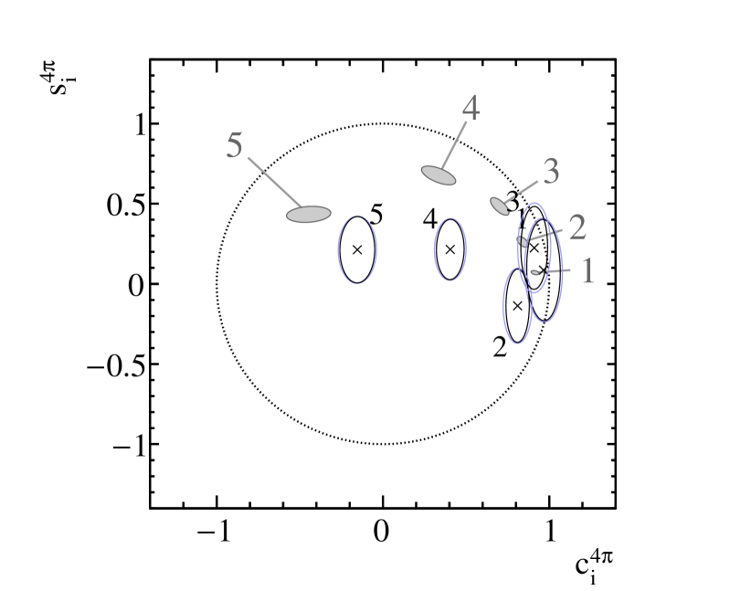
Alternative Binning

Optimal Binning

Optimal Alternative Binning

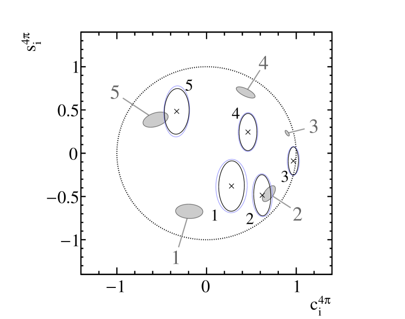
Figure 8: Each figure shows the hadronic parameters $c_{i}^{4\pi}$ and $s_{i}^{4\pi}$ measured using one of the $4\pi^{\pm}$ binning schemes discussed in Sec. 4 where $\mathcal{N}=5$. The grey shaded ellipses give the model predictions and uncertainties discussed in Sec. 4. The black (blue) ellipses show the measured values and statistical (statistical + systematic) uncertainties. In all cases the ellipse contains the $39.3\%$ confidence region, defined by the $\log\mathcal{L}_{\mathrm{max}}-\log\mathcal{L}=\frac{1}{2}$ contour, where $\log\mathcal{L}_{\mathrm{max}}$ is the maximum value of $\log\mathcal{L}$.

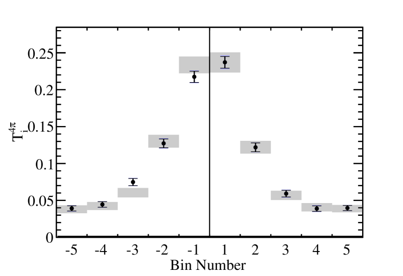
Variable $\Delta\delta^{4\pi}_{\mathbf{p}}$ binning

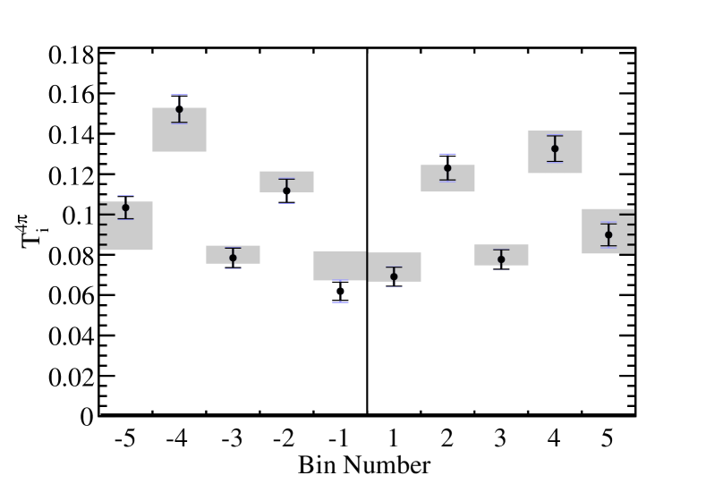
Alternative Binning

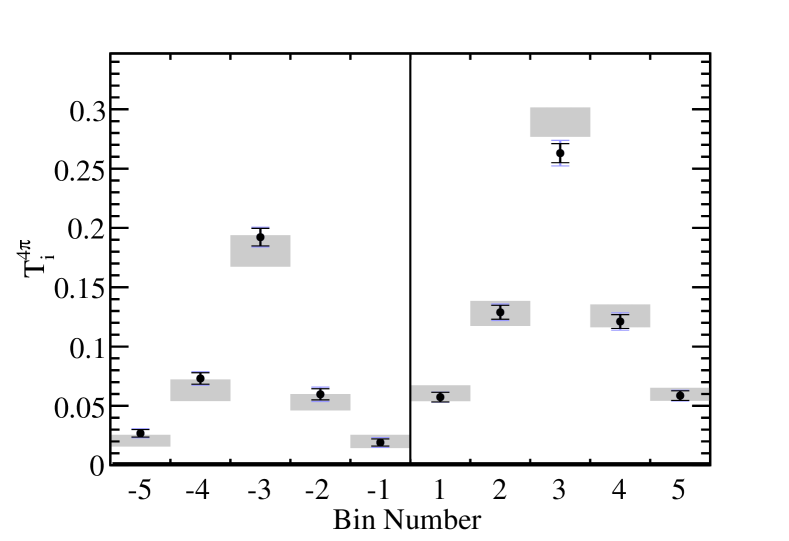
Optimal Binning

Optimal Alternative Binning

Figure 9: Each figure shows the hadronic parameters $T_{i}^{4\pi}$ and $\bar{T}_{i}^{4\pi}$ measured using one of the $4\pi^{\pm}$ binning schemes discussed in Sec. 4 where $\mathcal{N}=5$. The grey bands give the model predictions and uncertainties discussed in Sec. 4. The black (blue) points with errors give the measured values and statistical (statistical + systematic) uncertainties.

The measurement of the $4\pi^{\pm}$ hadronic parameters with statistical and systematic uncertainties is given in Tab. 7, with correlations in Appendix B. The results are compared to the model predictions in Fig. 8 and Fig. 9. The compatibility between the results and the model predictions is quantified by calculating the $\chi^{2}$ between to two, where all correlations are included. This is done independently for the $c_{i}^{4\pi}$/$s_{i}^{4\pi}$, and $T_{i}^{4\pi}$/$T_{i}^{4\pi}$ parameters, and for the combination, with the results in Tab. 6. The parameters $T_{i}^{4\pi}$ and $\bar{T}_{i}^{4\pi}$ show good agreement with the model predictions, which is expected since the model was determined from a fit to $D^{0}$ and $\kern 1.99997pt\overline{\kern-1.99997ptD}{}^{0}$ tagged data. The parameters $c_{i}^{f}$ and $s_{i}^{f}$ are in slight tension with the model predictions, with p-values ranging from $0.03$ to $0.18$, but they clearly follow the same general trend in the $c_{i}^{f}$-$s_{i}^{f}$ plane. It is worth repeating here that any incompatibility with the model will not introduce additional systematic uncertainties to a measurement of $\gamma$, but will only increase the statistical uncertainty.

Binning scheme	$c_{i}^{4\pi}$, $s_{i}^{4\pi}$		$T_{i}^{4\pi}$, $\bar{T}_{i}^{4\pi}$		$c_{i}^{4\pi}$, $s_{i}^{4\pi}$, $T_{i}^{4\pi}$, $\bar{T}_{i}^{4\pi}$
	$\chi^{2}$ / ndof	(p-value)	$\chi^{2}$ / ndof	(p-value)	$\chi^{2}$ / ndof	(p-value)
Equal $\Delta\delta^{4\pi}_{\mathbf{p}}$	19.9 / 10	( 0.03 )	7.4 / 9	( 0.59 )	30.0 / 19	( 0.05 )
Variable $\Delta\delta^{4\pi}_{\mathbf{p}}$	13.9 / 10	( 0.18 )	9.9 / 9	( 0.36 )	27.9 / 19	( 0.09 )
Alternate	16.6 / 10	( 0.08 )	10.3 / 9	( 0.33 )	27.0 / 19	( 0.10 )
Optimal	17.8 / 10	( 0.06 )	9.9 / 9	( 0.36 )	29.6 / 19	( 0.06 )
Optimal Alternate	13.7 / 10	( 0.19 )	17.2 / 9	( 0.05 )	31.2 / 19	( 0.04 )

Table 6: The compatibility of the measured $4\pi^{\pm}$ hadronic parameters with the model predictions for all binning schemes with $\mathcal{N}=5$.

Using the measured $4\pi^{\pm}$ hadronic parameters, the $C\!P$-even fraction of all phase space bins, $\tilde{{F}}^{4\pi}_{+}$, is calculated using the formula,

$$\tilde{{F}}^{4\pi}_{+}=\frac{1}{2}+{\frac{1}{2}\sum_{i}{c_{i}^{4\pi}\sqrt{T_{i}^{4\pi}\bar{T}_{i}^{4\pi}}}},$$ (8.1)

where the tilde indicates that a $\pi^{+}\pi^{-}$ mass window is excluded from the $D\!\rightarrow 4\pi^{\pm}$ phase space i.e. ${F}^{4\pi}_{+}$ represents the $C\!P$-even fraction for the entire phase space. The values of $\tilde{{F}}^{4\pi}_{+}$ are presented in Tab. 7, and are consistent among binning schemes. The nominal model is used to determine ${F}^{4\pi}_{+}-\tilde{{F}}^{4\pi}_{+}=-0.002\pm 0.002$ which can be used as a correction factor to determine ${F}^{4\pi}_{+}$ from the values of $\tilde{{F}}^{4\pi}_{+}$ in Tab. 7.

The $Q$ value of each binning scheme is determined using Eq. 4.8, and presented in Tab. 7; as expected, the optimal binning schemes give the largest $Q$ values. The $Q$ value for a single phase space bin is calculated, using $\tilde{{F}}^{4\pi}_{+}$, to be $0.505$. Therefore, based on the relative $Q$ values, and using the optimal-alternative binning scheme with $\mathcal{N}=5$, the increase in statistical power for a measurement of $\gamma$ is increased by $\sim 2.2$ times with respect to the phase space integrated case.

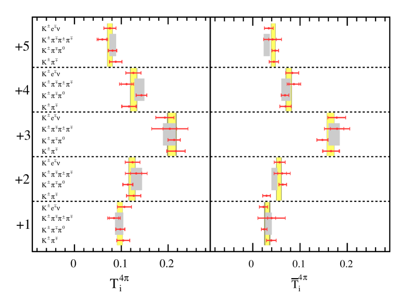
Figure 11: Constraints on the $T_{i}^{4\pi}$ and $\bar{T}_{i}^{4\pi}$ parameters (fraction of $D^{0}$ and $\kern 1.99997pt\overline{\kern-1.99997ptD}{}^{0}$ flavour tagged decays in each bin, repspectively) using the optimal alternative binning scheme with $\mathcal{N}=5$, determined using different subsets of tags. The grey bands show the model predictions and uncertainties. The red lines show the measured values and uncertainties when using a single subset of tags - the inner error bar shows the statistical uncertainty, and the outer error bar shows the combined statistical and systematic uncertainty. The yellow band shows the combined result using all subsets of tags - the lighter shade of yellow represents the statistical uncertainty, and the darker shade of yellow shows the combined statistical and systematic uncertainties.

The consistency of the $c_{i}^{4\pi}$ and $s_{i}^{4\pi}$ constraints obtained using different categories of final state is shown in Fig. 10 and Fig. 11 for the optimal alternative binning scheme with $\mathcal{N}=5$. For Fig. 10, each fit to one of the five categories ($C\!P\raisebox{0.3pt}{\scalebox{0.7}{+}}$, $C\!P\raisebox{0.1pt}{\scalebox{0.9}{-}}$, $\pi^{+}\pi^{-}\pi^{0}$, $K^{0}_{\rm\scriptscriptstyle S}\pi^{+}\pi^{-}$ and $K^{0}_{\rm\scriptscriptstyle L}\pi^{+}\pi^{-}$) uses all flavour and quasi-flavour tags. The constraints obtained are consistent between all categories of final state.

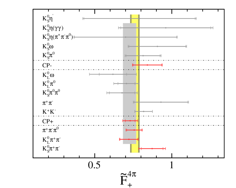
Figure 12: The $C\!P$-even fraction over all phase space bins, $\tilde{{F}}^{4\pi}_{+}$, determined using different subsets of tags. The grey bands show the model predictions and uncertainties. The red/grey lines show the measured values and uncertainties when using a single subset of tags - the inner error bar shows the statistical uncertainty, and the outer error bar shows the combined statistical and systematic uncertainty. The yellow band shows the combined result using all subsets of tags - the lighter shade of yellow represents the statistical uncertainty, and the darker shade of yellow shows the combined statistical and systematic uncertainties.

The fit is also run using a single $4\pi^{\pm}$ phase space bin, which gives $\tilde{{F}}^{4\pi}_{+}=0.760\pm 0.021\pm 0.021$. The consistency of this result is checked between all final states in Fig. 12, following a similar method to the one used to obtain Fig. 10. Good consistency is observed.

As a ‘default’ binning scheme, we take the optimal-alternative binning with $\mathcal{N}=5$, as this has highest predicted $Q$ value. The default binning scheme also has the largest measured $Q$ value, although this information was not used to pick the default binning since it could bias the results. The value of $\tilde{{F}}^{4\pi}_{+}$ determined using the default model is $0.771\pm 0.021\pm 0.010$, which leads to ${{F}}^{4\pi}_{+}=0.769\pm 0.021\pm 0.010\pm 0.002$, where the final uncertainty is due to the $K^{0}_{\rm\scriptscriptstyle S}$ veto. The value of ${{F}}^{4\pi}_{+}$ is an important input for determining the total $C\!P$ content of the neutral $D$ meson, which is related to the charm mixing parameter $y_{D}$ through Eq. 2.10 CPContOfDMeson .

Equal $\Delta\delta^{4\pi}_{\mathbf{p}}$ binning
i $c_{i}$ $s_{i}$ $T_{i}$ $\overline{T}_{i}$ 1 -0.881 $\pm$ 0.053 $\pm$ 0.044 -0.303 $\pm$ 0.149 $\pm$ 0.046 0.237 $\pm$ 0.008 $\pm$ 0.004 0.217 $\pm$ 0.008 $\pm$ 0.003 2 -0.501 $\pm$ 0.084 $\pm$ 0.046 -0.032 $\pm$ 0.201 $\pm$ 0.025 0.122 $\pm$ 0.006 $\pm$ 0.002 0.127 $\pm$ 0.006 $\pm$ 0.003 3 -0.450 $\pm$ 0.113 $\pm$ 0.064 -0.441 $\pm$ 0.228 $\pm$ 0.072 0.059 $\pm$ 0.004 $\pm$ 0.002 0.075 $\pm$ 0.005 $\pm$ 0.002 4 -0.201 $\pm$ 0.167 $\pm$ 0.068 -0.132 $\pm$ 0.304 $\pm$ 0.039 0.039 $\pm$ 0.004 $\pm$ 0.002 0.045 $\pm$ 0.004 $\pm$ 0.001 5 -0.397 $\pm$ 0.152 $\pm$ 0.036 -0.446 $\pm$ 0.381 $\pm$ 0.132 0.040 $\pm$ 0.004 $\pm$ 0.001 0.039 $\pm$ 0.004 $\pm$ 0.002 $\tilde{F}_{+}^{4\pi}$ -0.768 $\pm$ 0.021 $\pm$ 0.013 $Q$ -0.733 $\pm$ 0.052 $\pm$ 0.035 Variable $\Delta\delta^{4\pi}_{\mathbf{p}}$ binning
i $c_{i}$ $s_{i}$ $T_{i}$ $\overline{T}_{i}$ 1 -0.966 $\pm$ 0.101 $\pm$ 0.052 -0.086 $\pm$ 0.316 $\pm$ 0.068 0.069 $\pm$ 0.005 $\pm$ 0.001 0.062 $\pm$ 0.004 $\pm$ 0.003 2 -0.810 $\pm$ 0.070 $\pm$ 0.051 -0.136 $\pm$ 0.229 $\pm$ 0.051 0.123 $\pm$ 0.006 $\pm$ 0.003 0.112 $\pm$ 0.006 $\pm$ 0.002 3 -0.910 $\pm$ 0.080 $\pm$ 0.059 -0.225 $\pm$ 0.259 $\pm$ 0.107 0.078 $\pm$ 0.005 $\pm$ 0.001 0.078 $\pm$ 0.005 $\pm$ 0.002 4 -0.405 $\pm$ 0.083 $\pm$ 0.046 -0.215 $\pm$ 0.188 $\pm$ 0.041 0.133 $\pm$ 0.006 $\pm$ 0.003 0.152 $\pm$ 0.006 $\pm$ 0.003 5 -0.154 $\pm$ 0.105 $\pm$ 0.047 -0.213 $\pm$ 0.207 $\pm$ 0.031 0.090 $\pm$ 0.005 $\pm$ 0.003 0.103 $\pm$ 0.006 $\pm$ 0.002 $\tilde{F}_{+}^{4\pi}$ -0.772 $\pm$ 0.021 $\pm$ 0.010 $Q$ -0.698 $\pm$ 0.049 $\pm$ 0.020 Alternative binning
i $c_{i}$ $s_{i}$ $T_{i}$ $\overline{T}_{i}$ 1 -0.205 $\pm$ 0.189 $\pm$ 0.094 -0.057 $\pm$ 0.384 $\pm$ 0.127 0.057 $\pm$ 0.004 $\pm$ 0.001 0.019 $\pm$ 0.003 $\pm$ 0.003 2 -0.445 $\pm$ 0.105 $\pm$ 0.066 -0.041 $\pm$ 0.259 $\pm$ 0.073 0.129 $\pm$ 0.006 $\pm$ 0.004 0.060 $\pm$ 0.005 $\pm$ 0.004 3 -0.888 $\pm$ 0.053 $\pm$ 0.045 -0.150 $\pm$ 0.159 $\pm$ 0.027 0.263 $\pm$ 0.008 $\pm$ 0.007 0.192 $\pm$ 0.007 $\pm$ 0.004 4 -0.530 $\pm$ 0.097 $\pm$ 0.044 -0.239 $\pm$ 0.209 $\pm$ 0.084 0.121 $\pm$ 0.006 $\pm$ 0.004 0.073 $\pm$ 0.005 $\pm$ 0.003 5 -0.451 $\pm$ 0.162 $\pm$ 0.053 -0.238 $\pm$ 0.416 $\pm$ 0.157 0.059 $\pm$ 0.004 $\pm$ 0.002 0.027 $\pm$ 0.003 $\pm$ 0.002 $\tilde{F}_{+}^{4\pi}$ -0.764 $\pm$ 0.022 $\pm$ 0.011 $Q$ -0.702 $\pm$ 0.051 $\pm$ 0.027 Optimal binning
i $c_{i}$ $s_{i}$ $T_{i}$ $\overline{T}_{i}$ 1 -0.949 $\pm$ 0.057 $\pm$ 0.039 -0.041 $\pm$ 0.171 $\pm$ 0.041 0.193 $\pm$ 0.007 $\pm$ 0.004 0.173 $\pm$ 0.007 $\pm$ 0.003 2 -0.641 $\pm$ 0.110 $\pm$ 0.073 -0.331 $\pm$ 0.257 $\pm$ 0.087 0.045 $\pm$ 0.004 $\pm$ 0.004 0.123 $\pm$ 0.006 $\pm$ 0.005 3 -0.542 $\pm$ 0.094 $\pm$ 0.059 -0.034 $\pm$ 0.224 $\pm$ 0.063 0.135 $\pm$ 0.006 $\pm$ 0.005 0.070 $\pm$ 0.005 $\pm$ 0.004 4 -0.309 $\pm$ 0.123 $\pm$ 0.073 -0.294 $\pm$ 0.236 $\pm$ 0.058 0.054 $\pm$ 0.005 $\pm$ 0.003 0.092 $\pm$ 0.005 $\pm$ 0.002 5 -0.492 $\pm$ 0.130 $\pm$ 0.041 -0.665 $\pm$ 0.256 $\pm$ 0.100 0.069 $\pm$ 0.004 $\pm$ 0.002 0.045 $\pm$ 0.004 $\pm$ 0.002 $\tilde{F}_{+}^{4\pi}$ -0.768 $\pm$ 0.021 $\pm$ 0.012 $Q$ -0.757 $\pm$ 0.052 $\pm$ 0.026 Optimal-alternative binning
i $c_{i}$ $s_{i}$ $T_{i}$ $\overline{T}_{i}$ 1 -0.279 $\pm$ 0.143 $\pm$ 0.101 -0.379 $\pm$ 0.291 $\pm$ 0.104 0.096 $\pm$ 0.005 $\pm$ 0.002 0.032 $\pm$ 0.004 $\pm$ 0.005 2 -0.622 $\pm$ 0.095 $\pm$ 0.059 -0.486 $\pm$ 0.237 $\pm$ 0.072 0.123 $\pm$ 0.006 $\pm$ 0.004 0.055 $\pm$ 0.004 $\pm$ 0.003 3 -0.969 $\pm$ 0.057 $\pm$ 0.038 -0.089 $\pm$ 0.162 $\pm$ 0.038 0.202 $\pm$ 0.007 $\pm$ 0.005 0.164 $\pm$ 0.007 $\pm$ 0.003 4 -0.463 $\pm$ 0.099 $\pm$ 0.046 -0.245 $\pm$ 0.215 $\pm$ 0.067 0.134 $\pm$ 0.006 $\pm$ 0.005 0.077 $\pm$ 0.005 $\pm$ 0.004 5 -0.332 $\pm$ 0.138 $\pm$ 0.041 -0.484 $\pm$ 0.263 $\pm$ 0.132 0.074 $\pm$ 0.005 $\pm$ 0.002 0.043 $\pm$ 0.004 $\pm$ 0.003 $\tilde{F}_{+}^{4\pi}$ -0.771 $\pm$ 0.021 $\pm$ 0.010 $Q$ -0.760 $\pm$ 0.057 $\pm$ 0.017

Table 7: The hadronic parameters measured for each of the $4\pi^{\pm}$ binning schemes discussed in Sec. 4 where $\mathcal{N}=5$. The first uncertainty given is statistical, and the second systematic. Also given is the CP-even fraction, $\tilde{{F}}^{4\pi}_{+}$, and the $Q$ value, defined in Sec. 4; the uncertainties on these parameters are propagated from the statistical and systematic uncertainties on the hadronic parameters.

Equal $\Delta\delta^{4\pi}_{\mathbf{p}}$ binning

Variable $\Delta\delta^{4\pi}_{\mathbf{p}}$ binning

Equal $\Delta\delta^{4\pi}_{\mathbf{p}}$ binning

Figure 10: Constraints on the $c_{i}^{4\pi}$ and $s_{i}^{4\pi}$ parameters using the optimal alternative binning scheme with $\mathcal{N}=5$, determined using different subsets of tags. The grey bands show the model predictions and uncertainties. The red lines show the measured values and uncertainties when using a single subset of tags - the inner error bar shows the statistical uncertainty, and the outer error bar shows the combined statistical and systematic uncertainty. The yellow band shows the combined result using all subsets of tags - the lighter shade of yellow represents the statistical uncertainty, and the darker shade of yellow shows the combined statistical and systematic uncertainties.

9 Sensitivity studies

In this section the measured $4\pi^{\pm}$ hadronic parameters from Sec. 8 are used to simulate $B^{\pm}\!\rightarrow DK^{\pm},D\!\rightarrow 4\pi^{\pm}$ datasets, which in turn are used to estimate the sensitivity to $\gamma$. Three scenarios with different event yields are studied, based on measured and extrapolated $B^{\pm}\!\rightarrow DK^{\pm},D\!\rightarrow 4\pi^{\pm}$ event yields from LHCb: “LHCb run I”, with event yields of $\sim 1,500$ already recorded by LHCb with $3\mbox{\,fb}^{-1}$ cpObsTwoAndFourBody of data; “LHCb run II”, with plausible event yields of $\sim 6,500$ at the end of the next LHC data taking period with approximately twice the collision energy and an estimated $8\mbox{\,fb}^{-1}$ of data; and “LHCb phase 1 upgrade”, with plausible event yields of $\sim 100,000$ after phase 1 of the LHCb upgrade. The increase in the heavy flavour cross section at higher collision energies is accounted for, along with the expected improvement in trigger efficiency at the LHCb phase 1 upgrade LHCbUpgradeCDR . The extrapolations have of course large uncertainties. The presence of background and systematic effects has been neglected in these studies, which is a reasonable assumption given previous measurements cpObsTwoAndFourBody .

Toy datasets of $B^{\pm}\!\rightarrow DK^{\pm},D\!\rightarrow 4\pi^{\pm}$ decays are generated using Eq. 2.13 and Eq. 2.14 with $\delta_{B}=140^{\circ}$, $\gamma=70^{\circ}$ and $r_{B}=0.1$. For each toy dataset, the central values of the $4\pi^{\pm}$ hadronic parameters are randomly sampled from the measured values and uncertainties. When fitting the toy datasets, the parameters $\delta_{B}$, $\gamma$, $r_{B}$ and an overall normalisation parameter are allowed to float, whereas the $4\pi^{\pm}$ hadronic parameters are fixed to their measured values. Therefore, the uncertainties obtained from the fit only account for the finite $B^{\pm}\!\rightarrow DK^{\pm},D\!\rightarrow 4\pi^{\pm}$ statistics, $\sigma_{\mathrm{stat}}$. The uncertainties on the parameters $c_{i}^{4\pi}$ and $s_{i}^{4\pi}$ are propagated to $\delta_{B}$, $\gamma$ and $r_{B}$ by repeating the fit 200 times, where for each fit $c_{i}^{4\pi}$ and $s_{i}^{4\pi}$ are randomly sampled from their associated covariance matrix. The covariance of the values obtained is used to assign an uncertainty, $\sigma_{\mathrm{had}}$. The parameters $K_{i}^{4\pi}$ and $\bar{K}_{i}^{4\pi}$ can be determined to an arbitrarily high precision at LHCb using $D^{*+}\!\rightarrow D^{0}\pi^{+}$ decays, so the uncertainties on these parameters are neglected. As an alternative approach, the $c_{i}^{4\pi}$ and $s_{i}^{4\pi}$ parameters are Gaussian constrained in the fit, but this method was found to give a heavily biased estimate of $\gamma$, up to $70\%$ of the statistical uncertainty. The nominal fit method gives good coverage and small biases of less than $10\%$.

The expected $\gamma$ uncertainties are presented in Tab. 8 for several binning schemes. For each case the expected $\gamma$ uncertainty is median uncertainty determined from fits to 100 simulated datasets. For each binning scheme type the uncertainty on $\gamma$ generally decreases with increasing numbers of bins - for illustration, the uncertainty on $\gamma$ is shown for the optimal-alternative binning scheme for $\mathcal{N}=2-5$ in Tab. 8. The $\gamma$ uncertainties are also compared between different binning scheme types with $\mathcal{N}=5$; all result in similar values of $\sigma_{\mathrm{stat}}(\gamma)$, although the values of $\sigma_{\mathrm{had}}(\gamma)$ are notably larger for the ‘variable $\Delta\delta^{4\pi}_{\mathbf{p}}$’ and the ‘alternative’ binning schemes. This is likely due to the measured central values of the $s_{i}^{4\pi}$ parameters being consistent with zero for these schemes. For the default binning (optimal alternative with $\mathcal{N}=5$) the expected uncertainties are $(18\oplus 13)^{\circ}$, $(10\oplus 7)^{\circ}$ and $(2.5\oplus 4.4)^{\circ}$ for the LHCb “Run I”, “Run II” and “Phase 1 Upgrade” scenarios, respectively, where the uncertainties are given in the form $\sigma_{\mathrm{stat}}\left(\gamma\right)\oplus\sigma_{\mathrm{had}}\left(\gamma\right)$.

Since $\sigma_{\mathrm{had}}\left(\gamma\right)\approx\sigma_{\mathrm{stat}}\left(\gamma\right)$ for the LHCb “Run I” and “Run II” scenarios, and $\sigma_{\mathrm{had}}\left(\gamma\right)>\sigma_{\mathrm{stat}}\left(\gamma\right)$ for the “Phase 1 Upgrade” scenario, it is interesting to consider the impact that BESIII could have on reducing $\sigma_{\mathrm{had}}\left(\gamma\right)$. Currently BESIII have collected 2.9$\mbox{\,fb}^{-1}$ of $e^{+}e^{-}$ collisions at the $\psi(3770)$ resonance, and a further $\sim 7\mbox{\,fb}^{-1}$ is planned for the future. These datasets correspond to approximately 3.5 and 12 times the amount collected by CLEO-c, respectively. It is assumed that the uncertainties on the $4\pi^{\pm}$ hadronic parameters would be reduced by $1/\sqrt{3.5}$ and $1/\sqrt{12}$, respectively, compared to the constraints obtained in Sec. 8. The central values of the estimated BESIII measurements are different for each simulated dataset, and are randomly sampled from the constraints obtained in Sec. 8. Fig. 13 shows, for the default binning scheme, the expected values of $\sigma_{\mathrm{had}}\left(\gamma\right)$ for different numbers of $B^{\pm}\!\rightarrow DK^{\pm},D\!\rightarrow 4\pi^{\pm}$ decays. This is shown for the hadronic parameter constraints measured in this paper, and the expected constraints for the two BESIII data taking periods. With $10.0\mbox{\,fb}^{-1}$ of BESIII data, the expected $\gamma$ uncertainties become $(18\oplus 3)^{\circ}$, $(10\oplus 1.7)^{\circ}$ and $(2.5\oplus 1.2)^{\circ}$ for the LHCb “Run I”, “Run II” and “Phase 1 Upgrade” scenarios, respectively. It is also possible that BESIII could make further gains in sensitivity by using additional numbers of phase space bins. Improved constraints on the $4\pi^{\pm}$ hadronic parameters could be obtained using $D$-mixing, as has been done for the $K^{\pm}\pi^{\mp}\pi^{\pm}\pi^{\mp}$ final state in Ref. K3piLHCb ; this would require further investigation.

		$\left(\sigma_{\mathrm{stat}}\left(\gamma\right)\oplus\sigma_{\mathrm{had}}\left(\gamma\right)\right)~{}[^{\circ}]$
		LHCb	LHCb	LHCb
Binning scheme	$\mathcal{N}$	Run I	Run II	Ph.1 Upgrade
Optimal Alternative	2	20.4 $\oplus$ 27.0	16.2 $\oplus$ 20.5	04.6 $\oplus$ 15.6
	3	18.0 $\oplus$ 10.1	010.0 $\oplus$ 05.4	02.6 $\oplus$ 03.6
	4	18.2 $\oplus$ 15.9	10.5 $\oplus$ 10.6	02.9 $\oplus$ 06.5
(default binning)	5	18.0 $\oplus$ 13.2	09.7 $\oplus$ 07.4	02.5 $\oplus$ 04.4
Equal $\Delta\delta^{4\pi}_{\mathbf{p}}$	5	16.7 $\oplus$ 12.6	09.2 $\oplus$ 07.2	02.4 $\oplus$ 04.0
Variable $\Delta\delta^{4\pi}_{\mathbf{p}}$	5	19.8 $\oplus$ 23.3	10.2 $\oplus$ 14.7	02.9 $\oplus$ 11.1
Alternative	5	19.2 $\oplus$ 24.6	11.4 $\oplus$ 18.1	03.3 $\oplus$ 14.2
Optimal	5	17.3 $\oplus$ 13.9	010.0 $\oplus$ 07.9	02.6 $\oplus$ 05.0

Table 8: Expected $\gamma$ sensitivity determined from simulated samples of $B^{\pm}\!\rightarrow DK^{\pm},D\!\rightarrow 4\pi^{\pm}$ decays for a variety of $D\!\rightarrow 4\pi^{\pm}$ binning schemes. Details of the simulation and fitting procedure can be found in the text. The uncertainties are given for three different data taking periods of the LHCb experiment, where the number of signal decays in each case it taken/extrapolated from existing measurements. The uncertainty on $\gamma$ comes from two sources: the uncertainty due to to limited $B^{\pm}\!\rightarrow DK^{\pm},D\!\rightarrow 4\pi^{\pm}$ statistics, $\sigma_{\mathrm{stat}}\left(\gamma\right)$; and the uncertainty due to limited knowledge of the $4\pi^{\pm}$ hadronic parameters that are measured in this paper, $\sigma_{\mathrm{had}}\left(\gamma\right)$. Both uncertainties are shown in the table, and are given in the format $\left(\sigma_{\mathrm{stat}}\left(\gamma\right)\oplus\sigma_{\mathrm{had}}\left(\gamma\right)\right)$. All expected uncertainties are the median uncertainty from 100 simulated experiments.

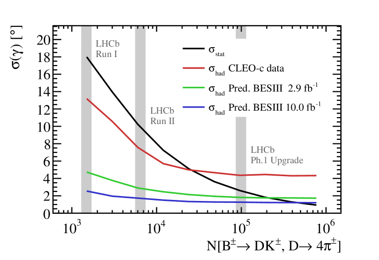
Figure 13: Expected $\gamma$ uncertainties obtained using different numbers of $B^{\pm}\!\rightarrow DK^{\pm},D\!\rightarrow 4\pi^{\pm}$ decays and the default binning scheme. The black line shows the estimated uncertainty due to limited $B^{\pm}\!\rightarrow DK^{\pm},D\!\rightarrow 4\pi^{\pm}$ statistics. The red, green and blue lines shows the estimated uncertainty due to the measured/predicted constraints on the $4\pi^{\pm}$ hadronic parameters from CLEO-c data with 0.818$\mbox{\,fb}^{-1}$, BES III with 2.9$\mbox{\,fb}^{-1}$, and BES III with 10.0$\mbox{\,fb}^{-1}$, respectively. The grey bands highlight the event numbers that correspond to different LHCb data taking periods.

10 Summary

Using 818 $\rm pb^{-1}$ of $e^{+}e^{-}$ collision data collected by the CLEO-c detector, the hadronic parameters of the $D\!\rightarrow 4\pi^{\pm}$ decay are measured in bins of phase space for the first time. This allows the UT angle $\gamma$ to be determined using only $B^{\pm}\!\rightarrow DK^{\pm}$ decays where $D$ decays to the $4\pi^{\pm}$ final state; previously only phase space integrated measurements have been possible FPlusFourPi ; cpObsTwoAndFourBody , which need to be combined with other final states to obtain constraints on $\gamma$ cpObsTwoAndFourBody ; LHCbGamCom .

The phase space of the $D\!\rightarrow 4\pi^{\pm}$ decay is divided into bins based on the nominal amplitude model from Ref. fourpimodel . The equal and variable $\Delta\delta^{4\pi}_{\mathbf{p}}$ binning schemes are based on an equal/variable division of $\Delta\delta^{4\pi}_{\mathbf{p}}$, whereas the alternate binning scheme also uses the relative magnitude of $D^{0}\!\rightarrow 4\pi^{\pm}$ to $\kern 1.99997pt\overline{\kern-1.99997ptD}{}^{0}\!\rightarrow 4\pi^{\pm}$ amplitudes. The optimal and optimal alternative binning schemes are defined to optimise the expected sensitivity to $\gamma$ in $B^{\pm}\!\rightarrow DK^{\pm}$ decays. Although an amplitude model is used to inspire the binning schemes, the results are model-unbiased; any modelling deficiencies will only result in an increased statistical uncertainty on $\gamma$.

Since amplitude models can be notoriously difficult to reproduce, it is useful to have a model-implementation independent method to represent a binning scheme. The phase space of the $D\!\rightarrow 4\pi^{\pm}$ decay is five-dimensional, so using traditional techniques to divide the phase space into $N^{5}$ equally sized hypervolumes, where each is assigned a bin-number, would result in an unmanageable number of hypervolumes. An adaptive binning scheme is developed that uses an array of differently sized hypervolumes to drastically reduce the total number of hypervolumes needed, typically around $250,000$.

The measured values of the hadronic parameters are compared to the model-predictions, which show good agreement for the parameters $T_{i}^{4\pi}$ and $\bar{T}_{i}^{4\pi}$, but a slight tension for $c_{i}^{4\pi}$ and $s_{i}^{4\pi}$. This could either be due to statistical fluctuations, which could be tested with larger datasets at BESIII, or a possible residual mismodelling of the phase motion across the $D\!\rightarrow 4\pi^{\pm}$ phase space in Ref. fourpimodel .

The consistency of the results is checked using different subsets of final states, which give statistically compatible results. The $C\!P$ even fraction over all phase space bins, $\tilde{F}_{+}^{4\pi}$, is observed to be consistent between all binning schemes. Using the ‘default’ binning scheme, ${F}_{+}^{4\pi}$ is determined as $0.769\pm 0.021\pm 0.010\pm 0.002$ where the uncertainties are statistical, systematic, and from the $K^{0}_{\rm\scriptscriptstyle S}$ veto, respectively. This is the most precise determination ${F}_{+}^{4\pi}$ to date.

Using the $4\pi^{\pm}$ hadronic parameters measured in this paper, samples of $B^{\pm}\!\rightarrow DK^{\pm},D\rightarrow 4\pi^{\pm}$ decays are simulated, then used to estimate the potential sensitivity to $\gamma$. It is shown that, using estimated sample sizes from LHCb at the end of its current running period (“Run II”) and the hadronic parameter constraints from this paper, constraints of $\sigma(\gamma)=(10\oplus 7)^{\circ}$ could be obtained, potentially making $4\pi^{\pm}$ one of the most sensitive final states for a measurement of $\gamma$. The first uncertainty is due to limited $B^{\pm}\!\rightarrow DK^{\pm}$ statistics, and the second is due to uncertainties on the $4\pi^{\pm}$ hadronic parameters. It is shown that the latter uncertainty could be reduced to around $1.7^{\circ}$ by using current and future BESIII datasets.

11 Acknowledgements

This analysis was performed using CLEO-c data. The authors, some of whom were members of CLEO, are grateful to the collaboration for the privilege of using these data. We also thank Guy Wilkinson, Sneha Malde, Jim Libby, Tim Gershon, Philippe D’Argent, Kostas Petridis and Vincenzo Vagnoni for their valuable feedback on the paper draft. We also acknowledge the support of the UK Science and Technology Facilities Council (STFC), and the European Research Council’s support under Framework 7 / ERC Grant Agreement number 307737.

Appendix A Helicity variables

In this paper the variables $\{m_{+},m_{-},\cos\theta_{+},\cos\theta_{-},\phi\}$ are used to parameterise a point in the $D\!\rightarrow 4\pi^{\pm}$ phase space; their full definition is given in this appendix. The variables $m_{+}$ and $m_{-}$ are defined,

$$m_{+}^{2}=(p_{\pi^{+}_{1}}+p_{\pi^{+}_{2}})^{2},$$ (A.1)

$$m_{-}^{2}=(p_{\pi^{-}_{1}}+p_{\pi^{-}_{2}})^{2},$$ (A.2)

where $p_{\pi^{+}_{1}}$ and $p_{\pi^{+}_{2}}$ ($p_{\pi^{-}_{1}}$ and $p_{\pi^{-}_{2}}$) are the four-vectors of the positively (negatively) charged pions in the final state. The cosine of the two helicity angles, $\cos\theta_{+}$ and $\cos\theta_{-}$, are defined,

$$\cos\theta_{+}=\frac{\vec{p}_{\pi^{+}_{1}}\cdot\vec{p}_{D}}{|\vec{p}_{\pi^{+}_{1}}||\vec{p}_{D}|}\mathrm{\ \ \ evaluated\ in\ the\ frame\ where\ \ \ }\vec{p}_{\pi^{+}_{1}}+\vec{p}_{\pi^{+}_{2}}=0$$ (A.3)

$$\cos\theta_{-}=\frac{\vec{p}_{\pi^{-}_{1}}\cdot\vec{p}_{D}}{|\vec{p}_{\pi^{-}_{1}}||\vec{p}_{D}|}\mathrm{\ \ \ evaluated\ in\ the\ frame\ where\ \ \ }\vec{p}_{\pi^{-}_{1}}+\vec{p}_{\pi^{-}_{2}}=0$$ (A.4)

where $\vec{p}_{\pi^{\pm}_{1,2}}$ is the three-vector associated to ${p}_{\pi^{\pm}_{1,2}}$. The angle between the $\pi^{+}\pi^{+}$ and $\pi^{-}\pi^{-}$ decay planes, $\phi$, is defined by,

$$\sin\phi =\left[\frac{(\vec{p}_{\pi^{+}_{1}}\times\vec{p}_{\pi^{+}_{2}})}{|\vec{p}_{\pi^{+}_{1}}\times\vec{p}_{\pi^{+}_{2}}|}\times\frac{(\vec{p}_{\pi^{-}_{1}}\times\vec{p}_{\pi^{-}_{2}})}{|\vec{p}_{\pi^{-}_{1}}\times\vec{p}_{\pi^{-}_{2}}|}\right]\cdot\frac{\vec{p}_{\pi^{-}_{1}}+\vec{p}_{\pi^{-}_{2}}}{|\vec{p}_{\pi^{-}_{1}}+\vec{p}_{\pi^{-}_{2}}|}\mathrm{\ \ \ evaluated\ in\ the\ }\vec{p}_{D}=0\mathrm{\ frame}$$ (A.5)

$$\cos\phi =\left[\frac{(\vec{p}_{\pi^{+}_{1}}\times\vec{p}_{\pi^{+}_{2}})}{|\vec{p}_{\pi^{+}_{1}}\times\vec{p}_{\pi^{+}_{2}}|}\ \cdot\ \frac{(\vec{p}_{\pi^{-}_{1}}\times\vec{p}_{\pi^{-}_{2}})}{|\vec{p}_{\pi^{-}_{1}}\times\vec{p}_{\pi^{-}_{2}}|}\right]\hskip 65.44142pt\mathrm{\ \ \ evaluated\ in\ the\ }\vec{p}_{D}=0\mathrm{\ frame}$$ (A.6)

Note that there is a conventional choice that can cause $\phi\rightarrow-\phi$, so it is important to copy these expressions exactly.

Appendix B Statistical and systematic correlations

Equal $\Delta\delta^{4\pi}_{\mathbf{p}}$ binning statistical correlations
$c^{4\pi}_{+1}$ $c^{4\pi}_{+2}$ $c^{4\pi}_{+3}$ $c^{4\pi}_{+4}$ $c^{4\pi}_{+5}$ $s^{4\pi}_{+1}$ $s^{4\pi}_{+2}$ $s^{4\pi}_{+3}$ $s^{4\pi}_{+4}$ $s^{4\pi}_{+5}$ $T^{4\pi}_{+1}$ $T^{4\pi}_{+2}$ $T^{4\pi}_{+3}$ $T^{4\pi}_{+4}$ $T^{4\pi}_{+5}$ $T^{4\pi}_{-1}$ $T^{4\pi}_{-2}$ $T^{4\pi}_{-3}$ $T^{4\pi}_{-4}$ $T^{4\pi}_{-5}$ $c^{4\pi}_{+1}$ 1.00 0.03 0.02 0.00 0.01 0.01 0.00 0.01 0.00 0.00 -0.04 0.03 0.02 0.02 0.02 -0.08 0.04 0.03 0.02 0.02 $c^{4\pi}_{+2}$ 0.03 1.00 0.02 0.02 0.02 -0.00 0.03 0.00 0.00 -0.01 0.03 -0.06 0.01 0.00 0.00 0.03 -0.05 0.01 0.01 0.00 $c^{4\pi}_{+3}$ 0.02 0.02 1.00 0.02 0.01 0.00 0.00 0.00 -0.00 0.00 0.02 0.01 -0.08 0.00 0.00 0.02 0.01 -0.03 0.00 0.00 $c^{4\pi}_{+4}$ 0.00 0.02 0.02 1.00 0.02 -0.01 0.00 -0.01 0.03 -0.01 0.02 0.01 0.01 -0.06 0.00 0.02 0.01 0.01 -0.06 0.00 $c^{4\pi}_{+5}$ 0.01 0.02 0.01 0.02 1.00 -0.01 -0.00 -0.01 -0.00 -0.09 0.01 0.00 0.00 -0.00 -0.03 0.01 0.00 0.00 -0.00 -0.03 $s^{4\pi}_{+1}$ 0.01 -0.00 0.00 -0.01 -0.01 1.00 -0.01 0.05 0.01 0.02 -0.02 0.00 -0.01 0.00 0.01 0.00 0.00 0.01 0.00 0.00 $s^{4\pi}_{+2}$ 0.00 0.03 0.00 0.00 -0.00 -0.01 1.00 -0.00 0.02 0.00 -0.00 0.00 -0.00 -0.00 0.00 0.00 -0.01 0.00 0.00 -0.00 $s^{4\pi}_{+3}$ 0.01 0.00 0.00 -0.01 -0.01 0.05 -0.00 1.00 -0.00 0.01 0.00 0.00 -0.06 0.00 0.00 0.00 0.00 0.04 0.00 0.00 $s^{4\pi}_{+4}$ 0.00 0.00 -0.00 0.03 -0.00 0.01 0.02 -0.00 1.00 -0.01 -0.00 0.00 -0.00 0.01 0.00 0.01 0.00 0.00 -0.03 -0.00 $s^{4\pi}_{+5}$ 0.00 -0.01 0.00 -0.01 -0.09 0.02 0.00 0.01 -0.01 1.00 -0.00 -0.00 -0.00 0.00 -0.03 -0.00 -0.00 0.00 0.00 0.05 $T^{4\pi}_{+1}$ -0.04 0.03 0.02 0.02 0.01 -0.02 -0.00 0.00 -0.00 -0.00 1.00 -0.17 -0.11 -0.10 -0.10 -0.42 -0.17 -0.14 -0.11 -0.10 $T^{4\pi}_{+2}$ 0.03 -0.06 0.01 0.01 0.00 0.00 0.00 0.00 0.00 -0.00 -0.17 1.00 -0.08 -0.07 -0.07 -0.16 -0.27 -0.09 -0.07 -0.07 $T^{4\pi}_{+3}$ 0.02 0.01 -0.08 0.01 0.00 -0.01 -0.00 -0.06 -0.00 -0.00 -0.11 -0.08 1.00 -0.05 -0.05 -0.11 -0.08 -0.23 -0.05 -0.04 $T^{4\pi}_{+4}$ 0.02 0.00 0.00 -0.06 -0.00 0.00 -0.00 0.00 0.01 0.00 -0.10 -0.07 -0.05 1.00 -0.04 -0.10 -0.07 -0.05 -0.16 -0.04 $T^{4\pi}_{+5}$ 0.02 0.00 0.00 0.00 -0.03 0.01 0.00 0.00 0.00 -0.03 -0.10 -0.07 -0.05 -0.04 1.00 -0.09 -0.07 -0.05 -0.04 -0.15 $T^{4\pi}_{-1}$ -0.08 0.03 0.02 0.02 0.01 0.00 0.00 0.00 0.01 -0.00 -0.42 -0.16 -0.11 -0.10 -0.09 1.00 -0.16 -0.11 -0.10 -0.09 $T^{4\pi}_{-2}$ 0.04 -0.05 0.01 0.01 0.00 0.00 -0.01 0.00 0.00 -0.00 -0.17 -0.27 -0.08 -0.07 -0.07 -0.16 1.00 -0.09 -0.07 -0.07 $T^{4\pi}_{-3}$ 0.03 0.01 -0.03 0.01 0.00 0.01 0.00 0.04 0.00 0.00 -0.14 -0.09 -0.23 -0.05 -0.05 -0.11 -0.09 1.00 -0.05 -0.05 $T^{4\pi}_{-4}$ 0.02 0.01 0.00 -0.06 -0.00 0.00 0.00 0.00 -0.03 0.00 -0.11 -0.07 -0.05 -0.16 -0.04 -0.10 -0.07 -0.05 1.00 -0.04 $T^{4\pi}_{-5}$ 0.02 0.00 0.00 0.00 -0.03 0.00 -0.00 0.00 -0.00 0.05 -0.10 -0.07 -0.04 -0.04 -0.15 -0.09 -0.07 -0.05 -0.04 1.00

Equal $\Delta\delta^{4\pi}_{\mathbf{p}}$ binning systematic correlations
$c^{4\pi}_{+1}$ $c^{4\pi}_{+2}$ $c^{4\pi}_{+3}$ $c^{4\pi}_{+4}$ $c^{4\pi}_{+5}$ $s^{4\pi}_{+1}$ $s^{4\pi}_{+2}$ $s^{4\pi}_{+3}$ $s^{4\pi}_{+4}$ $s^{4\pi}_{+5}$ $T^{4\pi}_{+1}$ $T^{4\pi}_{+2}$ $T^{4\pi}_{+3}$ $T^{4\pi}_{+4}$ $T^{4\pi}_{+5}$ $T^{4\pi}_{-1}$ $T^{4\pi}_{-2}$ $T^{4\pi}_{-3}$ $T^{4\pi}_{-4}$ $T^{4\pi}_{-5}$ $c^{4\pi}_{+1}$ 1.00 -0.01 0.00 0.01 -0.01 -0.00 -0.04 -0.00 -0.01 0.01 0.01 -0.01 0.00 0.01 -0.00 -0.02 0.00 0.00 -0.02 0.03 $c^{4\pi}_{+2}$ -0.01 1.00 0.04 0.04 0.05 0.01 0.06 0.01 0.04 0.00 -0.00 0.06 0.00 -0.02 -0.07 -0.00 -0.04 0.05 0.03 -0.01 $c^{4\pi}_{+3}$ 0.00 0.04 1.00 0.04 0.04 0.03 -0.01 0.00 -0.00 -0.01 -0.00 0.04 -0.00 0.01 -0.01 -0.00 -0.05 0.06 -0.00 -0.01 $c^{4\pi}_{+4}$ 0.01 0.04 0.04 1.00 0.05 0.02 0.05 0.01 -0.00 0.01 0.02 -0.03 -0.01 -0.01 0.02 0.00 -0.03 0.04 0.00 -0.00 $c^{4\pi}_{+5}$ -0.01 0.05 0.04 0.05 1.00 0.07 -0.03 0.00 -0.00 -0.02 0.03 -0.02 -0.02 -0.02 0.02 0.03 -0.05 0.00 -0.00 -0.01 $s^{4\pi}_{+1}$ -0.00 0.01 0.03 0.02 0.07 1.00 0.08 -0.01 -0.02 -0.01 -0.10 0.09 0.00 -0.02 0.09 0.12 -0.06 0.02 -0.00 -0.02 $s^{4\pi}_{+2}$ -0.04 0.06 -0.01 0.05 -0.03 0.08 1.00 0.04 0.03 -0.03 -0.11 -0.13 -0.01 -0.01 0.12 0.19 0.09 0.01 0.04 -0.20 $s^{4\pi}_{+3}$ -0.00 0.01 0.00 0.01 0.00 -0.01 0.04 1.00 0.00 -0.01 0.00 -0.05 -0.01 -0.01 0.02 0.01 0.02 -0.00 0.04 -0.02 $s^{4\pi}_{+4}$ -0.01 0.04 -0.00 -0.00 -0.00 -0.02 0.03 0.00 1.00 -0.02 -0.01 -0.03 0.02 -0.01 -0.04 0.06 -0.05 0.06 -0.01 -0.03 $s^{4\pi}_{+5}$ 0.01 0.00 -0.01 0.01 -0.02 -0.01 -0.03 -0.01 -0.02 1.00 0.02 0.06 0.01 -0.01 -0.04 -0.06 0.01 -0.01 -0.03 0.06 $T^{4\pi}_{+1}$ 0.01 -0.00 -0.00 0.02 0.03 -0.10 -0.11 0.00 -0.01 0.02 1.00 0.01 -0.00 0.00 -0.06 -0.18 -0.03 -0.00 -0.06 0.07 $T^{4\pi}_{+2}$ -0.01 0.06 0.04 -0.03 -0.02 0.09 -0.13 -0.05 -0.03 0.06 0.01 1.00 0.03 -0.09 -0.25 -0.19 -0.14 0.12 -0.03 0.12 $T^{4\pi}_{+3}$ 0.00 0.00 -0.00 -0.01 -0.02 0.00 -0.01 -0.01 0.02 0.01 -0.00 0.03 1.00 -0.01 -0.05 0.00 0.00 -0.05 -0.08 0.02 $T^{4\pi}_{+4}$ 0.01 -0.02 0.01 -0.01 -0.02 -0.02 -0.01 -0.01 -0.01 -0.01 0.00 -0.09 -0.01 1.00 0.05 -0.02 -0.00 0.01 -0.05 -0.00 $T^{4\pi}_{+5}$ -0.00 -0.07 -0.01 0.02 0.02 0.09 0.12 0.02 -0.04 -0.04 -0.06 -0.25 -0.05 0.05 1.00 0.16 0.02 -0.03 0.02 -0.10 $T^{4\pi}_{-1}$ -0.02 -0.00 -0.00 0.00 0.03 0.12 0.19 0.01 0.06 -0.06 -0.18 -0.19 0.00 -0.02 0.16 1.00 0.03 -0.04 0.03 -0.16 $T^{4\pi}_{-2}$ 0.00 -0.04 -0.05 -0.03 -0.05 -0.06 0.09 0.02 -0.05 0.01 -0.03 -0.14 0.00 -0.00 0.02 0.03 1.00 -0.16 0.05 -0.05 $T^{4\pi}_{-3}$ 0.00 0.05 0.06 0.04 0.00 0.02 0.01 -0.00 0.06 -0.01 -0.00 0.12 -0.05 0.01 -0.03 -0.04 -0.16 1.00 0.01 0.00 $T^{4\pi}_{-4}$ -0.02 0.03 -0.00 0.00 -0.00 -0.00 0.04 0.04 -0.01 -0.03 -0.06 -0.03 -0.08 -0.05 0.02 0.03 0.05 0.01 1.00 -0.05 $T^{4\pi}_{-5}$ 0.03 -0.01 -0.01 -0.00 -0.01 -0.02 -0.20 -0.02 -0.03 0.06 0.07 0.12 0.02 -0.00 -0.10 -0.16 -0.05 0.00 -0.05 1.00

Table 9: The statistical and systematic correlations between the $4\pi^{\pm}$ hadronic parameters using the equal $\Delta\delta^{4\pi}_{\mathbf{p}}$ binning scheme with $\mathcal{N}=5$.

Variable $\Delta\delta^{4\pi}_{\mathbf{p}}$ binning statistical correlations
$c^{4\pi}_{+1}$ $c^{4\pi}_{+2}$ $c^{4\pi}_{+3}$ $c^{4\pi}_{+4}$ $c^{4\pi}_{+5}$ $s^{4\pi}_{+1}$ $s^{4\pi}_{+2}$ $s^{4\pi}_{+3}$ $s^{4\pi}_{+4}$ $s^{4\pi}_{+5}$ $T^{4\pi}_{+1}$ $T^{4\pi}_{+2}$ $T^{4\pi}_{+3}$ $T^{4\pi}_{+4}$ $T^{4\pi}_{+5}$ $T^{4\pi}_{-1}$ $T^{4\pi}_{-2}$ $T^{4\pi}_{-3}$ $T^{4\pi}_{-4}$ $T^{4\pi}_{-5}$ $c^{4\pi}_{+1}$ 1.00 0.03 0.02 0.01 0.00 -0.05 0.02 -0.00 0.01 0.01 -0.08 0.02 0.02 0.02 0.02 -0.14 0.02 0.02 0.03 0.02 $c^{4\pi}_{+2}$ 0.03 1.00 0.02 0.02 0.01 -0.01 0.01 0.00 0.01 0.01 0.01 -0.05 0.02 0.02 0.01 0.01 -0.07 0.02 0.02 0.02 $c^{4\pi}_{+3}$ 0.02 0.02 1.00 0.02 0.01 -0.01 0.01 0.01 0.01 0.01 0.01 0.02 -0.07 0.02 0.01 0.01 0.02 -0.08 0.02 0.02 $c^{4\pi}_{+4}$ 0.01 0.02 0.02 1.00 0.04 0.00 -0.00 -0.00 0.02 -0.00 0.02 0.03 0.02 -0.09 0.01 0.02 0.03 0.02 -0.06 0.02 $c^{4\pi}_{+5}$ 0.00 0.01 0.01 0.04 1.00 0.01 -0.01 -0.00 -0.00 0.00 0.01 0.01 0.01 0.01 -0.04 0.01 0.01 0.01 0.01 -0.04 $s^{4\pi}_{+1}$ -0.05 -0.01 -0.01 0.00 0.01 1.00 -0.16 0.03 -0.09 -0.08 -0.01 -0.00 0.00 0.00 0.00 0.01 0.00 0.00 -0.01 -0.00 $s^{4\pi}_{+2}$ 0.02 0.01 0.01 -0.00 -0.01 -0.16 1.00 -0.08 0.09 0.12 -0.00 -0.00 -0.00 -0.01 -0.00 -0.00 0.01 0.00 0.01 0.00 $s^{4\pi}_{+3}$ -0.00 0.00 0.01 -0.00 -0.00 0.03 -0.08 1.00 0.01 -0.01 0.00 -0.00 0.01 -0.00 0.00 0.00 0.00 -0.01 0.00 0.00 $s^{4\pi}_{+4}$ 0.01 0.01 0.01 0.02 -0.00 -0.09 0.09 0.01 1.00 0.08 0.00 0.00 0.00 -0.01 0.00 -0.00 0.00 0.00 0.00 0.01 $s^{4\pi}_{+5}$ 0.01 0.01 0.01 -0.00 0.00 -0.08 0.12 -0.01 0.08 1.00 0.00 0.00 0.00 -0.00 0.01 -0.00 -0.00 0.00 0.00 -0.01 $T^{4\pi}_{+1}$ -0.08 0.01 0.01 0.02 0.01 -0.01 -0.00 0.00 0.00 0.00 1.00 -0.08 -0.06 -0.09 -0.08 -0.22 -0.08 -0.07 -0.10 -0.08 $T^{4\pi}_{+2}$ 0.02 -0.05 0.02 0.03 0.01 -0.00 -0.00 -0.00 0.00 0.00 -0.08 1.00 -0.09 -0.12 -0.10 -0.08 -0.27 -0.09 -0.13 -0.11 $T^{4\pi}_{+3}$ 0.02 0.02 -0.07 0.02 0.01 0.00 -0.00 0.01 0.00 0.00 -0.06 -0.09 1.00 -0.09 -0.08 -0.06 -0.08 -0.22 -0.10 -0.09 $T^{4\pi}_{+4}$ 0.02 0.02 0.02 -0.09 0.01 0.00 -0.01 -0.00 -0.01 -0.00 -0.09 -0.12 -0.09 1.00 -0.11 -0.09 -0.12 -0.10 -0.30 -0.12 $T^{4\pi}_{+5}$ 0.02 0.01 0.01 0.01 -0.04 0.00 -0.00 0.00 0.00 0.01 -0.08 -0.10 -0.08 -0.11 1.00 -0.07 -0.10 -0.08 -0.12 -0.23 $T^{4\pi}_{-1}$ -0.14 0.01 0.01 0.02 0.01 0.01 -0.00 0.00 -0.00 -0.00 -0.22 -0.08 -0.06 -0.09 -0.07 1.00 -0.08 -0.06 -0.09 -0.08 $T^{4\pi}_{-2}$ 0.02 -0.07 0.02 0.03 0.01 0.00 0.01 0.00 0.00 -0.00 -0.08 -0.27 -0.08 -0.12 -0.10 -0.08 1.00 -0.08 -0.12 -0.10 $T^{4\pi}_{-3}$ 0.02 0.02 -0.08 0.02 0.01 0.00 0.00 -0.01 0.00 0.00 -0.07 -0.09 -0.22 -0.10 -0.08 -0.06 -0.08 1.00 -0.10 -0.08 $T^{4\pi}_{-4}$ 0.03 0.02 0.02 -0.06 0.01 -0.01 0.01 0.00 0.00 0.00 -0.10 -0.13 -0.10 -0.30 -0.12 -0.09 -0.12 -0.10 1.00 -0.12 $T^{4\pi}_{-5}$ 0.02 0.02 0.02 0.02 -0.04 -0.00 0.00 0.00 0.01 -0.01 -0.08 -0.11 -0.09 -0.12 -0.23 -0.08 -0.10 -0.08 -0.12 1.00

Variable $\Delta\delta^{4\pi}_{\mathbf{p}}$ binning systematic correlations
$c^{4\pi}_{+1}$ $c^{4\pi}_{+2}$ $c^{4\pi}_{+3}$ $c^{4\pi}_{+4}$ $c^{4\pi}_{+5}$ $s^{4\pi}_{+1}$ $s^{4\pi}_{+2}$ $s^{4\pi}_{+3}$ $s^{4\pi}_{+4}$ $s^{4\pi}_{+5}$ $T^{4\pi}_{+1}$ $T^{4\pi}_{+2}$ $T^{4\pi}_{+3}$ $T^{4\pi}_{+4}$ $T^{4\pi}_{+5}$ $T^{4\pi}_{-1}$ $T^{4\pi}_{-2}$ $T^{4\pi}_{-3}$ $T^{4\pi}_{-4}$ $T^{4\pi}_{-5}$ $c^{4\pi}_{+1}$ 1.00 0.01 0.01 0.01 -0.02 -0.01 -0.02 0.00 -0.00 0.03 0.01 -0.00 -0.00 0.00 -0.01 -0.01 0.01 -0.01 -0.02 0.06 $c^{4\pi}_{+2}$ 0.01 1.00 0.00 0.01 0.01 -0.02 -0.00 0.00 0.02 0.01 0.01 0.02 0.01 -0.01 -0.02 -0.01 -0.01 0.02 0.00 0.02 $c^{4\pi}_{+3}$ 0.01 0.00 1.00 -0.01 -0.01 -0.00 -0.01 0.00 -0.00 0.01 0.00 0.00 0.03 0.01 -0.00 -0.01 -0.01 -0.01 -0.02 0.04 $c^{4\pi}_{+4}$ 0.01 0.01 -0.01 1.00 0.04 -0.00 0.02 0.00 -0.01 0.00 0.03 -0.00 -0.01 -0.02 0.00 -0.00 -0.02 0.06 0.01 -0.02 $c^{4\pi}_{+5}$ -0.02 0.01 -0.01 0.04 1.00 0.05 -0.03 0.00 -0.01 -0.02 0.04 0.01 -0.01 -0.01 0.01 0.00 -0.04 0.02 0.01 -0.02 $s^{4\pi}_{+1}$ -0.01 -0.02 -0.00 -0.00 0.05 1.00 -0.05 -0.02 -0.05 -0.03 -0.11 0.04 -0.00 -0.01 0.04 0.05 -0.07 0.01 -0.02 -0.01 $s^{4\pi}_{+2}$ -0.02 -0.00 -0.01 0.02 -0.03 -0.05 1.00 0.00 0.03 0.02 -0.09 -0.06 -0.01 -0.00 0.02 0.04 0.09 0.02 0.04 -0.12 $s^{4\pi}_{+3}$ 0.00 0.00 0.00 0.00 0.00 -0.02 0.00 1.00 0.00 0.01 0.01 -0.02 -0.02 -0.01 0.00 -0.01 0.02 -0.02 0.03 0.00 $s^{4\pi}_{+4}$ -0.00 0.02 -0.00 -0.01 -0.01 -0.05 0.03 0.00 1.00 -0.02 -0.00 0.02 0.07 -0.04 -0.03 0.02 -0.05 0.09 -0.00 -0.02 $s^{4\pi}_{+5}$ 0.03 0.01 0.01 0.00 -0.02 -0.03 0.02 0.01 -0.02 1.00 0.03 0.03 0.07 -0.01 -0.01 -0.05 0.04 -0.07 -0.04 0.09 $T^{4\pi}_{+1}$ 0.01 0.01 0.00 0.03 0.04 -0.11 -0.09 0.01 -0.00 0.03 1.00 0.04 0.01 -0.03 -0.03 -0.10 -0.05 -0.02 -0.05 0.12 $T^{4\pi}_{+2}$ -0.00 0.02 0.00 -0.00 0.01 0.04 -0.06 -0.02 0.02 0.03 0.04 1.00 0.04 -0.10 -0.05 -0.03 -0.06 0.06 -0.02 0.05 $T^{4\pi}_{+3}$ -0.00 0.01 0.03 -0.01 -0.01 -0.00 -0.01 -0.02 0.07 0.07 0.01 0.04 1.00 -0.01 -0.01 0.01 -0.01 -0.06 -0.17 0.03 $T^{4\pi}_{+4}$ 0.00 -0.01 0.01 -0.02 -0.01 -0.01 -0.00 -0.01 -0.04 -0.01 -0.03 -0.10 -0.01 1.00 0.04 -0.04 -0.04 -0.02 -0.11 0.01 $T^{4\pi}_{+5}$ -0.01 -0.02 -0.00 0.00 0.01 0.04 0.02 0.00 -0.03 -0.01 -0.03 -0.05 -0.01 0.04 1.00 0.02 0.01 -0.02 -0.01 -0.04 $T^{4\pi}_{-1}$ -0.01 -0.01 -0.01 -0.00 0.00 0.05 0.04 -0.01 0.02 -0.05 -0.10 -0.03 0.01 -0.04 0.02 1.00 0.03 -0.02 0.03 -0.10 $T^{4\pi}_{-2}$ 0.01 -0.01 -0.01 -0.02 -0.04 -0.07 0.09 0.02 -0.05 0.04 -0.05 -0.06 -0.01 -0.04 0.01 0.03 1.00 -0.20 0.07 -0.08 $T^{4\pi}_{-3}$ -0.01 0.02 -0.01 0.06 0.02 0.01 0.02 -0.02 0.09 -0.07 -0.02 0.06 -0.06 -0.02 -0.02 -0.02 -0.20 1.00 -0.01 -0.04 $T^{4\pi}_{-4}$ -0.02 0.00 -0.02 0.01 0.01 -0.02 0.04 0.03 -0.00 -0.04 -0.05 -0.02 -0.17 -0.11 -0.01 0.03 0.07 -0.01 1.00 -0.08 $T^{4\pi}_{-5}$ 0.06 0.02 0.04 -0.02 -0.02 -0.01 -0.12 0.00 -0.02 0.09 0.12 0.05 0.03 0.01 -0.04 -0.10 -0.08 -0.04 -0.08 1.00

Table 10: The statistical and systematic correlations between the $4\pi^{\pm}$ hadronic parameters using the Variable $\Delta\delta^{4\pi}_{\mathbf{p}}$ binning scheme with $\mathcal{N}=5$.

Alternative binning statistical correlations
$c^{4\pi}_{+1}$ $c^{4\pi}_{+2}$ $c^{4\pi}_{+3}$ $c^{4\pi}_{+4}$ $c^{4\pi}_{+5}$ $s^{4\pi}_{+1}$ $s^{4\pi}_{+2}$ $s^{4\pi}_{+3}$ $s^{4\pi}_{+4}$ $s^{4\pi}_{+5}$ $T^{4\pi}_{+1}$ $T^{4\pi}_{+2}$ $T^{4\pi}_{+3}$ $T^{4\pi}_{+4}$ $T^{4\pi}_{+5}$ $T^{4\pi}_{-1}$ $T^{4\pi}_{-2}$ $T^{4\pi}_{-3}$ $T^{4\pi}_{-4}$ $T^{4\pi}_{-5}$ $c^{4\pi}_{+1}$ 1.00 0.02 0.01 0.02 0.02 0.04 0.00 0.01 -0.00 0.01 -0.04 0.01 0.02 0.01 -0.00 -0.05 0.00 0.01 0.00 -0.00 $c^{4\pi}_{+2}$ 0.02 1.00 0.03 0.03 0.02 0.00 0.01 0.01 0.00 0.00 0.01 -0.01 0.04 0.02 0.01 0.00 -0.15 0.03 0.01 0.00 $c^{4\pi}_{+3}$ 0.01 0.03 1.00 0.03 0.00 -0.01 -0.00 0.01 0.01 -0.01 0.02 0.04 0.00 0.04 0.02 0.01 0.02 -0.13 0.03 0.01 $c^{4\pi}_{+4}$ 0.02 0.03 0.03 1.00 0.02 -0.00 -0.01 0.00 0.04 -0.01 0.01 0.01 0.03 -0.00 0.00 0.00 0.01 0.02 -0.11 0.00 $c^{4\pi}_{+5}$ 0.02 0.02 0.00 0.02 1.00 0.01 0.00 0.01 -0.00 -0.02 -0.00 0.00 0.01 0.00 -0.05 -0.00 0.00 0.01 0.00 -0.01 $s^{4\pi}_{+1}$ 0.04 0.00 -0.01 -0.00 0.01 1.00 0.01 0.00 -0.00 0.12 0.02 0.00 0.00 0.00 0.00 -0.04 0.00 0.00 -0.00 -0.00 $s^{4\pi}_{+2}$ 0.00 0.01 -0.00 -0.01 0.00 0.01 1.00 -0.02 0.04 0.02 0.00 0.01 -0.00 0.00 -0.00 -0.00 -0.01 0.00 -0.00 0.00 $s^{4\pi}_{+3}$ 0.01 0.01 0.01 0.00 0.01 0.00 -0.02 1.00 -0.01 -0.05 0.00 0.00 0.00 0.00 0.00 -0.00 0.00 -0.01 0.00 0.00 $s^{4\pi}_{+4}$ -0.00 0.00 0.01 0.04 -0.00 -0.00 0.04 -0.01 1.00 -0.00 0.00 0.00 0.00 -0.00 0.00 0.00 -0.00 0.00 -0.01 0.00 $s^{4\pi}_{+5}$ 0.01 0.00 -0.01 -0.01 -0.02 0.12 0.02 -0.05 -0.00 1.00 0.00 0.00 0.00 0.00 0.01 -0.01 -0.00 -0.00 0.00 -0.02 $T^{4\pi}_{+1}$ -0.04 0.01 0.02 0.01 -0.00 0.02 0.00 0.00 0.00 0.00 1.00 -0.08 -0.13 -0.08 -0.05 -0.15 -0.06 -0.10 -0.06 -0.04 $T^{4\pi}_{+2}$ 0.01 -0.01 0.04 0.01 0.00 0.00 0.01 0.00 0.00 0.00 -0.08 1.00 -0.18 -0.12 -0.08 -0.05 -0.24 -0.15 -0.09 -0.06 $T^{4\pi}_{+3}$ 0.02 0.04 0.00 0.03 0.01 0.00 -0.00 0.00 0.00 0.00 -0.13 -0.18 1.00 -0.18 -0.13 -0.08 -0.13 -0.41 -0.13 -0.09 $T^{4\pi}_{+4}$ 0.01 0.02 0.04 -0.00 0.00 0.00 0.00 0.00 -0.00 0.00 -0.08 -0.12 -0.18 1.00 -0.08 -0.05 -0.08 -0.15 -0.24 -0.06 $T^{4\pi}_{+5}$ -0.00 0.01 0.02 0.00 -0.05 0.00 -0.00 0.00 0.00 0.01 -0.05 -0.08 -0.13 -0.08 1.00 -0.03 -0.06 -0.11 -0.06 -0.14 $T^{4\pi}_{-1}$ -0.05 0.00 0.01 0.00 -0.00 -0.04 -0.00 -0.00 0.00 -0.01 -0.15 -0.05 -0.08 -0.05 -0.03 1.00 -0.04 -0.07 -0.04 -0.02 $T^{4\pi}_{-2}$ 0.00 -0.15 0.02 0.01 0.00 0.00 -0.01 0.00 -0.00 -0.00 -0.06 -0.24 -0.13 -0.08 -0.06 -0.04 1.00 -0.11 -0.06 -0.04 $T^{4\pi}_{-3}$ 0.01 0.03 -0.13 0.02 0.01 0.00 0.00 -0.01 0.00 -0.00 -0.10 -0.15 -0.41 -0.15 -0.11 -0.07 -0.11 1.00 -0.11 -0.07 $T^{4\pi}_{-4}$ 0.00 0.01 0.03 -0.11 0.00 -0.00 -0.00 0.00 -0.01 0.00 -0.06 -0.09 -0.13 -0.24 -0.06 -0.04 -0.06 -0.11 1.00 -0.04 $T^{4\pi}_{-5}$ -0.00 0.00 0.01 0.00 -0.01 -0.00 0.00 0.00 0.00 -0.02 -0.04 -0.06 -0.09 -0.06 -0.14 -0.02 -0.04 -0.07 -0.04 1.00

Alternative binning systematic correlations
$c^{4\pi}_{+1}$ $c^{4\pi}_{+2}$ $c^{4\pi}_{+3}$ $c^{4\pi}_{+4}$ $c^{4\pi}_{+5}$ $s^{4\pi}_{+1}$ $s^{4\pi}_{+2}$ $s^{4\pi}_{+3}$ $s^{4\pi}_{+4}$ $s^{4\pi}_{+5}$ $T^{4\pi}_{+1}$ $T^{4\pi}_{+2}$ $T^{4\pi}_{+3}$ $T^{4\pi}_{+4}$ $T^{4\pi}_{+5}$ $T^{4\pi}_{-1}$ $T^{4\pi}_{-2}$ $T^{4\pi}_{-3}$ $T^{4\pi}_{-4}$ $T^{4\pi}_{-5}$ $c^{4\pi}_{+1}$ 1.00 0.01 0.00 0.03 0.01 0.01 -0.00 -0.02 0.00 0.01 -0.02 0.00 0.01 -0.01 -0.01 -0.00 -0.01 0.02 -0.02 0.00 $c^{4\pi}_{+2}$ 0.01 1.00 -0.00 0.03 0.04 0.01 0.02 0.01 0.01 0.00 -0.01 0.01 -0.00 -0.01 -0.03 -0.01 -0.03 0.05 0.02 -0.01 $c^{4\pi}_{+3}$ 0.00 -0.00 1.00 0.00 -0.01 -0.00 -0.01 0.02 -0.01 0.01 0.01 -0.00 0.01 0.01 -0.00 -0.01 0.00 -0.01 -0.02 0.01 $c^{4\pi}_{+4}$ 0.03 0.03 0.00 1.00 0.03 0.01 0.03 0.04 -0.00 0.01 0.00 -0.02 0.00 0.01 0.01 -0.01 -0.02 0.04 -0.01 -0.00 $c^{4\pi}_{+5}$ 0.01 0.04 -0.01 0.03 1.00 0.03 -0.01 -0.01 -0.00 0.00 0.02 0.00 -0.00 -0.00 -0.00 -0.01 -0.02 0.02 0.01 -0.00 $s^{4\pi}_{+1}$ 0.01 0.01 -0.00 0.01 0.03 1.00 0.01 -0.02 -0.01 0.01 -0.03 0.01 0.00 0.00 0.01 -0.00 -0.01 0.00 -0.01 0.00 $s^{4\pi}_{+2}$ -0.00 0.02 -0.01 0.03 -0.01 0.01 1.00 0.02 0.01 -0.00 -0.03 -0.03 0.00 0.00 0.03 0.02 0.03 -0.00 0.01 -0.03 $s^{4\pi}_{+3}$ -0.02 0.01 0.02 0.04 -0.01 -0.02 0.02 1.00 -0.01 0.00 0.04 -0.06 -0.01 0.00 0.02 -0.01 0.02 -0.01 0.06 0.02 $s^{4\pi}_{+4}$ 0.00 0.01 -0.01 -0.00 -0.00 -0.01 0.01 -0.01 1.00 -0.01 -0.01 -0.00 0.01 -0.01 -0.01 0.00 -0.01 0.02 -0.01 -0.00 $s^{4\pi}_{+5}$ 0.01 0.00 0.01 0.01 0.00 0.01 -0.00 0.00 -0.01 1.00 0.00 0.02 0.01 -0.01 -0.02 -0.01 0.00 -0.02 -0.01 0.02 $T^{4\pi}_{+1}$ -0.02 -0.01 0.01 0.00 0.02 -0.03 -0.03 0.04 -0.01 0.00 1.00 0.01 -0.00 -0.01 -0.02 -0.03 0.00 -0.03 -0.01 0.02 $T^{4\pi}_{+2}$ 0.00 0.01 -0.00 -0.02 0.00 0.01 -0.03 -0.06 -0.00 0.02 0.01 1.00 0.01 -0.05 -0.05 -0.01 -0.01 -0.00 -0.01 0.02 $T^{4\pi}_{+3}$ 0.01 -0.00 0.01 0.00 -0.00 0.00 0.00 -0.01 0.01 0.01 -0.00 0.01 1.00 -0.01 -0.01 -0.00 0.00 -0.04 -0.04 0.01 $T^{4\pi}_{+4}$ -0.01 -0.01 0.01 0.01 -0.00 0.00 0.00 0.00 -0.01 -0.01 -0.01 -0.05 -0.01 1.00 0.03 -0.01 -0.01 -0.00 -0.04 -0.01 $T^{4\pi}_{+5}$ -0.01 -0.03 -0.00 0.01 -0.00 0.01 0.03 0.02 -0.01 -0.02 -0.02 -0.05 -0.01 0.03 1.00 0.02 0.02 -0.04 0.01 -0.02 $T^{4\pi}_{-1}$ -0.00 -0.01 -0.01 -0.01 -0.01 -0.00 0.02 -0.01 0.00 -0.01 -0.03 -0.01 -0.00 -0.01 0.02 1.00 0.01 -0.01 0.02 -0.02 $T^{4\pi}_{-2}$ -0.01 -0.03 0.00 -0.02 -0.02 -0.01 0.03 0.02 -0.01 0.00 0.00 -0.01 0.00 -0.01 0.02 0.01 1.00 -0.07 0.02 -0.01 $T^{4\pi}_{-3}$ 0.02 0.05 -0.01 0.04 0.02 0.00 -0.00 -0.01 0.02 -0.02 -0.03 -0.00 -0.04 -0.00 -0.04 -0.01 -0.07 1.00 0.01 -0.01 $T^{4\pi}_{-4}$ -0.02 0.02 -0.02 -0.01 0.01 -0.01 0.01 0.06 -0.01 -0.01 -0.01 -0.01 -0.04 -0.04 0.01 0.02 0.02 0.01 1.00 -0.01 $T^{4\pi}_{-5}$ 0.00 -0.01 0.01 -0.00 -0.00 0.00 -0.03 0.02 -0.00 0.02 0.02 0.02 0.01 -0.01 -0.02 -0.02 -0.01 -0.01 -0.01 1.00

Table 11: The statistical and systematic correlations between the $4\pi^{\pm}$ hadronic parameters using the Alternative binning scheme with $\mathcal{N}=5$.

Optimal binning statistical correlations
$c^{4\pi}_{+1}$ $c^{4\pi}_{+2}$ $c^{4\pi}_{+3}$ $c^{4\pi}_{+4}$ $c^{4\pi}_{+5}$ $s^{4\pi}_{+1}$ $s^{4\pi}_{+2}$ $s^{4\pi}_{+3}$ $s^{4\pi}_{+4}$ $s^{4\pi}_{+5}$ $T^{4\pi}_{+1}$ $T^{4\pi}_{+2}$ $T^{4\pi}_{+3}$ $T^{4\pi}_{+4}$ $T^{4\pi}_{+5}$ $T^{4\pi}_{-1}$ $T^{4\pi}_{-2}$ $T^{4\pi}_{-3}$ $T^{4\pi}_{-4}$ $T^{4\pi}_{-5}$ $c^{4\pi}_{+1}$ 1.00 0.02 0.02 0.02 0.01 0.01 -0.01 0.00 0.01 -0.00 -0.05 0.02 0.04 0.02 0.02 -0.10 0.04 0.02 0.03 0.02 $c^{4\pi}_{+2}$ 0.02 1.00 0.02 0.01 0.02 0.00 0.03 0.00 0.00 0.00 0.02 -0.21 0.02 0.01 0.01 0.02 0.04 0.01 0.01 0.01 $c^{4\pi}_{+3}$ 0.02 0.02 1.00 0.02 0.02 -0.00 0.00 -0.00 0.00 0.00 0.03 0.01 0.01 0.01 0.01 0.03 0.02 -0.15 0.01 0.00 $c^{4\pi}_{+4}$ 0.02 0.01 0.02 1.00 0.02 -0.00 -0.00 -0.00 0.02 -0.01 0.03 0.01 0.02 -0.13 0.01 0.03 0.02 0.01 -0.04 0.00 $c^{4\pi}_{+5}$ 0.01 0.02 0.02 0.02 1.00 0.01 0.01 -0.01 -0.00 0.06 0.01 0.00 0.00 -0.00 -0.05 0.01 0.01 0.00 0.00 -0.01 $s^{4\pi}_{+1}$ 0.01 0.00 -0.00 -0.00 0.01 1.00 0.03 -0.03 -0.01 -0.02 -0.02 -0.00 0.00 0.00 0.00 0.01 0.00 0.00 0.00 0.00 $s^{4\pi}_{+2}$ -0.01 0.03 0.00 -0.00 0.01 0.03 1.00 -0.06 0.01 0.04 0.00 -0.03 -0.00 -0.00 -0.00 0.00 0.02 0.00 0.00 -0.00 $s^{4\pi}_{+3}$ 0.00 0.00 -0.00 -0.00 -0.01 -0.03 -0.06 1.00 0.02 -0.02 0.00 -0.00 0.02 0.00 -0.00 -0.00 0.00 -0.03 0.00 0.00 $s^{4\pi}_{+4}$ 0.01 0.00 0.00 0.02 -0.00 -0.01 0.01 0.02 1.00 0.01 0.00 -0.00 0.00 -0.00 -0.00 0.00 0.01 0.00 -0.02 0.01 $s^{4\pi}_{+5}$ -0.00 0.00 0.00 -0.01 0.06 -0.02 0.04 -0.02 0.01 1.00 0.01 0.00 0.00 0.00 -0.01 0.01 0.00 0.00 0.00 -0.03 $T^{4\pi}_{+1}$ -0.05 0.02 0.03 0.03 0.01 -0.02 0.00 0.00 0.00 0.01 1.00 -0.09 -0.16 -0.11 -0.12 -0.36 -0.15 -0.11 -0.13 -0.10 $T^{4\pi}_{+2}$ 0.02 -0.21 0.01 0.01 0.00 -0.00 -0.03 -0.00 -0.00 0.00 -0.09 1.00 -0.07 -0.04 -0.05 -0.08 -0.22 -0.05 -0.06 -0.05 $T^{4\pi}_{+3}$ 0.04 0.02 0.01 0.02 0.00 0.00 -0.00 0.02 0.00 0.00 -0.16 -0.07 1.00 -0.08 -0.09 -0.15 -0.12 -0.24 -0.11 -0.08 $T^{4\pi}_{+4}$ 0.02 0.01 0.01 -0.13 -0.00 0.00 -0.00 0.00 -0.00 0.00 -0.11 -0.04 -0.08 1.00 -0.06 -0.10 -0.08 -0.06 -0.22 -0.05 $T^{4\pi}_{+5}$ 0.02 0.01 0.01 0.01 -0.05 0.00 -0.00 -0.00 -0.00 -0.01 -0.12 -0.05 -0.09 -0.06 1.00 -0.11 -0.09 -0.07 -0.08 -0.16 $T^{4\pi}_{-1}$ -0.10 0.02 0.03 0.03 0.01 0.01 0.00 -0.00 0.00 0.01 -0.36 -0.08 -0.15 -0.10 -0.11 1.00 -0.14 -0.10 -0.12 -0.09 $T^{4\pi}_{-2}$ 0.04 0.04 0.02 0.02 0.01 0.00 0.02 0.00 0.01 0.00 -0.15 -0.22 -0.12 -0.08 -0.09 -0.14 1.00 -0.09 -0.10 -0.07 $T^{4\pi}_{-3}$ 0.02 0.01 -0.15 0.01 0.00 0.00 0.00 -0.03 0.00 0.00 -0.11 -0.05 -0.24 -0.06 -0.07 -0.10 -0.09 1.00 -0.08 -0.05 $T^{4\pi}_{-4}$ 0.03 0.01 0.01 -0.04 0.00 0.00 0.00 0.00 -0.02 0.00 -0.13 -0.06 -0.11 -0.22 -0.08 -0.12 -0.10 -0.08 1.00 -0.06 $T^{4\pi}_{-5}$ 0.02 0.01 0.00 0.00 -0.01 0.00 -0.00 0.00 0.01 -0.03 -0.10 -0.05 -0.08 -0.05 -0.16 -0.09 -0.07 -0.05 -0.06 1.00

Optimal binning systematic correlations
$c^{4\pi}_{+1}$ $c^{4\pi}_{+2}$ $c^{4\pi}_{+3}$ $c^{4\pi}_{+4}$ $c^{4\pi}_{+5}$ $s^{4\pi}_{+1}$ $s^{4\pi}_{+2}$ $s^{4\pi}_{+3}$ $s^{4\pi}_{+4}$ $s^{4\pi}_{+5}$ $T^{4\pi}_{+1}$ $T^{4\pi}_{+2}$ $T^{4\pi}_{+3}$ $T^{4\pi}_{+4}$ $T^{4\pi}_{+5}$ $T^{4\pi}_{-1}$ $T^{4\pi}_{-2}$ $T^{4\pi}_{-3}$ $T^{4\pi}_{-4}$ $T^{4\pi}_{-5}$ $c^{4\pi}_{+1}$ 1.00 -0.00 0.00 0.01 -0.01 -0.02 -0.02 0.00 -0.01 0.00 0.01 -0.00 0.00 0.01 -0.01 -0.02 0.00 -0.00 -0.03 0.02 $c^{4\pi}_{+2}$ -0.00 1.00 0.02 0.02 0.01 -0.02 0.00 0.01 0.01 0.00 -0.00 0.00 0.00 -0.00 -0.02 -0.00 -0.01 0.01 0.03 -0.01 $c^{4\pi}_{+3}$ 0.00 0.02 1.00 0.03 0.03 0.02 0.00 -0.00 -0.00 0.00 0.01 0.01 0.01 0.01 -0.01 -0.01 -0.02 0.02 -0.02 -0.01 $c^{4\pi}_{+4}$ 0.01 0.02 0.03 1.00 0.03 0.01 0.01 0.01 -0.01 0.00 0.01 -0.00 -0.01 -0.01 0.01 -0.00 -0.01 0.01 0.01 -0.01 $c^{4\pi}_{+5}$ -0.01 0.01 0.03 0.03 1.00 0.07 -0.01 -0.00 -0.01 0.00 0.04 0.00 -0.00 -0.01 -0.00 -0.01 -0.02 0.00 0.01 -0.00 $s^{4\pi}_{+1}$ -0.02 -0.02 0.02 0.01 0.07 1.00 0.04 -0.05 -0.04 -0.00 -0.11 0.03 0.01 -0.03 0.09 0.15 -0.04 0.01 0.01 -0.03 $s^{4\pi}_{+2}$ -0.02 0.00 0.00 0.01 -0.01 0.04 1.00 -0.00 -0.00 -0.00 -0.04 -0.01 -0.00 -0.01 0.03 0.05 0.01 0.00 0.02 -0.04 $s^{4\pi}_{+3}$ 0.00 0.01 -0.00 0.01 -0.00 -0.05 -0.00 1.00 -0.00 0.00 0.02 -0.01 -0.01 -0.00 0.01 -0.03 0.01 -0.01 0.03 0.00 $s^{4\pi}_{+4}$ -0.01 0.01 -0.00 -0.01 -0.01 -0.04 -0.00 -0.00 1.00 -0.01 -0.00 -0.00 0.02 -0.01 -0.03 0.02 -0.01 0.01 -0.00 -0.01 $s^{4\pi}_{+5}$ 0.00 0.00 0.00 0.00 0.00 -0.00 -0.00 0.00 -0.01 1.00 0.01 0.01 0.02 -0.00 -0.02 -0.03 0.01 -0.01 -0.04 0.01 $T^{4\pi}_{+1}$ 0.01 -0.00 0.01 0.01 0.04 -0.11 -0.04 0.02 -0.00 0.01 1.00 0.01 -0.00 0.00 -0.05 -0.14 -0.02 -0.00 -0.06 0.05 $T^{4\pi}_{+2}$ -0.00 0.00 0.01 -0.00 0.00 0.03 -0.01 -0.01 -0.00 0.01 0.01 1.00 -0.00 -0.01 -0.04 -0.04 -0.01 0.02 0.00 0.02 $T^{4\pi}_{+3}$ 0.00 0.00 0.01 -0.01 -0.00 0.01 -0.00 -0.01 0.02 0.02 -0.00 -0.00 1.00 0.00 -0.02 -0.01 -0.01 -0.01 -0.09 0.01 $T^{4\pi}_{+4}$ 0.01 -0.00 0.01 -0.01 -0.01 -0.03 -0.01 -0.00 -0.01 -0.00 0.00 -0.01 0.00 1.00 0.02 -0.03 -0.01 0.00 -0.07 0.01 $T^{4\pi}_{+5}$ -0.01 -0.02 -0.01 0.01 -0.00 0.09 0.03 0.01 -0.03 -0.02 -0.05 -0.04 -0.02 0.02 1.00 0.09 0.00 -0.01 -0.01 -0.04 $T^{4\pi}_{-1}$ -0.02 -0.00 -0.01 -0.00 -0.01 0.15 0.05 -0.03 0.02 -0.03 -0.14 -0.04 -0.01 -0.03 0.09 1.00 0.02 -0.02 0.05 -0.10 $T^{4\pi}_{-2}$ 0.00 -0.01 -0.02 -0.01 -0.02 -0.04 0.01 0.01 -0.01 0.01 -0.02 -0.01 -0.01 -0.01 0.00 0.02 1.00 -0.03 0.04 -0.02 $T^{4\pi}_{-3}$ -0.00 0.01 0.02 0.01 0.00 0.01 0.00 -0.01 0.01 -0.01 -0.00 0.02 -0.01 0.00 -0.01 -0.02 -0.03 1.00 0.02 -0.00 $T^{4\pi}_{-4}$ -0.03 0.03 -0.02 0.01 0.01 0.01 0.02 0.03 -0.00 -0.04 -0.06 0.00 -0.09 -0.07 -0.01 0.05 0.04 0.02 1.00 -0.05 $T^{4\pi}_{-5}$ 0.02 -0.01 -0.01 -0.01 -0.00 -0.03 -0.04 0.00 -0.01 0.01 0.05 0.02 0.01 0.01 -0.04 -0.10 -0.02 -0.00 -0.05 1.00

Table 12: The statistical and systematic correlations between the $4\pi^{\pm}$ hadronic parameters using the Optimal binning scheme with $\mathcal{N}=5$.

Optimal alternative binning statistical correlations
$c^{4\pi}_{+1}$ $c^{4\pi}_{+2}$ $c^{4\pi}_{+3}$ $c^{4\pi}_{+4}$ $c^{4\pi}_{+5}$ $s^{4\pi}_{+1}$ $s^{4\pi}_{+2}$ $s^{4\pi}_{+3}$ $s^{4\pi}_{+4}$ $s^{4\pi}_{+5}$ $T^{4\pi}_{+1}$ $T^{4\pi}_{+2}$ $T^{4\pi}_{+3}$ $T^{4\pi}_{+4}$ $T^{4\pi}_{+5}$ $T^{4\pi}_{-1}$ $T^{4\pi}_{-2}$ $T^{4\pi}_{-3}$ $T^{4\pi}_{-4}$ $T^{4\pi}_{-5}$ $c^{4\pi}_{+1}$ 1.00 0.02 0.00 0.02 0.03 0.02 0.00 -0.00 0.00 -0.01 -0.00 0.02 0.02 0.01 0.01 -0.15 0.01 0.02 0.01 0.00 $c^{4\pi}_{+2}$ 0.02 1.00 0.02 0.02 0.02 -0.00 -0.05 0.00 -0.00 0.01 0.01 0.05 0.02 0.01 0.00 0.00 -0.17 0.02 0.01 0.00 $c^{4\pi}_{+3}$ 0.00 0.02 1.00 0.02 0.01 -0.01 0.01 0.02 -0.00 0.01 0.03 0.04 -0.03 0.03 0.02 0.01 0.02 -0.12 0.03 0.02 $c^{4\pi}_{+4}$ 0.02 0.02 0.02 1.00 0.02 -0.00 0.01 -0.00 0.01 0.00 0.02 0.03 0.03 -0.03 0.01 0.01 0.01 0.03 -0.15 0.01 $c^{4\pi}_{+5}$ 0.03 0.02 0.01 0.02 1.00 0.01 0.00 -0.00 -0.00 0.06 0.00 0.01 0.01 0.01 -0.05 0.00 0.00 0.01 0.00 -0.03 $s^{4\pi}_{+1}$ 0.02 -0.00 -0.01 -0.00 0.01 1.00 -0.01 0.01 -0.02 -0.04 0.00 -0.00 -0.00 0.00 0.00 0.02 0.00 -0.00 -0.00 -0.01 $s^{4\pi}_{+2}$ 0.00 -0.05 0.01 0.01 0.00 -0.01 1.00 -0.01 0.07 -0.08 -0.00 -0.02 -0.00 0.00 0.00 0.00 0.03 0.00 -0.00 -0.00 $s^{4\pi}_{+3}$ -0.00 0.00 0.02 -0.00 -0.00 0.01 -0.01 1.00 0.02 -0.00 0.00 0.00 -0.02 0.00 -0.00 -0.00 -0.00 0.01 0.00 0.00 $s^{4\pi}_{+4}$ 0.00 -0.00 -0.00 0.01 -0.00 -0.02 0.07 0.02 1.00 -0.03 0.00 0.00 0.00 0.02 0.00 0.00 -0.00 0.00 -0.04 0.00 $s^{4\pi}_{+5}$ -0.01 0.01 0.01 0.00 0.06 -0.04 -0.08 -0.00 -0.03 1.00 0.00 0.00 0.00 0.00 0.00 0.00 0.00 0.00 0.00 -0.04 $T^{4\pi}_{+1}$ -0.00 0.01 0.03 0.02 0.00 0.00 -0.00 0.00 0.00 0.00 1.00 -0.10 -0.14 -0.11 -0.08 -0.21 -0.07 -0.12 -0.08 -0.06 $T^{4\pi}_{+2}$ 0.02 0.05 0.04 0.03 0.01 -0.00 -0.02 0.00 0.00 0.00 -0.10 1.00 -0.15 -0.12 -0.09 -0.07 -0.23 -0.13 -0.09 -0.06 $T^{4\pi}_{+3}$ 0.02 0.02 -0.03 0.03 0.01 -0.00 -0.00 -0.02 0.00 0.00 -0.14 -0.15 1.00 -0.16 -0.12 -0.09 -0.10 -0.36 -0.12 -0.09 $T^{4\pi}_{+4}$ 0.01 0.01 0.03 -0.03 0.01 0.00 0.00 0.00 0.02 0.00 -0.11 -0.12 -0.16 1.00 -0.09 -0.07 -0.08 -0.14 -0.25 -0.08 $T^{4\pi}_{+5}$ 0.01 0.00 0.02 0.01 -0.05 0.00 0.00 -0.00 0.00 0.00 -0.08 -0.09 -0.12 -0.09 1.00 -0.05 -0.05 -0.11 -0.07 -0.17 $T^{4\pi}_{-1}$ -0.15 0.00 0.01 0.01 0.00 0.02 0.00 -0.00 0.00 0.00 -0.21 -0.07 -0.09 -0.07 -0.05 1.00 -0.04 -0.08 -0.05 -0.04 $T^{4\pi}_{-2}$ 0.01 -0.17 0.02 0.01 0.00 0.00 0.03 -0.00 -0.00 0.00 -0.07 -0.23 -0.10 -0.08 -0.05 -0.04 1.00 -0.08 -0.06 -0.05 $T^{4\pi}_{-3}$ 0.02 0.02 -0.12 0.03 0.01 -0.00 0.00 0.01 0.00 0.00 -0.12 -0.13 -0.36 -0.14 -0.11 -0.08 -0.08 1.00 -0.11 -0.09 $T^{4\pi}_{-4}$ 0.01 0.01 0.03 -0.15 0.00 -0.00 -0.00 0.00 -0.04 0.00 -0.08 -0.09 -0.12 -0.25 -0.07 -0.05 -0.06 -0.11 1.00 -0.05 $T^{4\pi}_{-5}$ 0.00 0.00 0.02 0.01 -0.03 -0.01 -0.00 0.00 0.00 -0.04 -0.06 -0.06 -0.09 -0.08 -0.17 -0.04 -0.05 -0.09 -0.05 1.00

Optimal alternative binning systematic correlations
$c^{4\pi}_{+1}$ $c^{4\pi}_{+2}$ $c^{4\pi}_{+3}$ $c^{4\pi}_{+4}$ $c^{4\pi}_{+5}$ $s^{4\pi}_{+1}$ $s^{4\pi}_{+2}$ $s^{4\pi}_{+3}$ $s^{4\pi}_{+4}$ $s^{4\pi}_{+5}$ $T^{4\pi}_{+1}$ $T^{4\pi}_{+2}$ $T^{4\pi}_{+3}$ $T^{4\pi}_{+4}$ $T^{4\pi}_{+5}$ $T^{4\pi}_{-1}$ $T^{4\pi}_{-2}$ $T^{4\pi}_{-3}$ $T^{4\pi}_{-4}$ $T^{4\pi}_{-5}$ $c^{4\pi}_{+1}$ 1.00 0.00 0.00 0.03 0.02 0.01 -0.01 -0.00 0.00 -0.00 -0.00 0.00 0.00 -0.01 -0.01 -0.00 -0.01 0.03 -0.01 0.00 $c^{4\pi}_{+2}$ 0.00 1.00 -0.00 0.01 0.01 -0.01 -0.01 -0.00 0.02 0.00 -0.01 0.03 0.00 -0.01 -0.04 -0.00 -0.02 0.06 0.01 0.01 $c^{4\pi}_{+3}$ 0.00 -0.00 1.00 0.00 -0.01 -0.00 -0.01 0.01 -0.01 0.00 0.02 -0.00 0.01 0.01 -0.00 -0.01 0.00 -0.02 -0.01 0.01 $c^{4\pi}_{+4}$ 0.03 0.01 0.00 1.00 0.05 0.00 0.01 0.02 -0.01 -0.00 0.01 -0.01 0.00 -0.01 0.00 -0.01 -0.02 0.06 -0.01 -0.01 $c^{4\pi}_{+5}$ 0.02 0.01 -0.01 0.05 1.00 0.03 -0.02 -0.01 -0.00 0.00 0.04 0.02 -0.00 -0.01 -0.01 -0.01 -0.02 0.02 0.01 -0.00 $s^{4\pi}_{+1}$ 0.01 -0.01 -0.00 0.00 0.03 1.00 0.00 -0.01 -0.01 0.00 -0.03 0.01 0.00 -0.00 0.02 0.00 -0.01 0.01 -0.00 -0.00 $s^{4\pi}_{+2}$ -0.01 -0.01 -0.01 0.01 -0.02 0.00 1.00 0.02 0.00 -0.01 -0.03 -0.03 -0.00 0.01 0.03 0.01 0.03 0.00 0.01 -0.04 $s^{4\pi}_{+3}$ -0.00 -0.00 0.01 0.02 -0.01 -0.01 0.02 1.00 -0.01 0.01 0.02 -0.04 -0.01 0.00 0.02 -0.00 0.02 -0.02 0.02 0.01 $s^{4\pi}_{+4}$ 0.00 0.02 -0.01 -0.01 -0.00 -0.01 0.00 -0.01 1.00 -0.00 -0.02 -0.00 0.02 -0.00 -0.02 0.00 -0.01 0.05 -0.01 -0.01 $s^{4\pi}_{+5}$ -0.00 0.00 0.00 -0.00 0.00 0.00 -0.01 0.01 -0.00 1.00 0.01 0.01 0.01 -0.01 -0.01 -0.00 0.00 -0.02 -0.01 0.01 $T^{4\pi}_{+1}$ -0.00 -0.01 0.02 0.01 0.04 -0.03 -0.03 0.02 -0.02 0.01 1.00 0.01 -0.00 -0.01 -0.02 -0.02 0.01 -0.07 -0.01 0.04 $T^{4\pi}_{+2}$ 0.00 0.03 -0.00 -0.01 0.02 0.01 -0.03 -0.04 -0.00 0.01 0.01 1.00 0.01 -0.06 -0.06 -0.01 -0.02 0.03 -0.00 0.02 $T^{4\pi}_{+3}$ 0.00 0.00 0.01 0.00 -0.00 0.00 -0.00 -0.01 0.02 0.01 -0.00 0.01 1.00 -0.01 -0.01 -0.00 0.00 -0.06 -0.05 0.01 $T^{4\pi}_{+4}$ -0.01 -0.01 0.01 -0.01 -0.01 -0.00 0.01 0.00 -0.00 -0.01 -0.01 -0.06 -0.01 1.00 0.04 -0.01 -0.00 -0.02 -0.04 -0.01 $T^{4\pi}_{+5}$ -0.01 -0.04 -0.00 0.00 -0.01 0.02 0.03 0.02 -0.02 -0.01 -0.02 -0.06 -0.01 0.04 1.00 0.01 0.02 -0.06 0.00 -0.03 $T^{4\pi}_{-1}$ -0.00 -0.00 -0.01 -0.01 -0.01 0.00 0.01 -0.00 0.00 -0.00 -0.02 -0.01 -0.00 -0.01 0.01 1.00 0.01 -0.01 0.01 -0.01 $T^{4\pi}_{-2}$ -0.01 -0.02 0.00 -0.02 -0.02 -0.01 0.03 0.02 -0.01 0.00 0.01 -0.02 0.00 -0.00 0.02 0.01 1.00 -0.10 0.02 -0.01 $T^{4\pi}_{-3}$ 0.03 0.06 -0.02 0.06 0.02 0.01 0.00 -0.02 0.05 -0.02 -0.07 0.03 -0.06 -0.02 -0.06 -0.01 -0.10 1.00 0.00 -0.02 $T^{4\pi}_{-4}$ -0.01 0.01 -0.01 -0.01 0.01 -0.00 0.01 0.02 -0.01 -0.01 -0.01 -0.00 -0.05 -0.04 0.00 0.01 0.02 0.00 1.00 -0.02 $T^{4\pi}_{-5}$ 0.00 0.01 0.01 -0.01 -0.00 -0.00 -0.04 0.01 -0.01 0.01 0.04 0.02 0.01 -0.01 -0.03 -0.01 -0.01 -0.02 -0.02 1.00

Table 13: The statistical and systematic correlations between the $4\pi^{\pm}$ hadronic parameters using the Optimal alternative binning scheme with $\mathcal{N}=5$.

Appendix C Supplementary Material

C.1 List of files

The supplementary material can be found at Ref. SupGoogleDrive . The directory structure is organised so that each phase space binning scheme has its own directory. Each of these directories has the same file structure inside, which is described in Tab. 14. Additionally there is a Root macro loadresults.C, and a collection of C++ functions in usehypbinning.cpp that can be used to load the supplementary material files that are in Root format. All results are additionally given in text format for greater flexibility.

Filename	Description
cisi.pdf	Figure of $c_{i}^{4\pi}$ and $s_{i}^{4\pi}$ measurements compared to the model predictions.
kikbi.pdf	Figure of $T_{i}^{4\pi}$ and $\bar{T}_{i}^{4\pi}$ measurements compared to the model predictions.
results.txt	The central values, statistical uncertainties, and systematic uncertainties for the measured hadronic parameters.
statcor.txt	The statistical correlations between the measured hadronic parameters.
systcor.txt	The systematic correlations between the measured hadronic parameters.
stat.root	The central values, statistical uncertainties, and statistical correlations of the measured hadronic parameters in Root format. This can be loaded with the Root macro loadresults.C.
syst.root	The central values, systematic uncertainties, and systematic correlations of the measured hadronic parameters in Root format. This can be loaded with the Root macro loadresults.C.
statsyst.root	The central values, combined statistical and systematic uncertainties, and combined statistical and systematic correlations of the measured hadronic parameters in Root format. This can be loaded with the Root macro loadresults.C.
hypbinning.root	The hyper-binning scheme in Root format. Further description of how to use this file is described in Appendix C.2.
hypbinning.zip	A compressed directory containing the the hyper-binning scheme in a text file. Further description of how to use this file is described in Appendix C.2.
benchmark.txt	The four-vectors associated to 100 phase space points, and their associated bin numbers. This can be used to check that the phase space binning has been correctly implemented.
modpred.txt	The central values and uncertainties of the hadronic parameter model predictions.
modpredcor.txt	The correlations between the uncertainties of the hadronic parameter model predictions.
modpred.root	The central values, uncertainties, and correlations of the hadronic parameter model predictions in Root format. This can be loaded with the Root macro loadresults.C.
modcompat.txt	The compatibility between the measured hadronic parameters and the model predictions.

Table 14: List of files in the supplementary material that are used to describe the measured hadronic parameters for a particular phase space binning scheme.

C.2 Hyper-binning

For flexibility, the hyper-binning schemes are given in three different formats in the supplementary material, which will be discussed in this section. All binning schemes have been produced with a $D^{0}$ mass of $1864.84\mathrm{\,Me\kern-1.00006ptV}$, and a $\pi^{\pm}$ mass of $139.57\mathrm{\,Me\kern-1.00006ptV}$; this defines the boundaries of the $m_{+}$ and $m_{-}$ variables.

It is recommended to use the Root format (hypbinning.root), which can be loaded using the HyperPlot C++ package located at,

http://samharnew.github.io/HyperPlot/index.html,

using the HyperHistogram class. An example C++ function is given in usehypbinning.cpp that can be compiled with the HyperPlot package to load any of the hyper-binning schemes.

The compressed directory hypbinning.zip contains two text files; hypbinning.txt and hypbinningwlinks.txt. Implementing the hyper-binning using the information in hypbinning.txt is significantly easier than hypbinningwlinks.txt, but the resulting code will be up to $10,000$ times slower (although this may still be fast enough for small event numbers). Using the previously discussed Root format will automatically include this speed benefit.

The hypbinning.txt file lists the low and high corner of each hypervolume in the binning scheme with its associated bin content. The bin content gives the phase space bin number $\in\{-\mathcal{N},...,-1,+1,...,+\mathcal{N}$}. The coordinates are given in the order $\{m_{+}^{\prime}$, $m_{-}^{\prime}$, $\cos\theta_{+}$, $\cos\theta_{-}$, $\phi\}$; where invariant masses are given in units of $\mathrm{\,Me\kern-1.00006ptV}$, and $\phi$ is given in radians.

To describe the format of the hypbinningwlinks.txt file, it is useful to revisit how the binning algorithm works. At iteration 0, there is one hypervolume; at iteration 1, this gets split to give two hypervolumes; at iteration 2 each of these gets split to give 4 hypervolumes etc. Rather than discard the hypervolumes from iteration 0 and iteration 1, these can be kept to speed up the binning process later. The final set of hypervolumes that come out of the binning algorithm are known as ‘bins’ (B). Other hypervolumes that were used during the binning algorithm (but were then further divided) are known simply as ‘volumes’ (V). The first volume from iteration 0 is known as the primary volume (PV). A simple example of a 2 dimensional binning scheme, iteration-by-iteration, is given in Fig. 14, with bins and volumes labelled. Each volume and bin has a unique identifier called a ‘volume number’. Every volume has links to two volume numbers, whereas each bin has a bin content (which gives the phase space bin number). The simple binning scheme in Fig. 14 is described by the information in Fig. 15, which has the same format as hypbinningwlinks.txt. For comparison, the same binning scheme is described in the same format as hypbinning.txt in Fig. 16.

The general use case of a binning scheme is to find the bin (and its associated bin content), that an arbitrary phase space point, $\mathbf{p}$, falls into. Using the information in hypbinning.txt requires looping over every bin, and seeing which one contains $\mathbf{p}$; on average this will take $\sim N/2$ operations, where $N$ is the number of bins. To use the information in hypbinningwlinks.txt, one would first check if $\mathbf{p}$ is within the PV; if it is, then one would see which of the linked volumes $\mathbf{p}$ falls into etc. On average this will take $\sim\log_{2}N$ operations.

Figure 14: Simple example that demonstrates how the hyper-binning algorithm works. At iteration 0 there is a single primary volume (PV) with volume number 0. At iteration 1, the primary volume is split into two volumes with volume numbers 1 and 2. Volume number 1 is not split any further, so it is labelled as a ‘bin’ (B) rather than a ‘volume’ (V) - the content of this bin is -3. In iteration 2, volume number 2 is further divided into volume numbers 3 and 4; since this is the final iteration, these volumes are labelled as bins, which have bin contents of 5 and -1 respectively.

Vol #  Vol ID  Low Corner     High Corner     Vol Links / Bin Cont
-------------------------------------------------------------------
0      PV      ( 0.0, 0.0 )   ( 1.0, 1.0 )     1   2
1      B       ( 0.0, 0.5 )   ( 1.0, 1.0 )    -3
2      V       ( 0.0, 0.0 )   ( 1.0, 0.5 )     3   4
3      B       ( 0.0, 0.0 )   ( 0.5, 0.5 )     5
4      B       ( 0.5, 0.0 )   ( 1.0, 0.5 )    -1

Figure 15: Representation of the hyper-binning in Fig. 14 using the same format as hypbinningwlinks.txt.

Low Corner     High Corner     Bin Cont
-------------------------------------------
( 0.0, 0.5 )   ( 1.0, 1.0 )    -3
( 0.0, 0.0 )   ( 0.5, 0.5 )     5
( 0.5, 0.0 )   ( 1.0, 0.5 )    -1

Figure 16: Representation of the hyper-binning in Fig. 14 using the same format as hypbinning.txt.

C.3 Binning schemes

As described in Sec. 4, the hyper-binning schemes are only defined in the region with corners $\{m_{\mathrm{min}},m_{\mathrm{min}},0,0,0\}$ and $\{m_{\mathrm{max}},m_{\mathrm{max}},+1,+1,+\pi\}$, which is $1/8$ of the entire phase space. The following algorithm can be used to determine the phase space bin of any given phase space point:

• Calculate the variables $\{m_{+},m_{-},\cos\theta_{+},\cos\theta_{-},\phi\}$ using the formalism in Appendix A.

• Use the transformation in Eq. 4.2 to determine $m_{+}^{\prime}$ and $m_{-}^{\prime}$.

• Is $\cos\theta_{+}<0$? If yes, $\cos\theta_{+}\rightarrow-\cos\theta_{+}$ and $\phi\rightarrow\phi-\pi$.

• Is $\cos\theta_{-}<0$? If yes, $\cos\theta_{-}\rightarrow-\cos\theta_{-}$ and $\phi\rightarrow\phi-\pi$.

• Is $\phi<0$? If no, $c_{\mathrm{flip}}=1$. If yes, $\cos\theta_{+}\leftrightarrow\cos\theta_{-}$ and $m_{+}^{\prime}\leftrightarrow m_{-}^{\prime}$, $c_{\mathrm{flip}}=-1$.

• After the above steps it is guaranteed that the transformed phase space point is in the region with corners $\{m_{\mathrm{min}},m_{\mathrm{min}},0,0,0\}$ and $\{m_{\mathrm{max}},m_{\mathrm{max}},+1,+1,+\pi\}$ (neglecting abitrary $2\pi$ rotations).

• Use the hyper-binning scheme to find the bin number, $i$, of the transformed point $\{m_{+}^{\prime},m_{-}^{\prime},\cos\theta_{+},\cos\theta_{-},\phi\}$ (see Sec. C.2).

• The bin number of the original point is $c_{\mathrm{flip}}\times i$.

References

- (1) N. Cabibbo, Unitary Symmetry and Leptonic Decays, Phys.Rev.Lett. 10 (1963) 531–533.
- (2) M. Kobayashi and T. Maskawa, CP Violation in the Renormalizable Theory of Weak Interaction, Prog.Theor.Phys. 49 (1973) 652–657.
- (3) M. Gronau and D. Wyler, On determining a weak phase from CP asymmetries in charged B decays, Phys.Lett. B265 (1991) 172–176.
- (4) M. Gronau and D. London, How to determine all the angles of the unitarity triangle from and , Phys.Lett. B253 (1991) 483–488.
- (5) D. Atwood, I. Dunietz, and A. Soni, Enhanced CP violation with modes and extraction of the Cabibbo-Kobayashi-Maskawa Angle , Phys.Rev.Lett. 78 (1997) 3257–3260, [hep-ph/9612433].
- (6) A. Giri, Y. Grossman, A. Soffer, and J. Zupan, Determining using with multibody D decays, Phys. Rev. D 68 (2003) 054018.
- (7) Belle Collaboration, A. Poluektov et al., Measurement of with dalitz plot analysis of decays, Phys. Rev. D 70 (2004) 072003.
- (8) J. Rademacker and G. Wilkinson, Determining the unitarity triangle gamma with a four-body amplitude analysis of decays, Phys.Lett. B647 (2007) 400–404, [hep-ph/0611272].
- (9) D. Atwood and A. Soni, Role of a charm factory in extracting CKM-phase information via , Phys. Rev. D68 (2003) 033003.
- (10) A. Giri, Y. Grossman, A. Soffer, and J. Zupan, Determining gamma using with multibody decays, Phys.Rev. D68 (2003) 054018, [hep-ph/0303187].
- (11) CLEO Collaboration, N. Lowrey et al., Determination of the and coherence factors and average strong-phase differences using quantum-correlated measurements, Phys. Rev. D80 (2009) 031105.
- (12) CLEO Collaboration, J. Libby et al., Model-independent determination of the strong-phase difference between and () and its impact on the measurement of the CKM angle , Phys.Rev. D82 (2010) 112006, [arXiv:1010.2817].
- (13) CLEO Collaboration, R. A. Briere et al., First model-independent determination of the relative strong phase between and and its impact on the CKM Angle measurement, Phys.Rev. D80 (2009) 032002, [arXiv:0903.1681].
- (14) CLEO Collaboration, D. M. Asner et al., Determination of the Relative Strong Phase Using Quantum-Correlated Measurements in at CLEO, Phys.Rev. D78 (2008) 012001, [arXiv:0802.2268].
- (15) CLEO Collaboration, J. Insler et al., Studies of the decays and , Phys.Rev. D85 (2012) 092016, [arXiv:1203.3804].
- (16) J. Libby, S. Malde, A. Powell, G. Wilkinson, D. Asner, et al., New determination of the and coherence factors and average strong-phase differences, Phys.Lett. B731 (2014) 197–203, [arXiv:1401.1904].
- (17) S. Harnew and J. Rademacker, Charm mixing as input for model-independent determinations of the CKM phase , Phys.Lett. B728 (2014) 296–302, [arXiv:1309.0134].
- (18) S. Harnew and J. Rademacker, Model independent determination of the CKM phase using input from mixing, JHEP 1503 (2015) 169, [arXiv:1412.7254].
- (19) LHCb Collaboration, R. Aaij et al., First observation of oscillations in decays and measurement of the associated coherence parameters, Phys. Rev. Lett. 116 (2016) 241801, [arXiv:1602.7224].
- (20) S. Malde, C. Thomas, G. Wilkinson, P. Naik, C. Prouve, J. Rademacker, J. Libby, M. Nayak, T. Gershon, and R. A. Briere, First determination of the content of and updated determination of the contents of and , Phys. Lett. B747 (2015) 9–17, [arXiv:1504.5878].
- (21) LHCb Collaboration, R. Aaij et al., Measurement of observables in and with two- and four-body decays, Phys. Lett. B760 (2016) 117–131, [arXiv:1603.8993].
- (22) CLEO Collaboration, J. Libby et al., Model-independent determination of the strong-phase difference between and () and its impact on the measurement of the CKM angle , Phys. Rev. D82 (2010) 112006, [arXiv:1010.2817].
- (23) LHCb Collaboration, R. Aaij et al., Measurement of the CKM angle using with decays, JHEP 10 (2014) 097, [arXiv:1408.2748].
- (24) A. Bondar and A. Poluektov, The Use of quantum-correlated D0 decays for phi3 measurement, Eur. Phys. J. C55 (2008) 51–56, [arXiv:0801.0840].
- (25) P. d’Argent, N. Skidmore, J. Benton, J. Dalseno, E. Gersabeck, S. Harnew, P. Naik, C. Prouve, and J. Rademacker, Amplitude Analyses of and Decays, JHEP 05 (2017) 143, [arXiv:1703.8505].
- (26) Heavy Flavor Averaging Group Collaboration, Y. Amhis et al., Averages of B-Hadron, C-Hadron, and tau-lepton properties as of November 2016, arXiv:1207.1158.
- (27) M. Rama, Measurement of strong phases, mixing, and CP violation using quantum correlation at charm threshold, Front. Phys. (Beijing) 11 (2016) 111404.
- (28) Y. Kubota et al., The CLEO II detector, Nucl. Instrum. Meth. A 320 (1992) 66.
- (29) D. Peterson et al., The CLEO III drift chamber, Nucl. Instrum. Meth. A 478 (2002) 142.
- (30) M. Artuso et al., Construction, pattern recognition and performance of the CLEO III LiF-TEA RICH detector, Nucl. Instrum. Meth. A 502 (2003) 91.
- (31) CLEO-c/CESR-c Taskforces and CLEO-c Collaboration, R. Briere et al., CLEO-c and CESR-c: a new frontier of weak and strong interactions, Cornell LEPP Report CLNS Report No. 01/1742 (2001).
- (32) D. Lange, The EvtGen particle decay simulation package, Nucl. Instrum. Meth. A 462 (2001).
- (33) R. Brun et al., GEANT 3.21, CERN Program Library Long Writeup W5013, unpublished.
- (34) ARGUS Collaboration, H. Albrecht et al., Measurement of the polarization in the decay , Phys. Lett. B340 (1994) 217–220.
- (35) M. Nayak, J. Libby, S. Malde, C. Thomas, G. Wilkinson, R. A. Briere, P. Naik, T. Gershon, and G. Bonvicini, First determination of the CP content of and , Phys. Lett. B740 (2015) 1–7, [arXiv:1410.3964].
- (36) Particle Data Group Collaboration, J. A. Olive et al., Review of Particle Physics, Chin.Phys. C38 (2014) 090001.
- (37) BaBar Collaboration, B. Aubert et al., Improved measurement of the CKM angle in decays with a Dalitz plot analysis of decays to and , Phys. Rev. D78 (2008) 034023, [arXiv:0804.2089].
- (38) T. Evans, S. Harnew, J. Libby, S. Malde, J. Rademacker, and G. Wilkinson, Improved determination of the coherence factor and associated hadronic parameters from a combination of and data, Phys. Lett. B757 (2016) 520–527, [arXiv:1602.0743]. [Erratum: Phys. Lett.B765,402(2017)].
- (39) S. Brisbane, CLEO-c binned Dalitz-plot analyses optimised for CKM angle measurement and the commissioning of the LHCb front-end electronics, DPhil Thesis (Chapter 3). PhD thesis, University of Oxford, 2010.
- (40) Belle Collaboration, A. Poluektov et al., Evidence for direct CP violation in the decay , and measurement of the CKM phase , Phys. Rev. D81 (2010) 112002, [arXiv:1003.3360].
- (41) BaBar Collaboration, P. del Amo Sanchez et al., Evidence for direct CP violation in the measurement of the Cabibbo-Kobayashi-Maskawa angle gamma with decays, Phys. Rev. Lett. 105 (2010) 121801, [arXiv:1005.1096].
- (42) J. Libby et al., New determination of the and coherence factors and average strong-phase differences, Phys. Lett. B731 (2014) 197–203, [arXiv:1401.1904].
- (43) F. James, MINUIT Function Minimization and Error Analysis: Reference Manual Version 94.1, CERN-D-506 (1994).
- (44) N. L. Johnson, Systems of frequency curves generated by methods of translation, Biometrika 36 (1949) 149 – 176.
- (45) T. Gershon, J. Libby, and G. Wilkinson, Contributions to the width difference in the neutral system from hadronic decays, Phys. Lett. B750 (2015) 338–343, [arXiv:1506.8594].
- (46) LHCb Collaboration, I. Bediaga et al., Framework TDR for the LHCb Upgrade: Technical Design Report, Tech. Rep. CERN-LHCC-2012-007, CERN, Apr, 2012.
- (47) LHCb Collaboration, R. Aaij et al., Measurement of the CKM angle from a combination of LHCb results, JHEP 12 (2016) 087, [arXiv:1611.0307].
- (48) The supplementary material for this paper can be found at https://drive.google.com/drive/folders/0B-Js4VkNm9Tqc2VMUGhCWF9DMW8?usp=sharing. This will soon be moved to more permenant online storage, hosted by the University of Bristol, and with a DOI .