On applicability of differential mixing rules
for statistically homogeneous and isotropic dispersions

Abstract

The classical differential mixing rules are assumed to be independent effective-medium approaches, applicable to certain classes of systems. In the present work, the inconsistency of differential models for macroscopically homogeneous and isotropic systems is illustrated with a model for the effective permittivity of simple dielectric systems of impenetrable balls. The analysis is carried out in terms of the compact group approach reformulated in a way that allows one to analyze the role of different contributions to the permittivity distribution in the system. It is shown that the asymmetrical Bruggeman model (ABM) is physically inconsistent since the electromagnetic interaction between previously added constituents and those being added is replaced by the interaction of the latter with recursively formed effective medium. The overall changes in the effective permittivity due to addition of one constituent include the contributions from both constituents and depend on the system structure before the addition. Ignoring the contribution from one of the constituents, we obtain generalized versions of the original ABM mixing rules. They still remain applicable only in a certain concentration ranges, as is shown with the Hashin-Shtrikman bounds. The results obtained can be generalized to macroscopically homogeneous and isotropic systems with complex permittivities of constituents.

I Introduction

A big variety of analytical methods and approaches have been developed to study electrophysical characteristics of disperse systems and mixtures Banhegyi1986 ; dudney1989 ; Nan1993 ; Mackay00 ; Sushko2013 . However, it is often unclear which one is applicable to a given system Banhegyi1986 ; Shutko1982 ; Bordi02 ; Nelson2005 . Even if a particular approach can be used for one type of systems, it can be unapplicable to other similar systems. Of the most used, but arguable approaches are differential models Bruggeman1935a ; Bruggeman1935b ; Hanai1960 ; Hanai1980 ; Sen1981 ; Hanai1986 .

The first differential mixing rule was developed by Bruggeman for the effective permittivity of mixtures Bruggeman1935a ; Bruggeman1935b ; it is now known as the asymmetrical Bruggeman model (ABM). Later, the ABM was generalized by Hanai and other authors Hanai1960 ; Hanai1980 ; Hanai1986 ; Sen1981 to obtain the complex permittivity of mixtures with different types of inclusions (the so-called Bruggeman-Hanai or Maxwell-Wagner-Hanai model). It should be noted that the original Hanai’s generalization is based on the Maxwell-Wagner model Wagner1914 ; Hanai1960 and thus incorporates the interfacial polarization effects (known as Maxwell-Wagner polarization). Generalizations of the differential approach to bi-anisotropic systems were developed by Lakhtakia and co-workers Lakh1998 ; Michel2001 (incremental and differential Maxwell-Garnett formalisms).

The term “asymmetrical” means that within the ABM, the system’s constituents are divided into “the inclusions” (filler particles) and “the matrix” (host medium). To derive the differential equation for the effective permittivity, the following procedure is envisaged. Given a particular system, whose effective characteristics are formed by the host and already added inclusions, suppose that an infinitesimal portion of inclusions is added to it. This addition causes infinitesimal changes in the effective characteristics, including the permittivity, of the system. Therefore, another new portion of inclusions will be added to a medium with a new effective permittivity. So, as the desired system is built by successive additions of infinitesimal portions of inclusions, each new portion is added to a medium with its own effective permittivity, different from that of the preceding medium. Correspondingly, the portions added at different steps contribute differently to the effective permittivity formation. The differences between these contributions can be neglected for diluted systems with low dielectric contrast, where the system’s constituents interact weakly. For other concentration ranges the ABM is, strictly speaking, inapplicable, but we are unaware of any rigorous analysis of this matter.

To get rid of the indicated limitations, each addition of a new portion of inclusions should be analyzed by taking into account the previously added inclusions Chelidze . This feature is intrinsic to the symmetrical Bruggeman model (SBM) Bruggeman1936 , where all constituents of the system are treated alike, and no differential equation is involved. Both SBM and ABM methods belong to the class of effective-medium approaches where one or all the constituents of the system are embedded into some effective medium. However, the suggested ways for modeling this medium are different in these methods. In the SBM, the effective medium is formed by all the constituents (including the real host). In differential models, the effective medium is formed recursively, according to the Maxwell-Garnett rule M-G1904 (or Maxwell-Wagner rule Wagner1914 if the permittivities are complex-valued), by successive addition of small portions of inclusions to the current effective medium, starting from the pure matrix (for details of the recursive procedure see, for instance, Lakh1998 ; Michel2001 ). Nevertheless, ignoring the above-indicated restriction on the applicability ranges, differential models are widely used for electric spectroscopy studies of water/oil emulsions Hanai1960 ; Skodvin1994 ; Sjoblom1994 ; Jannier2013 ; Pal2008 , soils Shutko1982 , sands Johnson2005 and rocks Sen1981 ; Chelidze1999 , and biological samples Bordi02 ; Yunus2002 , where the standard SBM does not work properly.

The goal of this research is to scrutinize the internal inconsistency and the ranges of validity of the classical differential models for systems of particles with real- (the ABM and its modifications) and complex-valued (the Maxwel-Wagner-Hanai model and its modifications) permittivities. In order to do this and avoid insignificant, within the scope of the research, specific effects (such as absorption, interfacial Maxwell-Wagner polarization), we develop a generalized differential approach to the effective quasistatic permittivity of macroscopically homogeneous and isotropic dielectric mixtures and then apply it to the simplest system of impenetrable (“hard”) balls embedded in a uniform host medium. The results obtained are, in fact, general and applicable as long as the conditions of macroscopic homogeneity and isotropy are fulfilled.

The working model is based on the compact groups approach (CGA) Sushko2007 ; Sushko2009a ; Sushko2009b ; Sushko2013 . The “compact groups” are macroscopic regions in a system with typical linear sizes $L$ that are much smaller than the wavelength of probing field $\lambda$ in the system: $L\ll\lambda$. Such groups are pointlike with respect to the field, but preserve the effective properties of the system. This fact allows one to effectively estimate the long-wavelength many-particle contributions to the average electric field and induction in macroscopically homogeneous and isotropic systems. In addition, based on the CGA, some relations, essential for electrodynamic homogenization and usually set ab initio Stroud75 ; Mackay00 ; Mallet2005 , can be substantiated by using the boundary conditions for the electric field (see A) or the Hashin-Shtrikman variational principle HS1962 (see Sushko2017 ). The analysis within the CGA actually reduces to simple modeling of the dielectric permittivity distribution in the system.

Very recently Sushko2017 , the CGA was used to describe the effective dielectric response of dispersions of graded impenetrable and hard-core–penetrable-shell particles. The validity of the approach was demonstrated in Sushko2017 by contrasting its results with existing rigorous analytic results and computer simulations for dispersions of hard dielectric spheres with power-law permittivity profiles, and by processing experimental data on the effective dielectric response of nonconducting polymer-ceramic composites. Earlier, the CGA was efficiently applied to dispersions of particles with complex permittivities to describe electric percolation phenomena in composites of core-shell particles Sushko2013 , two-step electrical percolation in nematic liquid crystals filled with multiwalled carbon nanotubes Tomylko2015 , and effective parameters of suspensions of nanosized insulating particles Sushko2016 . Finally, the idea of compact groups was also used by Sushko to evaluate the effects of multiple short-range reemissions between particles on the mean free path and the transport mean free path of photons in concentrated suspensions SushkoJPS2009 and to discover the 1.5 molecular light scattering in fluids near the critical point Sushko2004 ; SushkoCMP2013 ; the results were supported by extensive experimental data.

The above arguments show that the CGA is well-substantiated, flexible, and efficient. For these reasons, it was chosen as a basis for achieving the stated goals. The in-depth analysis of the CGA for the model under consideration can be found in Sushko2007 ; Sushko2009a ; Sushko2009b ; Sushko2017 .

II General theoretical background

The effective permittivity ${\varepsilon}$ is determined as the proportionality coefficient between the average induction $\langle\bf D\rangle$ and the average electric field $\langle\bf E\rangle$:

$$\langle{\bf D}({\bf r})\rangle=\epsilon_{0}\langle\varepsilon({\bf r}){\bf E}({\bf r})\rangle=\epsilon_{0}\varepsilon\langle{\bf E}({\bf r})\rangle,$$ (1)

where $\epsilon_{0}$ is the electric constant, $\varepsilon({\bf r})=\varepsilon_{\rm f}+\delta\varepsilon({\bf r})$ is the local value of permittivity in the system, and the angular brackets stand for statistical averaging. For infinite systems, the latter is equivalent to volume averaging, according to the ergodic hypothesis LandauT8 . The CGA allows one to find these averages in the long-wavelength limit. For macroscopically homogeneous and isotropic systems Sushko2007 ; Sushko2009a ; Sushko2009b

$$\left\langle{{\mathbf{E}}({\mathbf{r}})}\right\rangle=\left[{1+\sum\limits_{i=1}^{\infty}{{{\left({-\frac{1}{{3{{\varepsilon_{\rm f}}}}}}\right)}^{i}}}\left\langle{\delta{\varepsilon^{i}}({\mathbf{r}})}\right\rangle}\right]{{\mathbf{E}}_{0}},$$ (2)

$$\left\langle{{\mathbf{D}}({\mathbf{r}})}\right\rangle=\epsilon_{0}{\varepsilon_{\rm f}}\left[{1-2\sum\limits_{i=1}^{\infty}{{{\left({-\frac{1}{{3{{\varepsilon_{\rm f}}}}}}\right)}^{i}}}\left\langle{\delta{\varepsilon^{i}}({\mathbf{r}})}\right\rangle}\right]{{\mathbf{E}}_{0}}.$$ (3)

The functional form of $\delta\varepsilon({\bf r})$ is constructed according to the system under consideration. For a system of hard balls, with permittivity $\varepsilon_{1}$, embedded in a host matrix, with permittivity $\varepsilon_{0}$, $\varepsilon({\bf r})$ is equal to $\varepsilon_{1}$ in the regions occupied by the balls, and $\varepsilon_{0}$ otherwise. Correspondingly, $\delta\varepsilon({\bf r})$ takes the form

$$\delta\varepsilon_{\rm CGA}({\bf r})=(\varepsilon_{0}-\varepsilon_{\rm f})\left(1-\tilde{\chi}_{1}({\bf r})\right)+(\varepsilon_{1}-\varepsilon_{\rm f})\tilde{\chi}_{1}({\bf r}),$$ (4)

where $\tilde{\chi}_{1}({\bf r})$ is the characteristic function of the region occupied by all the balls. The parameter $\varepsilon_{\rm f}$ is found in A and in Sushko2017 ; it equals the effective permittivity: $\varepsilon_{\rm f}=\varepsilon$.

In order to find $\varepsilon$, one should sum up the series in (2), (3). For (4), this gives the following equation for $\varepsilon$ Sushko2009a :

$$(1-c)\frac{\varepsilon_{0}-\varepsilon}{2\varepsilon+\varepsilon_{0}}+c\frac{\varepsilon_{1}-\varepsilon}{2\varepsilon+\varepsilon_{1}}=0,$$ (5)

where $c$ is a volume fraction of the inclusions phase.

According to the CGA, the long-wavelength results (2), (3), and $\varepsilon_{\rm f}=\varepsilon$ are valid for any macroscopically homogeneous and isotropic system. Thus, they can be applied to any distribution $\delta\varepsilon$ satisfying these conditions and are equivalent to the relation (see A or Sushko2017 )

$$\left\langle\frac{\delta\varepsilon({\bf r})}{3\varepsilon+\delta\varepsilon({\bf r})}\right\rangle=0.$$ (6)

The functional form of $\delta\varepsilon({\bf r})$ can vary significantly. However, it can always be categorized into two classes, depending on the way in which the system’s constituents are treated: (1) symmetrical models (e.g. the SBM), where all the constituents are treated equally; (2) asymmetrical models (e.g. the ABM), where one phase is treated as “the inclusion” phase and the other as “the matrix” phase. Some simplest forms of $\delta\varepsilon$ and the corresponding mixing rules are as follows:

1) The SBM where $\delta\varepsilon$ formally coincides with (4) at $\varepsilon_{\rm f}=\varepsilon$. This means that each inclusion and the matrix are embedded in an effective medium with looked-for permittivity $\varepsilon$. The homogenization condition $\varepsilon_{\rm f}=\varepsilon$ is actually the basic assumption of the model. The SBM-type distributions lead to the same result (5) for $\varepsilon$. However, it should be noted that the original SBM equation deals only with systems of hard spheres. The constituents’ polarizabilities are identified with their individual polarizabilities in the effective medium, and the matrix is assumed to polarize as a single particle does Banhegyi1986 . These two suggestions, used also for systems of non-spherical particles, are contradictory Chelidze .

In terms of the CGA, the form (4) is the most physically reasonable, since it represents the local permittivity $\varepsilon({\bf r})$ in the system. As was already mentioned, the latter is required to be macroscopically homogeneous and isotropic, while the actual form of the inclusions is insignificant. This fact significantly distinguishes the CGA from the original SBM.

2) The ABM can also be reproduced easily. Assume that the effective permittivity $\varepsilon$ of the system at a certain amount of inclusions is known (see fig. 1(a)). If a small portion of inclusions with the characteristic function $\Delta{\tilde{\chi}}_{1}({\bf r})$ (${\tilde{\chi}}_{1}\cdot\Delta{\tilde{\chi}}_{1}=0$) is added (the enclosed area in fig. 1(a)), the effective permittivity will change by $\Delta\varepsilon$ (fig. 1(b)). The current effective medium with permittivity $\varepsilon$ is considered as the matrix for the new inclusions that is void of any inclusions and determined by the characteristic function $(1-{\tilde{\chi}}_{1}-\Delta{\tilde{\chi}}_{1})$.

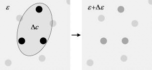
(a)      (b)

Figure 1: Schematic representation of the ABM differential algorithm: (a) addition of a portion of new particles with concentration $\Delta c/(1-c)$ in the particle-void region to the current effective medium with permittivity $\varepsilon$ (the lighter area) leads to (b) the formation of a new effective medium with permittivity $\varepsilon+\Delta\varepsilon$, which serves as the matrix for the next portions of inclusions. Therefore, the previously added portions interact electrically with the new one only via the effective medium (comprising the particles shown darker).

In terms of $\delta\varepsilon$, this assumption can be written as

$$\delta\varepsilon_{\rm ABM}^{(l)}({\bf r}) = (\varepsilon-(\varepsilon+\Delta\varepsilon))[1-{\tilde{\chi}}_{1}({\bf r})-\Delta{\tilde{\chi}}_{1}({\bf r})]$$ (7)

$$+(\varepsilon_{1}-(\varepsilon+\Delta\varepsilon))\Delta{\tilde{\chi}}_{1}({\bf r})$$

$$\approx -\Delta\varepsilon[1-{\tilde{\chi}}_{1}({\bf r})]+(\varepsilon_{1}-\varepsilon)\Delta{\tilde{\chi}}_{1}({\bf r}),$$

where only the terms of the first orders of smallness in $\Delta{\tilde{\chi}}_{1}$ (in the meaning of its average) and $\Delta\varepsilon$ are retained; $\varepsilon$ in (6) also should be changed to $\varepsilon+\Delta\varepsilon$, however it is not necessary for this particular form of $\delta\varepsilon$. Substituting (7) into (6), taking into account the ergodic hypothesis, and using the orthogonality condition $(1-{\tilde{\chi}}_{1}-\Delta{\tilde{\chi}}_{1})\Delta{\tilde{\chi}}_{1}=0$ for the characteristic functions, averaging over the entire system in (6) can be split into averaging over the region occupied by the matrix and averaging over the region occupied by a new portion of inclusions:

$$-\left\langle\frac{\Delta\varepsilon[1-{\tilde{\chi}}_{1}-\Delta{\tilde{\chi}}_{1}]}{3(\varepsilon+\Delta\varepsilon)+\Delta\varepsilon[1-{\tilde{\chi}}_{1}-\Delta{\tilde{\chi}}_{1}]}\right\rangle$$

$$\qquad+\left\langle\frac{(\varepsilon_{1}-(\varepsilon+\Delta\varepsilon))\Delta{\tilde{\chi}}_{1}}{3(\varepsilon+\Delta\varepsilon)+(\varepsilon_{1}-(\varepsilon+\Delta\varepsilon))\Delta{\tilde{\chi}}_{1}}\right\rangle$$

$$\approx-\frac{\Delta\varepsilon}{3\varepsilon}(1-c)+\frac{\varepsilon_{1}-\varepsilon}{2\varepsilon+\varepsilon_{1}}\Delta c=0,$$

where again only the terms of the first order of smallness were retained. Changing to the infinitesimal values $d\varepsilon$ and $dc$ gives the differential equation

$$\frac{dc}{1-c}=\frac{d\varepsilon}{3\varepsilon}\frac{(2\varepsilon+\varepsilon_{1})}{(\varepsilon_{1}-\varepsilon)}.$$ (8)

The point $c=1$ is a critical one; the solution of (8) should satisfy there the condition $\varepsilon=\varepsilon_{1}$. The ABM mixing rule is obtained by integrating the left side of (8) with respect to $c$ from zero to $c$ and the right side with respect to $\varepsilon$ from $\varepsilon_{0}$ to $\varepsilon$:

$$1-c=\frac{\varepsilon-\varepsilon_{1}}{\varepsilon_{0}-\varepsilon_{1}}\left(\frac{{\varepsilon_{0}}}{\varepsilon}\right)^{1/3}.$$ (9)

This equation has the same form as the one for the complex permittivity (the integration is performed then using Morera’s and Cauchy’s theorems Hanai1960 ). As was mentioned in Introduction, this approach is applicable for low concentrations of inclusions (the upper index $l$ in (7) is used to signify this fact).

In a similar way, the high-concentration rule can be obtained. The inclusions are now considered as “the host medium” and the host medium as “the inclusions”, with the characteristic function $\tilde{\chi}_{0}=(1-\tilde{\chi}_{1})$. A portion of “the inclusions” with the characteristic function $\Delta\tilde{\chi}_{0}=-\Delta\tilde{\chi}_{1}$ is embedded into that part of the current effective medium which is void of “the inclusions”; its characteristic function is $(1-\tilde{\chi}_{0}-\Delta\tilde{\chi}_{0})$. Correspondingly,

$$\delta\varepsilon_{\rm ABM}^{(h)}({\bf r}) \approx -[1-{\tilde{\chi}}_{0}({\bf r})]\Delta\varepsilon+(\varepsilon_{0}-\varepsilon)\Delta{\tilde{\chi}}_{0}({\bf r})$$ (10)

$$= -{\tilde{\chi}}_{1}({\bf r})\Delta\varepsilon-(\varepsilon_{0}-\varepsilon)\Delta{\tilde{\chi}}_{1}({\bf r}).$$

Substituting (10) into (6) and taking the necessary integrals give the desired rule:

$$c=\frac{\varepsilon-\varepsilon_{0}}{\varepsilon_{1}-\varepsilon_{0}}\left(\frac{\varepsilon_{1}}{\varepsilon}\right)^{1/3}.$$ (11)

Note that (11) is used rarely, in contrast to the original low-concentration ABM Sen1981 .

3) The Looyenga Looyenga1965 and Lichtenecker Licht1926 rules

$$\varepsilon^{1/3}=(1-c)\varepsilon_{0}^{1/3}+c\varepsilon_{1}^{1/3},$$ (12)

$$\log\varepsilon=(1-c)\log\varepsilon_{0}+c\log\varepsilon_{1},$$ (13)

for low-contrast systems LandauT8 ; Simpkin2010 , can also be obtained by substituting into (6) the formal expressions

$$\delta\varepsilon({\bf r}) = (f(\varepsilon_{0})-f(\varepsilon)){(1-{\tilde{\chi}_{1}({\bf r})})}$$ (14)

$$+(f(\varepsilon_{1})-f(\varepsilon)){\tilde{\chi}_{1}({\bf r})},$$

with $f(x)=\{x^{1/3},\log{x}\}$, respectively, and keeping only the first-order terms in $|f(\varepsilon_{i})-f(\varepsilon)|$ ($i=0,1$). However, these $\delta{\varepsilon}$’s hardly have transparent physical meanings.

III Differential scheme within the CGA

In this section, we develop a general procedure for building differential mixing rules based upon the CGA. The above low- (9) and high-concentration (11) rules turn out to be obtainable from the general differential equation under certain simplifications. In other words, these ABM rules are approximate and of limited usefulness. The general differential equation makes it possible not only to obtain their improved modifications, but also investigate the validity limits for the latter.

Suppose that an infinitesimal addition of inclusions to the system causes the filler concentration and the effective permittivity to change by small $\Delta c$ and $\Delta\varepsilon$, respectively. In view of (4), the new permittivity distribution in the system becomes

$$\widetilde{\delta\varepsilon}_{\rm CGA}({\bf r}) = (\varepsilon_{0}-(\varepsilon+\Delta\varepsilon))[1-({\tilde{\chi}}_{1}({\bf r})+\Delta{\tilde{\chi}}_{1}({\bf r}))]$$ (15)

$$+(\varepsilon_{1}-(\varepsilon+\Delta\varepsilon))[{\tilde{\chi}}_{1}({\bf r})+\Delta{\tilde{\chi}}_{1}({\bf r})],$$

and $\varepsilon$ in (6) changes to ${\varepsilon}+\Delta\varepsilon$. Using simple algebraic manipulations, the expression (15) can be represented as the sum of the distributions (4), (7), and (10):

$$\widetilde{\delta\varepsilon}_{\rm CGA}({\bf r})=\delta\varepsilon_{\rm ABM}^{(l)}({\bf r})+\delta\varepsilon_{\rm ABM}^{(h)}({\bf r})+\delta\varepsilon_{\rm CGA}({\bf r}).$$ (16)

Thus, according to the CGA, any changes in $\varepsilon$ caused by the addition of small amounts of inclusions do not reduce to the contribution from these inclusions alone (the term $\delta\varepsilon_{\rm ABM}^{(l)}$ (7), as in the ABM), but are also influenced by the changes in the host volume fraction (the term $\delta\varepsilon_{\rm ABM}^{(h)}$ (10)) and by the state of the system just before the addition (the term $\delta\varepsilon_{\rm CGA}$ (4)). It follows immediately that the original differential procedures Hanai1960 ; Hanai1980 ; Hanai1986 ; Sen1981 behind the ABM are incomplete.

Substituting (16) into (6) and changing to the infinitesimal values, the differential equation

$$\left[dc\frac{\varepsilon_{1}-\varepsilon}{2\varepsilon+\varepsilon_{1}}-(1-c)\,d\varepsilon\frac{3\varepsilon_{0}}{(2\varepsilon+\varepsilon_{0})^{2}}\right]$$

$$+\left[-dc\frac{\varepsilon_{0}-\varepsilon}{2\varepsilon+\varepsilon_{0}}-c\,d\varepsilon\frac{3\varepsilon_{1}}{(2\varepsilon+\varepsilon_{1})^{2}}\right]=0.$$ (17)

is obtained. Actually, this is the differential form of (5). It is convenient to use (17) to derive new low- and high-concentration modifications of the ABM rules.

Consider first the low concentration limit, where $c$ and $({\varepsilon}_{0}-\varepsilon)$ can be assumed to be of the same order of smallness as $\Delta c$ and $\Delta\varepsilon$ are. Then $\delta\varepsilon_{\rm ABM}^{(h)}$ and the terms in the second brackets in (17) are of the second order of smallness and can be neglected. Correspondingly, $\widetilde{\delta\varepsilon}_{\rm CGA}$ is determined only by the first and third terms in (16):

$$\widetilde{\delta\varepsilon}_{\rm CGA}^{(l)}\approx\delta\varepsilon_{\rm ABM}^{(l)}+\delta\varepsilon_{\rm CGA},$$ (18)

and only the terms in the first brackets in (17) must be retained. This gives the differential equation

$$\frac{dc}{1-c}=d\varepsilon\frac{3\varepsilon_{0}(2\varepsilon+\varepsilon_{1})}{(\varepsilon_{1}-\varepsilon)(2\varepsilon+\varepsilon_{0})^{2}}.$$ (19)

This equation can also be derived by directly substituting (18) into (6), retaining the terms of the first order of smallness, and passing to the infinitesimal increments $dc$ and $d\varepsilon$.

An analogous procedure for the high-concentration limit gives

$$\widetilde{\delta\varepsilon}_{\rm CGA}^{(h)}\approx\delta\varepsilon_{\rm ABM}^{(h)}+\delta\varepsilon_{\rm CGA},$$ (20)

$$\frac{dc}{c}=-d\varepsilon\frac{3\varepsilon_{1}(2\varepsilon+\varepsilon_{0})}{(\varepsilon_{0}-\varepsilon)(2\varepsilon+\varepsilon_{1})^{2}}.$$ (21)

In general, equations (18) and (20) differ considerably from their ABM counterparts (8) and (10), but reduce to them provided the term $\delta\varepsilon_{\rm CGA}$ is neglected. This is possible if: (1) $\varepsilon_{0}\approx\varepsilon$ and $\varepsilon_{1}\approx\varepsilon$, respectively; (2) the concentration of the constituent being added is small; (3) $|\varepsilon_{1}-\varepsilon_{0}|$ is small as well. It follows that the original ABM mixing rules are, in general, physically inconsistent. In practice, one can attempt to apply them only to diluted low-contrast systems.

The equations (19) and (21) are improved differential equations, which partially take into account, through $\delta\varepsilon_{\rm CGA}$, the interaction between the constituent. The integration of them results in the following mixing rules for low and high concentrations of the filler, respectively:

$$\ln{(1-c)} = \frac{9\varepsilon_{0}\varepsilon_{1}}{(2\varepsilon_{1}+\varepsilon_{0})^{2}}\ln{\left[\frac{3\varepsilon_{0}(\varepsilon-\varepsilon_{1})}{(\varepsilon_{0}-\varepsilon_{1})(2\varepsilon+\varepsilon_{0})}\right]}$$ (22)

$$-\frac{2(\varepsilon_{0}-\varepsilon_{1})(\varepsilon_{0}-\varepsilon)}{(2\varepsilon_{1}+\varepsilon_{0})(2\varepsilon+\varepsilon_{0})};$$

$$\ln{c} = \frac{9\varepsilon_{0}\varepsilon_{1}}{(2\varepsilon_{0}+\varepsilon_{1})^{2}}\ln{\left[\frac{3\varepsilon_{1}(\varepsilon-\varepsilon_{0})}{(\varepsilon_{1}-\varepsilon_{0})(2\varepsilon+\varepsilon_{1})}\right]}$$ (23)

$$-\frac{2(\varepsilon_{1}-\varepsilon_{0})(\varepsilon_{1}-\varepsilon)}{(2\varepsilon_{0}+\varepsilon_{1})(2\varepsilon+\varepsilon_{1})}.$$

Compared to the ABM, we expect these rules to be more accurate and valid for wider concentration regions. However, as based on the assumptions (18) and (20), they are still approximate. To prove this fact, consider the Hashin-Shtrikman (HS) upper $\varepsilon^{+}$ and bottom $\varepsilon^{-}$ bounds HS1962

$$\varepsilon^{+}=\varepsilon_{1}+\frac{3(1-c)\varepsilon_{1}(\varepsilon_{0}-\varepsilon_{1})}{3\varepsilon_{1}+c(\varepsilon_{0}-\varepsilon_{1})},$$ (24)

$$\varepsilon^{-}=\varepsilon_{0}+\frac{3c\varepsilon_{0}(\varepsilon_{1}-\varepsilon_{0})}{3\varepsilon_{0}+(1-c)(\varepsilon_{1}-\varepsilon_{0})}.$$ (25)

It is easy to see that the rules (22) and (23) fail to satisfy these bounds (see Fig. 2). Indeed, consider the rule (22) for a system with $\varepsilon_{1}\gg\varepsilon_{0}$. For $c>(1-e^{-1/2})\approx 0.393$, $\varepsilon\to\varepsilon_{1}$, which is higher than the upper HS bound (24) for the same concentrations. In the region of low concentrations (22) is closer to (5) than (9) and falls in between the HS bounds. Similarly, for (23) and $c<e^{-2}\approx 0.135$, $\varepsilon\to\varepsilon_{0}$, which is lower than the HS bottom bound (25).

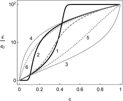
Figure 2: The concentration dependence of $\varepsilon$ according to: the new low- (22) and high-concentration (23) rules (thick solid lines 1 and 2, respectively); Hashin-Shtrikman bottom (25) and upper (24) bounds (thin solid lines 3 and 4); CGA (5) (dashed line); original ABM low- (9) and high-concentration (11) rules (dotted lines 5 and 6). The only parameter used $\varepsilon_{1}/\varepsilon_{0}=10^{2}$.

For arbitrary $\varepsilon_{1}$ and $\varepsilon_{0}$ the concentrations where the HS bounds are violated depend on the contrast $\varepsilon_{0}/\varepsilon_{1}$. Figure  2 illustrates the situation for a system with $\varepsilon_{1}/\varepsilon_{0}=10^{2}$. It is interesting to note that the original ABM rules (9) and (11) satisfy the HS bounds. According to the above discussion, this fact is not indicative of the superiority of the ABM rules (9) and (11) over their modifications (22) and (23), but reflects the changes in the interplay between $\delta{\varepsilon}_{\rm ABM}^{(l)}({\bf r})$, $\delta{\varepsilon}_{\rm ABM}^{(h)}({\bf r})$, and $\delta{\varepsilon}_{\rm CGA}({\bf r})$ in the formation of $\varepsilon$ that occur as $c$ is changed. In other words, a simple extrapolation of the simplifications used within the differential method for one narrow concentration range fails to incorporate the effects essential for the formation of $\varepsilon$ in other concentration ranges.

It should be noted that the above results quantitatively support the well-known qualitative arguments Chelidze ; Chelidze1999 that at high concentrations, both the ABM and Maxwell-Wagner-Hanai models do not fully take into account interparticle polarization effects. They also explain why it is necessary to modify the classical differential models, or even introduce additional adjustable parameters, in order to extend their ranges of applicability Becher1987 ; Sihvola2007 . And they are in accord the final-element calculations Mejdoubi2007 which show that at small concentrations, the small changes of the effective permittivity due to the addition of a new portion of inclusions are greater than those predicted by the differential mixing procedure.

IV Conclusion

The differential approach to the effective permittivity $\varepsilon$ of a system implies that infinitesimal changes in the concentrations of constituents lead to infinitesimal changes in $\varepsilon$; the result is a differential equation for $\varepsilon$. In the present work, we develop a general differential scheme for dielectric systems of impenetrable balls based upon the compact groups approach (CGA). For this purpose, the CGA is formulated in a way that allows one to analyze the role of different contributions to the model permittivity distribution in a system. The analysis of these contributions and corresponding differential equations reveals that:

1. The low- and high-concentration mixing rules of the classical asymmetrical Bruggeman model (ABM) are reproducible within our model under the suggestion that the electromagnetic interaction between the inclusions already contained in the system with those being added can be replaced by the interaction of the latter with the current effective medium. Therefore, the classical ABM mixing rules are, in general, physically inconsistent and applicable only for diluted (with respect to one of the constituents) systems with low dielectric contrast between the constituents.

2. The overall changes in $\varepsilon$ due to addition of an infinitesimal portion of one constituent include the contributions from both constituents (inclusions and the host medium) and depend on the state of the system before the addition. Ignoring the contribution from one of the constituents, we obtain generalized versions of the original ABM mixing rules.

3. The new generalized differential mixing rules are, again, applicable only in certain concentration ranges because beyond those they do not satisfy the Hashin-Shtrikman bounds. This means that different mechanisms are responsible for the formation of $\varepsilon$ in different concentration ranges. Simple extrapolation of the results obtained for a certain concentration range cannot incorporate all the effects essential for the formation of $\varepsilon$ in the whole concentration range.

The results obtained can be generalized to macroscopically homogeneous and isotropic systems with complex permittivities of the constituents. However, it should be emphasized that the novelty of this article is not a derivation of new differential mixing rules, but the quantitative proof of a general statement that differential mixing rules are approximate and applicable only for narrow ranges of concentration and dielectric contrast. Attempts to go beyond those ranges will be, strictly speaking, misleading because of uncontrollable mistakes inherent to the differential method.

Appendix

Appendix A Derivation of equation (6)

The first step is to present the equation

$$\Delta\mathbf{E}(\mathbf{r})-\nabla(\nabla\mathbf{E}(\mathbf{r}))+k_{0}^{2}\epsilon_{0}\varepsilon_{\rm f}\mathbf{E}(\mathbf{r})=-k_{0}^{2}\epsilon_{0}\delta\varepsilon(\mathbf{r})\mathbf{E}(\mathbf{r})$$ (26)

for a wave propagating in the inhomogeneous medium, with local permittivity $\varepsilon({\bf r})=\varepsilon_{\rm f}+\delta\varepsilon({\bf r})$, in the integral form

$$\mathbf{E}(\mathbf{r})=\mathbf{E}_{0}(\mathbf{r})-k_{0}^{2}\epsilon_{0}\int\limits_{V}{d{\mathbf{r}}^{\prime}}{\rm{\hat{T}}}({\mathbf{r}}-{\mathbf{r}}^{\prime})\delta\varepsilon({\mathbf{r}}^{\prime}){\mathbf{E}}({\mathbf{r}}^{\prime}).$$ (27)

Here: $\nabla$ is the del operator; $\Delta$ is the Laplace operator; the integral is taken over the volume $V$ of the system under consideration; ${\bf E}_{0}({\bf r})={\bf E}_{0}\exp{({\rm i}\sqrt{\varepsilon_{\rm f}}{\bf k}_{0}\cdot{\bf r})}$ is a probing field with amplitude $\bf{E}_{0}$ and wave vector ${\bf k}=\sqrt{\varepsilon_{\rm f}}{\bf k}_{0}$ in the medium; $\varepsilon_{\rm f}$ is the permittivity of an unknown background medium, in which each constituent (including the host medium) is embedded; $\rm{\hat{T}}$ is the electromagnetic field propagator (the Green’s tensor for (26)). It can be shown Sushko2004 ; Sushko2007 ; Weiglhofer1995 that $\rm{\hat{T}}$ can be associated with the tensor $\rm{\widetilde{T}}$, such that

$$\int\limits_{V}{d{\bf r}\,{\rm{\hat{T}}}({\bf r})\psi({\bf r})}=\int\limits_{V}{d{\bf r}\,{\rm{\widetilde{T}}}({\bf r})\psi({\bf r})}$$

for “sufficiently good” bounded scalar functions $\psi({\bf r})$. In the long-wave limit ($|{\bf k}|\to 0$), the components of $\rm{\widetilde{T}}$ satisfy the relation

$$k_{0}^{2}\epsilon_{0}{\widetilde{T}}_{\alpha\beta}({\mathbf{r}})={\widetilde{T}}_{\alpha\beta}^{(1)}({\mathbf{r}}) + {\widetilde{T}}_{\alpha\beta}^{(2)}({\mathbf{r}})=\frac{1}{3\varepsilon_{\rm f}}\delta({\mathbf{r}})\delta_{\alpha\beta}$$ (28)

$$+ \frac{1}{4\pi\varepsilon_{\rm f}r^{3}}\left(\delta_{\alpha\beta}-3\frac{r_{\alpha}r_{\beta}}{r^{2}}\right),$$

where $\delta(\mathbf{r})$ is the Dirac delta-function, and $\delta_{\alpha\beta}$ is the Kronecker delta. The part $\rm{\widetilde{T}}^{(1)}$ characterizes the effects of multiple reemissions within compact groups Sushko2007 .

Substituting (28) into (27), making elementary algebraic manipulations, and averaging statistically, we obtain the relation

$$\langle\mathbf{E} (\mathbf{r})\rangle=\left\langle\frac{3\varepsilon_{\rm f}}{3\varepsilon_{\rm f}+\delta\varepsilon({\bf r})}\right\rangle\mathbf{E}_{0}$$ (29)

$$-3\varepsilon_{\rm f}\int\limits_{V}{d{\mathbf{r}}^{\prime}}{\rm{\widetilde{T}}^{(2)}(|{\bf r}-{\bf r}^{\prime}|)\left\langle\frac{\delta\varepsilon({\mathbf{r}}^{\prime})}{3\varepsilon_{\rm f}+\delta\varepsilon({\bf r})}{\mathbf{E}}({\mathbf{r}}^{\prime})\right\rangle}.$$

The local deviation $\delta\varepsilon$ here corresponds to macroscopic compact groups Sushko2007 ; Sushko2009b , not single particles (as in microscopic approaches, such as Stroud75 ; Mackay00 ; Mallet2005 ). For macroscopically isotropic and homogeneous systems, the statistical average in the integrand depends only on $|{\bf r}-{\bf r}^{\prime}|$. Because of this symmetry and a specific angular dependence of $\widetilde{T}_{\alpha\beta}^{(2)}$, the second term in the right-hand side of (29) vanishes, and (29) reduces to

$$\langle{\bf E}({\bf r})\rangle=\xi{\bf E}_{0},\quad\xi=\left\langle{\frac{3\varepsilon_{\rm f}}{3\varepsilon_{\rm f}+\delta\varepsilon({\bf r})}}\right\rangle.$$ (30)

The average displacement $\langle{\bf D}({\bf r})\rangle$ is found using definition (1) and applying the above symmetry reasoning to the $\widetilde{T}_{\alpha\beta}^{(2)}$-involving integral. The result is:

$$\langle{\bf D}({\bf r})\rangle=\epsilon_{0}\varepsilon_{\rm f}\xi{\bf E}_{0}+\epsilon_{0}\langle\delta\varepsilon{\bf E}({\bf r})\rangle=\epsilon_{0}\varepsilon_{\rm f}(1+2\eta){\bf E}_{0},$$ (31)

$$\eta=\left\langle{\frac{\delta\varepsilon({\bf r})}{3\varepsilon_{\rm f}+\delta\varepsilon({\bf r})}}\right\rangle,$$

where it was taken into account that

$$\xi+\eta=1.$$ (32)

Note that by representing (30) and (31) as infinite geometric sequences, we recover the iteration series (2) and (3) Sushko2007 ; Sushko2009b .

Using (1) and taking into account (30), (31), and (32), we obtain

$$\varepsilon-\varepsilon_{\rm f}=(\varepsilon+2\varepsilon_{\rm f})\eta.$$ (33)

In order to find the unknown $\varepsilon_{\rm f}$, we need one more relation between $\varepsilon$ and $\varepsilon_{\rm f}$. We derive it using the equations between the electric field in vacuum and those in the effective and background media:

$${\bf E}_{\rm vac}=\varepsilon\left\langle\bf E\right\rangle,\quad{\bf E}_{\rm vac}=\varepsilon_{\rm f}{\bf E}_{0}.$$

Then

$$\varepsilon_{\rm f}{\bf E}_{0}=\varepsilon\left\langle{\bf E}\right\rangle=\varepsilon\xi{\bf E}_{0},$$

whence, in view of (32),

$$\varepsilon-\varepsilon_{\rm f}=\varepsilon\eta.$$

This and (33) give the relation

$$\eta=\frac{\varepsilon-\varepsilon_{\rm f}}{2\varepsilon_{\rm f}+\varepsilon}=\frac{\varepsilon-\varepsilon_{\rm f}}{\varepsilon}.$$ (34)

Of its two roots $\varepsilon_{\rm f}=0$ and ${\varepsilon}_{\rm f}=\varepsilon$, only the latter is physically meaningful. It corresponds to the well-known Bruggeman-type homogenization and gives the equality $\eta|_{\varepsilon_{\rm f}=\varepsilon}=0$, that is, equation (6).

It should be emphasized that for macroscopically homogeneous and isotropic systems, considered in the long-wavelength limit, the homogenization condition $\varepsilon_{\rm f}={\varepsilon}$ is independent of the functional form of $\delta{\varepsilon}$. The same result was obtained in Sushko2017 by combining the CGA with the Hashin-Shtrikman variational theorem HS1962 . This condition is the key relation postulated in many theories, including the strong-property-fluctuation theory Mackay00 , where it is used to get rid of the secular terms in the Born series for the renormalized electric field.

References

- (1) G. Banhegyi. Comparison of electrical mixture rules for composites. Colloid & Polymer Sci., 264:1030, 1986.
- (2) N. Dudney. Composite electrolytes. Annu. Rev. Mater. Sci., 19:103, 1989.
- (3) C.-W. Nan. Physics of inhomogeneous inorganic materials. Prog. Mater. Sci., 37:1–116, 1993.
- (4) T. Mackay, A. Lakhtakia, and W. Weiglhofer. Strong-property-fluctuation theory for homogenization of bianisotropic composites: Formulation. Phys. Rev. E, 65:6052, 2000.
- (5) M.Ya. Sushko and A.K. Semenov. Conductivity and permittivity of dispersed systems with penetrable particle-host interphase. Cond. Matter Phys., 16(1):13401, 2013.
- (6) A. Shutko and E. Reutov. Mixture formulas applied in estimation of dielectric and radiative characteristics of soils and grounds at microwave frequencies. IEEE Transactions on Geoscience and Remote Sensing, 20:29, 1982.
- (7) F. Bordi, C. Cametti, and T. Gili. Dielectric spectroscopy of erythrocyte cell suspensions. a comparison between looyenga and maxwell-wagner-hanai effective medium theory formulations. Journal of Non-Crystalline Solids, 305:278, 2002.
- (8) S. Nelson. Density-permittivity relationships for powdered and granular materials. IEEE Transactions on Instrumentation and Measurement, 54:2033, 2005.
- (9) D. Bruggeman. Berechnung verschiedener physikalischer konstanten von heterogenen substanzen. i. dielektrizitatskonstanten und leitfahigkeiten der mischkorper aus isotropen substanzen. Ann. Phys., 416:636, 1935.
- (10) D. Bruggeman. Berechnung verschiedener physikalischer konstanten von heterogenen substanzen. i. dielektrizitatskonstanten und leitfahigkeiten der mischkorper aus isotropen substanzen. Ann. Phys., 416:666, 1935.
- (11) T. Hanai. Theory of the dielectric dispersion due to the interfacial polarization and its application to emulsions. Kolloid-Zeitschrift, 171:23, 1960.
- (12) K. Asami, T. Hanai, and N. Koizumi. Dielectric approach to suspensions of ellipsoidal particles covered with a shell in particular reference to biological cells. Jpn. J. Appl. Phys., 19:359, 1980.
- (13) P. Sen, C. Scala, and M. Cohen. A self-similar model for sedimentary rocks with application to the dielectric constant of fused glass beads. Geophysics, 46:781, 1981.
- (14) T. Hanai and K. Sekine. Theory of dielectric relaxations due to the interfacial polarization for two-component suspensions of spheres. Colloid & Polymer Sci., 264:888, 1986.
- (15) K. Wagner. Erklärung der dielektrischen nachwirkungsvorgänge auf grund maxwellscher vorstellungen. Arch. Electrotechn., 2:371, 1914.
- (16) A. Lakhtakia. Incremental maxwell garnett formalism for homogenizing particulate composite media. Microwave and Optical Technology Letters, 17:276, 1998.
- (17) B. Michel, A. Lakhtakia, W. Weiglhofer, and T. Mackay. Incremental and differential maxwell garnett formalisms for bi-anisotropic composites. Composites Science and Technology, 61:13, 2001.
- (18) T. Chelidze, A. Derevjanko, and O. Kurilenko. Electrical spectroscopy of heterogeneous systems. Naukova Dumka, Kiev, 1977.
- (19) D. Bruggeman. Berechnung verschiedener physikalischer konstanten von heterogenen substanzen. ii. dielektrizitatskonstanten und leitfahigkeiten von vielkristallen der nichtregularen systeme. Ann. Phys., 417:645, 1936.
- (20) J. Maxwell-Garnett. Colours in metal glasses and metalic films. Trans. R. Soc. Lond., 203:385, 1904.
- (21) T. Skodvin, J. Sjoblom, J. Saeten, T. Warnheim, and B. Gestblom. A time domain dielectric spectroscopy study of some model emulsions and liquid margarines. Colloids Surfaces A: Physicochem. Eng. Aspects, 83:75, 1994.
- (22) J. Sjoblom, T. Skodvin, Th. Jakobsen, and S. Dukhin. Dielectric spectroscopy and emulsions. a theoretical and experimental approach. J. Dispersion Science and Technology, 15:401, 1994.
- (23) B. Jannier, O. Dubrunfaut, and F. Ossart. Application of microwave reflectometry to disordered petroleum multiphase flow study. Meas. Sci. Technol., 24:025304, 2013.
- (24) R. Pal. Dielectric behavior of double emulsions with ”core-shell droplet” morphology. Journal of Colloid and Interface Sci., 325:500, 2008.
- (25) H. Johnson and E. Poeter. Iterative use of the bruggeman-hanai-sen mixing model to determine water saturations in sand. Geophysics, 70:K33, 2005.
- (26) T. Chelidze and Y. Gueguen. Electrical spectroscopy of porous rocks: a review - i. theoretical models. Geophys. J. Int., 137:1, 1999.
- (27) Z. Yunus, V. Mason, C. Verduzco-Luque, and G. Markx. A simple method for the measurement of bacterial particle conductivities. Journal of Microbiological Methods, 51:401, 2002.
- (28) M.Ya. Sushko. Dielectric permittivity of suspensions. Zh. Eksp. Teor. Fiz., 132:478, 2007. [JETP 105, 426 (2007)].
- (29) M.Ya. Sushko and S.K. Kriskiv. Compact group method in the theory of permittivity of heterogeneous systems. Zh. Tekh. Fiz., 79:97, 2009. [Tech. Phys. 54, 423 (2009)].
- (30) M.Ya. Sushko. Effective permittivity of mixtures of anisotropic particles. J. Phys. D: Appl. Phys., 42:155410, 2009.
- (31) D. Stroud. Generalized effective-medium approach to the conductivity of an inhomogeneous material. Phys. Rev. B, 12:3368, 1975.
- (32) P. Mallet, C. Guerin, and A. Sentenac. Maxwell-garnett mixing rule in the presence of multiple scattering: Derivation and accuracy. Phys. Rev. B, 72:014205, 2005.
- (33) Z. Hashin and S. Shtrikman. A variational approach to the theory of the effective magnetic permeability of multiphase materials. J. Appl. Phys., 33:3125, 1962.
- (34) M.Ya. Sushko. Effective dielectric response of dispersions of graded particles. Phys. Rev. E, 96:062121, 2017.
- (35) S. Tomylko, O. Yaroshchuk, and N Lebovka. Two-step electrical percolation in nematic liquid crystals filled with multiwalled carbon nanotubes. Phys. Rev. E, 92:012502, 2015.
- (36) M.Ya. Sushko, V.Ya. Gotsulskiy, and M.V. Stiranets. Finding the effective structure parameters for suspensions of nano-sized insulating particles from low-frequency impedance measurements. Journal of Molecular Liquids, 222:1051, 2016.
- (37) M. Ya. Sushko. Compact group approach to the analysis of dielectric and optical characteristics of finely dispersed systems and liquids. Journal of Physical Studies, 13(4):4708, 2009.
- (38) M.Ya. Sushko. Molecular light scattering of multiplicity 1.5. Zh. Eksp. Teor. Fiz., 126:1355, 2004. [JETP 99, 1183 (2004)].
- (39) M. Ya. Sushko. Experimental observation of triple correlations in fluids. Cond. Matter Phys., 16:13003, 2013.
- (40) L. D. Landau, E. M. Lifshitz, and L. P. Pitaevskii. Electrodynamics of continuous media., volume 8 of Course of Theoretical Physics. Pergamon, Oxford, 1984.
- (41) H. Looyenga. Dielectric constants of heterogeneous mixtures. Physica, 31:401, 1965.
- (42) K. Lichtenecker. Dielectric constant of natural and synthetic mixtures. Physik. Z., 27:115, 1926.
- (43) R. Simpkin. Derivation of lichtenecker s logarithmic mixture formula from maxwell s equations. IEEE Transactions on Microwave Theory and Techniques, 58:545, 2010.
- (44) B. W. Davis. Encyclopedia of Emulsion Technology: Basic Theory, Measurement, Applications, volume 3. Marcel Dekker Inc., 1987.
- (45) L. Jylhä and A. Sihvola. Equation for the effective permittivity of particle-filled composites for material design applications. J. Phys. D: Appl. Phys., 40:4966, 2007.
- (46) A. Mejdoubi and C. Brosseau. Controllable effective complex permittivity of functionally graded composite materials: A numerical investigation. J. Appl. Phys., 102:094105, 2007.
- (47) W. Weiglhofer and A. Lakhtakia. On singularities of dyadic green functions and long wavelength scattering. Electromagnetics, 15:209, 1995.