Asymptotically Free Theory with Scale Invariant Thermodynamics

Abstract

A recently developed variational resummation technique, incorporating renormalization group properties consistently, has been shown to solve the scale dependence problem that plagues the evaluation of thermodynamical quantities, e.g., within the framework of approximations such as in the hard-thermal-loop resummed perturbation theory. This method is used in the present work to evaluate thermodynamical quantities within the two-dimensional nonlinear sigma model, which, apart from providing a technically simpler testing ground, shares some common features with Yang-Mills theories, like asymptotic freedom, trace anomaly and the nonperturbative generation of a mass gap. The present application confirms that nonperturbative results can be readily generated solely by considering the lowest-order (quasi-particle) contribution to the thermodynamic effective potential, when this quantity is required to be renormalization group invariant. We also show that when the next-to-leading correction from the method is accounted for, the results indicate convergence, apart from optimally preserving, within the approximations here considered, the sought-after scale invariance.

I Introduction

The theoretical description of the quark-gluon plasma phase transition requires the use of nonperturbative methods, since the use of perturbation theory (PT) near the transition is unreliable. Indeed, it has been observed that when successive terms in the weak-coupling expansion are added, the predictions for the pressure fluctuate wildly and the sensitivity to the renormalization scale, $M$, grows (see, e.g., Ref. Trev for a review). Due to the asymptotic freedom phenomenon PT only produces convergent results at temperatures many orders of magnitude larger than the critical temperature for deconfinement. At the same time, the development of powerful computers and numerical techniques offers the possibility to solve nonperturbative problems in silico by discretization of the space-time onto a lattice and then performing numerical simulations employing the methods of lattice quantum chromodynamics (LQCD).

So far, LQCD has been very successful in the description of phase transitions at finite temperatures and near vanishing baryonic densities, generating results aoki that can be directly used for interpreting the experimental outputs from heavy ion collision experiments, envisaged to scan over this particular region of the phase diagram. However, currently, the complete description of compressed baryonic matter cannot be achieved due to the so-called sign problem signpb , which is an unfortunate situation, especially in view of the new experiments, such as the Beam Energy Scan program at the Relativistic Heavy-Ion Collider facility. In this case, an alternative is to use approximate but more analytical nonperturbative approaches. One of these is to reorganize the series using a variational approximation, where the result of a related solvable case is rewritten in terms of a variational parameter, which in general has no intrinsic physical meaning and can be viewed as a Lagrangian multiplier that allows for optimal (nonperturbative) results to be obtained.

In the past decades nonperturbative methods based on related variational methods have been employed under different names, such as the linear delta expansion (LDE) lde , the optimized perturbation theory (OPT) opt ; pms , and the screened perturbation theory (SPT) SPT ; SPT3l . The application of these methods starts by using a peculiar interpolation of the original model. For instance, taking the $\lambda\phi^{4}$ scalar theory as an example, the basic idea is to add a Gaussian term $(1-\delta)m^{2}\phi^{2}$ to the potential energy density, while rescaling the coupling parameter as $\lambda\to\delta\lambda$. One then treats the terms proportional to $\delta$ as interactions, using $\delta$ as a bookkeeping parameter to perform a series expansion around the exactly solvable theory represented by the “free” term, $m^{2}\phi^{2}$. At the end, the bookkeeping parameter $\delta$ is set to its original value $(\delta=1)$, while optimally fixing the dependence upon the arbitrary mass $m$ (that remains at any finite order in such a modified expansion) by an appropriate variational criterion. The idea is to explore the easiness of perturbative evaluations (including renormalization) to get higher order contributions that usually go beyond the topologies considered by traditional nonperturbative techniques, such as the large-$N$ approximation. This technique has been used to describe successfully a variety of different physical situations, involving phase transitions in a variety of different physical systems, such as in the determination of the critical temperature for homogeneous Bose gases beccrit ; bec2 , determining the critical dopant concentration in polyacetylene poly , obtaining the phase diagram of magnetized planar fermionic systems GNmag , in the analysis of phase transitions in general PTopt , in the evaluation of quark susceptibilities within effective QCD inspired models tulio , as well as in other applications related to effective models for QCD Kneur:2010yv . Of course, due to gauge invariance issues, one cannot simply consider a gluonic local mass when applying SPT or OPT to QCD. Nevertheless this procedure can be done in a gauge-invariant manner by applying it on the previously well-defined gauge-invariant framework of Hard Thermal Loop (HTL)HTLorig , and it resummation, HTLpt, was developed over one decade ago htlpt1 ; HTLPT3loop . Recently, this approximation has been evaluated up to three-loop order in the case of hot and dense quark matter HTLPTMU , giving results in reasonable agreement with LQCD for the pressure and other thermodynamical quantities. The SPT method has even been pushed to four-loop order in the scalar $\phi^{4}$ model SPT4l . However, the results of resummed HTLpt exhibit a strong sensitivity to the arbitrary renormalization scale $M$ used in the regularization procedure. This is highly desirable to be reduced if one wants to convert these available high order HTLpt results into much more precise and reliable nonperturbative ones and, likewise, to be consistent with expected renormalization group invariance properties. One could hope that the situation would improve by considering higher order contributions, but exactly the opposite has been observed to occur. As recently illustrated in Refs. htlpt1 ; HTLPT3loop ; HTLPTMU , at three loop order HTLpt predicts results close to LQCD simulations for moderate $T\gtrsim 2T_{c}$ at the “central” energy scale value $M=2\pi T$, such that large logarithmic terms are minimized, but this nice agreement is quickly spoiled when varying the scale even by a rather moderate amount.

A solution to this problem has been recently proposed, by generalizing to thermal theories a related variational resummation approach, Renormalization Group Optimized Perturbation Theory (RGOPT). Essentially the novelty is that it restores perturbative scale invariance at all stages of the calculation, in particular when fixing the arbitrary mass parameter from the variational procedure described above, where it is induced by solving the (mass) optimization prescription consistently with the renormalization group equation. The RGOPT was first developed at vanishing temperatures and densities in the framework of the Gross-Neveu (GN) model JLGN , then within QCD to estimate the basic scale ($\Lambda_{\overline{\rm MS}}$JLQCD1 , or equivalently the QCD coupling $\alpha_{S}$). At three-loop order it gives accurate results JLQCD2 , compatible with the $\alpha_{S}$ world averages. The method has also given a precise evaluation of the quark condensate JLqq . More recently some of the present authors have shown, in the context of the $\lambda\phi^{4}$ scalar model, that the RGOPT is also compatible with the introduction of control parameters such as the temperature jlprl ; jlprd . The RGOPT and SPT predictions for the pressure have been compared, showing how the RGOPT indeed drastically improves over the generic scale dependence problem of thermal perturbation theories at increasing perturbative orders.

We also remark that within more standard variational approaches such as OPT, SPT and HTLpt, the optimization process can allow for multiple solutions, including complex-valued ones, as one considers higher and higher orders. Accordingly, in some cases, one is forced to obtain optimal results by using an alternative criterion, for example, by replacing the variational mass with a purely perturbative screened mass SPT3l ; HTLPT3loop ; HTLPTMU , but at the expenses of potentially loosing valuable nonperturbative information. As shown in Ref. JLGN ; JLQCD2 , the RGOPT may also avoid this serious problem, by requiring asymptotic matching of the optimization solutions with the standard perturbative behavior for small couplings.

Various approaches have been made earlier to improve the higher order stability and scale dependence of thermal perturbation theories. For instance the nonperturbative RG (NPRG) framework (see e.g.  NPRG for the $\phi^{4}$ model) should in principle give exactly scale invariant results by construction, if it could be performed exactly. But solving the relevant NPRG equations for thermal QCD beyond approximative truncation schemes appears very involved. Other more perturbative attempts have been made to improve the perturbative scale dependence of thermodynamical QCD quantities, not necessarily relying on a variational or HTLpt resummation framework: rather essentially using RG properties of standard thermal perturbation theories (see, e.g.,  RG_E0QCD ; RArriola ). Our approach also basically starts from standard perturbative expressions, and perturbative RG properties (which is one advantage since many already available higher order thermal perturbative results can be exploited). But it is very different from the latter approaches, due to the crucial role of the variational (optimization) procedure, rooted within a massive scheme. An additional bonus provided by our procedure, as we will illustrate here, is that some characteristic nonperturbative features are already provided at the lowest (“free gas”) order.

In this work we apply the RGOPT to the nonlinear sigma model (NLSM) in 1+1 dimensions at finite temperatures in order to pave the way for future applications concerning other asymptotically free theories, such as thermal QCD. Apart from asymptotic freedom, the NLSM and QCD have other similarities, like the generation of a mass gap and trace anomaly. In the previous RGOPT finite temperature application jlprd ; jlprl , the numerical results for the pressure were mainly expressed as functions of the coupling, as done in the usual SPT applications to scalar theories. Here, on the other hand, we perform an investigation more reminiscent of typical HTLpt applications to hot QCD (see, e.g., Refs. htlpt1 ; HTLPT3loop ; HTLPTMU ), by mainly concentrating on the (thermodynamically) more appealing $P-T$ plane. Another, more technical but welcome feature of considering the NLSM is that, up to two-loop order, the relevant thermal integrals are simple and exactly known (at least for the pressure and derived quantities), which allows for a rather straightforward study of the full temperature range with our method. As a simple model that has been studied many times before in the context of its critical properties and renormalization group results, the NLSM makes then a perfect test ground for benchmarking the RGOPT when compared to other nonperturbative methods.

It is worth mentioning that for HTLpt applied to QCD at two-loop order and beyond, results HTLPT3loop are only available in the high-$T$ approximation regime, not to mention the rather involved gauge-invariance framework required by the method. At three-loop order the NLSM starts to involve more complicated integrals, but this is beyond the present scope, and two-loop order RGOPT, that we will carry out in the present work, will be enough to illustrate the RGOPT efficiency. Although, to the best of our knowledge, SPT (or its high-$T$ expansion variant more similar to HTLpt) has not been applied previously in the NLSM framework, we found it worth to derive and compare in some detail such SPT/HTLpt results with the RGOPT results in the present model. This is useful in order to emphasize the improvements of RGOPT that are generic enough to be appreciated in view of QCD applications. In this work, we also investigate how the RGOPT performs with respect to other thermodynamical characteristics, like the Stefan-Boltzmann limit and the trace anomaly, among others, which were not investigated in Refs. jlprd ; jlprl .

As we will illustrate, the scale invariant results obtained in the present application give further support to the method as a robust analytical nonperturbative approach to thermal theories. Bearing in mind that the RGOPT is rather recent, we will also perform the basic derivation in a way that the present work may also serve as a practical guide for further applications in other thermal field theories.

This paper is organized as follows. In Sec. II we briefly review the NLSM. Then, in Sec. III, we perform the perturbative evaluation of the pressure to the first nontrivial order and discuss the perturbative scale invariant construction. In Sec. IV we modify the perturbative series in order to make it compatible with the RGOPT requirements. The optimization procedure is carried out in Sec. V for arbitrary $N$ up to two-loop order, where we also derive the large-$N$ approximation, the standard perturbation (PT), and the SPT/HTLpt alternative approaches, also up to two-loop order for comparison. Our numerical results are presented and discussed in Sec. VI, where we compare the previous different approximations as well as the next-to-leading (NLO) order of the $1/N$-expansion warringa , for $N=4$, which is a physically appealing choice beyond the more traditional $N=3$ continuum limit of the Heisenberg model. Then we also compare our RGOPT results with lattice simulation results, apparently only available for $N=3$ giacosa . Finally, in Sec. VII, we present our conclusions and final remarks.

II The NLSM in 1+1-dimensions

The two-dimensional NLSM partition function can be written as nlsmrenorm ; ZJ

$$Z\!=\!\int\!\prod_{i=1}^{N}{\cal D}\Phi_{i}(x)\exp\left[\frac{1}{2g_{0}}\!\!\int\!d^{2}x(\partial\Phi_{i})^{2}\right]\delta(\sum_{i=1}^{N}\Phi_{i}\Phi_{i}-1),$$ (1)

where $g_{0}$ is a (dimensionless) coupling and the scalar field is parametrized as $\Phi_{i}=(\sigma,\pi_{1},...,\pi_{N-1})$. In two-dimensions the theory is renormalizable nlsmrenorm and also, according to the Mermin-Wagner-Coleman theorem mermin ; coleman , no spontaneous symmetry breaking of the global $O(N)$ symmetry can take place (at any coupling value). The action is invariant under $O(N)$ but using the constraint, $\sigma(x)=(1-\pi_{i}^{2})^{1/2}$, in order to define the perturbative expansion, breaks the symmetry down to $O(N-1)$. This is accordingly an artifact of perturbation theory, and truly nonperturbative quantities, when calculable, should exhibit the actually unbroken $O(N)$ symmetry ZJ , as shown by the nonperturbative exact mass gap at zero temperature mgapTBA . Thus the perturbation theory describes at first $N-1$ Goldstone bosons, and one may introduce, for later convenience, an infrared regulator, $m_{0}^{2}$, coupled to $\sigma$. In this case the partition function becomes

$$Z(m)=\int d\pi_{i}(x)\left[1-\pi_{i}^{2}(x)\right]^{-1/2}\exp[-{\cal S}(\pi,m)],$$ (2)

where the (Euclidean) action is ${\cal S}(\pi,m)=\int d^{2}x{\cal L}_{0}$ and, upon rescaling $\pi_{i}\to\sqrt{g_{0}}\pi_{i}$, the bare Lagrangian density is

$${\cal L}_{0}=\frac{1}{2}(\partial\pi_{i})^{2}+\frac{g_{0}(\pi_{i}\partial\pi_{i})^{2}}{2(1-g_{0}\pi_{i}^{2})}-\frac{m_{0}^{2}}{g_{0}}\left(1-g_{0}\pi_{i}^{2}\right)^{1/2}.$$ (3)

The above Lagrangian density can be expanded to order-$g_{0}$ yielding

$${\cal L}_{0}\!=\!\frac{1}{2}\left[(\partial\pi_{i})^{2}+m_{0}^{2}\pi_{i}^{2}\right]+\frac{g_{0}m_{0}^{2}}{8}(\pi_{i}^{2})^{2}+\frac{g_{0}}{2}(\pi_{i}\partial\pi_{i})^{2}-{\cal E}_{0},$$ (4)

where for later notational convenience we designate as ${\cal E}_{0}\equiv m^{2}_{0}/g_{0}$ the field-independent term, originating at lowest order from expanding the square root in Eq. (3). At first, one may think that such field-independent “zero-point” energy term could be dropped innocuously (as is indeed sometimes assumed in the literature makino ). However, as we will examine below it is important to keep this term since it plays a crucial role for consistent perturbative RG properties.

In Euclidean spacetime the Feynman rules of the model can be found, e.g., in refs ZJ ; PSbook . The Euclidean four-momentum, in the finite temperature Matsubara’s formalism kapusta , is $p_{0,Eucl}\equiv\omega_{n}$, where $\omega_{n}=2\pi nT$ are the bosonic Matsubara frequencies $(n=0,\pm 1,\pm 2\cdots)$ and $T$ is the temperature. In this work, the divergent integrals are regularized using dimensional regularization (within the minimal subtraction scheme $\overline{\rm MS}$), which at finite temperature and $d=2-\epsilon$ dimensions, can be implemented by using

$$\int\frac{d^{2}p}{(2\pi)^{2}}\to T\,\hbox{$\sum$}\!\!\!\!\!\!\!\int_{\bf p}\equiv T\left(\frac{e^{\gamma_{E}}M^{2}}{4\pi}\right)^{\epsilon/2}\sum_{n=-\infty}^{+\infty}\int\frac{d^{1-\epsilon}p}{(2\pi)^{1-\epsilon}},$$ (5)

where $\gamma_{E}$ is the Euler-Mascheroni constant and $M$ is the $\overline{\rm MS}$ arbitrary regularization energy scale. At finite temperatures this model has been first studied by Dine and Fischler dine in the context of the PT and also in the large $N$ approximation.

III Perturbative Pressure and Scale Invariance

Figure 1: Feynman diagrams contributing to the perturbative pressure at ${\cal O}(g)$. The first term represents $P_{0}(m_{0})$, the second, $P_{1}(m_{0},g_{0})$, the third term represents the self-energy counterterm $P_{0}^{\rm CT}$ (obtained from expanding $Z_{m}$ to first order in $P_{0}(m_{0}=Z_{m}\,m)$), while the fourth term represents the zero point contribution ${\cal E}_{0}(g_{0})$ to Eq. (6).

Considering the contributions displayed in Fig. 1, one can write the pressure up to order ${\cal O}(g_{0})$ as

$$P=P_{0}(m_{0})+P_{1}(m_{0},g_{0})+{\cal E}_{0}(m_{0},g_{0})+{\cal O}(g_{0}^{2}),$$ (6)

where the (one-loop) zeroth-order term represents the usual free gas type of term and it is given by

$$P_{0}(m_{0})=-\frac{(N-1)}{2}I_{0}(m_{0},T),$$ (7)

where

$$I_{0}(m_{0},T)=T\,\hbox{$\sum$}\!\!\!\!\!\!\!\int_{\bf p}\ln\left(\omega_{n}^{2}+\omega_{\bf p}^{2}\right),$$ (8)

with the dispersion relation, $\omega_{\bf p}^{2}={\bf p}^{2}+m_{0}^{2}$.

At two-loop order the pressure receives the contribution from the ${\cal O}(g_{0})$ term

$$P_{1}(m_{0},g_{0})=-(N-1)\frac{(N-3)}{8}m_{0}^{2}g_{0}I_{1}(m_{0},T)^{2},$$ (9)

where $I_{1}(m_{0},T)=\partial I_{0}(m_{0},T)/\partial m_{0}^{2}$, as well as from the counterterm insertion contributions in the one-loop pressure. To this perturbative order, one has $g_{0}=Z_{g}g\equiv g$ and thus just a mass counterterm insertion contribution in the one-loop pressure to deal with. It leads to a counterterm $P^{\rm CT}_{0}$ that can be readily obtained by replacing $m_{0}=Z_{m}m$ in $P_{0}$ and expanding it up to first-order, $P_{0}(m_{0}=Z_{m}\,m)=P_{0}(m)+P^{\rm CT}_{0}(m,g)$, where explicitly

$$P^{\rm CT}_{0}(m,g)=\frac{(N-1)(N-3)}{8\pi\epsilon}m^{2}gI_{1}(m,T),$$ (10)

upon using hikami ; ZJ (our convention is $d=2-\epsilon$)

$$Z_{m}=1-\frac{g}{8\pi}(N-3)\frac{1}{\epsilon}+{\cal O}(g^{2}).$$ (11)

Then, when performing the sum over the Matsubara’s frequencies within the ${\overline{\rm MS}}$ scheme one obtains for the loop momentum integrals $I_{0}$ and $I_{1}$ appearing in the above expressions, the explicit results

$$I_{0}(m_{0},T)=\frac{m_{0}^{2}}{2\pi}\left\{\frac{1}{\epsilon}+\frac{1}{2}-\ln(\frac{m_{0}}{M})\right.$$

$$\left.+\epsilon\left[\frac{1}{4}+\frac{1}{2}\ln(\frac{m_{0}}{M})\left(\ln(\frac{m_{0}}{M})-1\right)\right]\right\}$$

$$+T^{2}\frac{2}{\pi}J_{0}(m/T),$$ (12)

and

$$I_{1}(m,T) = \frac{1}{2\pi}\left\{\frac{1}{\epsilon}-\ln\left(\frac{m}{M}\right)+\frac{\epsilon}{2}\left[\ln^{2}\left(\frac{m}{M}\right)+\frac{\pi^{2}}{24}\right]\right\}$$ (13)

$$- \frac{1}{\pi}J_{1}(m/T),$$

where, in the above expressions, the thermal integrals $J_{0}(x)$ and $J_{1}(x)$ read, respectively,

$$J_{0}(x)=\int_{0}^{\infty}dz\ln\left(1-e^{-\omega_{z}}\right),$$ (14)

and

$$J_{1}(x)=\int_{0}^{\infty}dz\frac{1}{\omega_{z}\left(1-e^{\omega_{z}}\right)},$$ (15)

where we have defined the dimensionless quantity $\omega_{z}^{2}=z^{2}+x^{2}$, with $z=|{\bf p}|/T$ and $x=m/T$.

Putting all together in Eq. (6), inserting $I_{1}(m,T)$ into Eqs. (9), (10) and expanding to ${\cal O}(\epsilon^{0})$, one may isolate the possibly remaining divergences contributing to the pressure (after mass and coupling renormalization having been performed), as

$$P = -\frac{(N-1)}{2}I_{0}^{\rm r}(m,T)$$ (16)

$$- (N-1)\frac{(N-3)}{8}m^{2}g\left[I_{1}^{\rm r}(m,T)\right]^{2}$$

$$- (N-1)\frac{m^{2}}{(4\pi)\epsilon}\left[1-g\frac{(N-3)}{2(4\pi)\epsilon}\right]$$

$$+ \frac{m^{2}}{g}\,Z^{2}_{m}Z^{-1}_{g},$$

where we have defined the finite quantities

$$I_{0}^{\rm r}(m,T)=\frac{m^{2}}{2\pi}\left[\frac{1}{2}-\ln\left(\frac{m}{M}\right)\right]+T^{2}\frac{2}{\pi}J_{0}(m/T),$$ (17)

and

$$I_{1}^{\rm r}(m,T)=-\frac{1}{2\pi}\ln\left(\frac{{m}}{M}\right)-\frac{1}{\pi}J_{1}(m/T).$$ (18)

Then, renormalizing finally the zero-point energy ${\cal E}_{0}(m_{0},g_{0})$, last term in Eq. (16), gives:

$$\frac{m^{2}}{g}\,Z^{2}_{m}Z^{-1}_{g}=\frac{m^{2}}{g}\,Z^{-1/2}_{\pi}$$

$$=\frac{m^{2}}{g}\,\left(1+\frac{(N-1)}{4\pi\epsilon}\,g-\frac{(N-1)(N-3)}{2(4\pi)^{2}\epsilon^{2}}g^{2}+{\cal O}(g^{3})\right),$$

(19)

where we used the exact NLSM relation nlsmrenorm $Z^{2}_{m}Z^{-1}_{g}=Z^{-1/2}_{\pi}$ with $\pi^{2}_{0}=Z_{\pi}\pi^{2}$ and the two-loop order hikami $Z_{\pi}$ counterterm expression. Accordingly, (19) acts as a vacuum energy counterterm, exactly cancelling the remaining divergences in Eq. (16), so that one can write the renormalized two-loop pressure in the compact form

$$P=\frac{m^{2}}{g}-\frac{(N-1)}{2}\left[I_{0}^{\rm r}(m,T)+\frac{(N-3)}{4}m^{2}g\left[I_{1}^{\rm r}(m,T)\right]^{2}\right].$$ (20)

Before we proceed, we should stress that those vacuum energy (pressure) renormalization features in the $\overline{\rm MS}$-scheme are peculiar to the NLSM: in contrast for a general massive model the vacuum energy (equivalently pressure) is not expected to be renormalized solely from the mass and coupling counterterms, such that one needs additional proper vacuum energy counterterms. Here the latter are provided for free, by retaining consistently the field-independent zero-point energy ${\cal E}_{0}(m_{0},g_{0})$ already present in the Lagrangian. Omitting this term would force to introduce new minimal counterterms (i.e cancelling solely the divergent terms shown explicitly in (19)), however missing thus the finite lowest order $m^{2}/g$ term that remains in the renormalized pressure Eq. (20). Moreover, not surprisingly the latter term is crucial to ensure perturbative RG invariance of the renormalized pressure. More precisely, consider the renormalization group (RG) operator, defined by

$$M\frac{d}{dM}\equiv M\frac{\partial}{\partial M}+\beta\frac{\partial}{\partial g}-\frac{n}{2}\zeta+\gamma_{m}m\frac{\partial}{\partial m}.$$ (21)

Applying the latter to the pressure (zero-point vacuum energy) one has $n=0$, so that one only needs to consider the $\beta$ and $\gamma_{m}$ functions. At the two-loop level,

$$\beta=-b_{0}g^{2}-b_{1}g^{3}+{\cal O}(g^{4}),$$ (22)

and

$$\gamma_{m}=-\gamma_{0}g-\gamma_{1}g^{2}+{\cal O}(g^{3}),$$ (23)

where the RG coefficients in our normalization are hikami :

$$b_{0}=(N-2)/(2\pi),$$ (24)

$$b_{1}=(N-2)/(2\pi)^{2},$$ (25)

$$\gamma_{0}=(N-3)/(8\pi),$$ (26)

$$\gamma_{1}=(N-2)/(8\pi^{2}).$$ (27)

It is now easy to check that applying (21) to Eq. (20) gives

$$M\frac{dP}{dM}={\cal O}(g^{2}),$$ (28)

i.e. RG invariance up to higher order (three-loop here) neglected terms. This is a quite remarkable feature of the NLSM, that one can trace to the nonlinear origin of the mass term in (3) (footprint of the decoupled $\sigma$ field, once expressed in terms of $\pi_{i}$ fields). Accordingly this contribution contains much more than mere $\pi_{i}$ mass terms, in particular the RG properties of the finite remnant $m^{2}/g$ piece in Eq. (20) lead to Eq. (28). In contrast, for other models with linear mass terms (like in the $\phi^{4}$ model typically), the naive (perturbative) vacuum energy generally badly lacks RG invariance, already at lowest order.
To further appreciate these features, suppose now that we had dropped the peculiar NLSM zero-point term ${\cal E}_{0}=m^{2}_{0}/g_{0}$ in (3) from the perturbative calculation of the pressure, which is exactly the situation one generally deals with in other (linear) models, where such terms are simply absent from the start. In this case the remaining divergences in Eq. (16) have to be minimally cancelled by appropriate counterterms. Next applying (21) to the resulting finite pressure Eq. (20) (but now missing the very first term), since $\beta$ and $\gamma_{m}$ are at least of order-$g$, one obtains

$$M\frac{dP}{dM}=-(N-1)\frac{m^{2}}{4\pi}+{\cal O}(g),$$ (29)

which explicitly shows the lack of perturbative scale-invariance, the remnant term being of leading order ${\cal O}(m^{2})$. Such remnant terms generally occur in any massive model and are nothing but the manifestation that the vacuum energy of a (massive) theory has a nontrivial anomalous dimension in general. In this case, to restore RG invariance one needs to add finite contributions, perturbatively determined from RG properties (see e.g. jlprl ; jlprd in the thermal context, or for earlier similar considerations at vanishing temperature, RGinvMS ). Thus (once having minimally renormalized the remaining divergences of the pressure), one is lead to (re)introduce an additional finite contribution in ${\cal E}_{0}$ which, upon acting with the RG operator Eq. (21), precisely compensates the remnant anomalous dimension terms like the lowest order one in Eq. (29). Still pretending to ignore the initially present NLSM ${\cal E}_{0}$ term (or when absent like in other model cases), one can add a finite contribution of the generic form $m^{2}f(g)/g$ (which in minimal subtraction schemes cannot depend explicitly on the temperature, nor on the renormalization scale $M$, since it is entirely determined from (integrating) the RG anomalous dimension). Following jlprd ; jlprl one can write the finite zero-point energy contribution, ${\cal E}_{0}^{\rm RG}$:

$${\cal E}_{0}^{\rm RG}=m^{2}\sum_{k\geq 0}s_{k}g^{k-1},$$ (30)

and determine the coefficients $s_{k}$ by applying (21) consistently order by order. In the present NLSM, one can easily check that it uniquely fixes the relevant coefficients up to two-loop order, $s_{0},s_{1}$, as

$$s_{0}=\frac{(N-1)}{4\pi(b_{0}-2\gamma_{0})}=1,$$ (31)

and

$$s_{1}=(b_{1}-2\gamma_{1})\frac{s_{0}}{2\gamma_{0}}=0,$$ (32)

(which vanishes as $b_{1}=2\gamma_{1}$ in the NLSM).
Thus from perturbative RG considerations, Eq. (30) with (31), (32) reconstructs consistently the NLSM first term of (20), originally present in our original NLSM derivation above. While this derivation was unnecessary for the NLSM, it illustrates the procedure needed for an arbitrary massive model, where such finite vacuum energy terms are generally absent and can be reconstructed perturbatively in such a way. As we will see in Sec IV, the presence of this finite vacuum energy piece induces a nontrivial mass gap solution already at lowest order, in contrast with other related variational approaches. Its presence will be crucial to obtain some essentially nonperturbative features of the model already at lowest order. We remark in passing that the result $s_{1}=0$ (equivalently the original NLSM expression (20)) is a consequence of the peculiar RG properties of the NLSM. We anticipate that this affects the properties of the RGOPT solution at two-loop order, as will be examined below in Sec. V. In other models those perturbative subtraction coefficients are a priori all non-vanishing, as is the case in various other scenarios explored so far JLQCD2 ; JLqq ; jlprl ; jlprd .
To conclude this section, we stress that the vacuum energy terms as in Eq. (30), generally required in massive renormalization schemes based on dimensional regularization, have been apparently ignored in many thermal field theory applications, in particular in the SPT and resummed HTLpt construction htlpt1 ; HTLPT3loop , essentially based on adding a (thermal) mass term. In contrast our construction maintains perturbative RG invariance at all levels of the calculation: first, by considering generically for any model the required perturbative finite subtraction (30) (although already present from the start in the peculiar NLSM case, as above explained). In subsequent step, RG invariance is maintained (or more correctly, restored) also within the more drastic modifications implied by the variationally optimized perturbation framework, as we examine now.

IV RG Optimized Perturbation Theory

To implement next the RGOPT one first modify the standard perturbative expansion by rescaling the infrared regulator $m$ and coupling:

$$m\to(1-\delta)^{a}m,\;\;\;\;g\to\delta g,$$ (33)

in such a way that the Lagrangian interpolates between a free massive theory (for $\delta=0$) and the original massless theory (for $\delta=1$) JLQCD1 . This procedure is similar to the one adopted in the standard SPT/OPT lde ; opt ; SPT or HTLpt applications, except for the crucial difference that within the latter methods the exponent is rather taken as $a=1/2$ (for scalar mass terms) or $a=1$ (for fermion mass terms), reflecting the intuitive notion of “adding and subtracting” a mass term linearly, but without deeper motivations. In contrast, as we will recall now, the exponent $a$ in our construction is consistently and uniquely fixed from requiring the modified perturbation, after performing (33), to restore the RG invariance properties, which generally makes it different from the above linear values $a=1/2$ for a scalar term .

Before we proceed, let us first remark that since the mass parameter is being optimized by using the variational stationary mass optimization prescription lde ; pms ; opt (as in SPT/OPT),

$$\frac{\partial P^{\rm RGOPT}}{\partial m}\Bigr{|}_{m={\bar{m}}}=0,$$ (34)

the RG operator acquires the reduced form

$$\left(M\frac{\partial}{\partial M}+\beta\frac{\partial}{\partial g}\right)P^{\rm RGOPT}=0.$$ (35)

which is indeed consistent for a massless theory.

Then, performing the aforementioned replacements given by Eq. (33) within the pressure Eq. (20), consistently re-expanding to lowest (zeroth) order in $\delta$, and finally taking $\delta\to 1$, one gets

$$P^{\rm RGOPT}_{1L}=-\frac{(N-1)}{2}I_{0}^{\rm r}(m,T)+\frac{m^{2}}{g}(1-2a).$$ (36)

Now to fix the exponent $a$ we require the RGOPT pressure, Eq. (36), to satisfy the reduced RG relation, Eq. (35). This uniquely fixes the exponent to

$$a=\frac{\gamma_{0}}{b_{0}}=\frac{(N-3)}{4(N-2)},$$ (37)

where the first generic expression in terms of RG coefficients coincides with the value found for the similar prescription applied to the scalar $\lambda\phi^{4}$ theory jlprd ; jlprl and also to QCD (up to trivial normalization factors). We indeed recall that, as discussed in Refs. JLQCD1 ; JLQCD2 ; JLqq ; jlprl ; jlprd , the exponent $a$ is universal for a given model as it only depends on the first-order RG coefficients, which are renormalization scheme independent. Furthermore, at zero temperature, Eq. (37) greatly improves the convergence of the procedure at higher orders: considering only the first RG coefficients $b_{0}$ and the $\gamma_{0}$ dependence (i.e., neglecting higher RG orders and non-RG terms), it gives the known exact nonperturbatively resummed result at the very first order in $\delta$ and also at any successive order JLQCD2 . This is not the case for $a=1/2$ (for a scalar model), where the convergence appears very slow, if any.

With the exponent $a$ determined, one can write the resulting one-loop RGOPT expression for the NLSM pressure as

$$P^{\rm RGOPT}_{1L}=-\frac{(N-1)}{2}I_{0}^{\rm r}(m,T)+(N-1)\frac{m^{2}}{(4\pi)gb_{0}}.$$ (38)

In the same way, the two-loop standard PT result obtained in the previous section gets modified accordingly to yield the corresponding RGOPT pressure at the next order of those approximation sequences. After performing the substitutions given by Eq. (33), with $a=\gamma_{0}/b_{0}$ within the two-loop PT pressure Eq. (20), expanding now to first order in $\delta$, next taking the limit $\delta\to 1$, gives

$$P^{\rm RGOPT}_{2L} = -\frac{(N-1)}{2}I_{0}^{\rm r}(m,T)+(N-1)\left(\frac{\gamma_{0}}{b_{0}}\right)m^{2}I_{1}^{\rm r}(m,T)$$ (39)

$$- g(N-1)\frac{(N-3)}{8}m^{2}\left[I_{1}^{\rm r}(m,T)\right]^{2}$$

$$+ \frac{(N-1)}{4\pi}\frac{m^{2}}{g\,b_{0}}\left(1-\frac{\gamma_{0}}{b_{0}}\right).$$

V RG Invariant Optimization and the Mass Gap

To obtain the RG invariant optimized results, as a general recipe at a given order of the ($\delta$-modified) expansion, one expects a priori to solve the mass optimization prescription (dubbed MOP below), Eq. (34), and the reduced RG relation, Eq. (35), simultaneously, thereby determining the optimized $m\equiv{\bar{m}}$ and $g\equiv{\bar{g}}$ “variational” fixed point values JLGN ; JLQCD2 . However, at the lowest nontrivial $\delta^{0}$ order, applying the reduced RG operator (35) to the ($\delta$-modified) one-loop pressure according to (33) with (37), gives a vanishing result, by construction. Therefore, the only remaining constraint that one can apply at this lowest order is the MOP, Eq. (34).

V.1 One-loop RGOPT mass gap and pressure

Considering thus the MOP, Eq. (34), as giving the mass as a function of the other parameters $g,T,M$, it gives a gap equation for the optimized mass ${\bar{m}}(T)$,

$$f_{MOP}^{(1L)}=1-2\pi gb_{0}I_{1}^{\rm r}(m,T)\equiv 0,$$ (40)

or more explicitly, defining $\bar{x}\equiv\bar{m}/T$, and using Eq. (18),

$$\ln\frac{\bar{m}}{M}+2J_{1}({\bar{x}})+\frac{1}{b_{0}\,g(M)}=0.$$ (41)

For $T\neq 0$ Eq. (41) gives an implicit function of $\bar{m}$, due to the nontrivial $m$-dependence in the thermal integral. At $T=0$, Eq. (41) immediately leads to

$${\bar{m}}(0)=M\exp\left(-\frac{1}{b_{0}\,g(M)}\right).$$ (42)

It is instructive to remark that the above optimized mass gap is dynamically generated by the (nonlinear) interactions and reflects dimensional transmutation, with nonperturbative coupling dependence. Accordingly the formerly perturbative Goldstone bosons get a nonperturbative mass, indicating the restoration of the full $O(N)$ symmetry (although within our limited one-loop RG approximation, at least at the same approximation level as the large-$N$ limit ZJ ; warringa ). The Eq. (42) moreover fixes the optimized mass $\bar{m}$ to be fully consistent with the running coupling $g(M)$ as described by the usual one-loop result,

$$g^{-1}(M)=g^{-1}(M_{0})+b_{0}\ln\frac{M}{M_{0}},$$ (43)

in terms of an arbitrary reference scale, $M_{0}$.

Now replacing the mass gap expression, Eq. (41), within the one-loop pressure, Eq. (38), leads to a more explicit and rather simple expression. Namely,

$$P^{\rm RGOPT}_{1L} = -\frac{(N-1)}{\pi}T^{2}\left\{J_{0}\left(\frac{\bar{m}}{T}\right)\right.$$ (44)

$$+ \left.\frac{1}{8}\left(\frac{\bar{m}}{T}\right)^{2}\left[1+4J_{1}\left(\frac{\bar{m}}{T}\right)\,\right]\right\},$$

where $\bar{m}\equiv\bar{m}(g,M,T)$ is given by the solution of Eq. (41) .

For completeness, we also give the corresponding pressure at zero-temperature, that we will use to subtract from Eq. (44) in the numerical illustrations to be given in Sec. VI, such as to obtain a conventionally normalized pressure, $P(T=0)\equiv 0$. From Eq. (44) one obtains

$$P^{\rm RGOPT}_{1L}(T=0)=-\frac{(N-1)}{8\pi}\,\bar{m}^{2}(0),$$ (45)

where the $T=0$ mass-gap is given in Eq. (42).

From the above expressions, one may anticipate that Eqs. (41) and (44) exhibit “exact” scale invariance (of course exact upon neglecting higher order terms at this stage), as it will be further illustrated by the numerical evaluations performed in Sec. VI.

V.2 Large-$N$ mass gap and pressure

Before deriving the RGOPT results at the next (two-loop) order, for completeness we consider the large-$N$ (LN) limit of the model, as it can be directly obtained from the previous one-loop RGOPT result and it will be also studied for comparison purposes in the sequel. The LN limit is straightforwardly generated from the usual procedure of rescaling the coupling as

$$g\equiv g_{LN}/N,$$ (46)

and then taking the limit $N\to\infty$ in the relevant expressions above, such that typically any $(N-1)$, $(N-2)$, $\cdots$ factors in Eq. (38), or previous related expressions reduce to $N$, while higher orders terms are $1/N$-suppressed . Therefore, the LN limit of the RGOPT pressure expression (38) takes the explicit form

$$P^{\rm LN}=-\frac{N}{2}I_{0}^{\rm r}(m,T)+N\frac{m^{2}}{2g_{LN}}.$$ (47)

Note that Eq. (47) is fully consistent with the first order of the nonperturbative two-particle irreducible (2PI) CJT formalism CJT result given in Ref. giacosa (the Eq. (2.42) in that reference), upon further subtracting $P(T=0)$ from Eq. (47), with the large-$N$ limit of the mass gap $\bar{m}$, Eq. (42), $b_{0}\,g\to g_{LN}/(2\pi)$, also consistent with the Eq. (2.44) of Ref. giacosa . The authors of Ref. giacosa have explained the reasons for the strict equivalence of their first order CJT approximation with the large-$N$ results warringa .

The similarities between RGOPT at one-loop order and the first nontrivial order of 2PI results were already noticed in the context of the scalar $\phi^{4}$ model jlprd . Hence, at large-$N$ the rather simple RGOPT lowest (one-loop) order procedure is equivalent to resumming the leading order temperature dependent terms for the mass self-consistently and this result remains valid at any temperature.

Note also that within the standard nonperturbative LN calculation framework, the last term in Eq. (47) arises when this approximation is implemented with, e.g., the traditional auxiliary field method warringa , and is crucial to maintain consistent RG properties. Accordingly, the LN pressure will also exhibit ”exact“ scale invariance, at this approximation level. However, as we will examine explicitly below, the pressure at the NLO in the $1/N$ expansion, although an a priori more precise nonperturbative quantity, is not exactly scale invariant, exhibiting a moderate residual scale dependence.

The LN pressure (47) now scales as $\sim N$. Thus, to compare this LN approximation in a sensible manner with the true physical pressure (i.e. for a given physical $N_{phys}$ value), in the numerical illustrations to be performed in Sec. VI, we will adopt the standard convention to take the overall $N$ factor of the LN pressure (47) as $N\to N_{phys}$ (typically $N_{phys}=3,4,\cdots$ in our numerical illustrations).

V.3 Two-loop RGOPT mass gap and pressure

Going now to two-loop order, the mass optimization criterion Eq. (34) applied to the RGOPT-modified two-loop pressure Eq. (39) can be cast, after straightforward algebra, in the form (omitting some irrelevant overall factors):

$$f_{MOP}^{(2L)}\equiv\left\{3N-5-b_{0}(N-3)\,g\,\left[1+Y+2x^{2}J_{2}(x)\right]\right\}$$

$$\times m\,\left(\frac{1}{b_{0}\,g}+Y\right)=0,$$ (48)

where, we have defined for convenience the following dimensionless quantity (compare with Eq. (18)),

$$Y\equiv\ln\frac{m}{M}+2J_{1}(x)=-2\pi\,I_{1}^{r}(m,T),$$ (49)

and the thermal integral, $xJ_{2}(x)\equiv\partial_{x}J_{1}(x)$ reads

$$J_{2}(x)=\int_{0}^{\infty}dz\frac{[e^{\omega_{z}}(1+\omega_{z})-1]}{\omega_{z}^{3}(1-e^{\omega_{z}})^{2}}.$$ (50)

Alternatively, the reduced RG equation (35), using the exact two-loop $\beta$-function Eq. (22), yields

$$f_{RG}^{(2L)}\equiv m^{2}\,\left[g\frac{(3N-5)}{2\pi}+(N-3)\times\right.$$

$$\left.\left\{1+\frac{N-2}{\pi}g\,Y\left[1+\frac{N-2}{4\pi}g\,(1+\frac{g}{2\pi})\,Y\right]\right\}\right]=0.$$ (51)

When considered as two alternative (separate) equations, (48) and (51), apart from having the trivial solution $\bar{m}=0$, also have a more interesting nonzero mass gap solution, $\bar{m}(g,T,M)$, with nonperturbative dependence on the coupling $g$. It is convenient to solve Eq. (51) first formally as second-order algebraic equations for $Y$, as function of the other parameters, and solving (numerically) the mass gap $\bar{m}(g,T,M)$ using Eq. (49). To get more insight on those implicit self-consistent equations for $m(g,T)$, let us first observe that the MOP Eq. (48) factorizes, with the first factor recognized as the one-loop MOP Eq. (41). Now it is easily seen that the other nontrivial solution, given by cancelling the second factor in Eq. (48), gives at $T=0$ a behavior of the coupling (or equivalently, of the mass gap), asymptotically of the form, when $M\gg m$,

$$g(m,M,T=0)\stackrel{{\scriptstyle M\gg m}}{{\longrightarrow}}\left(\frac{5-3N}{N-3}\right)\,\frac{1}{b_{0}\ln\frac{M}{m}},$$ (52)

which badly contradicts the asymptotic freedom (AF) property of the NLSM, the coefficient of the right-hand-side of Eq. (52) having the opposite sign of AF for any $N>3$. We therefore unambiguously reject this solution , which means that at two-loop order, the correct $g\to 0$ AF-compatible physical branch solution of Eq. (48) for the mass gap is unique and formally the same as the one-loop solution from Eq. (41). But more generally one expects both the mass optimization and the RG solution of (51) to differ quite drastically from the one-loop solution, obviously since incorporating higher order RG-dependence. For the NLSM one also immediately notices that the case $N=3$ is very special, as could be expected, since the two-loop original perturbative contribution in Eq. (20) vanishes. Once performing the $\delta$-expansion at two-loop order, even if that gives extra terms, as can be seen by comparing Eqs. (38) and (39), these also vanish for $N\to 3$, since $\gamma_{0}(N=3)=0$, see Eq. (26). Moreover, if using only Eq. (48), it reduces for $N=3$ to the last factor, identical to the one-loop MOP Eq. (41). Thus, if using the latter MOP prescription for $N=3$, one would only recover the one-loop mass gap solution Eq. (41), which implies no possible improvement from one- to two-loop order. However, using instead the full RG equation Eq. (21), as we will specify below, gives a nontrivial two-loop mass gap solution $\bar{m}(g)$ that is intrinsically different and goes beyond the one-loop solution Eq. (41) even for $N=3$. It thus implies that the final RGOPT pressure, considered as a function of the coupling, $P(\bar{m}(g))$, will nevertheless be different from the one-loop Eq. (44). In that way, even for $N=3$, where the purely perturbative two-loop term cancels, the RGOPT procedure allows a different (and a priori improved) approximation from one- to two-loop order. We will see that those differences between one- and two-loop RGOPT expressions happen to be maximal for $N=3$ (which is intuitively expected since it is the lowest possible physical value for the interacting NLSM). This is a quite sensible feature in view of the fact that we will compare the RGOPT one- and two-loop results with nonperturbative lattice simulations giacosa , which are, however, only available for $N=3$ at present.

Now for $N>3$, in principle it would be desirable to find a simultaneous (combined) solution of Eqs. (48) and (51), such as to obtain the approximate optimal “fixed point” set $\{{\bar{m}},{\bar{g}}\}$, as was done in some $T=0$ models JLGN ; JLQCD1 ; JLQCD2 ; JLqq . For $T\neq 0$ it would leave a given pair $(T,M)$ as the only input parameters. But for the present NLSM, a rather unexpected feature happens: as easily derived, e.g., by solving the correct AF physical solution of Eq. (48) first for $Y$, and substituting in Eq. (51)), after some straightforward algebra the latter readily reduces to

$$g\,m^{2}=0.$$ (53)

Thus, at two-loop order there is no such nontrivial RG and MOP combined solution in the NLSM. This is not an expected result in general for other models, but that one can easily trace back to the specific renormalization properties of the NLSM vacuum energy in $\overline{\rm MS}$-scheme as discussed in Sec. III. (Equivalently the subtraction coefficient $s_{1}$ in Eq. (32) vanishes due to the the peculiar NLSM $b_{1}=2\gamma_{1}$ relations between two-loop RG coefficients for any $N$ . It is thus a peculiar feature of the NLSM, unlikely to occur in a large class of other models. It simply means that at two-loop order the NLSM pressure has a too simple $(m,g)$ dependence to provide such a nontrivial intersecting optimal solution of the two relevant, RG and MOP equations. Nontrivial combined RG and MOP solutions should most likely exist for the NLSM at the next three-loop order, which is however beyond the scope of the present analysis. Therefore, restricting ourselves to the two-loop order for simplicity, for $N>3$ we have to select either Eq. (48), or Eq. (51) to give the mass gap, then fixing the coupling more conventionally from its more standard perturbative behavior. Besides these peculiar NLSM features, the latter prescription is also more transparent to compare with former similar SPT or HTLpt available results for other models, where the (mass) optimization or other used prescriptions only provide a mass gap as a function of the coupling, and the coupling is not fixed by other procedures, thus generally chosen as dictated by the standard (massless) perturbative behavior SPT ; htlpt1 ; HTLPT3loop .

Now Eq. (51) alone happens to have real solutions only at large-$N$, in contrast with Eq. (48), which has real solutions for any $N>2$. But since the correct NLSM AF branch of the mass optimization solution of Eq. (48) behaves accidentally very much like at one-loop order, as explained above, we do not expect to gain much from it when going to the two-loop order. A more promising alternative is to use instead the complete RG equation, which combine Eq. (48) and Eq. (51) in the form (omitting irrelevant overall factors):

$$f_{full\,RG}^{(2L)}\equiv f_{RG}^{(2L)}+2m\,\gamma_{m}f_{MOP}^{(2L)}=0,$$ (54)

where $\gamma_{m}$ consistently includes two-loop ${\cal O}(g^{2})$ terms, see Eq. (23). Not only this contains the maximal RG “information”, in contrast with the simpler mass optimization Eq. (48), but since the RG equation is considered alone, ignoring its possible combination with the mass optimization (34), Eq. (54) is more appropriate than the reduced RG Eq. (51), which is obtained only after using Eq. (34). The input parameters are now $\{T,M,g(M)\}$ and Eq. (54) allows to fix $\bar{m}$. Moreover, Eq. (54) does give real solutions for any value of $N$ and for small to moderately large couplings. In addition, as mentioned above, for the very special case $N=3$ it also gives a mass gap solution that is intrinsically different from the one-loop solution (41), a very welcome feature. (This happens because of the additional coupling dependence within $\gamma_{m}$ in Eq. (54), which turns the otherwise trivial RG solution of Eq. (51) alone, for $N=3$, into a nontrivial solution). All the previous considerations therefore impose Eq. (54) as the most sensible and unique prescription, that we follow from now on. For very strong couplings and $N>3$ the solutions of (54) become complex, nevertheless, if needed, this region can still be explored by solving the less stringent condition given by Eq. (48) .

We emphasize that when using Eq. (54) to determine the optimized pressure results, one may consider that the coupling runs in the way dictated by the standard perturbative approximation. Hence, apart from the one-loop running in Eq. (43), we also need the two-loop running coupling, with exact expression given e.g. in  jlprd , which can be approximated as follows with sufficient accuracy (as long as $g$ remains rather moderate $g\sim{\cal O}(1)$),

$$g^{-1}(M) \simeq g^{-1}(M_{0})+b_{0}L+(b_{1}L)g(M_{0})$$ (55)

$$- \left(\frac{1}{2}b_{0}b_{1}L^{2}\right)g^{2}(M_{0})$$

$$- \left(\frac{1}{2}b_{1}^{2}L^{2}-\frac{1}{3}b_{0}^{2}b_{1}L^{3}\right)g^{3}(M_{0})$$

$$+ {\cal O}(g^{4}),$$

where $L=\ln(M/M_{0})$. As it is standard, one can compare the scale dependence of the different approximations by setting $M=\alpha M_{0}$, where $M_{0}$ is an arbitrary reference scale, and varying $\alpha$ in a given range from Eq. (43) or Eq. (55), at one- and two-loop orders, respectively.

V.4 Comparison with PT pressure and Debye screening pole mass

In order to compare our results with the standard (massless) perturbation theory (PT) in the present NLSM model, it is appropriate to consider the high-$T$ expansion of the relevant expressions. This is also relevant for a (merely qualitative) comparison with HTLpt results htlpt1 in other models, since the latter proceeds with expansions in powers of $x=m/T$. We will see in this subsection that Eqs. (41), or equivalently, Eqs. (48) and (54) at two-loop order, have relatively simple mass gap solutions given in this case as a systematic perturbative expansion in powers of the coupling.

It is thus useful to consider the well known high-$T$ expansions, where $x=m/T\ll 1$, for the thermal integrals kapusta ,

$$J_{0}(x)=-\frac{\pi^{2}}{6}+\frac{\pi}{2}x+\left(\frac{x}{2}\right)^{2}\left[\ln\left(\frac{xe^{\gamma_{E}}}{4\pi}\right)-\frac{1}{2}\right]+{\cal O}(x^{4}),$$

(56)

$$J_{1}(x)=-\frac{\pi}{2x}-\frac{1}{2}\,\ln\left(\frac{xe^{\gamma_{E}}}{4\pi}\right)+{\cal O}(x^{4}).$$ (57)

We also introduce the Stefan-Boltzmann (SB) limit of the renormalized NLSM pressure, which will enter as a reference pressure in many of the numerical examples to be given below in Sec. VI,

$$P_{\rm SB}=(N-1)\frac{\pi}{6}T^{2},$$ (58)

which is obtained by taking the massless, or high-$T$ limit, of Eq. (56) of the one-loop perturbative result Eq. (7). This gives for the one-loop RGOPT pressure Eq. (44),

$$\frac{P^{\rm RGOPT}_{1L}}{P_{SB}}=1-\frac{3}{\pi}{\bar{x}}-\frac{3}{2\pi^{2}}{\bar{x}}^{2}\left[L_{T}-\frac{1}{b_{0}\,g}\right]+{\cal O}({\bar{x}}^{4}),$$ (59)

where we have defined $L_{T}=\ln[Me^{\gamma_{E}}/(4\pi T)]$.

Next, the optimized mass solution, obtained from Eq. (41), can be expressed as function of the coupling:

$$\bar{x}\equiv\frac{\bar{m}}{T}=\frac{\pi\,b_{0}g(M)}{1-b_{0}g(M)\,L_{T}},$$ (60)

or that simply gives, when expanding to the lowest perturbative order,

$$\bar{m}(T)\simeq\pi\,b_{0}\,g(M)T+{\cal O}(g^{2}).$$ (61)

Note that using the optimized mass gap solution (60) within Eq. (59), the latter takes a much simpler expression (in the high-$T$ limit here considered),

$$\frac{P^{\rm RGOPT}_{1L}}{P_{SB}}=1-\frac{3}{2\pi}{\bar{x}}+{\cal O}({\bar{x}}^{4})$$

$$\simeq 1-\frac{3}{2}\,\frac{b_{0}g(M)}{1-b_{0}g(M)\,L_{T}}=1-\frac{3}{2}\,b_{0}g(\frac{4\pi T}{e^{\gamma_{E}}}),$$ (62)

using Eq. (43) in the last term. At the next two-loop order, one obtains in the high-$T$ approximation a relatively compact expression of the RGOPT pressure Eq. (39):

$$\frac{P^{\rm RGOPT}_{2L}}{P_{SB}}=1-\frac{3\bar{x}}{4\pi}(\frac{3N-5}{N-2})(1-\frac{\bar{x}}{(N-2)\,g})$$

$$-\frac{3\bar{x}^{2}}{4\pi^{2}}(\frac{N-1}{N-2})\,L_{T}-\frac{3g(N-3)}{16\pi^{3}}\left(\pi+L_{T}\,\bar{x}\right)^{2},$$ (63)

where the correct (i.e. AF) solution $\bar{m}\equiv\bar{x}T$ of the full RG Eq. (54) is given simply by one of the roots of a quadratic equation. $\bar{m}$ is in general different from the one-loop solution (60), as expected since it now involves two-loop order RG coefficients $b_{1},\gamma_{1}$: indeed it has a rather involved dependence on $g$ that we refrain to give explicitly. But once perturbatively re-expanded, it coincides at first order with (60) (for any $N>3$), which is a nontrivial perturbative consistency check of our construction. Replacing this exact two-loop $\bar{m}$ as a function of $g$ within the two-loop pressure (63), one obtains an expression that differs from the one-loop pressure, Eq. (62), by higher order perturbative terms, starting at ${\cal O}(g^{3})$:

$$\frac{P^{\rm RGOPT}_{2L}}{P_{SB}} = 1-\frac{3}{2}\,\frac{b_{0}g(M)}{1-b_{0}g(M)\,L_{T}}$$ (64)

$$+ \frac{3\,g^{3}(M)}{\pi^{3}}\,\frac{(N-2)^{4}}{(N-3)^{2}(3N-5)}+{\cal O}(g^{4}),$$

valid strictly only for $N>3$. Accordingly the extra terms in Eq. (64) illustrate rather simply (perturbatively) the additionnal contributions from two-loop RGOPT with respect to the one-loop pressure (62). One should keep in mind, however, that the exact two-loop pressure (39), including full $g$- and $T$-dependence from the exact $\bar{m}(g,T)$ (which we illustrate numerically below mainly for $N=4$) has a much more involved, nonperturbative dependence on the coupling (and temperature). In particular, while Eq. (64) is a relatively good approximation for moderate $g$ and $N\geq 4$, it is not valid for the very special case $N=3$, for which the exact pressure $P(\bar{m}(g))$ actually does not show any singular behavior, since both the original expression Eq. (63) and $\bar{m}(g)$ are regular for $N=3$. The singularity at $N=3$ seen in Eq. (64) is thus unphysical, being only an artifact of having perturbatively reexpanded $\bar{m}(g)$, which exhibits a $1/(N-3)$ terms at order $g^{2}$. (Therefore for the case $N=3$ some care is needed in the numerics to take the limit $N\to 3$ before possibly expanding in perturbation, which is however not needed). Still, Eq. (64) indicates crudely that the difference between one- and two-loop RGOPT should be maximal for $N=3$, which is also true for the exact (regular) expression, and was intuitively expected, since $N=3$ is the lowest physically nontrivial value. At the other extreme for $N\to\infty$, one can easily check that the two-loop optimized mass and pressure tend towards the corresponding one-loop quantities, i.e. the LN results like the pressure Eq. (47).

To compare the previous RGOPT results with the standard PT ones, one can start by deriving the PT pressure directly from Eq. (20) in the massless limit, which at this two-loop order is well defined. It gives

$$\frac{P^{\rm PT}}{P_{SB}}=1-\frac{3}{2}\,\gamma_{0}\,g(M)+{\cal O}(g^{2}).$$ (65)

Another quantity of interest is the purely perturbative thermal Debye (pole) mass: at one-loop order it can be derived starting from the self-energy nlsmrenorm ; ZJ ,

$$\Gamma^{(2)}(p^{2})=p^{2}(1+g_{0}I_{1})+m^{2}_{0}\left[1+\frac{(N-1)}{2}g_{0}I_{1}\right]+{\cal O}(g^{2})\,,$$ (66)

where $I_{1}$ is the (Euclidean) one-loop integral given by Eq. (13) in $\overline{\rm MS}$ renormalization scheme, with the thermal part $J_{1}(x)$ having the high-$T$ expansion (57). Taking, thus, the pole mass $p^{2}\equiv-m^{2}_{D}$ in Eq. (66), after mass renormalization, it gives, in the massless limit $m\to 0$ relevant for the pure thermal one-loop mass, the result

$${m^{1L}_{D}}=\frac{N-3}{8}\>g(M)\>T\equiv\pi\,\gamma_{0}\,g(M)\>T.$$ (67)

Equation (67) can be contrasted with the more nonperturbative RGOPT result (61). Accordingly, note that the RGOPT optimized mass (61) appears to have a different perturbative behavior than the Debye pole mass (67): Namely, with $\gamma_{0}\to b_{0}$, and similarly for the pressure, comparing the RGOPT result Eq. (59) with the PT pressure (65), the slopes of both masses at the origin as a function of $g$ are different. However, one should not be surprised by these differences. First, in contrast with the physical one-loop Debye (pole) mass, the optimized mass (61) is only an intermediate unphysical quantity in the optimization procedure, aimed to enter the final pressure to make it a (nonperturbative) function of $g$ only. Second, the resulting $P^{\rm RGOPT}(g)$, obtained by such a construction, has a priori more nonperturbative content. Thus, it has no reason to generate a function that exactly matches the one generated by the standard PT. This is similar to the fact that the pressure, in the nonperturbative LN approximation, also is a function of $g$ that is intrinsically different from the purely PT pressure,

$$\frac{P^{\rm LN}}{P_{SB}}=\frac{N}{N-1}\left(1-\frac{3}{2}g_{LN}\right)+{\cal O}(g^{2}_{LN}).$$ (68)

Thus, at this stage the coupling value is an essentially arbitrary input, being not fixed from a physical input at a given scale, in both PT, LN and RGOPT approximation cases, and a physical input would fix a priori different values of the coupling in different approximation schemes. However, the perturbative and physical consistency of the RGOPT pressure result can be checked by appreciating that, once the arbitrary mass in Eq. (59) is replaced with the physical thermal mass $m_{D}$ Eq. (67), one consistently recovers the standard PT pressure as function of $g$, Eq. (65). In other words, when expressed in terms of physical quantities (like here the Debye pole mass) the RGOPT results are consistent with standard PT for $g\to 0$ (see, e.g., Ref. jlprd for a detailed discussion of similar results for the scalar $\phi^{4}$ model).

V.5 Comparison with standard SPT/OPT

For completeness, let us review how the more standard OPT (or SPT) approximation is obtained and derive it for the NLSM, for useful comparison purpose with the RGOPT results. In this case, one starts back again with Eq. (6), but as already emphasized above, there are two important differences with the previously derived RGOPT construction. First, the standard SPT/OPT, as was considered in various models, generally ignored the finite vacuum energy subtraction terms like in Eq. (30), required to restore the perturbative RG invariance as we have discussed. The second difference regards the Gaussian term when performing the interpolation, Eq. (33), since in the standard OPT case the exponent $a$ is fixed in an ad hoc way as $a=1/2$. While it should be clear from the above RGOPT construction that such prescription will therefore lack explicitly RG invariance, we nevertheless follow exactly the procedure as it was applied in various other models, to illustrate the differences in properties of corresponding thermodynamical quantities as compared to the RGOPT, in particular concerning their residual scale dependence.

It is thus straightforward to obtain the SPT/OPT two-loop pressure from the RGOPT result, Eq. (39): upon first omitting the finite contribution to ${\cal E}_{0}$, given by the last term in Eq. (39), furthermore upon replacing the RGOPT exponent $a=\gamma_{0}/b_{0}$ by the standard $a=1/2$ in the second term. These modifications lead to

$$P^{\rm SPT}_{2L} = -\frac{(N-1)}{2}I_{0}^{\rm r}(m,T)+\frac{(N-1)}{2}m^{2}I_{1}^{\rm r}(m,T)$$ (69)

$$- g(N-1)\frac{(N-3)}{8}m^{2}\left[I_{1}^{\rm r}(m,T)\right]^{2}.$$

One should first appreciate that, contrary to the RGOPT case, the SPT/OPT does not provide a non-trivial (i.e. coupling-dependent) optimized mass gap result when only the (one-loop) quasi-particle contribution, given by the first two terms on the right-hand-side of Eq. (69), is accounted for. This is a general feature, not specific to the NLSM. Applying thus the mass optimization Eq. (34) to the complete two-loop $P^{\rm SPT}_{2L}$ result, one obtains a second-order equation quite analogous to Eq. (48),

$$f_{SPT}^{(2L)}=\left[1-\gamma_{0}\,g(1+Y)\right]-2\gamma_{0}\,gx^{2}J_{2}(x)=0,$$ (70)

where the quantity $Y$ was defined in Eq. (49). However, this equation has no real solution for any $N$. Moreover, upon taking its high-$T$ approximation, it gives an unphysical solution, as it no longer depends on the mass. This last feature is an unusual situation within the SPT/OPT/HTLpt applications since, at least for other models considered in the literature, these approximations often provide real results at the first nontrivial order. And, in particular, they usually recover the LN result when $N\to\infty$ optLN as, for example, in the case of the $\lambda\phi^{4}$ scalar theory optON ; OPT3l . In this situation, a frequently used alternative prescription to nevertheless define a mass in SPT (or similarly HTLpt) HTLPT3loop is to employ the purely perturbative NLSM Debye pole mass, as given by Eq. (67). Since we are interested in the complete temperature range and not solely in the high-$T$ regime, we could rather derive ${\bar{m}}_{SPT}$ as the solution of the full one-loop self-consistent mass gap equation obtained from Eq. (66),

$$\bar{m}\equiv\lim_{m\to 0}m\left[1+2\pi\gamma_{0}\,g\,I_{1}^{\rm r}(\bar{m},T)+{\cal O}(g^{2})\right].$$ (71)

But, at this perturbative order, the physical solution of Eq. (71) is nothing but the high-$T$ one-loop Debye mass $m_{D}$, already given in Eq. (67).

For completeness and later use, we also give the expression of the two-loop SPT pressure Eq. (69) in the high-$T$ approximation, upon using its mass-gap solution Eq. (67), therefore becoming only a function of $g(M)\sim g(T)$,

$$\frac{P^{\rm SPT,highT}_{2L}}{P_{SB}}=1-\frac{3}{2}\gamma_{0}g-\frac{3}{2}\gamma_{0}g\left(1+\gamma_{0}gL_{T}\right)^{2}.$$ (72)

In particular, the previous expression is more appropriate for a (very qualitative) comparison with the two-loop HTLpt QCD (pure gluodynamics) pressure HTLPT3loop , which is only available in the small $m/T$ (high-$T$) expansion approximation.

VI Numerical Results

Before proceeding to numerical comparisons of the different approximation methods previously considered, we should specify how to fix the relevant input parameters, which we discuss next.

VI.1 Input parameter choice

As already mentioned, at this stage the coupling $g$ in all previous RGOPT, PT, SPT approximations of the pressure is to be considered an arbitrary input. Ideally, if we had experimental data for some physical observable, like for other models, we could fix $g$ typically at some scale and/or temperature. Accordingly it is clear that the resulting $g(T)$ values would be a priori different within different approximations. Specially, since the LN approximation necessarily implies to rescaling the coupling, Eq. (46), the rescaled coupling $g_{LN}$ value could be substantially different from those for other approximations, for the same observable input given at some physical scale for a finite $N$ value. Now, apart from comparing with other available nonperturbative results (like the NLO $1/N$ expansion warringa or lattice simulations for $N=3$giacosa ), our purpose is also mainly to illustrate the RGOPT scale dependence improvement as compared to the standard PT and the SPT approximation. For the latter comparison it is more sensible to compare scale dependences of the different results for the same “reference” coupling values. But since we also compare the different thermodynamical quantities with the LN ones, one aims to choose $g_{LN}$ input values in a range that is a priori comparable with other approximations. It is clear from Eq. (44) and (47) that the one-loop RGOPT and LN approximations are essentially equivalent, only up to a rescaled coupling (46): indeed, the correct LN result was derived from Eq. (44). Thus we find it sensible to compare the results for a given finite $N_{phys}$ input by taking

$$g_{LN}(M_{0})\simeq(N_{phys}-2)g(M_{0})$$ (73)

When satisfying exactly this relation, the LN and (one-loop) RGOPT describe essentially the same physics: if one would fix $g(M_{0})$ for the different approximations by comparing those to real data, one would expect to obtain something close to Eq. (73), except for the other difference being the $N-1\to N$ overall factor in the LN pressure . Concretely, the numerical illustrations below will be mainly for the case of $N_{phys}=4$, $g(M_{0})=1=g_{LN}(M_{0})/2$, where $M_{0}$ is the arbitrary reference scale, or for $N_{phys}=3$, $g(M_{0})=g_{LN}(M_{0})$ when comparing with the lattice results.

To investigate and compare the scale variation behavior of the different approximations in our analysis below, as it is customary, we set the arbitrary $\overline{\rm MS}$ scale as $M=\alpha M_{0}=2\pi T\alpha$ and consider $0.5\leq\alpha\leq 2$ as representative values of scale variations. Note however that this formal identification of the arbitrary renormalization scale $M$ with a temperature is only justified strictly at high temperature Trev , while the genuine nonperturbative arbitrary $T$-dependence of the coupling is in general not known. Accordingly for the SPT Eqs. (69), (72) and PT Eq. (65), we impose the standard prescription $g(M\sim 2\pi T)$ with the running dictated e.g. at one-loop by Eq. (43). This guarantees the correct SB limit of (65) and Eq. (72) at very high $T$, and is often adopted in the literature even for relatively low $T$ values. In contrast for the RGOPT pressures Eqs. (38) or Eq. (39), the running $g(M\sim T)$ as dictated by Eqs. (43), (55) is consistently embedded (although only approximately at two-loops), as is explicit e.g. from Eq. (62) in the high-$T$ approximation. This is a consequence of the (perturbative) RG invariance-restoring subtraction terms in the pressure expressions, and it automatically gives the SB limit at (very) high $T$. Alternatively, as already emphasized previously, if a nontrivial combined RG and MOP solution of Eq. (48) and (51) would be available at the two-loop order in the present model (which unfortunately is not the case), this solution would effectively provide an approximate “nonperturbative” ansatz for the $T$-dependent coupling, likely departing much from Eqs. (43), (55) at low $T$.
Having previously derived that the one-loop RGOPT (and LN similarly) pressure is exactly scale invariant for any coupling value, we will illustrate the moderate residual scale dependence at the two-loop RGOPT order and those of the other approximation schemes, for a moderately nonperturbative coupling choice, $g(M_{0})\simeq 1$. It is clear that due to the perturbative running, for a very large input coupling the scale dependence drastically increases (except for the one-loop RGOPT result being exactly scale invariant for any $g$) and, thus, the choice $g(M_{0})\simeq 1$ appears to be a reasonable compromise. Note that in the two-dimensional NLSM, a coupling of order $g(M_{0})\simeq 1$ may be naively compared with a relatively strong four-dimensional QCD coupling $\alpha_{S}\sim 1$, which is well within the nonperturbative $T\sim T_{c}$ QCD regime.

VI.2 The $T=0$ results

We start by considering the optimization solutions at $T=0$ and $N=4$.

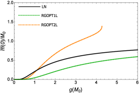
Figure 2: Normalized zero temperature optimized masses, ${\bar{m}}(0)/M_{0}$, as a function of $g(M_{0})$, for $N=4$ and at the central reference scale $\alpha=1$, in the RGOPT at one- and two-loops and in the LN approximations.

In Fig. 2 we compare for $N=4$ the optimized mass ${\bar{m}}(0)$ obtained with the one-loop RGOPT solution from (34), given explicitly by Eq. (42) in the $T\to 0$ limit, with the similar $T\to 0$ two-loop RG solution of $f_{full\,RG}^{(2L)}$ given by Eq. (54), and the LN mass, as functions of the renormalized coupling at the central reference scale $\alpha=1$. (The $T=0$ mass gap for the SPT is not shown as it is trivially vanishing from Eq. (71)). The results in Fig. 2 show that at one-loop order the RGOPT has real solutions for all values of $g$. In contrast, the two-loop RGOPT mass, using $f_{full\,RG}^{(2L)}$, Eq. (54), becomes complex beyond a rather high coupling value, for $N=4$, $g(M_{0})\approx 4.27$, which is a value high enough for our purposes. This $g$ value, beyond which the RG solution is complex, slightly decreases as $N$ increases, but for $N=3$ one recovers a real solution for any $g$. It can be verified that Eq. (54) gives actually two branch solutions. We select unambiguously the one which correctly reproduces the SB result as the physical solution in all subsequent evaluations. That is, as already mentioned concerning the other solution from the mass optimization, Eq. (48), our criterion to select $\bar{m}$ is to choose the root which reproduces the perturbative results for small $g$. The other nonphysical solution, not shown in Fig. 2, has an anti-AF behavior, similarly to the other nonphysical solution of Eq. (48), which is given by Eq. (52). (NB the (real part of the) physical branch solution is not plotted beyond the coupling value where it starts to be complex, that is why it appears to end abruptly).

VI.3 The $T\neq 0$ results

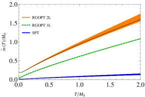
Figure 3: Thermal masses as a function of the temperature (both quantities normalized by the reference scale $M_{0}$) for scale variations $0.5\leq\alpha\leq 2$, $N=4$ and $g(M_{0})=g_{LN}(M_{0})/2=1$. We compare the results for the RGOPT (one- and two-loop cases) and the SPT. (NB for this coupling choice the LN thermal mass is identical to the RGOPT one-loop one). Within the two-loop RGOPT and SPT, the shaded bands have the lower edge for $\alpha=0.5$ and the upper edge for $\alpha=2$. The thin line inside the shaded bands is for $\alpha=1$.

When considering the finite temperature case, we show in Fig. 3 the one-loop RGOPT mass gap from Eq. (41), the two-loop similar result from Eq. (54), which now are functions of the temperature, fixing $g(M_{0})=1$ and varying the scale $M=\alpha M_{0}$, with $0.5\leq\alpha\leq 2$, corresponding to the shaded bands in Fig. 3. We then see from Fig. 3 that the one-loop RGOPT mass is exactly scale independent, as it was anticipated from its expression, given by Eq.(41) in the previous section. This is the case because, by construction, it satisfies both the RG and the OPT equations simultaneously, Eqs. (35) and (34), respectively, which lead to Eq. (41). The two-loop RGOPT and SPT appear, however, not scale invariant. The reasons for this are as follows. First, the residual scale dependence of the SPT mass is not surprising, since its construction lacks RG invariance from the beginning, as already explained previously. Here this is very screened by the smallness of the perturbative mass Eq. (67) used for SPT. While the two-loop RGOPT mass residual scale dependence has a different origin: because the (perturbatively RG-invariant by construction) mass obtained from any of the possible defining Eqs.(48) or (54), for arbitrary temperature, cannot match exactly the running of the coupling Eq. (55), dictated by the purely perturbative behavior at zero-temperature. Note that the scale dependence indeed increases for increasing $T/M_{0}$ in Fig. 3 (but this is artificially enhanced by showing $\bar{m}\sim T$ rather than $\bar{m}/T$, which rather decreases with $T$). The two-loop RGOPT scale dependence appears much larger than the SPT one, but this is essentially due to the intrinsically much larger $\bar{m}/T$ values in the RGOPT than in the SPT case, therefore within the $\bar{m}/T>1$ regime for intermediate $T/M_{0}$, where the implicitly high-$T$ regime justifying the use of the perturbative running (55) is no longer quite valid. However, as we will see below, this sizable scale dependence of the RGOPT mass gets largely damped within the RGOPT pressure, giving an overall scale dependence much more moderate than for the SPT pressure.

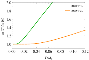
Figure 4: The normalized thermal optimized masses, ${\bar{m}}(T)/{\bar{m}}(0)$, as a function of the temperature $T$ (normalized by $M_{0}$) for $N=4$, $g(M_{0})=1=g_{LN}(M_{0})/2$, and at the central scale choice $\alpha=1$, in the RGOPT at one- and two-loop cases. (NB for this coupling choice the LN thermal mass is identical to the RGOPT one-loop one).

The RGOPT mass ${\bar{m}}(T)$ clearly starts from a nonzero value at $T=0$, since the mass gap solution is nontrivial at $T=0$ (Eq. (42)), then bends and reaches, as expected by using basic dimensional arguments, a straight line for large temperatures, where it behaves perturbatively as $\bar{m}\sim gT$. As observed in Ref. giacosa , this behavior is reminiscent of that of the gluon mass in the deconfined phase of Yang-Mills theories YM1 ; YM2 ; YM3 , where, at high-$T$, the gluon mass can be parametrized by $T/\ln T$. The bending of the thermal masses can be better appreciated in Fig. 4, which shows that the changing of behavior occurs at rather low temperatures.

One should recall, as already emphasized, that $\bar{m}$ is only used at intermediate steps and does not represent a direct physical observable (see Refs. jlprd ; jlprl for further discussions on this issue). In this framework, physical quantities, like the pressure, are obtained upon substituting into these $\bar{m}(g)$, which carries the nonperturbative coupling dependence. Next, we compare the results for the pressure obtained from the different schemes considered, namely, the RGOPT, PT, SPT and LN.

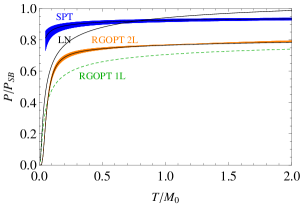
Figure 5: $P/P_{\rm SB}$ as function of the temperature $T$ (normalized by $M_{0}$) for $N=4$ and $g(M_{0})=1=g_{LN}(M_{0})/2$, with scale variation $0.5\leq\alpha\leq 2$. Within the two-loop RGOPT and SPT, the shaded bands have the lower edge for $\alpha=0.5$ and the upper edge for $\alpha=2$. The thin line inside the shaded bands is for $\alpha=1$. (NB the line thickness of one-loop RGOPT and $LN$ is only for visibility at the figure scale and does not correspond to any actual scale dependence since those approximations are exactly scale invariant.)

In Fig. 5 we show the (subtracted) pressure, $P=P(T)-P(0)$, normalized by $P_{\rm SB}$, for the scale variations $M=\alpha M_{0}$, $0.5\leq\alpha\leq 2$ and $N=4$. It illustrates how the one-loop RGOPT pressure is exactly scale invariant, while the two-loop result displays a (small) residual scale dependence for the reasons already discussed above when considering the mass and concerning the interpretation of the results shown in Fig. 3. Note that despite the fact that the optimum mass ${\bar{m}}(T)$ has a non negligible scale dependence for the RGOPT two-loop case, even compared to SPT, the RGOPT pressure itself exhibits a substantially smaller scale dependence than the corresponding SPT approximation, at moderate and low $T/M_{0}$ values, as can be seen on Fig. (5).

While the improvement as compared with SPT may appear not very spectacular at the two-loop order here illustrated, the important feature is that the RGOPT construction is expected on general grounds to systematically improve the perturbative scale dependence at higher orders, as explained in Refs. jlprl ; jlprd . Being built on perturbative RG invariance at order $k$ for arbitrary $m$, the mass gap exhibits a remnant perturbative scale dependence as $m(M)\sim g\,T[1+\cdots+{\cal O}(g^{k+1}\ln M)]$, such that the (dominant) scale dependence within the vacuum energy (pressure), coming from the leading term $\sim m^{2}/g$, should be of perturbative order $g^{k+2}$. This feature can easily be checked explicitly in the above two-loop case: taking the high-$T$ perturbative expression of the pressure, Eq. (64), replacing $g$ there by its two-loop running, Eq. (55), and tracing only the $M$ scale dependence, after a straighforward expansion one can check that it appears first at perturbative order $g^{3}$, thus formally four-loop order:

$$\frac{P^{\rm RGOPT}_{2L}}{P_{SB}}\simeq 1-\frac{3}{2}\,b_{0}g(M_{0})+{\cal O}(g^{2}(M_{0}))+{\cal O}(g^{3}\,\ln M).$$ (74)

Of course the scale-dependence of the two-loop RGOPT pressure illustrated in Fig (5) reflects more than this naive perturbative behavior, since the exact pressure was used to describe correctly the low-$T$ regime, where $\bar{m}$ has no longer a simple perturbative expansion expression. In contrast, a completelly different behavior happens for SPT, or similarly the HTLpt. In analogy with the scalar model jlprl , in the NLSM the unmatched leading order remnant terms, $\sim m^{2}\ln M$ from Eq. (29), remain partly screened up to two-loop, since perturbatively $\bar{m}^{2}_{spt}\sim{\cal O}(g^{2})$, but those uncancelled terms unavoidably resurface at the perturbative three-loop order $g^{2}$. Apart from improving the residual scale dependence, the very different properties implied by Eq. (37) and the $m^{2}/g$ term in Eqs (38), (39) also explain the very different shape (and lower values) of the RGOPT one- and two-loop pressures as compared with SPT, which also does not include $P(T=0)$.

One can also guess from Fig. 5 that the LN pressure overestimates the SB limit, clearly from the changing $N-1\to N$ overall factor implicit in the LN approximation, which results in a difference by a factor $4/3$ for the pressures when $N=4$. Both the one- and two-loop RGOPT pressures reach (very slowly, logarithmically with $T/M_{0}$) the SB limit, that one cannot see on the scale of the figure.

VI.4 High-$T$ approximation and comparison with standard PT

Let us now illustrate the high-$T$ approximation, still for $N=4$, and a scale variation with a factor $1/2<\alpha<2$. In Fig. 6 we show $P/P_{SB}(T/T_{0})$ for a fixed reference coupling, $g(2\pi T_{0})=1$, for the one and two-loop RGOPT cases in high-$T$ expansion approximation, Eqs. (62) and (64), as compared with the standard PT result, given by Eq. (65), and with two-loop SPT result Eq. (72). (NB lattice results are not available in this high-$T$ regime). This clearly displays again the exact scale invariance of the one-loop RGOPT pressure, while the two-loop RGOPT result has a moderate remnant scale dependence in comparison to the slightly more sizable SPT and standard PT scale dependences (for high $T$). Notice that the scale dependence of SPT is somewhat more important than the standard PT one. Concerning the RGOPT, these results are just a straightforward restriction to the high-$T$ regime of the more complete arbitrary $T$-dependent features illustrated in Fig. 5, except that here the unshown low $T/T_{0}\lesssim 1$ behavior (which for $N=4$ and $g(2\pi T_{0})=1$ corresponds roughly to $\bar{m}/T\gtrsim 1$ for the central scale $\alpha=1$ choice, see Eq. (60)) is, therefore, not valid due to the intrinsic limitation of the high-$T$ expansion. This also explains why the RGOPT scale dependence improvement does not appear spectacular in the low $T$-regime, as compared with PT and SPT, while it was more drastic for the exact $T-$dependence on Fig.5. The fact that the one- and two-loop RGOPT pressure are still different for relatively large $T/T_{0}$, i.e., small $g(T/T_{0})$, is clear from the two-loop extra terms comparing Eq. (62) with Eq. (64). It is also clear from their latter analytical expressions that both the one- and two-loop RGOPT pressures tend logarithmically towards the SB limit for $T/T_{0}\to\infty$ (even if not obvious from Fig. 6), while the PT and SPT pressures reach this limit more rapidly.

As explained above in Subsec. V.4, this visible difference as a function of $g$ of the one- or two-loop RGOPT pressures as compared to the PT results, is actually perturbatively consistent for $g\to 0$. The correct matching appearing once considering the RGOPT in terms of the physical input, which is like replacing the pole mass Eq. (67) within Eq. (62), which then gives the same perturbative expansion, Eq. (65). Or equivalently, if expressing both the PT Eq. (65) and RGOPT pressures as a function of the mass $m_{B}/T$ rather than the coupling, they have the very same slope for small $m/T$, see Eq. (62), while the RGOPT pressure departs at larger $m/T$ from the PT one Eq. (65) due to the exact $m/T$ dependence in Eq. (44).

The main interest in Fig. 6 is that it compares (qualitatively) more directly with the results of QCD HTLpt htlpt1 ; HTLPT3loop , where at two-loop order and beyond, due to the quite involved gauge-invariant HTL framework, only the high-$T$ expansion approximation has been worked out for the QCD HTLpt. In this respect, it is instructive to compare our results in Fig. 6 with those obtained, e.g., in Ref. HTLPT3loop and shown in Figs. 7-8 in that reference. In particular, we observe that the shape and behavior of the SPT pressure is quite similar with the one- or two-loop HTLpt QCD pressures, not departing much from the SB limit even for $T/T_{0}\sim 1$. However the HTLpt results have a very different behavior at three-loops HTLPT3loop , departing very much from the SB limit at moderate and low $T$ values, and showing good agreement with lattice data for the central renormalization scale choice.

In contrast, the one- and two-loop RGOPT pressures appear to have a different, more nonperturbative behavior, in the sense that the RGOPT pressures show a more rapid bending to lower values for decreasing $T/T_{0}$ values, similarly to the 3-loop HTLpt results. This behavior is also roughly more qualitatively comparable to the lattice QCD simulation results for the pressure karsch_glue ; karschQCD . Therefore, we anticipate that a RGOPT application to QCD HTLpt is likely to give similar features as the present NLSM RGOPT pressure results that we have just obtained. Indeed, we will illustrate below the rather good agreement of the RGOPT NLSM pressure with lattice simulations giacosa for $N=3$.

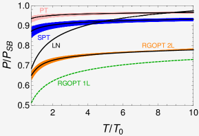
Figure 6: $P/P_{SB}(T/T_{0})$ in high-$T$ approximation for $N=4$, $g(M_{0}=2\pi T_{0})=1$, and scale variation $1/2<\alpha<2$. Pink range: PT; blue range: SPT; black: LN; orange range: two-loop RGOPT; green dashed line: one-loop RGOPT.

VI.5 Comparison with next-to-leading $1/N$ expansion

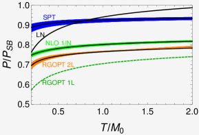
Figure 7: $P/P_{\rm SB}(T/M_{0})$ in high-$T$ approximation for $N=4$, $g(M_{0})=1=g_{LN}(M_{0})/2$ and scale variation $1/2<\alpha<2$. Same captions as in Fig. 6, with added comparison to $1/N$ NLO pressure (green range).

Next, since the RGOPT incorporates finite $N$, it is of interest to also compare our results with the ones obtained from the nonperturbative $1/N$ expansion at NLO warringa . Since the $1/N$ NLO exact solution in Ref. warringa is rather involved, to make the comparison simpler we consider the $1/N$ NLO pressure in the high-$T$ approximation only. It reads warringa

$$P_{1/Nnlo}\approx T^{2}\frac{\pi}{6}(N-1)-\frac{T}{4}(N-2)m_{1/Nnlo},$$ (75)

where

$$m_{1/Nnlo} \approx T\pi\left[\left(\frac{2\pi}{g_{LN}}-\frac{\ln 4}{N}\right)\left(1+\frac{2}{N}\right)\right.$$ (76)

$$- \left.\gamma_{E}-\ln\left(\frac{M}{4\pi T}\right)\right]^{-1},$$

where the (rescaled) coupling has the same meaning as the LN one, Eq. (46). First, notice that already the one-loop RGOPT mass gap, Eq. (60), upon expanding it in $1/N$, has a quite similar expression as (76), only missing the $\ln 4/N$ term. In Fig. 7 we show the pressure, all evaluated in the high-$T$ limit and obtained with the different approximations, with the scale dependence illustrated as previously, for $1/2<\alpha<2$. It clearly displays how, from one to two-loop, the RGOPT pressure appears to converge rather well to the NLO $1/N$ result. Note also that the nonperturbative NLO $1/N$ pressure exhibits a residual, though moderate, scale dependence: this comes from the fact that the exact NLO $1/N$ running coupling warringa , which is given by Eq. (43) upon rescaling the coupling from Eq. (46), does not perfectly match the scale dependence of Eq. (76). This is analogous to the origin of the residual scale dependence of the two-loop RGOPT pressure, already explained above, which indeed appears in Fig. 7 to be of a similar range as the NLO $1/N$ scale dependence.

VI.6 Further improving residual scale dependence

We have previously explained why, despite the explicit perturbatively RG invariant RGOPT construction, there is a moderate residual scale dependence within the two-loop results. Now, given that we restricted our analysis at the two-loop order, one may wonder generally if it is possible to further improve the RGOPT scale invariance at this order. As mentioned in the introductory part of Sec. V, if we could obtain a simultaneous solution of both Eqs. (48) and (51), therefore getting rid of using the perturbative (massless) running from Eq. (55), we could intuitively expect a further reduced, minimal scale dependence (but still not expecting perfect scale invariance at a given finite order of the RGOPT modified expansion, which obviously remains as an approximation to the truly nonperturbative result). But since in the NLSM such nontrivial solution does not exist at two-loop order, an interesting question that we address now is whether the scale dependence may be further improved nevertheless, by using some alternative procedure.

In fact it is only the combination of the exact two-loop mass optimization prescription (MOP) Eq. (48) with the exact RG Eq. (51), which leads to the trivial solution $g=0$, Eq. (53). Now, since RGOPT is still a perturbatively constructed approximation, it is perhaps too contrived to require such exact solutions at two-loop order. Thus, one possible trick is to bypass the actual triviality of the combined solution by simply approximating one of the two equations. Typically, the simplest procedure is to keep the RG Eq. (51) as exact, giving the mass gap $m(g(T))$ just as previously, while considering the other exact physical solution of Eq. (48), given by Eq. (41), as defining an effective temperature-dependent coupling $g(T)$, but approximating the latter by truncating the thermal mass to its purely perturbative first order high-$T$ expression, Eq. (61). This gives the result

$$b_{0}\,g_{eff}(m,M)=\left[\ln\frac{M}{m}-2J_{1}(\frac{m}{T})\right]^{-1}$$

$$\simeq\left\{\ln\left[\frac{2M}{(N-2)g\,T}\right]-2J_{1}(\frac{(N-2)g}{2})\right\}^{-1}.$$ (77)

There is one minor subtlety at this stage: while the standard perturbative running, e.g., Eq. (43) at one-loop order, is calibrated such that the central value $\alpha=1$ corresponds exactly to $M=2\pi T$, this has no reason to be the case for the running coupling (77), having a more nonperturbative dependence. Thus, to get a sensible comparison of scale dependence, namely for identical central coupling values $g(M_{0})$, we have to match $M_{0}$ such that $g_{eff}(M=\alpha M_{0})\equiv g(M_{0})$ for $\alpha=1$, which is obtained for an appropriate central value $\alpha$ upon setting $M\equiv 2\pi\alpha$ in Eq. (77). More precisely, for $g(M_{0})=1$ this matching happens for $\alpha\simeq 2e^{-\gamma_{E}}/2\simeq 1.12$, a very moderate shift of renormalization scale calibration.

Now, by combining the approximate solution Eq. (77) with the Eq. (51), we do obtain a nontrivial coupled $\{\bar{g},\bar{m}\}$ solution, and Eq. (77) has sound properties of an effective coupling, being consistent (at least at one-loop order) with the standard running coupling (43). Morever, we stress that Eq. (77) is not put by hand, but it is a direct consequence of Eq. (41), at a minimal extra work cost, since one already knows all the ingredients from the above calculations at this stage. Using Eq. (77), one can examine the resulting scale dependence that follows from this alternative procedure. This is illustrated for the pressure, as compared with the previous results using the purely perturbative running (55), in Fig. 8. One observes a definite further improvement, by a factor two roughly, specially in the intermediate $T/M_{0}$ zoomed in region, where the previous scale dependence was the largest.

Figure 8: $P/P_{SB}$ (zoomed in Fig. 5) for the two-loop RGOPT pressure, comparing using the perturbative two-loop running coupling Eq. (55), or the truncated RG optimized running coupling Eq. (77). For the latter, for $T/M_{0}\gtrsim 0.17$ the lower border of the range corresponds to the lower scale choice $\alpha=0.5$, and the upper border corresponds to the higher scale choice $\alpha=2$. While for $T/M_{0}\lesssim 0.17$ it is the opposite.

We have tried to pursue this construction by truncating the RGOPT thermal mass $m$ at the next two-loop order, but the scale dependence does not further improve, rather worsening. This “incompressible”, minimal residual scale dependence beyond one-loop order is actually expected from general perturbative arguments, since one cannot expect to have exact scale invariance at two-loop order or beyond. Note, moreover, that if one would push farther such approximations of Eq. (41), including more and more perturbative terms in the thermal mass expansion, one would progressively see the combined solution unavoidably reach the exact trivial one, Eq. (53), $g_{eff}\to 0$. Therefore, Eq. (77) appears to be a relatively simple and optimal effective prescription to minimize the scale dependence. Remark also that Eq. (77) has essentially a one-loop running form, when comparing with Eq. (43), but the arbitrary $T$-dependence that it involves allows to consider a more nonperturbative coupling $g$ regime, as we will illustrate next, when comparing with lattice results.

Now, as we have already emphasized before, since at two-loop RGOPT order the correct AF branch mass gap solution behaves perturbatively essentially like the one-loop solution, Eq. (41), it is not too suprising that Eq. (77) appears as an optimal running. But we must emphasize that this feature is very peculiar to the NLSM model at two-loop order, as already explained previously, with the factorized form of the two-loop mass gap solution (48) due to the specific renormalization properties of the NLSM vacuum energy. More generally for other models, the running coupling at a $n$-loop order should be optimal for the RGOPT at $n$-loop order.

VI.7 Comparison with lattice simulations

We will now compare the RGOPT results with lattice simulation ones. Apart from the early work in lattice_early , to the best of our knowledge the only available lattice thermodynamics simulation of the NLSM is the one of Ref. giacosa , which was performed for $N=3$ . To complete this comparison, we need a priori to fix an appropriate coupling value at some scale $M_{0}$, recalling that the simulation in Ref. giacosa was performed at relatively strong lattice coupling values. As required in lattice simulations, the authors consider a sequence of different (bare) lattice couplings for different $T/M_{0}$ ranges, in order to best control the approach to the continuum. Our analytical result is evidently aimed for fixing a $g(M_{0})$ input choice (its running with the scale being determined from RG properties). Moreover the RGOPT approximation effective coupling, in the $\overline{\rm MS}$ scheme, has no reasons to coincide with the lattice coupling definition. As already explained above, the combined two-loop solution for the RG Eq. (51) and the MOP Eq. (48), if it would exist at two-loop order, would determine besides the optimal mass similarly an optimal $T$-dependent coupling $\bar{g}(M,T)$, thus giving a compelling choice for comparing with lattice results. In absence of such optimal two-loop coupling for the NLSM two-loop results, there is, however, one other remarkable coupling value $g(M_{0})$ (at two-loop order), namely such that $\ln\bar{m}(0)/M_{0}=0$ exactly (i.e. such that the zero-temperature mass gap coincides with the scale $M_{0}$, with no further corrections). This happens for $g(M_{0})=2\pi$ (a value coincidentally analogous to the one obtained in the GN model JLGN for the exact optimal coupling). It thus appears to be a sensible input choice to compare with lattice, as it is also in the nonperturbative regime. In Fig. 9 we thus compare the one- and two-loop RGOPT and the LN pressure for $g(M_{0})=2\pi$ with the lattice data for $N=3$, as function of the temperature, now normalized by the $T=0$ mass gap $\bar{m}(0)$, consistently with the lattice results normalizationgiacosa .
Our LN pressure exactly coincides analytically and numerically with the one in Ref. giacosa ). The one-loop RGOPT and LN pressure are exactly scale independent for any $g$, as already pointed out before (remarking again that the only difference between one-loop RGOPT and LN is the $N-1\to N$ overall factor). It is also worth noting that, once expressed as $P(T/\bar{m}(0))$, both the one-loop RGOPT and LN pressures are actually independent of the input coupling value $g(M_{0})$: the reason for this is that the one-loop pressure Eq. (44) (and therefore also its large-$N$ limit) do not depend explicitly on $g$, while the $g(M)$ dependence is entirely absorbed within $\bar{m}(0)$ from the mass gap Eq. (41). (Accordingly the one-loop and LN pressures in Fig 9 do not get closer nor farther from the lattice data for other $g(M_{0})$ choices).
But this remarkable feature holds only approximately at two-loop order, due to the no longer matched $g(M)$-dependence between the pressure Eq. (39) and the two-loop mass gap equation. Moreover this mismatch is strongly enhanced in the peculiar $N=3$ limit in the NLSM, due to the vanishing of the two-loop $g$-dependence in the pressure Eq. (39). Consequently, for $N=3$ the two-loop RGOPT pressure happens to be accidentally much sensitive to the $g(M_{0})$ input choice. An additional drawback is that for such large reference coupling $g(M_{0})\sim 2\pi$, the unavoidable residual two-loop RGOPT scale dependence, which had remained very moderate for $g(M_{0})\lesssim 2$, is now substantially enhanced. We thus use the further improved alternative running coupling, determined by Eq. (77), but the residual scale variation appears quite sizable. Nevertheless, when we compare the RGOPT results with the scale dependence of other approximations, such as the PT or SPT for $N\neq 3$ (which for such large coupling values is well beyond any reasonable variation), the much better performance of the RGOPT is quite visible. (Remark that we do not illustrate PT and SPT here for $N=3$, since at two-loop order the SPT mass gap solution (67) trivially vanishes for $N=3$, consequently giving in Eq. (69), (72) a trivial (constant) pressure equal to the SB limit for any temperature).
Within this sizeable scale variation uncertainty, the two-loop RGOPT pressure shows a reasonably good agreement with lattice results for $T\gtrsim\bar{m}(0)$, but not so good, at least for the central renormalization scale, for low $0.2\lesssim T/\bar{m}(0)\lesssim 1$ values. However, due to the above explained important sensitivity of the two-loop pressure to the input coupling for $N=3$, the value $g(M_{0})=2\pi$ has to be considered more a reasonably good ’fit’ of the lattice data from the two-loop results, coincidentally, than a genuine prediction of RGOPT. It is intriguing that this value has other independent motivations, but it is probably more correct to conclude that this reasonable agreement is largely coincidental.

Another rather stricking result is the extremely good agreement of lattice data with LN for small to moderate $T/m(0)\lesssim 1$. While for very large $T$ values the lattice (and also the two-loop RGOPT) pressures are consistent with the true SB limit of the model Eq. (58), $P_{SB}\sim(N-1)$. This visible difference between the low- and high-$T$ regimes of the NLSM model is an important nonperturbative crosscheck: at sufficiently low $T$, nonperturbative results should reflect the unbroken $O(N)$ with actually $N$ degrees of freedom. In the RGOPT framework, similarly to the LN approximation, as we have explained the constant vacuum energy piece $m^{2}/g$ (footprint of a $\sigma$ field term), plays a crucial role in obtaining a mass gap with these expected features of the low-$T$ nonperturbative NLSM properties. While at asymptotically high-$T$ one reaches the free theory $g\to 0$ limit of the NLSM model, thus describing a gas of $N-1$ non-interacting pions, while the non-kinetic $m^{2}/g$ contribution becomes negligible. The RGOPT two-loop results roughly exhibit this overall nonperturbative behavior from low- to high-$T$ regime (although not perfectly at very low temperatures).

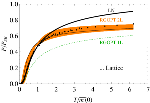
Figure 9: $P/P_{\rm SB}$ as a function of the temperature $T$ (normalized by the $T=0$ mass gap $\bar{m}(0)$) for $N=3$: LN, one- and two-loop RGOPT for $g(M_{0})=g_{LN}(M_{0})=2\pi$ and scale variation $1/2\leq\alpha\leq 2$, when using RG optimized running given by Eq. (77), compared with lattice simulations (taken from Ref. giacosa ). NB lattice data have been conveniently rescaled on vertical axis from $P/T^{2}$ in Ref giacosa to $P/P_{SB}$ (i.e., for $N=3$ this corresponds to a scaling factor of $\pi/3$).

VI.8 The Trace anomaly

It is also of interest to investigate the behavior of some other thermodynamical quantities evaluated in the RGOPT scheme and how they compare with the same quantities evaluated in the SPT and LN approximations. For example, the interaction measure $\Delta=({\cal E}-P)/T^{2}\equiv T\partial_{T}[P(T)/T^{2}]$, which is the trace of the energy-momentum tensor normalized by $T^{2}$. The interaction measure can be readily obtained from the pressure by using the definitions for the entropy density,

$$S=\frac{d}{d\,T}P(\bar{m}(g,T,M),T,M),$$ (78)

and for the energy density, ${\cal E}=-P+S\,T$.

One subtlety rooted in the optimized perturbation, is that one should evaluate the entropy according to Eq. (78), namely only after the mass gap $\bar{m}(g,T)$, which is explicitly $T$-dependent, had been replaced within the pressure expression, which, thus, becomes only a function of $g(T/M),T/M$. While the partial derivative calculated for fixed (arbitrary) $m$, ignoring the mass gap (which would give the correct result for the truly massive theory), is generally different and would lead to physically inconsistent results in the present case. Actually, at the one-loop RGOPT order, since the mass gap is defined by the constraint given by (34) and that results in Eq. (41), the two expressions coincide. This here is simply because in $dP(m(T),T)/dT=\partial P/\partial T+(\partial m/\partial T)(\partial P/\partial m)$ the last term vanishes by definition due to Eq. (34). While for the two-loop RGOPT, our mass gap prescription that guarantees real solutions is given by the RG Eq. (54), which is obviously not equivalent to Eq. (34). Likewise, the SPT mass gap, since it can only be real-defined at this order as the Debye mass (67), is also very different from the optimized mass (34). At the one-loop RGOPT order, we easily obtain simple compact analytical expressions for the entropy and trace anomaly, given, respectively, by

$$S^{\rm RGOPT}_{1L}=-T\frac{(N-1)}{\pi}\left[2J_{0}(\bar{x})+\bar{x}^{2}J_{1}(\bar{x})\right],$$ (79)

and

$$\Delta^{\rm RGOPT}_{1L}(T)-\Delta(0)=\frac{(N-1)}{4\pi}\left[\bar{x}^{2}(T)-\bar{x}^{2}(0)\right],$$ (80)

where it is understood that $\bar{x}\equiv\bar{m}(T)/T$ is given by the solution of Eq. (41) . Note that we normalize $\Delta$ by subtracting its $T=0$ expression, consistently with the pressure normalization, $\Delta(0)\equiv-2P(0)/T^{2}=(N-1)\bar{m}^{2}(0)/(4\pi T^{2})$. The corresponding LN expressions are very similar to Eq. (79) and (80), being obtained by the appropriate LN rescaling (46) and overall $N-1\to N$ usual changing.

The two-loop SPT interaction measure has also a relatively simple expression, due to the SPT mass gap being the perturbative pole mass (67) at this order, with $T$-dependence such that $\bar{m}^{\prime}_{spt}(T)=m_{spt}/T(1-b_{0}g+{\cal O}(g^{2}))$. (note also that $\Delta_{spt}(T=0)$ trivially vanishes). We obtain

$$\Delta^{\rm SPT}_{2L}(T)=\frac{g\,(N-1)}{16\pi^{2}}\bar{x}^{2}\left[4\pi b_{0}(1+2\bar{x}^{2}J_{2}(\bar{x}))\right.$$

$$\left.-(N-3)\left\{1-b_{0}g(1+2\bar{x}^{2}J_{2}(\bar{x})+\frac{3}{2}Y)\right\}Y\right],$$ (81)

where $\bar{x}_{spt}=\pi\gamma_{0}\,g(T)$ from (67) and $Y$ was defined in Eq. (49). Thus its main feature is that Eq. (81) is substantially smaller, at high and moderate $T$ values, relative to e.g. (80), being suppressed by the small SPT mass gap $\sim x^{2}_{spt}$, and has an essentially monotonic dependence on $T$.
As concerns the two-loop RGOPT, the exact analytical expressions of $S$ and $\Delta$ are rather involved and not very telling, due to the more involved nonperturbative mass gap $\bar{m}(g,T)$ expression, which we recall is obtained by solving Eq. (54). Thus, we refrain ourselves from writing down explicitly its full expression and we will only present its corresponding numerical result. As we will illustrate, however, its shape as function of $T/M$ is to a good approximation roughly similar to the simple one-loop RGOPT in (80).

In Fig. 10 we show the dependence of the interaction measure as a function of the temperature in the one- and two-loop RGOPT, two-loop SPT, and LN cases, for the same choice of $N=4$ and $g=1=g_{LN}/2$, as in the previous pressure plots shown in Figs. 2-5.

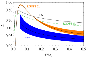
Figure 10: The interaction measure $\Delta$ as a function of the temperature $T$ (normalized by $M_{0}$) for $N=4$ and $g(M_{0})=1=g_{LN}(M_{0})/2$, with scale variation $0.5\leq\alpha\leq 2$, using the standard two-loop running coupling given by Eq. 55). Within the two-loop RGOPT and SPT, the shaded bands have the lower edge for $\alpha=0.5$ and the upper edge for $\alpha=2$. The thin line inside the shaded bands is for $\alpha=1$. (Logarithmic scale is used).

We notice from the RGOPT results shown in Fig. 10 how the inflection before the peak of $\Delta$ occurs approximately at the temperature value where $m(T)$ bends (see Fig. 4), which is an interesting feature if one recalls that in QCD the inflection occurs at $T_{c}$. It is worth to trace more precisely the origin of the peak of the RGOPT interaction measures. First, note that $\bar{x}^{2}(T/M_{0})=\bar{m}^{2}(T/M_{0})/T^{2}$, as determined from Eq. (41), is monotonically decreasing. Thus the peak only originates from its interplay with the subtracted zero-temperature reduced (squared) mass gap $\bar{x}^{2}(0)\equiv\bar{m}^{2}(0)/T^{2}$ in Eq. (80). It is easy to take the derivative with respect to $T$ of (80), upon having first determined, from Eq. (41), that

$$\bar{m}^{\prime}(T)=2\bar{x}^{3}\frac{J_{2}(\bar{x})}{1+2\bar{x}^{2}J_{2}(\bar{x})},$$ (82)

to trace analytically that (80) has an inflection point, and then a maximum at a given $t_{m}\equiv T_{m}/M_{0}$ value, determined from the solution of

$$\bar{x}^{2}(0)\equiv\frac{e^{-\frac{2}{b_{0}\,g}}}{t_{m}^{2}}=\frac{\bar{x}^{2}(t_{m})}{1+2\bar{x}^{2}(t_{m})\,J_{2}(\bar{x}(t_{m}))}.$$ (83)

For $N=4$, $g(M_{0})=1$, it gives $t_{m}\simeq 0.029$, $\bar{x}(t_{m})\simeq 1.95$, which corresponds exactly to the peak position in Fig. 10. (Note that the peak position is the same for the LN trace anomaly, for this choice of couplings). One also easily derive the peak value as

$$\Delta^{\rm RGOPT}_{1L}(t_{m})-\Delta(0) = \frac{(N-1)}{2\pi}\frac{e^{-\frac{2}{b_{0}\,g}}}{t_{m}^{2}}\bar{x}^{2}(t_{m})$$ (84)

$$\times J_{2}(\bar{x}(t_{m}))$$

which gives $\simeq 0.38$, like is seen in Fig. 10. For the two-loop RGOPT interaction measure, it is more difficult to trace analytically but this quantity follows similar features, except that the bending of $\bar{m}$ is delayed to larger $T/M_{0}$ (see again Fig. 4), so are the corresponding inflection point, and subsequent peak in Fig. 10. Thus, although there is no phase transition in two dimensions, the trace anomaly has a nontrivial structure with an inflection point followed by a peak, due to the occurence of a mass gap, signaling the breakdown of scale invariance already at $T=0$, and the nontrivial $T$-dependence of this mass gap: since $\bar{m}(0)$ in Eq. (42) reflects dimensional transmutation, (80) (or similarly its two-loop generalization) involve nonperturbative power contributions. Note also that the RGOPT prediction is that ${\cal E}-P\equiv\Delta\,T^{2}$ grows quadratically with $T$ at high temperatures, up to $\ln T$ terms, as easily established from the high-$T$ expression of (80) using $\bar{x}(T)$ from Eq. (60): $\Delta(T\gg M_{0})\simeq 1/\ln(T/M_{0})$. This behavior may be viewed as the two-dimensional analog, and qualitatively compared with four-dimensional Yang-Mills theory where a quadratic behavior has been found in the LQCD evaluations performed in Ref. karsch_glue , and analytically supported by convincing arguments in quadraticDelta ; RArriola .

Another interesting feature shown by the results in Fig. 10 is that the two-loop RGOPT predicts that after the “transition” (inflection) the system interacts in a much stronger way than predicted by the LN and the one-loop RGOPT, which have smaller thermal masses (see Fig. 3). In this respect, it is again instructive to compare our results for the interaction measure, given by Fig. 10, with those obtained in Ref. HTLPT3loop and shown in Fig. 12 in that reference. While the leading-order (LO) and next-to-leading order (NLO) HTLpt results show an essentially perturbative behavior, the three-loop (NNLO) HTLpt interaction measure is closer to the LQCD simulations karsch_glue ; karschQCD (although not reproducing the lattice data peak). From this comparison one can appreciate that the two-loop RGOPT interaction measure has a shape similar to the one obtained in the LQCD simulations. In contrast the two-loop SPT interaction measure looks qualitatively more similar to the three-loop HTLpt results HTLPT3loop , which we understand as originating from the accessible exact low $T$ dependence in the NLSM case. It is a monotonic function of $T$ with no peak at any $T/M_{0}$ (as we also checked from Eq. (81) and going further below the $T/M_{0}$ values shown in Fig. 10).

VII Conclusions

We have applied the recently developed RGOPT nonperturbative framework to investigate thermodynamical properties of the asymptotically free $O(N)$ NLSM in two dimensions, and illustrate results for $N=3$ and $N=4$. Our application shows how simple perturbative results can acquire a robust nonperturbative predictive power by combining renormalization group properties with a variational criterion used to fix the (arbitrary) “quasi-particle” RGOPT mass.

In particular, a non-trivial scale invariant result was obtained by considering the lowest order contribution to the pressure, which represents a remarkable result if one considers that the whole large-$N$ series can be readily reproduced upon taking the $N\to\infty$ limit within the RGOPT. In addition, at realistic finite $N$ values and high temperatures, the lowest order RGOPT pressure converges to the correct Stefan-Boltzmann limit, while the LN result overshoots it. Next, in accordance with other previous finite temperature applications jlprd ; jlprl , the NLO (two-loop) order RGOPT results display a very mild residual scale dependence when compared to the standard SPT/OPT results. The much reduced residual scale dependence is due to the explicitly RG invariant construction at all stages, as we recall: first from retaining (or reintroducing, if absent) appropriate finite vacuum energy subtraction, Eq. (30), to restore perturbative RG invariance of the vacuum energy of the model. Second, by maintaining RG invariance while modifying the perturbative series with a generalized RG-dictated interpolation, Eq. (33) with (37). In contrast in related variational SPT or HTLpt approaches, the vacuum energy subtraction are omitted, and the simpler linear interpolation is used. One should remark however that in thermal theories, the omission of additional vacuum energy term is essentially innocuous at lowest order, since the thermal mass $m_{T}$ has itself a perturbative origin: here for the two-dimensional NLSM, $m_{T}\sim gT+{\cal O}(g^{2})$, (see Eq. (67)), such that, if uncancelled, the remnant term (29) is formally of higher ${\cal O}(g^{2})$ order. These features are completely similar in four-dimensional models jlprd , where the vacuum energy involves $m^{4}$ terms, while the thermal mass behaves for small $g$ as $m^{2}_{T}\sim gT$. Therefore the SPT or HTLpt formal lack of scale invariance at one-loop order is essentially “screened” by thermal masses, at least as long as $g$ takes perturbative values. But conversely it essentially explains why a more dramatic scale dependence is seen to resurface at higher orders, in particular at three-loop order in resummed HTLpt HTLPT3loop .

We also obtain a reasonable agreement of the RGOPT pressure with known lattice results for $N=3$, in the full temperature range, with the expected nonperturbative behavior of the NLSM from low- to high-$T$ regime (but the agreement with lattice results is not quite good at low temperature). However, this agreement is largely accidental at two-loops, coincidentally for a somewhat large input coupling choice $g(M_{0})\simeq 2\pi$. We remark that these rather odd properties of the two-loop NLSM RGOPT results essentially originate from the perturbative two-loop pressure contribution vanishing for $N=3$, see Eq. (39), therefore inducing a severe mismatch in the good scale invariance properties otherwise verified for any other $N>3$. We can speculate an a priori much better behavior at three-loops for $N=3$, having simply determined from lower orders, using solely RG invariance properties, that the three-loop pressure contribution does not vanish for $N=3$, but a more precise investigation is well beyond our present scope.

The NLSM thermodynamical observables obtained from two-loop RGOPT display a physical behavior that is more in line with LQCD predictions for pure Yang-Mills four-dimensional theories, as compared with the two-loop order SPT. Perhaps the most striking result, also in view of applications to QCD, is that the one- and two-loop RGOPT interaction measure $\Delta$ exhibit some characteristic nonperturbative features somewhat similar to the QCD interaction measure. Although as previously explained the underlying physics is very different since in two dimensions there is no phase transition, and the inflection and peak in the NLSM interaction measure reflect simply the broken scale invariance from a mass gap. Yet the underlying mechanism appears here simpler but somewhat similar to the one advocated for QCD quadraticDelta ; RArriola ; giacosaDelta , in the sense that this peak originates from an interplay between thermal perturbative and nonperturbative $T=0$ (power) contributions, present in RGOPT results. One may qualitatively compare these features with the HTLpt interaction measure, which is much closer to the lattice QCD results at three-loops HTLPT3loop , but does not show a transition peak. While this is made possible in the present NLSM case due to the rather simple structure of the model, giving an analytical handle to the full temperature dependence up to two-loop order. Apart from such possible technical limitations for a similar application to thermal QCD, the present NLSM results nevertheless confirm that the recently proposed RGOPT approach stands as a robust analytical tool to treat renormalizable theories at extreme conditions.

Finally it would be of much interest to compare our NLSM thermodynamical results with other lattice simulation results for other $N$ values, but unfortunately to our knowledge no such simulations at finite temperature are available up to now for $N>3$.

References

- (1) J. P. Blaizot, E. Iancu and A. Rebhan, “Thermodynamics of the high temperature quark gluon plasma,” In *Hwa, R.C. (ed.) et al.: Quark gluon plasma* 60-122 [hep-ph/0303185]; U. Kraemmer and A. Rebhan, “Advances in perturbative thermal field theory,” Rept. Prog. Phys. 67, 351 (2004).
- (2) Y. Aoki, G. Endrodi, Z. Fodor, S. D. Katz and K. K. Szabo, “The Order of the quantum chromodynamics transition predicted by the standard model of particle physics,” Nature 443, 675 (2006); Y. Aoki, Z. Fodor, S. D. Katz and K. K. Szabo, “The QCD transition temperature: Results with physical masses in the continuum limit,” Phys. Lett. B 643, 46 (2006); M. Cheng et al., “The Transition temperature in QCD,” Phys. Rev. D 74, 054507 (2006).
- (3) M. Cheng et al., “The QCD equation of state with almost physical quark masses,” Phys. Rev. D 77, 014511 (2008).
- (4) V.I. Yukalov, “Model of a hybrid crystal,” Theor. Math. Phys. 28, 652 (1976); W. E. Caswell, “Accurate Energy Levels for the Anharmonic Oscillator and a Summable Series for the Double Well Potential in Perturbation Theory,” Annals Phys. 123, 153 (1979); I. G. Halliday and P. Suranyi, “Convergent Perturbation Series for the Anharmonic Oscillator,” Phys. Lett. 85B, 421 (1979); R. P. Feynman and H. Kleinert, “Effective Classical Partition Functions,” Phys. Rev. A 34, 5080 (1986); H. F. Jones and M. Moshe, “Renormalization of the Linear Delta Expansion: The Gross-Neveu Model,” Phys. Lett. B 234, 492 (1990); A. Neveu, “Variational improvement of perturbation theory and/or perturbative improvement of variational calculations,” Nucl. Phys. Proc. Suppl. 18B, 242 (1991); V. I. Yukalov, “Method of self‐similar approximations,” J. Math. Phys (N.Y) 32, 1235 (1991); C. M. Bender, F. Cooper, K. A. Milton, M. Moshe, S. S. Pinsky and L. M. Simmons, Jr., “Delta expansion for local gauge theories. 1. A One-dimensional model,” Phys. Rev. D 45, 1248 (1992); H. Yamada, “Spontaneous symmetry breaking in QCD,” Z. Phys. C 59, 67 (1993); doi:10.1007/BF01555840 A. N. Sisakian, I. L. Solovtsov and O. P. Solovtsova, “beta function for the phi**4 model in variational perturbation theory,” Phys. Lett. B 321, 381 (1994). H. Kleinert, “Strong coupling phi**4 theory in four epsilon dimensions, and critical exponents,” Phys. Rev. D 57, 2264 (1998); Addendum: [Phys. Rev. D 58, 107702 (1998)]. H. Kleinert, “Strong coupling phi**4 theory in four epsilon-dimensions, and critical exponents,” Phys. Lett. B 434, 74 (1998).
- (5) P. M. Stevenson, “Optimized Perturbation Theory,” Phys. Rev. D 23, 2916 (1981).
- (6) S. Chiku and T. Hatsuda, “Optimized perturbation theory at finite temperature,” Phys. Rev. D 58, 076001 (1998).
- (7) F. Karsch, A. Patkos and P. Petreczky, “Screened perturbation theory,” Phys. Lett. B 401, 69 (1997).
- (8) J. O. Andersen, E. Braaten and M. Strickland, “Screened perturbation theory to three loops,” Phys. Rev. D 63, 105008 (2001); J. O. Andersen and M. Strickland, “Mass expansions of screened perturbation theory,” Phys. Rev. D 64, 105012 (2001); J. O. Andersen and M. Strickland, “Resummation in hot field theories,” Annals Phys. 317, 281 (2005).
- (9) H. Kleinert, “Five-Loop Critical Temperature Shift in Weakly Interacting Homogeneous Bose–Einstein Condensate,” Mod. Phys. Lett. B 17, 1011 (2003); B. M. Kastening, “Bose-Einstein condensation temperature of homogenous weakly interacting Bose gas in variational perturbation theory through six loops,” Phys. Rev. A 68, 061601 (2003); B. M. Kastening, “Bose-Einstein condensation temperature of homogenous weakly interacting Bose gas in variational perturbation theory through seven loops,” Phys. Rev. A 69, 043613 (2004).
- (10) J. L. Kneur, A. Neveu and M. B. Pinto, “Improved optimization of perturbation theory: Applications to the oscillator energy levels and Bose-Einstein condensate critical temperature,” Phys. Rev. A 69, 053624 (2004); J. L. Kneur, M. B. Pinto and R. O. Ramos, “Convergent resummed linear delta expansion in the critical (3-d) model,” Phys. Rev. Lett. 89, 210403 (2002).
- (11) H. Caldas, J.-L. Kneur, M. B. Pinto and R. O. Ramos, “Critical dopant concentration in polyacetylene and phase diagram from a continuous four-Fermi model,” Phys. Rev. B 77, 205109 (2008).
- (12) J. L. Kneur, M. B. Pinto, R. O. Ramos and E. Staudt, “Emergence of tricritical point and liquid-gas phase in the massless 2+1 dimensional Gross-Neveu model,” Phys. Rev. D 76, 045020 (2007); J. L. Kneur, M. B. Pinto, R. O. Ramos and E. Staudt, “Updating the phase diagram of the Gross-Neveu model in 2+1 dimensions,” Phys. Lett. B 657, 136 (2007); J. L. Kneur, M. B. Pinto and R. O. Ramos, “Phase diagram of the magnetized planar Gross-Neveu model beyond the large-N approximation,” Phys. Rev. D 88, 045005 (2013).
- (13) M. B. Pinto and R. O. Ramos, “High temperature resummation in the linear delta expansion,” Phys. Rev. D 60, 105005 (1999); M. B. Pinto and R. O. Ramos, “A Nonperturbative study of inverse symmetry breaking at high temperatures,” Phys. Rev. D 61, 125016 (2000); R. L. S. Farias, G. Krein and R. O. Ramos, “Applicability of the linear expansion for the field theory at finite temperature in the symmetric and broken phases,” Phys. Rev. D 78, 065046 (2008); D. C. Duarte, R. L. S. Farias and R. O. Ramos, “Optimized perturbation theory for charged scalar fields at finite temperature and in an external magnetic field”, Phys. Rev. D 84, 083525 (2011).
- (14) T. E. Restrepo, J. C. Macias, M. B. Pinto and G. N. Ferrari, “Dynamical Generation of a Repulsive Vector Contribution to the Quark Pressure,” Phys. Rev. D 91, 065017 (2015).
- (15) J. L. Kneur, M. B. Pinto and R. O. Ramos, “Thermodynamics and Phase Structure of the Two-Flavor Nambu–Jona-Lasinio Model Beyond Large-,” Phys. Rev. C 81, 065205 (2010); J. L. Kneur, M. B. Pinto, R. O. Ramos and E. Staudt, “Vector-like contributions from Optimized Perturbation in the Abelian Nambu–Jona-Lasinio model for cold and dense quark matter,” Int. J. Mod. Phys. E 21, 1250017 (2012); D. C. Duarte, R. L. S. Farias, P. H. A. Manso and R. O. Ramos, “Optimized perturbation theory applied to the study of the thermodynamics and BEC-BCS crossover in the three-color Nambu–Jona-Lasinio model,” Phys. Rev. D 96, 056009 (2017).
- (16) E. Braaten and R. D. Pisarski, “Soft Amplitudes in Hot Gauge Theories: A General Analysis,” Nucl. Phys. B 337, 569 (1990).
- (17) J. O. Andersen, E. Braaten and M. Strickland, “Hard thermal loop resummation of the free energy of a hot gluon plasma,” Phys. Rev. Lett. 83, 2139 (1999); J. O. Andersen, E. Braaten and M. Strickland, “Hard thermal loop resummation of the free energy of a hot quark - gluon plasma,” Phys. Rev. D 61, 074016 (2000).
- (18) J. O. Andersen, M. Strickland and N. Su, “Gluon Thermodynamics at Intermediate Coupling,” Phys. Rev. Lett. 104, 122003 (2010); “Three-loop HTL gluon thermodynamics at intermediate coupling,” JHEP 1008, 113 (2010); J. O. Andersen, L. E. Leganger, M. Strickland and N. Su, “Three-loop HTL QCD thermodynamics,” JHEP 1108, 053 (2011).
- (19) S. Mogliacci, J. O. Andersen, M. Strickland, N. Su and A. Vuorinen, “Equation of State of hot and dense QCD: Resummed perturbation theory confronts lattice data,” JHEP 1312, 055 (2013); N. Haque, J. O. Andersen, M. G. Mustafa, M. Strickland and N. Su, “Three-loop pressure and susceptibility at finite temperature and density from hard-thermal-loop perturbation theory,” Phys. Rev. D 89, 061701 (2014); N. Haque, A. Bandyopadhyay, J. O. Andersen, M. G. Mustafa, M. Strickland and N. Su, “Three-loop HTLpt thermodynamics at finite temperature and chemical potential,” JHEP 1405, 027 (2014).
- (20) J. O. Andersen, L. Kyllingstad and L. E. Leganger, “Pressure to order g**8 log g of massless phi**4 theory at weak coupling,” JHEP 0908, 066 (2009).
- (21) J.-L. Kneur and A. Neveu, “Renormalization Group Improved Optimized Perturbation Theory: Revisiting the Mass Gap of the O(2N) Gross-Neveu Model,” Phys. Rev. D 81, 125012 (2010).
- (22) J.-L. Kneur and A. Neveu, “ from Renormalization Group Optimized Perturbation,” Phys. Rev. D 85, 014005 (2012).
- (23) J. L. Kneur and A. Neveu, “ from and Renormalization Group Optimized Perturbation Theory,” Phys. Rev. D 88, 074025 (2013).
- (24) J. L. Kneur and A. Neveu, “Chiral condensate from renormalization group optimized perturbation,” Phys. Rev. D 92, 074027 (2015).
- (25) J.-L. Kneur and M. B. Pinto, “Scale Invariant Resummed Perturbation at Finite Temperatures,” Phys. Rev. Lett. 116, 031601 (2016).
- (26) J.-L. Kneur and M. B. Pinto, “Renormalization Group Optimized Perturbation Theory at Finite Temperatures,” Phys. Rev. D 92, 116008 (2015).
- (27) J. P. Blaizot, A. Ipp and N. Wschebor, “Calculation of the pressure of a hot scalar theory within the Non-Perturbative Renormalization Group,” Nucl. Phys. A 849, 165 (2011).
- (28) D. G. C. McKeon and A. Rebhan, “Renormalization group summation and the free energy of hot QCD,” Phys. Rev. D 67, 027701 (2003)
- (29) E. Megias, E. Ruiz Arriola and L. L. Salcedo, “Trace Anomaly, Thermal Power Corrections and Dimension Two condensates in the deconfined phase,” Phys. Rev. D 80, 056005 (2009).
- (30) J. O. Andersen, D. Boer and H. J. Warringa, “Thermodynamics of the O(N) nonlinear sigma model in (1+1)-dimensions,” Phys. Rev. D 69, 076006 (2004).
- (31) E. Seel, D. Smith, S. Lottini and F. Giacosa, “Thermodynamics of the O(3) model in 1+1 dimensions: lattice vs. analytical results,” JHEP 1307, 010 (2013).
- (32) E. Brezin, J. Zinn-Justin and J. C. Le Guillou, “Renormalization of the Nonlinear Sigma Model in (Two + Epsilon) Dimension,” Phys. Rev. D 14, 2615 (1976).
- (33) J. Zinn-Justin, Quantum field theory and critical phenomena (Clarendon Press, Oxford, Third Edition, 1996).
- (34) N. D. Mermin and H. Wagner, “Absence of ferromagnetism or antiferromagnetism in one-dimensional or two-dimensional isotropic Heisenberg models,” Phys. Rev. Lett. 17, 1133 (1966).
- (35) S. R. Coleman, “There are no Goldstone bosons in two-dimensions,” Commun. Math. Phys. 31, 259 (1973).
- (36) P. Hasenfratz, M. Maggiore and F. Niedermayer, “The Exact mass gap of the O(3) and O(4) nonlinear sigma models in d = 2,” Phys. Lett. B 245, 522 (1990); “The Exact mass gap of the O(N) sigma model for arbitrary in ,” Phys. Lett. B 245, 529 (1990).
- (37) H. Makino and H. Suzuki, “Renormalizability of the gradient flow in the 2D non-linear sigma model,” PTEP 2015, 033B08 (2015).
- (38) M. E. Peskin and D. V. Schroeder, An Introduction to quantum field theory (Reading, USA, Addison-Wesley, 1995)
- (39) J. I. Kapusta and C. Gale, Finite-Temperature Field Theory: Principles and Applications (Cambridge University Press, Cambridge, 2006).
- (40) M. Dine and W. Fischler, “The Thermodynamics of the Nonlinear Model: A Toy for High Temperature QCD,” Phys. Lett. 105B, 207 (1981).
- (41) S. Hikami and E. Brezin, “Three Loop Calculations in the Two-Dimensional Nonlinear Sigma Model,” J. Phys. A 11, 1141 (1978).
- (42) B. M. Kastening, “Renormalization group improvement of the effective potential in massive phi**4 theory,” Phys. Lett. B 283, 287 (1992); M. Bando, T. Kugo, N. Maekawa and H. Nakano, “Improving the effective potential,” Phys. Lett. B 301, 83 (1993); C. Ford, D. R. T. Jones, P. W. Stephenson and M. B. Einhorn, “The Effective potential and the renormalization group,” Nucl. Phys. B 395, 17 (1993).
- (43) H. Kleinert and V. I. Yukalov, “Highly accurate critical exponents from self-similar variational perturbation theory,” Phys. Rev. E 71, 026131 (2005). [cond-mat/0402163].
- (44) J. M. Cornwall, R. Jackiw and E. Tomboulis, “Effective Action for Composite Operators,” Phys. Rev. D 10, 2428 (1974).
- (45) S. K. Gandhi, H. F. Jones and M. B. Pinto, “The delta expansion in the large N limit,” Nucl. Phys. B 359, 429 (1991).
- (46) M. B. Pinto and R. O. Ramos, “High temperature resummation in the linear delta expansion,” Phys. Rev. D 60, 105005 (1999); M. B. Pinto and R. O. Ramos, ‘̀A Nonperturbative study of inverse symmetry breaking at high temperatures,” Phys. Rev. D 61, 125016 (2000)
- (47) R. L. S. Farias, G. Krein and R. O. Ramos, “Applicability of the Linear delta Expansion for the lambda phi**4 Field Theory at Finite Temperature in the Symmetric and Broken Phases,” Phys. Rev. D 78, 065046 (2008).
- (48) F. Brau and F. Buisseret, “Glueballs and statistical mechanics of the gluon plasma,” Phys. Rev. D 79, 114007 (2009).
- (49) A. Peshier, B. Kampfer, O. P. Pavlenko and G. Soff, “A Massive quasiparticle model of the SU(3) gluon plasma,” Phys. Rev. D 54, 2399 (1996).
- (50) P. Castorina and M. Mannarelli, “Effective degrees of freedom and gluon condensation in the high temperature deconfined phase,” Phys. Rev. C 75, 054901 (2007).
- (51) G. Boyd, J. Engels, F. Karsch, E. Laermann, C. Legeland, M. Lutgemeier and B. Petersson, “Thermodynamics of SU(3) lattice gauge theory,” Nucl. Phys. B 469, 419 (1996).
- (52) A. Bazavov et al. [HotQCD Collaboration], “Equation of state in ( 2+1 )-flavor QCD,” Phys. Rev. D 90, 094503 (2014);
- (53) S. Spiegel, “Thermodynamics of the two-dimensional O(3) sigma model with fixed point lattice action,” Phys. Lett. B 400, 352 (1997) doi:10.1016/S0370-2693(97)00346-8 [hep-lat/9611027].
- (54) R. D. Pisarski, “Fuzzy Bags and Wilson Lines,” Prog. Theor. Phys. Suppl. 168, 276 (2007).
- (55) F. Giacosa, “Analytical study of a gas of gluonic quasiparticles at high temperature: Effective mass, pressure and trace anomaly,” Phys. Rev. D 83, 114002 (2011).