Optimal Control Problem in a Stochastic Model
with Periodic Hits on the Boundary of a Given Subset
of the State Set (Tuning Problem)

Abstract

In this paper, a general stochastic model with controls applied at the moments when the random process hits the boundary of a given subset of the state set is proposed and studied. The general concept of the model is formulated and its possible applications in technical and economic systems are described. Two versions of the general stochastic model, the version based on the use of a continuous-time semi-Markov process with embedded absorbing Markov chain and the version based on the use of a discrete-time Markov process with absorbing states, are analyzed. New representations of the stationary cost index of the control quality are obtained for both versions. It is shown that this index can be represented as a linear-fractional integral functional of two discrete probability distributions determining the control strategy. The results obtained by the author of this paper about an extremum of such functionals were used to prove that, in both versions of the model, the optimal control is deterministic and is determined by the extremum points of functions of two discrete arguments for which the explicit analytic representations are obtained. The perspectives of the further development of this stochastic model are outlined.

Key words: stochastic models with controls, controlled stochastic processes, stochastic model with controls at the moments of hitting the state set boundary, controlled semi-Markov process, stochastic models with absorptions, stochastic tuning problem.

Introduction

The following phenomenon is observed when many processes of stochastic character encountered in technical and economic systems are analyzed. At certain times, the basic stochastic process describing the system under study can leave a given subset of states which are assumed to be admissible. The process can be returned to the subset of admissible states by an external action which can be treated as a control in the stochastic model. As a result of the control action, the process returns to one of the states in the admissible set. In this case, the state itself (or the number of this state) into which the process is taken by the external action is a control parameter or a decision. If the decision is accepted by the stochastic scheme, then it is assumed that the state into which the process is taken is determined by a certain probability distribution which can be called a controlling distribution. After the basic stochastic process is transferred to one of the admissible states, it again begins to evolve independently of the past, i.e., its behavior depends only on the state where it was taken by the external action (control). At a certain time, the basic process again leaves the set of admissible states, and then the external control action is applied according to the above-cited rules. The problem of control optimization is to find controlling probability distributions on which a certain parameter of the control efficiency attains an extremum.

The above-formulated ideas, which are based on specific characteristics of operation of actual systems, form the concept of a stochastic model with controls applied at the moments when the basic stochastic process attains the boundary of a given subset of the state set. Let us consider the possible applications of such a model in technical and economic systems in more detail.

For a technical system, a subset of admissible states can be interpreted as the set of operation states, and the output from this set means the system failure. The transition of the basic process into the subset of admissible states (external control action) is a reconstructing action applied to this system to re-establish its operation. The state of the basic process immediately after the control action determines the form of the reconstructing action, i.e., the character of the reconstruction. Thus, in applications, the problem of choosing the optimal control action in the form of optimal controlling probability distribution is the problem of determining the optimal form of reconstruction after the system failure.

The corresponding stochastic control model is also meaningful for economic systems. The basic stochastic process is assumed to describe the variations in some economic parameter (price of financial assets on the stock market, prices of a product on the goods market, currency price at currency auctions). The set of admissible states can be interpreted as the set of values of this parameter, which are favorable or acceptable for a special agent of the market applying an external control action to the corresponding financial parameter. Such a special agent of the market is usually an authorized governmental structure. The output of the basic process from a given subset of admissible states is undesirable from the standpoint of this market agent. The control action can involve different actions of the market agent aimed at changing the values of the corresponding financial parameter. A specific example of such actions is the central bank currency intervention aimed at changing the exchange rate of a currency. A similar example is the grain intervention performed by the grain fund, an authorized structure of the Ministry of Agriculture, aimed at changing the prices of different cereal crops. As a results of such actions, the process value (basic parameter) returns to the set of admissible states and the evolution of this parameter value goes on independently of the past and depends only on the new initial value formed by the external control action. The above-cited financial parameter (basic process) continues to evolve according to the laws of free market in the same economical situation as at the preceding state until it again leaves the subset of admissible states and a new control action is applied.

It follows from the above considerations that developing a stochastic model with controls at the moments of hitting the boundary of a certain subset of the state set and solving the corresponding optimal control problem is an actual problem of applied mathematics. In what follows, such a problem is called a tuning problem, which reflects the above-described external action on the basic parameter of a technical or an economic system.

In the present paper, we consider the following two possible versions of the general stochastic model discussed above. The first version (continuous time) is based on a semi-Markov stochastic process with finitely many states, which has an embedded absorbing Markov chain. The absorbing states are assumed to the boundary states, and the other states are internal and admissible. After absorption, a control action taking the process into one of the internal admissible states is applied. The further evolution of the process continues independently of the past and is described by the probability characteristics of the initial semi-Markov process until the next absorption occurs. The second version (discrete time) involves the Markov chain with two absorbing states which are assumed to be boundary states. The other states are assumed to be internal and admissible. The evolution of the discrete-time model obeys similar laws. In both versions, we pose and solve optimal control problems for stationary cost indices which, according to their economic content, are the mean specific profits. Thus, two tuning problems related to various stochastic models are solved in this paper.

1 Extremum problem for linear-fractional
integral functionals defined on a set
of discrete probability distributions

To solve the optimal control problem formulated below, we first recall a certain general result of the theory of extremum problems, namely, a theorem about an unconditional extremum for a linear-fractional integral functional on a set of probability measures. Such a theorem was formulated by the author in [1], where it was also shown that this result is a theoretical foundation for solving optimal control problems for a semi-Markov stochastic process with a finite set of states. Further, the theorem about an unconditional extremum for a linear-fractional integral functional was proved in [2] and its application to solving the optimal control problem for a semi-Markov process was justified there in detail. We note that the stochastic scheme of control at the moments of hitting the boundary of a given subset of the state set, which is proposed in this paper, is a special version of general control of a semi-Markov process, which differs from the version considered in fundamental works [3,4] and in contemporary studies (see, e.g., [5,6]). Thus, the tuning problem does not reduce to the standard control problem for a semi-Markov process, and a separate analysis is required to solve this problem. To explain such an analysis, we consider a special version of assertions about an unconditional extremum of a linear-fractional integral functional defined on a set of discrete probability distributions.

We consider a set of discrete sets $U_{i}={1,2,\dots,n_{i}}$, $i=1,2,\dots,N$, $N<\infty$. The number of elements in each set $U_{i}$ can be either finite or countable: $n_{i}\leq\infty$, $i=1,2,\dots,N$. In what follows, these sets are interpreted as sets of admissible solutions (controls) accepted in different states of the stochastic model, but in this section, they are abstract. On each set $U_{i}$, we introduce a collection of all possible probability distributions of the form $\alpha^{(i)}=(\alpha_{1}^{(i)},\alpha_{2}^{(i)},\dots,\alpha_{n_{i}}^{(i)})$, $\alpha_{s}^{(i)}\geq 0$, $s=1,2,\dots,n_{i}$; $\sum\limits_{s=1}^{n_{i}}\alpha_{s}^{(i)}=1$, $i=1,2,\dots,N$. We denote such a set of probability distributions defined on $U_{i}$ by $\Gamma_{d}^{(i)}$, $i=1,2,\dots,N$. Further, we consider the Cartesian product of spaces $U=U_{1}\times U_{2}\times\dots\times U_{N}$. Following the classical scheme of introducing the measure on a Cartesian product of spaces [7], we introduce the probability measure on $U$ as the product of probability measures on the spaces $U_{1},U_{2},\dots,U_{N}$ determined by the distributions $\alpha^{(1)},\alpha^{(2)},\dots,\alpha^{(N)}$. Thus, the probability measure on $U$ is given by the set of probability distributions $\alpha^{(1)}$, $\alpha^{(2)},\dots,\alpha^{(N)}$. We denote the set of probability measures on $U$ by $\Gamma_{d}$. Several additional conditions related to the set $\Gamma_{d}$ are described below in the statement of the extremum problem.

Similarly to [1,2], we introduce the notion of degenerate discrete probability distribution.

Definition 1.

A probability distribution $\alpha^{(i)*}(k_{i})$ is said to be degenerate if $\alpha_{k_{i}}^{(i)}=1$, $\alpha_{l}^{(i)}=0$, $l=1,2,\dots,n_{i}$, $l\neq k_{i}$. A point $k_{i}\in U_{i}$ is called a point of concentration of a degenerate distribution $\alpha^{(i)*}(k_{i})$. As is known, a degenerate distribution corresponds to the deterministic quantity taking the value $k_{i}$.

We denote the set of degenerate probability distributions defined on $U_{i}$ by $\Gamma_{d}^{(i)*}$, $i=1,2,\dots,N$. Obviously, there is a one-to-one correspondence between the sets $\Gamma_{d}^{(i)*}$ and $U_{i}$, $i=1,2,\dots,N$. We accordingly denote the set of all degenerate probability measures defined on the set $U$ by $\Gamma_{d}^{*}$. Each degenerate measure in the set $\Gamma_{d}^{*}$ is defined by a set of degenerate distributions $\alpha^{(1)*},\alpha^{(2)*},\dots,\alpha^{(N)*}$.

We assume that two numerical functions are defined on the set $U$:

$$A(k_{1},k_{2},\dots,k_{N}):U\rightarrow R,\quad B(k_{1},k_{2},\dots,k_{N}):U\rightarrow R,\quad\text{where $k_{i}\in U_{i}$, $i=1,2,\dots,N$}.$$

We note that the integral over a discrete measure defined on a discrete set can be transformed into a sum, and the corresponding multidimensional integral over the measure generated by the product of initial measures defined on the Cartesian product of discrete spaces becomes a multidimensional sum. According to this, we introduce the following definition by analogy with [1,2].

Definition 2.

A linear-fractional integral functional (in the discrete version) or simply a discrete linear-fractional integral functional defined on a set of collections of discrete probability distributions $\Gamma_{d}$ is defined to be the mapping $I(\alpha^{(1)},\alpha^{(2)},\dots,\alpha^{(N)}):\Gamma_{d}\rightarrow R$ given by the expression

$$I(\alpha^{(1)},\alpha^{(2)},\dots,\alpha^{(N)})=\dfrac{\sum\limits_{k_{1}=1}^{n_{1}}\sum\limits_{k_{2}=1}^{n_{2}}\dots\sum\limits_{k_{N}=1}^{n_{N}}A(k_{1},k_{2},\dots,k_{N})\alpha_{k_{1}}^{(1)}\alpha_{k_{2}}^{(2)}\dots\alpha_{k_{N}}^{(N)}}{\sum\limits_{k_{1}=1}^{n_{1}}\sum\limits_{k_{2}=1}^{n_{2}}\dots\sum\limits_{k_{N}=1}^{n_{N}}B(k_{1},k_{2},\dots,k_{N})\alpha_{k_{1}}^{(1)}\alpha_{k_{2}}^{(2)}\dots\alpha_{k_{N}}^{(N)}}$$ (1)

Definition 3.

A function $C(k_{1},k_{2},\dots,k_{N}):U\rightarrow R$ defined by the expression

$$C(k_{1},k_{2},\dots,k_{N})=\dfrac{A(k_{1},k_{2},\dots,k_{N})}{B(k_{1},k_{2},\dots,k_{N})},$$ (2)

is the test function of the discrete linear-fractional integral functional $I(\alpha^{(1)},\alpha^{(2)},\dots,\alpha^{(N)})$ given by formula (1).

Let us formulate the corresponding extremum problem for $I(\alpha^{1},\alpha^{(2)},\dots,\alpha^{(N)})$ of the form (1) on a set of collections of discrete probability distributions $\Gamma_{d}$:

$$I(\alpha^{1},\alpha^{(2)},\dots,\alpha^{(N)})\to\mathop{extr},\qquad(\alpha^{1},\alpha^{(2)},\dots,\alpha^{(N)})\in\Gamma_{d}.$$ (3)

We assume that some preliminary conditions similar to the corresponding conditions introduced when solving the extremum problem for a linear-fractional integral functional of general structure considered in [1,2] are satisfied for the above-posed extremum problem (3). Let us specify these conditions.

1. The functionals of discrete probability distributions, which determine the numerator and denominator in expression (1), are defined for any probability distributions $(\alpha^{(1)},\alpha^{(2)},\dots,\alpha^{(N)})\in\Gamma_{d}$ as

   $$I_{1}(\alpha^{(1)},\alpha^{(2)},\dots,\alpha^{(N)})=\sum\limits_{k_{1}=1}^{n_{1}}\sum\limits_{k_{2}=1}^{n_{2}}\dots\sum\limits_{k_{N}=1}^{n_{N}}A(k_{1},k_{2},\dots,k_{N})\alpha_{k_{1}}^{(1)}\alpha_{k_{2}}^{(2)}\dots\alpha_{k_{N}}^{(N)},$$ (4)

   $$I_{2}(\alpha^{(1)},\alpha^{(2)},\dots,\alpha^{(N)})=\sum\limits_{k_{1}=1}^{n_{1}}\sum\limits_{k_{2}=1}^{n_{2}}\dots\sum\limits_{k_{N}=1}^{n_{N}}B(k_{1},k_{2},\dots,k_{N})\alpha_{k_{1}}^{(1)}\alpha_{k_{2}}^{(2)}\dots\alpha_{k_{N}}^{(N)}.$$ (5)

   In other words, the numerical series in the right-hand sides of expressions (4) and (5) are assumed to converge.

2. For any discrete probability distributions $(\alpha^{(1)},\alpha^{(2)},\dots,\alpha^{(N)})\in\Gamma_{d}$, the functional $I_{2}(\alpha^{(1)},\alpha^{(2)},\dots,\alpha^{(N)})$ does not vanish, namely,

   $$I_{2}(\alpha^{(1)},\alpha^{(2)},\dots,\alpha^{(N)})=\sum\limits_{k_{1}=1}^{n_{1}}\sum\limits_{k_{2}=1}^{n_{2}}\dots\sum\limits_{k_{N}=1}^{n_{N}}B(k_{1},k_{2},\dots,k_{N})\alpha_{k_{1}}^{(1)}\alpha_{k_{2}}^{(2)}\dots\alpha_{k_{N}}^{(N)}\neq 0.$$

3. The set of collections of degenerate probability distributions $\Gamma_{d}^{*}$ is completely contained in the set $\Gamma_{d}:\Gamma_{d}^{*}\subset\Gamma_{d}$.

Remark 1.

As in the general version [1], conditions 2 and 3 imply that the function $B(k_{1},k_{2},\dots,k_{N})$ is strictly of constant sign for all $(k_{1},k_{2},\dots,k_{N})\in U$. At the same time, if this condition related to the character of the function $B(k_{1},k_{2},\dots,k_{N})$ is satisfied, then condition 2 is satisfied automatically. In [2], it is specially noted that the condition of being strictly of constant sign (and, in particular, of being strictly positive) for the function $B(k_{1},k_{2},\dots,k_{N})$ is natural for optimal control problems for semi-Markov processes. In this connection, it is required that this condition is satisfied in the fundamental theorem on the solution of extremum problem (3).

Definition 4.

The set of collections of discrete probability distributions $\Gamma_{d}$ is said to be admissible in extremum problem (3) if conditions 1 and 3 in the system of preliminary conditions are satisfied.

We now formulate the fundamental theorem on the solution of extremum problem (3) which is a particular case of Theorem 1 formulated in [1]. We restrict our consideration to the first assertion in this theorem as the most important for solving the optimal control problem considered in the present paper.

Theorem 1.

Assume that the set of collections of discrete probability distributions $\Gamma_{d}$ in extremum problem (3) is admissible and the function $B(k_{1},k_{2},\dots,k_{N})$ in discrete linear-fractional integral functional (1) is strictly of constant sign (strictly positive or strictly negative) for all values of the arguments $(k_{1},k_{2},\dots,k_{N})\in U$. Assume also that the test function of the discrete linear-fractional integral functional $C(k_{1},k_{2},\dots,k_{N})=\dfrac{A(k_{1},k_{2},\dots,k_{N})}{B(k_{1},k_{2},\dots,k_{N})}$ attains a global extremum (maximum or minimum) on the set $U$ at a fixed point $(k_{1}^{*},k_{2}^{*},\dots,k_{N}^{*})$. Then the solution of the corresponding extremum problem (3) for the maximum or minimum exists and is attained on the set of degenerate probability distributions $(\alpha^{(1)^{*}},\alpha^{(2)^{*}},\dots,\alpha^{(N)^{*}})$ concentrated at the respective points $k_{1}^{*},k_{2}^{*},\dots,k_{N}^{*}$ and the following relations are satisfied:

$$\max\limits_{(\alpha^{(1)},\alpha^{(2)},\dots,\alpha^{(N)})\in\Gamma_{d}} I(\alpha^{(1)},\alpha^{(2)},\dots,\alpha^{(N)})=\max\limits_{(\alpha^{(1)^{*}},\alpha^{(2)^{*}},\dots,\alpha^{(N)^{*}})\in\Gamma_{d}^{*}}I(\alpha^{(1)^{*}},\alpha^{(2)^{*}},\dots,\alpha^{(N)^{*}})$$

$$=\max\limits_{(k_{1},k_{2},\dots,k_{N})\in U}\dfrac{A(k_{1},k_{2},\dots,k_{N})}{B(k_{1},k_{2},\dots,k_{N})}=\dfrac{A(k_{1}^{*},k_{2}^{*},\dots,k_{N}^{*})}{B(k_{1}^{*},k_{2}^{*},\dots,k_{N}^{*})}$$ (6)

if the global maximum of the test function is attained at the point $(k_{1}^{*},k_{2}^{*},\dots,k_{N}^{*})$;

$$\min\limits_{(\alpha^{(1)},\alpha^{(2)},\dots,\alpha^{(N)})\in\Gamma_{d}} I(\alpha^{(1)},\alpha^{(2)},\dots,\alpha^{(N)})=\min\limits_{(\alpha^{(1)^{*}},\alpha^{(2)^{*}},\dots,\alpha^{(N)^{*}})\in\Gamma_{d}^{*}}I(\alpha^{(1)^{*}},\alpha^{(2)^{*}},\dots,\alpha^{(N)^{*}})$$

$$=\min\limits_{(k_{1},k_{2},\dots,k_{N})\in U}\dfrac{A(k_{1},k_{2},\dots,k_{N})}{B(k_{1},k_{2},\dots,k_{N})}=\dfrac{A(k_{1}^{*},k_{2}^{*},\dots,k_{N}^{*})}{B(k_{1}^{*},k_{2}^{*},\dots,k_{N}^{*})}$$ (7)

if the global minimum of the test function is attained at the point $(k_{1}^{*},k_{2}^{*},\dots,k_{N}^{*})$.

2 General structure of semi-Markov model
with controls applied at the moments
of hitting the boundary

We first assume that all stochastic objects introduced below are defined on a certain initial probability space $(\Omega,\mathscr{A},P)$ formalizing an actual random experiment. The general structure of the probability space is in detail described in fundamental works ([8], Vol. 1; [9].

The proposed continuous-time model is based on the semi-Markov stochastic process with a discrete state set. The general theory of such processes is presented in the classical work [10] and in contemporary studies (see, e.g., [11]). We also note that a concise description of the foundations of the theory of semi-Markov processes can be found in the book [9].

Let $\xi^{(n)}(t)$, $n=0,1,2,\dots$, be a sequence of independent semi-Markov processes with absorption and equal probability characteristics. By $X=\{0,1,\dots,N\}$, $N<\infty$, we denote the set of states of these processes.

We additionally agree about the character of the set of states. It is natural to assume that $\{0\}$ and $\{N\}$ are boundary states for the state set $X$, and $\{1,2,\dots,N-1\}$ are internal states. We assume that the set $\{1,2,\dots,N-1\}$ is admissible in the framework of our control model, and the inputs into boundary states are outputs from an admissible set. We assume that the boundary states are absorbing, i.e., the times of input into these states are moments of absorption. To make the application of the theory of processes with absorptions more convenient, we redenote the states in the initial set $\{0,1,\dots,N\}$ as follows: the state $\{0\}$ is still denoted by $\{0\}$, the state $\{N\}$ is now denoted by $\{1\}$, and the other states $\{1,2,\dots,N-1\}$ are denoted by $\{2,3,\dots,N\}$, respectively. Thus, in the state set $X=\{0,1,\dots,N\}$, the states $\{0\}$ and $\{1\}$ are boundary and absorbing, and the states $\{2,3,\dots,N\}$ are internal and admissible.

In what follows, we assume that necessary initial probability characteristics are prescribed for the semi-Markov processes $\xi^{(n)}(t)$, $n=0,1,2,\dots$. Different forms of such characteristics are given in [10]. In particular, one can introduce semi-Markov functions $Q_{ij}(t)$, $i,j\in X$, which are joint distributions of the embedded Markov chain transitions and durations of the process stay in different states.

We also introduce two systems of independent nonnegative random variables $\{\Delta_{n}^{(0)}$, $n=0,1,2,\dots\}$ and $\{\Delta_{n}^{(1)}$, $n=0,1,2,\dots\}$ whose distributions for each fixed $n$ depend on an additional condition related to this model.

We assume that in the structure of the proposed model, the semi-Markov processes $\xi^{(n)}(t)$, $n=0,1,2,\dots$, describe the evolution of the initial system on the periods between the control actions. Each process $\xi^{(n)}(t)$ starts to evolve in one of the admissible states $i\in\{2,3,\dots,N\}$. In a finite time after the evolution beginning, the process $\xi^{(n)}(t)$ is in one of the absorbing boundary states $\{0\}$ or $\{1\}$ with probability $1$. After absorption of the process $\xi^{(n)}(t)$, the model experiences the so-called control action, which is manifested in the transition from the boundary state into one of the admissible (internal) states. The probabilities of the transition from the boundary state $0$ into internal admissible states are given by the vector $\alpha^{(0)}=\left(\alpha_{k}^{(0)},~{}k=2,3,\dots,N\right)$, $\sum\limits_{k=2}^{N}\alpha_{k}^{(0)}=1$, and the probabilities of the transition from the boundary state $1$ into internal admissible states are given by the vector $\alpha^{(1)}=\left(\alpha_{k}^{(1)},~{}k=2,3,\dots,N\right)$, $\sum\limits_{k=2}^{N}\alpha_{k}^{(1)}=1$. The probability distributions $\alpha^{(0)}$ and $\alpha^{(1)}$ describe the external control actions. The time of this transition is a random variable $\Delta_{n}^{(0)}$ if the transition occurs from the state $\{0\}$ and a random variable $\Delta_{n}^{(1)}$ if the transition occurs from the state $\{1\}$. In this case, the distribution of the random variable $\Delta_{n}^{(0)}$ or $\Delta_{n}^{(1)}$ can generally depend on the number of the admissible state $k\in\{2,3,\dots,N\}$ into which the transition leads. After the transition into an admissible state $k\in\{2,3,\dots,N\}$, the evolution of the system is independent of the past (for a fixed initial state $k$) and is described by the semi-Markov process $\xi^{(n+1)}(t)$ whose probability characteristics coincide with the corresponding characteristics of the process $\xi^{(n)}(t)$. The further evolution is similar.

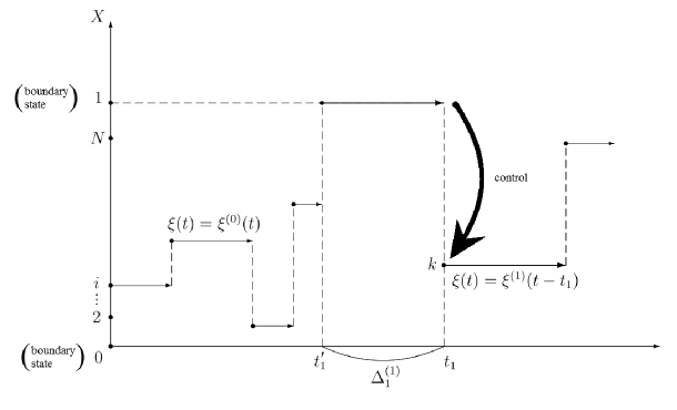
Figure 1: Trajectory of the semi-Markov process $\xi(t)$ controlled at the moments of hitting the boundary of a given subset of the state set.

The corresponding discrete-time stochastic model is constructed similarly. Instead of the semi-Markov process $\xi^{(n)}(t)$, $n=0,1,2,\dots$, we use independent absorbing Markov chains $\xi^{(n)}=\left\{\xi_{t}^{(n)},~{}t=0,1,2,\dots\right\}$, $n=0,1,2,\dots$, ranging in the above-defined state set $X$ with the same transition probability matrix P. We note that, in the discrete-time model, the durations of a single stay in all states can conditionally be assumed to be $1$. Therefore, the random variables $\{\Delta_{n}^{(0)}$, $n=0,1,2,\dots\}$ and $\{\Delta_{n}^{(1)}$, $n=0,1,2,\dots\}$ describing the control action duration are also formally equal to $1$.

The optimal control problem in both versions of the above-described model is formally posed as the extremum problem on the set of pairs of discrete probability distributions $\left(\alpha^{(0)},\alpha^{(1)}\right)$ with respect to a certain stationary cost index of efficiency which has the meaning of the mean specific profit.

3 General probability characteristics of the model

In this section, we determine all probability and cost characteristics required to solve the optimal control problems in both versions of the model under study. We divide these characteristics into initial or primary, which must be given to describe the model, and secondary, which can be expressed in terms of the primary ones using the well-known theoretical assertions. We begin with determining the initial (primary) characteristics.

We let P denote the transition probability matrix for the absorbing Markov chain embedded in the semi-Markov process $\xi^{(n)}(t)$, $n=0,1,2,\dots$. As is known in the theory of absorbing Markov chains [12], such a matrix has the following block structure

$$\textbf{P}=\left(\;\begin{matrix}\textbf{P}_{11}&\textbf{P}_{10}\cr\textbf{P}_{01}&\textbf{P}_{00}\cr\end{matrix}\;\right),$$

where $\textbf{P}_{00}$ is the transition probability matrix inside the set of irreversible admissible states $\{2,3,\dots,N\}$;

$\textbf{P}_{01}$ is the probability matrix for the transitions from the set of admissible states $\{2,3,\dots,N\}$ into the set of absorbing boundary states $\{0,1\}$;

$\textbf{P}_{10}$ is the zero matrix corresponding to transitions from absorbing states $\{0,1\}$ into the set of admissible states $\{2,3,\dots,N\}$;

$\textbf{P}_{11}$ is the unit matrix corresponding to transitions inside the set of absorbing states $\{0,1\}$.

For the discrete-time model, we preserve the above-introduced notation for the transition probability matrices for the independent absorbing Markov chains $\xi^{(n)}$, $n=0,1,2,\dots$.

For the other primary characteristics, we use two types of notation distinguishing the corresponding characteristics of the discrete-time model by the symbol “$~{}\widehat{~{}}~{}$” above a letter. Let us introduce these characteristics in succession:

$\tau_{k}$ is the mathematical expectation (mean) of the time of stay of the semi-Markov process $\xi^{(n)}(t)$ in the state $k\in\{2,3,\dots,N\}$. According to the above remarks, there are no such quantities in the discrete-time model;

$c_{k}$ is the mathematical expectation of the income obtained during the total time of a single stay of the semi-Markov process $\xi^{(n)}(t)$ in the state $k\in\{2,3,\dots,N\}$; in the discrete-time model, the corresponding quantities are denoted by $\widehat{c}_{k}$, $k\in\{2,3,\dots,N\}$, and they characterize the value of the income obtained during a single stay of the Markov chain in the state $k\in\{2,3,\dots,N\}$;

$d_{k}^{(0)}$ and $d_{k}^{(1)}$ are the mathematical expectations of costs due to the control action, i.e., to the transfer of the basic process from the boundary states $\{0,1\}$ into a state $k\in\{2,3,\dots,N\}$. In the discrete-time model, the corresponding characteristics are denoted by $\widehat{d}_{k}^{~{}(0)}$ and $\widehat{d}_{k}^{~{}(1)}$, $k\in\{2,3,\dots,N\}$; according to the economic content of these quantities, we assume that they are negative;

$\mu_{k}^{(0)}$ and $\mu_{k}^{(1)}$ are mathematical expectations of the time necessary to apply the control action, i.e., to transfer the basic process from the boundary states $\{0,1\}$ into a state $k\in\{2,3,\dots,N\}$. In the discrete-time model, such characteristics are absent, because such transitions are realized at one step of the model.

Now let us determine the secondary characteristics. To express these characteristics in terms of primary ones, we use the theoretical results for Markov chains with absorption mainly following the work [12].

By $\textbf{M}=\left(m_{ij}\right)$ we denote the matrix given by the formula $\textbf{M}=\left(\textbf{I}-\textbf{P}_{00}\right)^{-1}$. The entries of this matrix $m_{ij}$ are the mathematical expectations of the number of inputs of the Markov chain embedded in the semi-Markov process $\xi^{(n)}(t)$ into a state $j\in\{2,3,\dots,N\}$ during the time till the moment of absorption, which are determined under the condition that this chain starts to evolve from a state $i\in\{2,3,\dots,N\}$. The corresponding mathematical expectations for the discrete-time model are denoted by $\widehat{m}_{ij}$, $i,j\in\{2,3,\dots,N\}$. These quantities are entries of the matrix $\widehat{\textbf{M}}=\left(\widehat{m}_{ij}\right)$ given by a similar formula.

Let $m_{i}$ be the mathematical expectation of the time from the beginning of the process $\xi^{(n)}(t)$ evolution to the moment of absorption, which is determined under the condition that the initial state is $i$. The corresponding mathematical expectation in the discrete-time model is denoted by $\widehat{m}_{i}$, $i\in\{2,3,\dots,N\}$. These quantities are given by the formulas

$$m_{i}=\sum\limits_{j=2}^{N}m_{ij}\tau_{j},~{}i\in\{2,3,\dots,N\},$$ (8)

$$\widehat{m}_{i}=\sum\limits_{j=2}^{N}\widehat{m}_{ij},~{}i\in\{2,3,\dots,N\}.$$ (9)

By $r_{i}$ we denote the mathematical expectation of the income due to the evolution of the process $\xi^{(n)}(t)$ till the absorption, which is determined under the condition that the initial state is $i$, $i\in\{2,3,\dots,N\}$. The corresponding mathematical expectation in the discrete-time model is denoted by $\widehat{r}_{i}$, $i\in\{2,3,\dots,N\}$. These quantities are determined by the formulas ([4,12])

$$r_{i}=\sum\limits_{j=2}^{N}m_{ij}c_{j},~{}i\in\{2,3,\dots,N\};$$ (10)

$$\widehat{r}_{i}=\sum\limits_{j=2}^{N}\widehat{m}_{ij}\widehat{c}_{j},~{}i\in\{2,3,\dots,N\}.$$ (11)

Further, we let $b_{i0}$ and $b_{i1}$ denote the conditional probabilities of the events that the semi-Markov process $\xi^{(n)}(t)$ is absorbed in the respective state $0$ or $1$, which are determined under the condition that the initial state of the process is $i\in\{2,3,\dots,N\}$. We let the vectors $(b_{i0}$ and $b_{i1})$, $i\in\{2,3,\dots,N\}$, form a $(N-1)\times 2$ matrix B.

Then we have the formula [12]

$$\textbf{B}=(\textbf{I}-\textbf{P}_{00})^{-1}\textbf{P}_{01}=\textbf{MP}_{01}.$$ (12)

The corresponding probabilities for the discrete-time model are denoted by $\widehat{b}_{i0}$ and $\widehat{b}_{i1}$, $i\in\{2,3,\dots,N\}$. They are entries of the matrix $\widehat{\textbf{B}}=\left(\widehat{b}_{i0},~{}\widehat{b}_{i1},~{}~{}i\in\{2,3,\dots,N\}\right)$, which is given by a similar formula

$$\widehat{\textbf{B}}=\left(I-P_{00}\right)^{-1}P_{01}=\widehat{\textbf{M}}P_{01}.$$ (13)

Thus, the secondary probability characteristics of continuous- and discrete-time models, given by formulas (8)–(13), can explicitly be expresses in terms of the initial (primary) characteristics. This means that to solve the optimal control problems in these models, it suffices to prescribe only a set of primary characteristics.

4 Analytic representation of stationary
cost indices of the control quality

Now we consider the stationary cost index of the control efficiency related to the evolution of this stochastic model. We note that the nature of such an index is the same in both versions of the model, with continuous time and with discrete time. From the formal standpoint, this index is the limit

$$I=\lim\limits_{t\rightarrow\infty}\dfrac{V(t)}{t},$$

where $V(t)$ is the mathematical expectation of an additive functional (accumulation functional) defined on the trajectory of the stochastic process under study.

According to its economic content, the index $I$ is the mean specific profit obtained as the system operates under stationary conditions. Such indices have been known since the fundamental studies in the theory of control of Markov and semi-Markov stochastic processes [3,4]. We note that similar indices are used in contemporary studies [5,6].

We use ergodic theorems for Markov and semi-Markov stochastic processes to obtain explicit analytic representations for such indices in both versions of the stochastic model considered in this paper. For continuous-time models, one can use the assertion proved in [4], Chapter 5, Section 5.5, or the corresponding assertions for general semi-Markov models with arbitrary state spaces and controls [5,6]. For discrete-time models, one can use the classical ergodic theorem for Markov chains ([13], Chapter 8]).

Remark 2.

To apply the above-cited ergodic theorems, it is necessary to require that the constructed continuous- and discrete-time stochastic models have a certain property which can be called stability. For continuous-time models, this means that the probabilities of absorption for any initial state $i\in\{2,3,\dots,N\}$ must satisfy the conditions $b_{i0}>0$, $b_{i1}>0$, and $b_{i0}+b_{i1}=1$. Then the absorbing boundary states are admissible from any initial state $i$ with probability $1$.

Now we consider an auxiliary Markov chain with the state set $\{0,1\}$, which is formed by the values of the process at the moments of hitting the boundary states $\xi^{\prime}_{n}=\xi(t^{\prime}_{n})$, $n=0,1,2,\dots$. Under these conditions, this chain is irreducible and has a unique stationary distribution. [The classical theory of Markov chains is discussed in detail in [8], Chapter VIII; also see the above-cited work [13], Chapter 8.] At the same time, the additive cost functional $V(t)$ determining the control efficiency index $I$ can be defined on the trajectories of precisely this Markov chain. According to the above-cited ergodic theorems, the limits $I=\lim\limits_{t\rightarrow\infty}\big{[}\frac{V(t)}{t}\big{]}$ exist. All quantities entering the explicit representation for $I$ are expressed in terms of the initial (primary and secondary) characteristics of the model. Similar remarks also remain true for the discrete-time model.

Now we formulate assertions about analytic representations of stationary cost indices of the control efficiency in terms of the well-known primary and secondary probability characteristics of the model and the discrete probability distributions $\alpha^{(0)}$ and $\alpha^{(1)}$ describing the control actions. The following assertion holds for the continuous-time model.

Theorem 2.

The stationary index of the mean specific profit has the analytic representation

$$I=\dfrac{\sum\limits_{k=2}^{N}\alpha_{k}^{(0)}\left[d_{k}^{(0)}+r_{k}\right]\sum\limits_{l=2}^{N}\alpha_{l}^{(1)}b_{l0}+\sum\limits_{k=2}^{N}\alpha_{k}^{(1)}\left[d_{k}^{(1)}+r_{k}\right]\sum\limits_{l=2}^{N}\alpha_{l}^{(0)}(1-b_{l0})}{\sum\limits_{k=2}^{N}\alpha_{k}^{(0)}\left[\mu_{k}^{(0)}+m_{k}\right]\sum\limits_{l=2}^{N}\alpha_{l}^{(1)}b_{l0}+\sum\limits_{k=2}^{N}\alpha_{k}^{(1)}\left[\mu_{k}^{(1)}+m_{k}\right]\sum\limits_{l=2}^{N}\alpha_{l}^{(0)}(1-b_{l0})}.$$ (14)

The corresponding assertion for the discrete-time model can be formulated as follows.

Theorem 3.

The stationary index of the mean specific profit can be represented as

$$\widehat{I}=\dfrac{\sum\limits_{k=2}^{N}\alpha_{k}^{(0)}\left[\widehat{d}_{k}^{~{}(0)}+\widehat{r}_{k}\right]\sum\limits_{l=2}^{N}\alpha_{l}^{(1)}\widehat{b}_{l0}+\sum\limits_{k=2}^{N}\alpha_{k}^{(1)}\left[\widehat{d}_{k}^{~{}(1)}+\widehat{r}_{k}\right]\sum\limits_{l=2}^{N}\alpha_{l}^{(0)}(1-\widehat{b}_{l0})}{\sum\limits_{l=2}^{N}\alpha_{l}^{(1)}\widehat{b}_{l0}+\sum\limits_{l=2}^{N}\alpha_{l}^{(0)}(1-\widehat{b}_{l0})}.$$ (15)

Remark 3.

The continuous- and discrete-time stochastic models under study can be generalized by assuming that the set of boundary states is an arbitrary finite set. In this case, the states contained in it are called external states with respect to the internal admissible states. The auxiliary Markov chain formed by the values of the process at the moments of transition to external states has finitely many states. Under natural assumptions similar to those formulated in Remark 2, this chain is irreducible and has a unique stationary distribution. The control actions are determined by finitely many probability distributions each of which described the transitions from a certain external state into an internal (admissible) state. For such models, one can prove assertions similar to Theorems 2 and 3. In this case, expressions (14) and (15) contain stationary probabilities of the auxiliary Markov chains mentioned above. In turn, these stationary probabilities are solutions of systems of linear algebraic equations and can be expressed in terms of the initial probability characteristics of stochastic models.

5 Solution of the optimal control problem

Now to complete the study, we present the solution of the optimal control problems in both versions of the stochastic model. For this, we represent the stationary cost indices of the control quality, given by formulas (14) and (15), as linear-fractional integral functionals of discrete probability distributions $\alpha^{(0)}$ and $\alpha^{(1)}$. We use analytic transformations of formula (14) to prove the following assertion for the continuous-time model.

Theorem 4.

The stationary cost index $I(\alpha^{(0)},\alpha^{(1)})$ given by formula (14) can be represented as a discrete linear-fractional integral functional of the probability distributions $\alpha^{(0)},\alpha^{(1)}$, namely,

$$I(\alpha^{(0)},\alpha^{(1)})=\dfrac{\sum\limits_{l_{0}=2}^{N}\sum\limits_{l_{1}=2}^{N}A(l_{0},l_{1})\alpha_{l_{0}}^{(0)}\alpha_{l_{1}}^{(1)}}{\sum\limits_{l_{0}=2}^{N}\sum\limits_{l_{1}=2}^{N}B(l_{0},l_{1})\alpha_{l_{0}}^{(0)}\alpha_{l_{1}}^{(1)}},$$ (16)

$$\text{where}~{}A(l_{0},l_{1})=\left[d_{l_{0}}^{(0)}+r_{l_{0}}\right]b_{l_{1},0}+\left[d_{l_{1}}^{(1)}+r_{l_{1}}\right]b_{l_{0},1},$$ (17)

$$B(k_{0},k_{1})=\left[\mu_{l_{0}}^{(0)}+m_{l_{0}}\right]b_{l_{1},0}+\left[\mu_{l_{1}}^{(1)}+m_{l_{1}}\right]b_{l_{0},1}.$$ (18)

It follows from Theorem 4 that the test function of the discrete linear-fractional integral functional (16) is given by the relation

$$C(l_{0},l_{1})=\dfrac{A(l_{0},l_{1})}{B(l_{0},l_{1})},$$ (19)

where the functions $A(l_{0},l_{1})$ and $B(l_{0},l_{1})$ are respectively determined by formulas (17) and (18).

A similar assertion, which can be proved by using analytic transformations of formula (15), also holds for the discrete-time model.

Theorem 5.

The stationary cost index $\widehat{I}\left(\alpha^{(0)},\alpha^{(1)}\right)$ given by formula (15) can be represented as a discrete linear-fractional integral functional of the probability distributions $\alpha^{(0)}$ and $\alpha^{(1)}$, namely,

$$\widehat{I}\left(\alpha^{(0)},\alpha^{(1)}\right)=\dfrac{\sum\limits_{l_{0}=2}^{N}\sum\limits_{l_{1}=2}^{N}\widehat{A}(l_{0},l_{1})\alpha_{l_{0}}^{(0)}\alpha_{l_{1}}^{(1)}}{\sum\limits_{l_{0}=2}^{N}\sum\limits_{l_{1}=2}^{N}\widehat{B}(l_{0},l_{1})\alpha_{l_{0}}^{(0)}\alpha_{l_{1}}^{(1)}},$$ (20)

where

$$\widehat{A}(l_{0},l_{1})=\left[\widehat{d}_{l_{0}}^{~{}(0)}+\widehat{r}_{l_{0}}\right]\widehat{b}_{l_{1},0}+\left[\widehat{d}_{l_{1}}^{~{}(1)}+\widehat{r}_{l_{1}}\right]\widehat{b}_{l_{0},1},$$ (21)

$$\widehat{B}(l_{0},l_{1})=\widehat{b}_{l_{1},0}+\widehat{b}_{l_{0},1}.$$ (22)

It follows from the assertion of Theorem 5 that the test function of the discrete linear-fractional integral functional (20) has the form

$$\widehat{C}(l_{0},l_{1})=\dfrac{\widehat{A}(l_{0},l_{1})}{\widehat{B}(l_{0},l_{1})},$$ (23)

where the functions $\widehat{A}(l_{0},l_{1})$ and $\widehat{B}(l_{0},l_{1})$ are determined by formulas (21) and (22), respectively.

The optimal control problems for continuous- and discrete-time models are formulated in the form of extremum problems (3) posed on the set $\Gamma_{d}$ which consists of pairs of all possible discrete probability distributions $\left(\alpha^{(0)},~{}\alpha^{(1)}\right)$ with respect to functionals (16) and (20), respectively. In this case, the sets of admissible controls $U_{0}$ and $U_{1}$ are determined as $U_{0}=U_{1}=\{2,3,\dots,N\}$, and the set $U$ is the Cartesian product $U=U_{0}\times U_{1}=\left\{(l_{0},l_{1}),~{}l_{0}\in U_{0},~{}l_{1}\in U_{1}\right\}$. To solve these problems, it is necessary to use Theorem 1. We note that the conditions of Theorem 1 are satisfied in both problems. In particular, the functions $B(l_{0},l_{1})$ and $\widehat{B}(l_{0},l_{1})$ are strictly positive for all $(l_{0},l_{1})\in U$.

If the set of admissible controls $U_{0}=U_{1}=\{2,3,\dots,N\}$ is finite, then the test functions of the discrete linear-fractional integral functionals $C(l_{0},l_{1})$ and $\widehat{C}(l_{0},l_{1})$, given by formulas (19) and (23), attain the global extrema (maximum and minimum). Then, it follows from Theorem 1 that the solution of the optimal control problems exists for any of the model. The optimal controls for both models are deterministic and are determined by the points at which the test functions attain their global maxima. If the set of admissible controls $U_{0}=U_{1}=\{2,3,\dots,N\}$ is countable ($N=\infty$), then the solutions of extremum problems for continuous- and discrete-time models are also completely determined by the extremum properties of the test functions $C(l_{0},l_{1})$ and $\widehat{C}(l_{0},l_{1})$, as it follows from the general assertion about an extremum of the linear-fractional integral functional ([1], Theorem 1). Thus, this theorem is a theoretical foundation which permits obtaining the complete solution of the tuning problem for the stochastic models considered above.

Concluding remarks

In the study whose main results are described in the present paper, we developed a general concept of stochastic model with controls applied at the moments when the basic process hits the boundary of a given subset of the state set. The proposed concept is realized for two versions of the initial stochastic model: the version based on the use of a continuous-time semi-Markov process with embedded absorbing Markov chain and the version based on the use of a discrete-time Markov process with absorbing states. For both versions of the model, we pose and solve the optimal control problems, i.e., the corresponding tuning problems. The theoretical background of such solutions is the theorem about an unconditional extremum of a linear-fractional integral functional [1], which, in the discrete version, becomes Theorem 1 in Section 1.

We note that the possible constructions of new versions of the general stochastic model with controls at the moments of hitting the boundary of a given subset of the state set are far from being complete. We distinguish several fundamental conditions necessary to construct such well-posed and meaningful versions.

1. The set of states must contain a given subset of the so-called admissible states and a finite subset of states which we conditionally call external or boundary states with respect to the admissible states. In this case, the set of admissible states need not be discrete.

2. A certain general condition related to the behavior of the initial stochastic process $\xi^{(n)}(t)$ (continuous time) or $\xi^{(n)}$ (discrete time) must be satisfied. This condition means that this stochastic process, which starts to evolve from an arbitrary admissible state, must get into one of the external (boundary) states in a finite time with probability $1$.

3. The Markov property must be satisfied at the moments of transition into external (boundary) states and at the moments of output from external states and transition into one of the states in the admissible set.

4. The probability characteristics describing the transition from an arbitrary fixed admissible state into one of the external states (an analog of the absorption probabilities) can be determined analytically.

5. The mathematical expectations of the time passed from leaving an arbitrary fixed admissible state and entering one of the external states and the mathematical expectations of the income accumulated in this time can be determined analytically.

We note that conditions 1–3 in this set of conditions are related to the general stochastic properties of the model. Conditions 4 and 5 must ensure the possibility of determining the analytic representations for the required probability characteristics of the basic process which are related to the time of its stay in the set of admissible states.

Under the above-listed conditions, one can construct a stochastic model with controls similar to the models which were considered in this study and obtain an explicit representation for the stationary cost index of the control efficiency and the complete solution of the corresponding tuning problem.

References

- [1] V. P. Shnurkov, “Solution of the unconditional extremum problem for a linear-fractional integral functional on a set of probability measures,” Dokl. Ross. Akad. Nauk 470 (4), 387–392 (2016) [Dokl. Math.].
- [2] V. P. Shnurkov, A. K. Gorshenin, and V. V. Belousov, “Analytic solution of optimal control problem for semi-Markov process with a finite set of states,” Informatika i Primeneniya 10 (4), 72–88 (2016).
- [3] W. S. Jewell, “Markov-Renewal Programming. I, II.” Operations Research 11 (6), 938–971 (1963).
- [4] H. Mine and S. Osaki, Markovian Decision Processes (Amer. Elsevier, New York, 1970).
- [5] F. Luque-Vasquez and O. Herndndez-Lerma, “Semi-Markov control models with average costs,” Appl. Math. 26 (3), 315–331 (1999).
- [6] O. Vega-Amaya and F. Luque-Vasquez, “Sample-path average cost optimality for semi-Markov control processes on Borel spaces: Unbounded costs and mean holding times,” Appl. Math. 27 (3), 343–367 (2000).
- [7] P. Halmos, Measure Theory (Litton, New York, 1950; Springer-Verlag, New York, 1974).
- [8] A. N. Shiryaev, Probability (Springer, 2016).
- [9] A. A. Borovkov, Probability Theory (Springer. 2013).
- [10] V. S. Korolyuk and A. F. Turbin, Semi-Markov Processes and Their Applications (Naukova Dumka, Kiev, 1976) [in Russian].
- [11] J. Janssen and R. Manca, Applied Semi-Markov Processes (Springer, New York, 2006).
- [12] J. Kemeny and J. Snell, Finite Markov Chains (Prentice–Hall, 1959).
- [13] V. S. Korolyuk, N. I. Portenko, A., V. Skorokhod, and A. F. Turbin, Handbook in Probability and Mathematical Statistics, Ed. by V. S. Korolyuk (Naukova Dumka, Kiev, 1995) [in Russian].