We investigate inflation models in Jordan frame supergravity, in which an inflaton non-minimally couples to the scalar curvature. By imposing the condition that an inflaton would have the canonical kinetic term in the Jordan frame, we construct inflation models with asymptotically flat potential through pole inflation technique and discuss their relation to the models based on Einstein frame supergravity. We also show that the model proposed by Ferrara et al. has special position and the relation between the Kähler potential and the frame function is uniquely determined by requiring that scalars take the canonical kinetic terms in the Jordan frame and that a frame function consists only of a holomorphic term (and its anti-holomorphic counterpart) for symmetry breaking terms. Our case corresponds to relaxing the latter condition.

1 Introduction

The observations of cosmic microwave background (CMB) radiation anisotropies [1, 2] strongly support the presence of inflation in the very early Universe and also constrain the property of primordial perturbations. Though primordial tensor perturbations have not yet been observed unfortunately, primordial curvature perturbations are well constrained on CMB scales [3, 4]. These constraints favor the Starobinsky [5] and the Higgs inflation models [6, 7], which suggest the $\alpha$-attractor models [8, 9, 10] and the $\xi$-models [11, 12, 13, 14], and these models are finally understood as pole inflation [15, 16] in a unified manner. The pole inflation approach was further generalized in Ref. [17], and applied to supergravity based models in Refs. [18, 19].

The Higgs inflation model (and the Starobinsky model after introducing the Lagrangian multiplier field) works well by introducing a non-minimal coupling to the scalar curvature. Of course, by conformal transformation [20], we can have an equivalent system, in which a scalar field minimally couples to gravity. Thus, we can freely interchange the Jordan frame with the Einstein frame as long as a conformal factor is positive definite and there is no preferred frame in principle [21, 22, 23, 24, 25, 26]. Then, one of strong motivations to introduce such a non-minimal coupling (Jordan frame) is to easily realize (apparently) complicated potential in the Einstein frame from simple potential in the Jordan frame [27]. Actually, in the Higgs inflation model, the Higgs field has quartic power-law potential (in the large field approximation) in the Jordan frame, which is converted to an asymptotically flat potential in the Einstein frame.

This kind of analysis was done in the context of superconformal supergravity. Though LHC has not yet found the supersymmetry unfortunately, it is still expected to exist at the very high energy scale where inflation happened because it can control quantum corrections to an inflaton. Based on the superconformal supergravity [28], Ferrara et al. derived a $N=1,d=4$ supergravity action in the Jordan frame [29]. They also found [29, 30] that a special class of the Kähler potential and the frame function gives rise to the canonical kinetic terms of scalar fields in the Jordan frame. Based on this formalism, they discussed various aspects of inflation in the next-to-minimal supersymmetric Standard Model (NMSSM), which is included in this class.

In this paper, we first show that the model proposed in Refs. [29, 30] has special position and that the relation between the Kähler potential and the frame function is uniquely determined by requiring that scalars take the canonical kinetic terms in the Jordan frame and the frame function consists only of a holomorphic term (and its anti-holomorphic counterpart) except the conformal part. Based on this observation, we relax the latter condition with keeping the canonical kinetic term of scalar field in the Jordan frame and construct inflation models with asymptotically flat potential in the Einstein frame by use of pole inflation structure.

The organization of the paper is as follows. In the next section, after briefly reviewing the Jordan frame supergravity obtained from adequate gauge fixing on superconformal supergravity [29, 30], we explicitly show that, in the model proposed by Ferrara et al., the relation between the Kähler potential and the frame function is uniquely determined by imposing adequate conditions. In Sec. 3, we review the implications of this model and discuss its possible generalizations. In Sec. 4, after introducing the pole inflation approach, we relax the condition proposed by Refs. [29, 30], and consider the non-holomorphic frame function with keeping the canonical kinetic term of scalar field in the Jordan frame. It is shown that even for such relaxed conditions we can obtain asymptotically flat inflaton potential through pole inflation technique. The relation to the models based on Einstein frame supergravity is also discussed. Final section is devoted to summary and discussions.

2 Jordan frame supergravity

In this section, we briefly review the Jordan frame supergravity according to Refs. [29, 30]. After describing the bosonic part of the supergravity action in the Jordan frame, we explicitly show that the model proposed by Ferrara et al. [29] is special in that the relation between the Kähler potential and the frame function is uniquely determined by assuming that scalars take the canonical kinetic terms in the Jordan frame and that the frame function consists only of a holomorphic term (and its anti-holomorphic counterpart) except the conformal part. Hereafter we take the unit of $M_{\rm Pl}=1$ unless otherwise stated, where $M_{\rm Pl}$ is the reduced Planck mass.

2.1 Supergravity action in the Jordan frame

The action in the Jordan frame supergravity is specified by four functions, the Kähler potential $\mathcal{K}(z,\bar{z})$, superpotential $W(z)$, gauge kinetic function $f_{AB}(z)$, and frame function $\Phi(z,\bar{z})$. The bosonic part of the Lagrangian density in the Jordan frame is given by [29]

$$\frac{\mathcal{L}}{\sqrt{-g_{J}}} =-\frac{1}{6}\Phi\mathcal{R}_{J}+\left(\frac{1}{3}\Phi g_{\alpha\bar{\beta}}-\frac{\Phi_{\alpha}\Phi_{\bar{\beta}}}{\Phi}\right)g_{J}^{\mu\nu}\hat{\partial}_{\mu}z^{\alpha}\hat{\partial}_{\nu}\bar{z}^{\bar{\beta}}$$

$$\quad-\frac{1}{4\Phi}\left(\Phi_{\alpha}\hat{\partial}_{\mu}z^{\alpha}-\Phi_{\bar{\beta}}\hat{\partial}_{\mu}\bar{z}^{\bar{\beta}}\right)\left(\Phi_{\gamma}\hat{\partial}_{\nu}z^{\gamma}-\Phi_{\bar{\delta}}\hat{\partial}_{\nu}\bar{z}^{\bar{\delta}}\right)g_{J}^{\mu\nu}-V_{J}+\mathcal{L}_{1},$$ (2.1)

where

$$\hat{\partial}_{\mu}z^{\alpha}=\partial_{\mu}z^{\alpha}-A_{\mu}^{A}k_{A}^{\alpha}$$ (2.2)

are gauge covariant derivatives of scalar fields $z^{\alpha}$ with $\alpha=1,\dots,n$ for the theory including $n$ supermultiplets, $A_{\mu}^{A}$ are Yang-Mills gauge fields with $A$ representing the gauge indices, $k_{A}^{\alpha}$ are Killing vectors of the Kähler manifold, $\mathcal{R}_{J}$ is the scalar curvature obtained from the Jordan frame metric $g_{J\mu\nu}$,

$$g_{\alpha\bar{\beta}}=\frac{\partial}{\partial z^{\alpha}}\frac{\partial}{\partial\bar{z}^{\bar{\beta}}}\mathcal{K}(z,\bar{z})$$ (2.3)

is the Kähler metric, and

$$\Phi_{\alpha}\equiv\frac{\partial}{\partial z^{\alpha}}\Phi,\quad\Phi_{\bar{\beta}}\equiv\frac{\partial}{\partial\bar{z}^{\bar{\beta}}}\Phi.$$ (2.4)

Here, $\mathcal{L}_{1}$ contains the kinetic terms of gauge fields,

$$\mathcal{L}_{1}=-\frac{1}{4}(\mathrm{Re}f_{AB})F^{A}_{\mu\nu}F^{\mu\nu B}+\frac{i}{4}(\mathrm{Im}f_{AB})F^{A}_{\mu\nu}\tilde{F}^{\mu\nu B},$$ (2.5)

which is conformal invariant and takes the same form both in the Jordan frame and the Einstein frame. The scalar potential is given by

$$V_{J} =\frac{1}{9}\Phi^{2}V_{E},$$ (2.6)

$$V_{E} =V_{E}^{F}+V_{E}^{D},$$ (2.7)

$$V_{E}^{F} =e^{\mathcal{K}}\left(-3W\bar{W}+g^{\alpha\bar{\beta}}\nabla_{\alpha}W\nabla_{\bar{\beta}}\bar{W}\right),$$ (2.8)

$$V_{E}^{D} =\frac{1}{2}(\mathrm{Re}f)^{-1\ AB}P_{A}P_{B},$$ (2.9)

where

$$\nabla_{\alpha}W =\partial_{\alpha}W+(\partial_{\alpha}\mathcal{K})W,$$ (2.10)

$$P_{A}(z,\bar{z}) =i(k_{A}^{\alpha}\partial_{\alpha}\mathcal{K}-r_{A})=-i(k_{A}^{\bar{\alpha}}\partial_{\bar{\alpha}}\mathcal{K}-\bar{r}_{A}),$$ (2.11)

and the holomorphic function $r_{A}(z)$ becomes nonzero only if the Kähler potential changes nontrivially under Yang-Mills gauge transformations.

We can move into the Einstein frame by performing the following reparameterization in Eq. (2.1)

$$g_{J}^{\mu\nu}=\Omega^{2}g_{E}^{\mu\nu},\quad\Omega^{2}=-\frac{1}{3}\Phi.$$ (2.12)

By using the following relations

$$\sqrt{-g_{J}} =\Omega^{-4}\sqrt{-g_{E}},$$ (2.13)

$$\mathcal{R}_{J} =\Omega^{2}\left(\mathcal{R}_{E}+6\Box_{E}\ln\Omega-6g_{E}^{\mu\nu}\partial_{\mu}(\ln\Omega)\partial_{\nu}(\ln\Omega)\right),$$ (2.14)

$$\Box_{E}\ln\Omega =\frac{1}{\sqrt{-g_{E}}}\partial_{\mu}\left(\sqrt{-g_{E}}g_{E}^{\mu\nu}\partial_{\nu}\ln\Omega\right),$$ (2.15)

where $\mathcal{R}_{E}$ is the scalar curvature obtained from the Einstein frame metric $g_{E\mu\nu}$, we obtain the Lagrangian in the Einstein frame (up to the total derivative)

$$\frac{\mathcal{L}}{\sqrt{-g_{E}}}=\frac{1}{2}\mathcal{R}_{E}-g_{\alpha\bar{\beta}}g_{E}^{\mu\nu}\hat{\partial}_{\mu}z^{\alpha}\hat{\partial}_{\nu}\bar{z}^{\bar{\beta}}-V_{E}+\mathcal{L}_{1}.$$ (2.16)

Note that the Einstein frame action does not depend on the function $\Phi(z,\bar{z})$. The kinetic terms of scalar fields are solely determined by the Kähler potential $\mathcal{K}(z,\bar{z})$.

The complete $N=1$ supergravity action including fermions in an arbitrary Jordan frame was obtained in Ref. [29] by applying superconformal approach to supergravity [28]. In this approach, the Jordan frame action which is invariant under the super-Poincaré algebra is derived by gauge fixing all extra symmetries in the superconformal algebra. In this gauge-fixing procedure, the basis of chiral supermultiplets $\{X^{I}\}$ in the superconformal theory is changed into a basis $\{y,z^{\alpha}\}$, where $y$ transforms under dilatations, but $z^{\alpha}$ do not transform under them. After applying the gauge condition, $y$ is no longer a dynamical field and becomes a non-holomorphic function of other physical scalar fields $z^{\alpha}$. In particular, the gauge condition used in Ref. [29] reads

$$y=\bar{y}=\sqrt{-\frac{\Phi}{3}}\exp\frac{\mathcal{K}}{6}.$$ (2.17)

This implies that $y$ and $\bar{y}$ are determined as a function of $z^{\alpha}$ and $\bar{z}^{\bar{\alpha}}$ once we specify $\mathcal{K}$ and $\Phi$. It will be convenient to rewrite the above equation as

$$\mathcal{K}(z,\bar{z})=-3\log\left(-\frac{1}{3}\frac{\Phi(z,\bar{z})}{Y(z,\bar{z})}\right),$$ (2.18)

where we introduced a function $Y(z,\bar{z})\equiv y(z,\bar{z})\bar{y}(z,\bar{z})$.

2.2 FKLMP formulation

Ferrara, Kallosh, Linde, Marrani, and Van Proeyen (FKLMP) [29] proposed the following conditions to obtain canonical kinetic terms for scalar fields in the Jordan frame:

1. The frame function and the Kähler potential have the following relation

   $$\mathcal{K}(z,\bar{z})=-3\log\left(-\frac{1}{3}\Phi(z,\bar{z})\right).$$ (2.19)

   This condition corresponds to the fact that we arrange the Kähler potential such that $Y(z,\bar{z})$ becomes unity in Eq. (2.18).

2. The frame function takes the following form

   $$\Phi(z,\bar{z})=-3+\delta_{\alpha\bar{\beta}}z^{\alpha}\bar{z}^{\bar{\beta}}+J(z)+\bar{J}(\bar{z}),$$ (2.20)

   where $J(z)$ is a holomorphic function, and the scalar field configuration satisfies the following condition

   $$\mathcal{A}_{\mu}=0.$$ (2.21)

   Here, $\mathcal{A}_{\mu}$ is given by

   $$\mathcal{A}_{\mu}=-\frac{i}{2\Phi}\left(\Phi_{\alpha}\hat{\partial}_{\mu}z^{\alpha}-\Phi_{\bar{\beta}}\hat{\partial}_{\mu}\bar{z}^{\bar{\beta}}\right),$$ (2.22)

   which corresponds to the auxiliary field in the superconformal formulation of supergravity.

Indeed, if we substitute Eq. (2.19) into Eq. (2.1), the Jordan frame Lagrangian becomes

$$\mathcal{L}_{\rm FKLMP}=\sqrt{-g_{J}}\left[-\frac{1}{6}\Phi\mathcal{R}_{J}-\Phi_{\alpha\bar{\beta}}\hat{\partial}_{\mu}z^{\alpha}\hat{\partial}_{\nu}\bar{z}^{\bar{\beta}}g_{J}^{\mu\nu}+\Phi\mathcal{A}_{\mu}^{2}-V_{J}+\mathcal{L}_{1}\right].$$ (2.23)

Then it reduces to the form with canonical kinetic terms for scalar fields when we apply conditions given by Eqs. (2.20) and (2.21).

It should be noticed, as mentioned in [29], that this set of the frame function and the Kähler potential (together with $\mathcal{A}_{\mu}=0$) is sufficient to give the canonical kinetic terms of scalar fields in the Jordan frame. These conditions, however, seem to be ad hoc, and there might be a room to extend, since in general we can use Eq. (2.18) for the Kähler potential rather than Eq. (2.19). Furthermore, it might be possible to use the following frame function,

$$\Phi(z,\bar{z})=-3+\delta_{\alpha\bar{\beta}}z^{\alpha}\bar{z}^{\bar{\beta}}+\mathcal{J}(z,\bar{z}),$$ (2.24)

where $\mathcal{J}(z,\bar{z})$ is an arbitrary function of $z^{\alpha}$ and $\bar{z}^{\bar{\alpha}}$. In Sec. 3 we will argue that this $\mathcal{J}(z,\bar{z})$ term can be identified as a deformation of the Kähler potential with a specific symmetric structure. The FKLMP model corresponds to the case where the function $\mathcal{J}(z,\bar{z})$ becomes a holomorphic form $J(z)+\bar{J}(\bar{z})$.

Here we explicitly show that the special relation between the Kähler potential and the frame function [Eq. (2.19)] follows from the requirement that the kinetic terms of the scalar fields are canonically normalized and that the $\mathcal{J}(z,\bar{z})$ term in Eq. (2.24) is given by a holomorphic function and its anti-holomorphic counterpart.

The kinetic term in the Jordan frame is given by

$$\frac{\mathcal{L}_{{\rm kin},J}}{\sqrt{-g_{J}}}=\left(\frac{1}{3}\Phi g_{\alpha\bar{\beta}}-\frac{\Phi_{\alpha}\Phi_{\bar{\beta}}}{\Phi}\right)g_{J}^{\mu\nu}\hat{\partial}_{\mu}z^{\alpha}\hat{\partial}_{\nu}\bar{z}^{\bar{\beta}}.$$ (2.25)

In order to have canonical kinetic terms, we require that

$$g_{\alpha\bar{\beta}}=\frac{3}{\Phi}\left(\frac{\Phi_{\alpha}\Phi_{\bar{\beta}}}{\Phi}-\delta_{\alpha\bar{\beta}}\right).$$ (2.26)

From Eq. (2.18), we also have

$$g_{\alpha\bar{\beta}}=-3\left(\frac{\Phi_{\alpha\bar{\beta}}}{\Phi}-\frac{\Phi_{\alpha}\Phi_{\bar{\beta}}}{\Phi^{2}}-\frac{Y_{\alpha\bar{\beta}}}{Y}+\frac{Y_{\alpha}Y_{\bar{\beta}}}{Y^{2}}\right).$$ (2.27)

Combining these two equations, we obtain

$$\frac{\delta_{\alpha\bar{\beta}}}{\Phi}=\frac{\Phi_{\alpha\bar{\beta}}}{\Phi}-\frac{Y_{\alpha\bar{\beta}}}{Y}+\frac{Y_{\alpha}Y_{\bar{\beta}}}{Y^{2}}.$$ (2.28)

If we choose the holomorphic term, $\mathcal{J}(z,\bar{z})=J(z)+\bar{J}(\bar{z})$, Eq. (2.28) reduces to

$$\left(\log Y\right)_{\alpha\bar{\beta}}=0.$$ (2.29)

Since the Kähler potential and hence $\log Y$ should be a real function, the solution of Eq. (2.29) is of the form

$$\log Y=h(z)+\bar{h}(\bar{z})+\mathrm{const.},$$ (2.30)

where $h(z)$ is some holomorphic function. The terms in the right-hand side of Eq. (2.30) can be eliminated by using Kähler transformations. Therefore, we must use the relation given by Eq. (2.19) as long as we assume that the kinetic terms are canonically normalized in the Jordan frame and that the $\mathcal{J}(z,\bar{z})$ term is holomorphic. Conversely, we expect that the relation between $\mathcal{K}(z,\bar{z})$ and $\Phi(z,\bar{z})$ is modified as Eq. (2.18) once we consider some non-holomorphic function for the $\mathcal{J}(z,\bar{z})$ term.

3 Inflation models in Jordan frame supergravity

The implications of the FKLMP formulation in the context of inflationary cosmology were discussed further in Refs. [30, 31]. Before discussing such supergravity based models, let us first consider the following (non-supersymmetric) toy model with two real scalar fields $\chi$ and $\varphi$,

$$\mathcal{L}=\sqrt{-g}\left[\frac{1}{2}\partial_{\mu}\chi\partial_{\nu}\chi g^{\mu\nu}-\frac{1}{2}\partial_{\mu}\varphi\partial_{\nu}\varphi g^{\mu\nu}+\frac{\chi^{2}}{12}\mathcal{R}-\frac{\varphi^{2}}{12}\mathcal{R}-\frac{\lambda}{4}\varphi^{4}\right].$$ (3.1)

$\chi$ has a wrong sign in the kinetic term, but it is not a problem because $\chi$ is the compensator field rather than the physical field. The Lagrangian (3.1) is invariant under the following conformal transformations

$$g_{\mu\nu} \to e^{-2\sigma(x)}g_{\mu\nu},$$

$$\varphi \to e^{\sigma(x)}\varphi,$$

$$\chi \to e^{\sigma(x)}\chi,$$ (3.2)

where $\sigma(x)$ is a position-dependent parameter. If we take the conformal gauge as $\chi=\sqrt{6}$, we obtain the Jordan frame Lagrangian with the single scalar field $\varphi$,

$$\mathcal{L}=\sqrt{-g}\left[\frac{1}{2}\mathcal{R}-\frac{1}{2}\partial_{\mu}\varphi\partial_{\nu}\varphi g^{\mu\nu}-\frac{\varphi^{2}}{12}\mathcal{R}-\frac{\lambda}{4}\varphi^{4}\right].$$ (3.3)

The above Lagrangian contains the non-minimal scalar-curvature coupling $\frac{\xi}{2}\varphi^{2}\mathcal{R}$ with $\xi=-\frac{1}{6}$. On the other hand, in order to explain the observational results through the inflationary model with the quartic potential and non-minimal scalar-curvature coupling $\frac{\xi}{2}\varphi^{2}\mathcal{R}-\frac{\lambda}{4}\varphi^{4}$, generically we need a value $\xi\neq-\frac{1}{6}$. In fact, such a model leads to asymptotically flat potential in the Einstein frame, and it can be shown that a value of $\xi\gtrsim\mathcal{O}(10^{-3})$ is required to explain the observational results [31]. This fact implies that inflation cannot be explained in the above toy model with two real scalar fields and the quartic potential, unless we introduce an explicit breaking of the conformal symmetry ($\xi\neq-\frac{1}{6}$).

As was argued in Ref. [31], the situation becomes different when we consider the superconformal supergravity models, which contain complex scalars rather than real scalars. In particular, it is possible to obtain a suitable non-minimal scalar-curvature coupling $\xi\neq-\frac{1}{6}$ only from the spontaneous breaking of superconformal symmetry rather than breaking it explicitly. Furthermore, the form of the non-minimal scalar-curvature coupling and the kinetic terms of scalar fields can be associated with the structure of the Kähler potential and the frame function, and hence the construction of the inflaton potential becomes quite non-trivial according to the choice of them. In the following subsections, we clarify implications of the FKLMP formulation by following the argument in Ref. [31], and discuss its generalizations.

3.1 Canonical superconformal supergravity models and their deformations

Let us consider a theory with one complex scalar field $\phi$ with the following choice of the Kähler potential and the frame function,

$$\mathcal{K} =-3\log\left(-\frac{1}{3}\Phi\right),$$

$$\Phi =-3+|\phi|^{2}-3\Delta\left(\phi^{2}+\bar{\phi}^{2}\right),$$ (3.4)

where $\Delta$ is a real constant parameter. The above choice corresponds to the FKLMP action [Eqs. (2.19) and (2.20)] with $J(\phi)=-3\Delta\phi^{2}$. This $\Delta$ term leads to the scalar-curvature coupling for the real and imaginary parts of $\phi$,

$$\frac{\mathcal{L}_{J}}{\sqrt{-g_{J}}}\supset\frac{\xi_{\rm r}}{2}\varphi_{\rm r}^{2}\mathcal{R}_{J}+\frac{\xi_{\rm i}}{2}\varphi_{\rm i}^{2}\mathcal{R}_{J}\quad\text{with}\quad\xi_{\rm r}=-\frac{1}{6}+\Delta\quad\text{and}\quad\xi_{\rm i}=-\frac{1}{6}-\Delta,$$ (3.5)

where $\varphi_{\rm r}=\mathrm{Re}(\phi)/\sqrt{2}$ and $\varphi_{\rm i}=\mathrm{Im}(\phi)/\sqrt{2}$.

A special class of models obtained by setting $\Delta=0$ [or more generically $J(z)=0$ in Eq. (2.20)] is called the canonical superconformal supergravity (CSS) models [30]. In the CSS models, both the real and imaginary parts are conformally coupled, i.e. $\xi_{\rm r}=\xi_{\rm i}=-\frac{1}{6}$. Furthermore, it can be shown that the scalar potential in the Jordan frame becomes the same with that in the globally supersymmetric theory if the superpotential consists only of cubic terms. In the context of the superconformal construction of supergravity, the CSS models emerge from a flat embedding Kähler manifold for chiral supermultiplets $\{X^{I}\}$ including the compensator field [30].

Once we introduce $\Delta\neq 0$, both $\xi_{\rm r}$ and $\xi_{\rm i}$ deviate from the conformally invariant value $-\frac{1}{6}$. For this reason, the terms proportional to $\Delta$, or more generically $\mathcal{J}(z,\bar{z})$ in Eq. (2.24) as well as $J(z)+\bar{J}(\bar{z})$, can be referred to as symmetry breaking terms [30]. However, it should be noted that these terms do not explicitly break the underlying superconformal symmetry. Actually, by arranging matter and compensator fields appropriately, it is possible to take $\Delta\neq 0$ with keeping the superconformal invariance of the theory, as explicitly shown in Ref. [31]. Even though there is no explicit symmetry breaking term, the non-minimal scalar-curvature couplings appear after imposing adequate gauge fixing conditions (or spontaneous breaking of the superconformal symmetry). Furthermore, the embedding Kähler manifold deviates from flat geometry for $\Delta\neq 0$, and its curvature does not vanish. In this sense, $\Delta$ can be interpreted as a deformation parameter from the CSS models with a flat embedding Kähler manifold.

It is straightforward to extend the $\Delta$-deformed CSS models (3.4) to the case with a general holomorphic function $J(z)$ as in Eqs. (2.19) and (2.20). In particular, as long as we keep Eqs. (2.19) and (2.20), the $F$-term scalar potential in the Jordan frame can be expressed as the following simple form [33]

$$V_{J}^{F} =\frac{1}{9}\Phi^{2}e^{\mathcal{K}}\left(-3W\bar{W}+g^{\alpha\bar{\beta}}\nabla_{\alpha}W\nabla_{\bar{\beta}}\bar{W}\right)$$

$$=V^{\rm global}+\Delta V_{J},$$ (3.7)

where

$$V^{\rm global}=\delta^{\alpha\bar{\beta}}\partial_{\alpha}W\partial_{\bar{\beta}}\bar{W}$$ (3.8)

is the $F$-term potential in the globally supersymmetric theory, and

$$\Delta V_{J}=\frac{1}{(\Phi-\delta^{\gamma\bar{\delta}}\Phi_{\gamma}\Phi_{\bar{\delta}})}|\delta^{\alpha\bar{\beta}}\partial_{\alpha}W\Phi_{\bar{\beta}}-3W|^{2}.$$ (3.9)

Then, there is a clear separation between the $F$-term potential in the global theory $V^{\rm global}$ and supergravity corrections $\Delta V_{J}$. It can be shown that these supergravity corrections are at most comparable with $V^{\rm global}$ and that they become irrelevant under certain conditions [34].

3.2 Non-holomorphic deformations

The FKLMP formulation can be regarded as a holomorphic deformation from the CSS models. As shown in Sec. 2.2, this model has special point that the relation between the Kähler potential and the frame function is uniquely determined by requiring that scalars take the canonical kinetic terms in the Jordan frame and that the frame function consists only of a holomorphic deformation term. However, such a special relation does not hold in more generalized cases. First, the additional terms in the frame function can be a non-holomorphic function $\mathcal{J}(z,\bar{z})$ as in Eq. (2.24). Second, the relation between the Kähler potential and the frame function can be different from Eq. (2.19), and given by Eq. (2.18) with some additional non-holomorphic function $Y(z,\bar{z})$. In the remaining part of this paper, we consider such generalizations of the FKLMP formulation.

As a simple extension, we can consider the following non-holomorphic deformations of the CSS models,

$$\mathcal{K} =-3\log\left(-\frac{1}{3}\frac{\Phi}{Y}\right),$$ (3.10)

$$\Phi =-3+|\phi|^{2}+\Delta_{1}\mathcal{G}(\phi,\bar{\phi}),$$ (3.11)

$$Y =1+\Delta_{2}\mathcal{Y}(\phi,\bar{\phi}),$$ (3.12)

where $\mathcal{G}$ and $\mathcal{Y}$ are non-holomorphic functions, and $\Delta_{1}$ and $\Delta_{2}$ are real constant parameters. In this case, there might be no clear separation between the potential in the global theory and supergravity corrections, and the kinetic terms of the scalar fields might deviate from the canonical form.

Even in such a complicated situation, we can still achieve some simplifications if we introduce an additional field $S$ which takes $S=0$ during inflation, as shown in the next section and appendix A. For instance, if the superpotential takes the form $W=Sf(\phi)$, the scalar potential in the Einstein frame can be written as [see Eq. (A.5)]

$$V_{E}=\frac{(1+\Delta_{2}\mathcal{Y}(\phi,\bar{\phi}))^{3}}{(1-\frac{1}{3}|\phi|^{2}-\frac{\Delta_{1}}{3}\mathcal{G}(\phi,\bar{\phi}))^{2}}\left|f(\phi)\right|^{2}.$$ (3.13)

If we further assume that $f$, $\mathcal{G}$, and $\mathcal{Y}$ are given by single power law functions, at least it is possible to obtain an asymptotically constant scalar potential in the large field limit by adjusting the powers of these functions. However, it turns out that such a potential always exhibits runaway behavior in the large field limit, as explicitly shown in appendix A, and therefore it might not be suitable for inflation. A loophole in this argument is to consider the forms of the Kähler potential and/or the frame function that cannot be expressed in terms of single power law functions. In the next section, we give an alternative framework to obtain the potential suitable for large field inflation in the non-holomorphic extensions of the CSS models.

4 Obtaining asymptotically flat inflaton potential

A naive non-holomorphic extension of the CSS models in the previous section revealed some difficulty in constructing the scalar potential suitable for inflation. In this section, we follow a different approach, which takes advantage of the pole structure of the kinetic term of the inflaton field in the Einstein frame [15, 16]. Here we extend the FKLMP formulation by considering the non-holomorphic frame function, but we still keep the canonical kinetic terms of scalar fields in the Jordan frame. Combining the condition for the canonical kinetic terms in the Jordan frame with the conditions for pole inflation, it becomes possible to constrain the form of the Kähler potential and the frame function. To this end, we first review the pole inflation approach proposed in Refs. [15, 16] and reinterpret the FKLMP model in this framework in Sec. 4.1. After that, we apply this framework to the case with non-holomorphic generalizations in Secs. 4.2 and 4.3. Finally, in Sec. 4.4 we clarify the difference (or equivalence) between the models constructed in the Jordan frame and those defined in the Einstein frame.

4.1 FKLMP formulation and pole inflation

In the NMSSM Higgs inflation considered in Refs. [29, 30], the term of the form $J\propto H_{u}\cdot H_{d}$ was introduced for two Higgs doublet fields $H_{u}$ and $H_{d}$ with keeping Eqs. (2.19) and (2.20). For large field values this term acts as a non-minimal scalar-curvature coupling, and the flat inflaton potential can be realized. On the other hand, when the field value becomes sufficiently small after inflation, the contribution from this term can be neglected since it just leads to Planck-suppressed operators.

The flattening of the potential due to the non-minimal coupling was reinterpreted in terms of the pole structure of the kinetic term of the scalar field in the Einstein frame [15]. To highlight the essential points of this class of models, let us consider the following Lagrangian for a real variable $\rho$ in the Einstein frame,

$$\mathcal{L}=\sqrt{-g}\left[\frac{1}{2}\mathcal{R}-\frac{1}{2}K_{E}(\rho)(\partial\rho)^{2}-V_{E}(\rho)\right].$$ (4.1)

Then, we adopt the following two assumptions:

1. $K_{E}(\rho)$ has a pole of order $p$ around $\rho\to 0$,

   $$K_{E}(\rho)=\frac{a_{p}}{\rho^{p}}+\dots,$$ (4.2)

   where dots represent subleading terms, and $a_{p}$ is a constant parameter.

2. The scalar potential $V_{E}(\rho)$ is sufficiently smooth around the pole, namely,

   $$V_{E}(\rho)=V_{0}(1-c\rho+\dots),$$ (4.3)

   with some constants $V_{0}$ and $c$.

It is straightforward to compute the spectral index $n_{s}$, the tensor-to-scalar ratio $r$, and the amplitude of the curvature perturbations $\mathcal{P}_{\zeta}$, predicted by the above model for a number of e-foldings $N$ [15],

$$n_{s}-1 =-\frac{p}{(p-1)N},$$ (4.4)

$$r =\frac{8c^{2}}{a_{p}}\left(\frac{a_{p}}{c(p-1)N}\right)^{\frac{p}{p-1}},$$ (4.5)

$$\mathcal{P}_{\zeta} =\frac{V_{E}}{24\pi^{2}\epsilon},$$ (4.6)

where $\epsilon\equiv(2K_{E}V_{E}^{2})^{-1}(dV_{E}/d\rho)^{2}$ is the slow-roll parameter. The spectral index is determined by the order of the pole $p$, while the tensor-to-scalar ratio depends on other coefficients $a_{p}$ and $c$ as well as $p$. In particular, for $p=2$ we obtain

$$n_{s}-1=-\frac{2}{N},\quad r=\frac{8a_{2}}{N^{2}},$$ (4.7)

which is nicely fitted to the Planck results [4] for $a_{2}\lesssim\mathcal{O}(1)$.

Let us reinterpret the FKLMP model with one complex scalar field $\phi$ and a quadratic form of $J(\phi)$ in terms of pole inflation. From Eqs. (2.20), (2.21) and (2.23), we have

$$\mathcal{L}=\sqrt{-g_{J}}\left[-\frac{1}{6}\left(-3+|\phi|^{2}+J(\phi)+\bar{J}(\bar{\phi})\right)\mathcal{R}_{J}-\partial_{\mu}\phi\partial_{\nu}\bar{\phi}g^{\mu\nu}_{J}-V_{J}(\phi)\right],$$ (4.8)

where we ignored the contribution from vector fields $\mathcal{L}_{1}$. Introducing the deformation term $J(\phi)=-3\Delta\phi^{2}$ with $\Delta=\frac{1}{6}+\xi$ and assuming that the inflation occurs in the trajectory with $\phi=\bar{\phi}=\varphi/\sqrt{2}$, we rephrase the above theory in terms of the following single field model with a non-minimal coupling to gravity,

$$\mathcal{L}=\sqrt{-g_{J}}\left[\frac{1}{2}\left(1+\xi\varphi^{2}\right)\mathcal{R}_{J}-\frac{1}{2}\partial_{\mu}\varphi\partial_{\nu}\varphi g^{\mu\nu}_{J}-V_{J}(\varphi/\sqrt{2})\right].$$ (4.9)

After the reparameterization $g_{J}^{\mu\nu}=(1+\xi\varphi^{2})g_{E}^{\mu\nu}$, the Einstein frame Lagrangian reads

$$\mathcal{L}=\sqrt{-g_{E}}\left[\frac{1}{2}\mathcal{R}_{E}-\frac{1}{2}K_{E}(\varphi)(\partial_{\mu}\varphi)^{2}-\frac{V_{J}(\varphi/\sqrt{2})}{(1+\xi\varphi^{2})^{2}}\right],$$ (4.10)

where

$$K_{E}(\varphi)=\frac{(1+\xi\varphi^{2})+6\xi^{2}\varphi^{2}}{(1+\xi\varphi^{2})^{2}}.$$ (4.11)

If we define a new variable as

$$\rho\equiv(1+\xi\varphi^{2})^{-1},$$ (4.12)

the kinetic term becomes

$$K_{E}(\varphi)(\partial\varphi)^{2} =\left[\rho^{2}+\left(\frac{1}{4\xi}+\frac{3}{2}\right)\frac{(\rho^{\prime})^{2}}{\rho^{2}}\right]\frac{(\partial\rho)^{2}}{(\rho^{\prime})^{2}},$$ (4.13)

where the prime represents the derivative with respect to $\varphi$. Hence we see that the kinetic term has a second order pole at $\rho\to 0$ with a residue

$$a_{2}=\frac{1}{4\xi}+\frac{3}{2}.$$ (4.14)

The attractor-like predictions for inflationary observables $n_{s}$ and $r$ can be obtained if the scalar potential has an appropriate form around the pole. Here it is sufficient to consider the quartic scalar potential in the Jordan frame

$$V_{J}=\frac{\lambda}{4}\varphi^{4},$$ (4.15)

where $\lambda$ is a real constant parameter. In this case, the scalar potential in the Einstein frame becomes sufficiently smooth around the pole:

$$V_{E} =\frac{\lambda}{4}\frac{\varphi^{4}}{(1+\xi\varphi^{2})^{2}}\xrightarrow{\rho\to 0}\frac{\lambda}{4\xi}(1-2\rho+\dots).$$ (4.16)

According to the general formulae (4.4) and (4.5), the observational predictions of this model are given by

$$n_{s}-1=-\frac{2}{N},\quad r=\frac{8}{N^{2}}\left(\frac{1}{4\xi}+\frac{3}{2}\right).$$ (4.17)

For $\xi\gg 1$, the predictions for $n_{s}$ and $r$ rarely depend on model parameters and converge to the values $n_{s}=1-2/N$ and $r=12/N^{2}$.

We emphasize that the pole inflation approach guarantees just the asymptotic flatness of the inflaton potential but not necessary a graceful exit. This is because the behavior in the small field regime must be specified in subleading terms in Eqs. (4.2) and (4.3). Although there are universal predictions for inflationary observables due to the leading pole structure, the form of the potential in the small field regime is model-dependent, and inflation cannot end if the potential does not take an appropriate form in the small field limit. For instance, the potential may exhibit runaway behavior and/or have a bump in the small field regime, which might not be suitable for the reheating after inflation and/or terminating the inflationary stage. Therefore, it is necessary to check the full form of the potential in order to guarantee the graceful exit as well as the asymptotic flatness of the potential.

4.2 Beyond FKLMP formulation

In the previous subsection, we have seen that a pole structure leading to universal predictions for inflationary observables appears because of the existence of the non-minimal scalar-curvature coupling which becomes dominant in the large field regime.

The FKLMP formulation explicitly realizes this mechanism by introducing a holomorphic term $J(z)$ in the frame function. However, as discussed in Sec. 3.2, there might be a room to extend the choice of the Kähler potential and the frame function in Eqs. (2.19) and (2.20) by introducing some non-holomorphic functions. In the following, we aim to extend the FKLMP formulation to construct pole inflation models by specifying the non-holomorphic function $\mathcal{J}(z,\bar{z})$ in Eq. (2.24) as well as the Kähler potential and the superpotential.

For simplicity, here we focus on the models with two superfields $\phi$ and $S$, and consider the following forms for the Kähler potential, frame function, and superpotential:

$$\mathcal{K} =\mathcal{K}\left(\phi+\bar{\phi},S\bar{S},S^{2},\bar{S}^{2}\right),$$ (4.18)

$$\Phi =\Phi\left(\phi+\bar{\phi},S\bar{S},S^{2},\bar{S}^{2}\right),$$ (4.19)

$$W =Sf(\phi).$$ (4.20)

The second superfield $S$ is called the stabilizer field, which is introduced in order to avoid the negative contribution to the scalar potential [39]. We also assume that $\mathcal{K}$ and $\Phi$ depend on the combinations $\phi+\bar{\phi}$, $S\bar{S}$, $S^{2}$ and $\bar{S}^{2}$, which can be guaranteed by imposing shift symmetry $\phi\to\phi+i\mathcal{C}$ with $\mathcal{C}$ being a real constant parameter and $\mathbb{Z}_{2}$ symmetry $S\to-S$ [40, 41]. The direction with $\mathrm{Re}(\phi)=(\phi+\bar{\phi})/2$ and $\mathrm{Im}(\phi)=S=0$ will play the role of the inflaton, which may have a non-canonical kinetic term leading to pole inflation in the Einstein frame. However, we can still keep canonical kinetic terms in the Jordan frame by adjusting the frame function $\Phi$ and the function $Y$, namely, the relation between $\Phi$ and $\mathcal{K}$.

We note that many simplifications are achieved when we use functions given by Eqs. (4.18)-(4.20). In particular, if the field $S$ is stabilized at the origin during inflation, the scalar potential in the Einstein frame becomes

$$V_{E}=e^{\mathcal{K}}g^{S\bar{S}}|f|^{2}.$$ (4.21)

Furthermore, if we require that kinetic terms of $\phi$ and $S$ are canonically normalized in the Jordan frame [see Eq. (2.26)], we have

$$g^{S\bar{S}}=-\frac{\Phi}{3}$$ (4.22)

at $S=0$. Therefore, in this case the scalar potential is simplified as

$$V_{E}=-\frac{\Phi}{3}e^{\mathcal{K}}|f|^{2}.$$ (4.23)

In the following, we search for functions $\mathcal{K}$, $\Phi$, and $f$ which realize pole inflation in the large field regime. To construct the models, we adopt three guiding principles:

1. The scalar fields $\phi$ and $S$ should have canonical kinetic terms in the Jordan frame. As shown in Eq. (2.26), we require the following conditions

   $$g_{\phi\bar{\phi}} =\frac{3}{\Phi}\left(\frac{\Phi_{\phi}\Phi_{\bar{\phi}}}{\Phi}-1\right),$$ (4.24)

   $$g_{S\bar{S}} =-\frac{3}{\Phi},$$ (4.25)

   at $S=0$. If the inflaton direction is identified as $\phi=\bar{\phi}=\varphi/\sqrt{2}$ with $\varphi$ being a real field, we have

   $$\Phi_{\phi}=\Phi_{\bar{\phi}}=\frac{1}{\sqrt{2}}\Phi^{\prime},$$ (4.26)

   and Eq. (4.24) can be rewritten as

   $$g_{\phi\bar{\phi}}=\frac{3}{\Phi}\left(\frac{(\Phi^{\prime})^{2}}{2\Phi}-1\right),$$ (4.27)

   where the prime represents the derivative with respect to $\varphi$.

2. The kinetic term of the inflaton field in the Einstein frame should have a specific structure leading to pole inflation with the order of the pole $p$:

   $$-\frac{1}{2}g_{\phi\bar{\phi}}(\partial\varphi)^{2}\xrightarrow{\rho\to 0}-\frac{1}{2}\frac{a_{p}}{\rho^{p}}(\partial\rho)^{2},$$ (4.28)

   where the variable $\rho$ should be chosen such that it approaches $\rho\to 0$ for the large field regime, and $a_{p}$ is a real constant [cf. Eq. (4.2)]. The above equation can be rewritten as

   $$g_{\phi\bar{\phi}}\xrightarrow{\rho\to 0}\frac{a_{p}}{\rho^{p}}(\rho^{\prime})^{2}.$$ (4.29)

3. The scalar potential in the Einstein frame should be sufficiently smooth at $\rho\to 0$:

   $$V_{E} =-\frac{\Phi}{3}e^{\mathcal{K}}|f|^{2}\xrightarrow{\rho\to 0}V_{0}(1-c\rho+\dots),$$ (4.30)

   where $V_{0}$ and $c$ are some constants.

At this stage we have four unknown functions $\mathcal{K}$, $\Phi$, $f$, and $\rho$. Once we specify the relation between two of them, we expect that remaining three functions are determined by adopting three conditions described above. Note that, however, we obtain the following nonlinear differential equation from Eqs. (4.27) and (4.29),

$$\left(\frac{\partial\Phi}{\partial\rho}\right)^{2}-\frac{2\Phi}{(\rho^{\prime})^{2}}=\frac{2a_{p}\Phi^{2}}{3\rho^{p}},$$ (4.31)

which cannot always be solved analytically. In the following subsection, we give a concrete example, in which the above equation is solved analytically with an appropriate Ansatz.

4.3 Model with a quadratic frame function

First of all, we need to specify the relation between two of unknown functions. Here, we assume that the frame function approaches the following form,

$$\Phi\xrightarrow{\rho\to 0}-A\rho^{-2},$$ (4.32)

where $A$ is a real positive constant. Next, in order to solve Eq. (4.31), we adopt the following Ansatz,

$$\frac{(\Phi^{\prime})^{2}}{2\Phi}\xrightarrow{\rho\to 0}B,$$ (4.33)

where $B$ is some real constant.

Applying Eqs. (4.32) and (4.33) to Eq. (4.31), we have

$$(\rho^{\prime})^{2}=\frac{3(1-B)}{a_{p}}\frac{\rho^{p+2}}{A}.$$ (4.34)

By integrating the above equation, we obtain the relation between $\rho$ and $\varphi$,

$$\frac{\varphi}{\sqrt{2}}+C=\pm\sqrt{\frac{Aa_{p}}{6(1-B)}}\frac{2}{p}\rho^{-\frac{p}{2}},$$ (4.35)

where $C$ is an integration constant. Substituting it into Eq. (4.32), we find

$$\Phi=\left\{\begin{array}[]{ll}\displaystyle-\frac{6(1-B)}{a_{2}}\left(\frac{\varphi}{\sqrt{2}}+C\right)^{2}&\text{for}\quad p=2,\\ \displaystyle-A\left(\frac{3(1-B)p^{2}}{2Aa_{p}}\left(\frac{\varphi}{\sqrt{2}}+C\right)^{2}\right)^{\frac{2}{p}}&\text{for}\quad p\neq 2.\end{array}\right.$$ (4.36)

Hereafter, let us focus on the case with $p=2$. We can check that the above solution is consistent with the Ansatz (4.33), and the value of $B$ can be fixed as

$$B=\frac{(\Phi^{\prime})^{2}}{2\Phi}=\frac{\frac{6}{a_{2}}}{\frac{6}{a_{2}}-1}.$$ (4.37)

Then, the frame function becomes

$$\Phi=-\frac{\frac{6}{a_{2}}}{1-\frac{6}{a_{2}}}C^{2}\left(1+\frac{\varphi}{\sqrt{2}C}\right)^{2}.$$ (4.38)

Equation (4.38) characterizes the non-minimal scalar-curvature coupling in the large field limit ($\rho\to 0$). However, the full structure of the frame function $\Phi$ must contain the term specifying the graviton kinetic term in the Jordan frame in addition to the scalar-curvature coupling term obtained above. Namely, we require that the frame function $\Phi$ should approach $\Phi\to-3$ in the small field limit. This requirement can be satisfied by fixing the value of $C$,

$$C^{2}=3\left(\frac{a_{2}}{6}-1\right).$$ (4.39)

After applying this condition, we obtain

$$\Phi=-3\left(1+\sqrt{\frac{\tilde{\xi}}{3}}\varphi\right)^{2},$$ (4.40)

where we introduced a new parameter,

$$\tilde{\xi}\equiv\frac{3}{2C^{2}}.$$ (4.41)

Note that the parameter $\tilde{\xi}$ is related to $a_{2}$ via Eq. (4.39),

$$a_{2}=6\left(1+\frac{1}{2\tilde{\xi}}\right).$$ (4.42)

Substituting the frame function (4.40) into the condition for the canonical kinetic term in the Jordan frame

$$(\log Y)^{\prime\prime}=\frac{\Phi^{\prime\prime}-2}{\Phi},$$ (4.43)

we obtain

$$\log Y=-2\left(1+\frac{1}{\tilde{\xi}}\right)\log\left(1+\sqrt{\frac{\tilde{\xi}}{3}}\varphi\right)+k_{1}\varphi+k_{2}.$$ (4.44)

Hereafter, we drop the terms proportional to integration constants $k_{1}$ and $k_{2}$, since they can be shifted away by using Kähler transformations. Then, the Kähler potential becomes

$$\mathcal{K}=-12\left(1+\frac{1}{2\tilde{\xi}}\right)\log\left(1+\sqrt{\frac{\tilde{\xi}}{3}}\varphi\right).$$ (4.45)

Finally, the scalar potential is given by

$$V_{E} =-\frac{\Phi}{3}e^{\cal K}|f|^{2}=\left(1+\sqrt{\frac{\tilde{\xi}}{3}}\varphi\right)^{-10-\frac{6}{\tilde{\xi}}}|f|^{2}.$$ (4.46)

If we introduce the following superpotential

$$W=\lambda S\phi^{m},$$ (4.47)

which corresponds to $f=\lambda\phi^{m}$ with $m=5+3/\tilde{\xi}$ and $\lambda$ being a complex parameter, the scalar potential becomes sufficiently smooth in the large field limit,

$$V_{E} =V_{0}\left(1+\frac{\sqrt{3}}{\sqrt{\tilde{\xi}}\varphi}\right)^{-2m}$$

$$\to V_{0}\left[1-\frac{2\sqrt{3}m}{\sqrt{\tilde{\xi}}\varphi}+\dots\right]$$

$$\to V_{0}\left[1-2m\sqrt{\frac{3(1+2\tilde{\xi})}{A}}\rho+\dots\right],$$ (4.48)

where dots represents terms of higher order in $\sqrt{3}/\sqrt{\tilde{\xi}}\varphi$ or $\rho$, and

$$V_{0}=|\lambda|^{2}\left(\frac{3}{2\tilde{\xi}}\right)^{m}.$$ (4.49)

It is possible to rewrite the Kähler potential, frame function, and superpotential for this model in terms of the complex scalar field $\phi$,

$$\mathcal{K} =-12\left(1+\frac{1}{2\tilde{\xi}}\right)\log\left(1+\sqrt{\frac{\tilde{\xi}}{6}}\left(\phi+\bar{\phi}\right)\right),$$ (4.50)

$$\Phi =-3+|\phi|^{2}+\mathcal{J}(\phi,\bar{\phi}),$$ (4.51)

$$W =\lambda S\phi^{m},$$ (4.52)

with

$$m =5+\frac{3}{\tilde{\xi}},$$ (4.54)

$$\mathcal{J}(\phi,\bar{\phi}) =-\sqrt{6\tilde{\xi}}\left(\phi+\bar{\phi}\right)-|\phi|^{2}-\tilde{\xi}\left(\phi^{2}+\bar{\phi}^{2}\right).$$ (4.55)

From Eqs. (4.7) and (4.42), we estimate predictions for inflationary observables as

$$n_{s}-1=-\frac{2}{N},\quad r=\frac{48}{N^{2}}\left(1+\frac{1}{2\tilde{\xi}}\right),\quad\mathcal{P}_{\zeta}=\frac{|\lambda|^{2}\tilde{\xi}N^{2}}{36\pi^{2}(1+2\tilde{\xi})}\left(\frac{3}{2\tilde{\xi}}\right)^{m}.$$ (4.56)

We present the plot of $n_{s}$ and $r$ for $N=50,\,60$ in Fig. 1. We see that $n_{s}$ and $r$ approach the values shown in the above equations for $\tilde{\xi}\gg 1$. For the sake of comparison, we also show the prediction of the FKLMP model in the same plot.

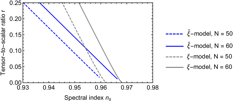
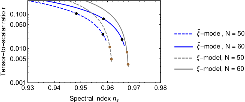
Figure 1: In the both figures, blue and gray lines show the cosmological observables $n_{s}$ and $r$ for the inflation model defined by Eqs. (4.50)-(4.55) (dubbed as $\tilde{\xi}$-model) and that defined by Eqs. (4.9) and (4.15) (dubbed as $\xi$-model), respectively. Solid (dashed) lines correspond to the predictions for $N=60\,(50)$. The black (brown) dots on each line in the bottom panel correspond to $\tilde{\xi}$ ($\xi$) $=0.1$ and $1$ from top to bottom.

In appendix B, we show that Eqs. (4.50)-(4.55) are compatible with the assumption that $S$ and the imaginary part of $\phi$ are stabilized at the origin during inflation, if we introduce an appropriate higher order term of $S$ in the frame function.

We note that the potential (4.48) does not exhibit runaway behavior in contrast to a naive non-holomorphic extension of the CSS models discussed in Sec. 3.2. The inflaton field rolls towards $\varphi\to 0$, and we expect that inflation ends at a point when the slow-roll condition is violated.

There are some remarks on the difference in comparison with the FKLMP model. First, although $\Phi$ is quadratic in $\varphi$, the Kähler potential has a non-trivial structure due to the existence of non-holomorphic terms, and the additional factor $V_{0}\propto\tilde{\xi}^{-m}$ is multiplied in the scalar potential. Because of this factor, the amplitude of the curvature perturbation is suppressed as $\mathcal{P}_{\zeta}\propto\tilde{\xi}^{-5+3/\tilde{\xi}}$, which may be fitted to the observational result $\mathcal{P}_{\zeta}\simeq\mathcal{O}(10^{-10})$ for $\tilde{\xi}\simeq\mathcal{O}(10^{2})$ and $\lambda\simeq\mathcal{O}(1)$. On the other hand, the prediction of the FKLMP model reads $\mathcal{P}_{\zeta}\propto\xi^{-2}$, which requires the value of $\xi$ as large as $\mathcal{O}(10^{5})$ provided that $\lambda\simeq\mathcal{O}(1)$. If we require that $m$ should be positive integer, $\tilde{\xi}$ is uniquely determined to be either $1$ or $3$, which leads to $m=8$ or $6$, respectively. In this case, $\tilde{\xi}$ is of the order of unity though $\lambda$ must be $\mathcal{O}(10^{-5})$. Second, the power law superpotential $W\propto S\phi^{m}$ is required in order to compensate the non-trivial $\varphi$ dependence of $V_{E}$ arising from the Kähler potential. In general, the power $m$ is not integer number. Finally, both in the FKLMP model and in this model, the prediction for the tensor-to-scalar ratio has a lower limit, but there is a difference in its value. In the FKLMP model the lower limit reads $r\gtrsim 12/N^{2}$ for $\xi\gg 1$, while in the above model the lower limit reads $r\gtrsim 48/N^{2}$ for $\tilde{\xi}\gg 1$.

4.4 Relation to kinetic formulation in the Einstein frame

In this subsection, we clarify the origin of differences or similarities of the models considered in this paper, and discuss their relation to the models constructed in the Einstein frame. First, we review the difference between the FKLMP model and the models constructed in the previous subsection by the use of the variable $\rho$ introduced in Sec. 4.1. After that, we highlight the relation to the models based on Einstein frame supergravity, taking the $\alpha$-attractor models for specific examples.

The difference in the lower limit on the tensor-to-scalar ratio between two models shown in the previous subsections originates from the difference in the coefficient $a_{2}$ of the leading pole in the kinetic term in the Einstein frame [see Eq. (4.7)]. To see the appearance of such a difference, let us take a closer look at the structure of the kinetic term of the inflaton field. From Eqs. (2.12) and (4.27), we can rewrite the kinetic term of the inflaton field in the Einstein frame in terms of the conformal factor $\Omega^{2}$,

$$\frac{\mathcal{L}_{{\rm kin},E}}{\sqrt{-g_{E}}}=-\frac{1}{2}\left(\frac{1}{\Omega^{2}}+\frac{6(\Omega^{\prime})^{2}}{\Omega^{2}}\right)(\partial\varphi)^{2}.$$ (4.57)

Then, if we adopt the following relation between $\rho$ and $\varphi$,

$$\rho\propto\Omega^{-\frac{2}{q}},$$ (4.58)

where $q$ is some real constant, the kinetic term reduces to

$$\frac{\mathcal{L}_{{\rm kin},E}}{\sqrt{-g_{E}}}=-\frac{1}{2}\left(\frac{q^{2}}{4(\Omega^{\prime})^{2}}+\frac{3q^{2}}{2}\right)\frac{(\partial\rho)^{2}}{\rho^{2}}.$$ (4.59)

If $\Omega^{\prime}$ remains constant, we can regard the coefficient of $(\partial\rho)^{2}/\rho^{2}$ in the above equation as a constant $a_{2}$. Hence, from Eq. (4.7) we estimate the prediction for the tensor-to-scalar ratio as

$$r=\frac{8a_{2}}{N^{2}}=\frac{8}{N^{2}}\left(\frac{q^{2}}{4(\Omega^{\prime})^{2}}+\frac{3q^{2}}{2}\right).$$ (4.60)

It is straightforward to check that the conformal factor $\Omega^{2}$ satisfying the condition $\Omega^{\prime}=\mathrm{const}.$ should be a quadratic function of $\varphi$, and that both the FKLMP model and the $\tilde{\xi}$-model in Sec. 4.3 satisfy this condition.

If $(\Omega^{\prime})^{2}>0$, the lower limit on $a_{2}$ is fixed by the second term $3q^{2}/2$, which does not depend on the parameters such as $\xi$ and $\tilde{\xi}$, but on the value of $q$. For instance, we have $q=1$ and $a_{2}>3/2$ in the FKLMP model, while $q=2$ and $a_{2}>6$ in the $\tilde{\xi}$-model. This fact results in the different lower limit on the tensor-to-scalar ratio $r\gtrsim 48/N^{2}$ in the $\tilde{\xi}$-model, which is four times larger than that in the FKLMP model.

We note that the validity of the choice in Eq. (4.58) depends on the form of the scalar potential in the Jordan frame. Namely, we must guarantee that the function $f(\phi)$ is chosen such that the scalar potential in the Einstein frame takes the form (4.30) with $\rho$ given by Eq. (4.58). In general, we can construct the desired form of $V_{E}(\rho)$ for $\rho=\Omega^{-2/q}$ with an arbitrary value of $q$ by choosing the scalar potential in the Jordan frame such that

$$V_{J}(\varphi)=\Omega(\varphi)^{4}V_{E}(\rho)\quad\text{with}\quad\rho=\Omega(\varphi)^{-\frac{2}{q}}.$$ (4.61)

The above equation explicitly shows that the choice of $V_{J}(\varphi)$ [or the choice of the function $f(\phi)$] depends on the value of $q$. In other words, it is possible to construct a set of models that give rise to the same form of $V_{E}(\rho)$ but have different values of $q$ (or different lower limits on $r$) by adjusting the scalar potential appropriately in the Jordan frame.

The above discussion does not imply that the $\tilde{\xi}$-model constructed in the previous subsection is equivalent to the FKLMP model except for the value of $q$. This is because the kinetic term and the scalar potential of these models are not exactly the same in the Einstein frame although they are the same at leading order in $\rho$. More specifically, we have

$$K_{E}(\rho)=\left[\frac{1}{4\xi(1-\rho)}+\frac{3}{2}\right]\frac{1}{\rho^{2}},\quad V_{E}(\rho)\propto(1-\rho)^{2},$$ (4.62)

for the FKLMP model with $\rho=\Omega^{-2}$, and

$$K_{E}(\rho)=\left[\frac{3}{\tilde{\xi}}+6\right]\frac{1}{\rho^{2}},\quad V_{E}(\rho)\propto(1-\rho)^{2m},$$ (4.63)

for the $\tilde{\xi}$-model with $\rho=\Omega^{-1}$. The difference in the subleading terms leads to the different predictions for $n_{s}$ and $r$ as shown in Fig. 1. However, by adjusting the scalar potential in the Jordan frame we can also construct a model that would lead to completely the same predictions except for the lower limit on $r$. For instance, it is possible to construct a variant of the $\tilde{\xi}$-model that would exhibit $q=1$ rather than $q=2$ by adjusting $f(\phi)$ according to Eq. (4.61). In such a case, $f(\phi)$ must be different from the monomial function $f=\lambda\phi^{m}$ specified in the previous subsection.

Next, let us consider the relation between the models constructed in the Jordan frame and those constructed in the Einstein frame, particularly the $\alpha$-attractor models.

We can show that the Kähler potential of the $\tilde{\xi}$-model [Eq. (4.50)] reduces to the following form (up to constant terms),

$$\mathcal{K}=-3\alpha\log(T+\bar{T}),$$ (4.64)

if we identify

$$T =1+\sqrt{\frac{2\tilde{\xi}}{3}}\phi,$$ (4.65)

$$\alpha =4\left(1+\frac{1}{2\tilde{\xi}}\right).$$ (4.66)

Equation (4.64) corresponds to the Kähler potential for the $\alpha$-attractor models with half-plane valuables $T$ and $\bar{T}$ [42, 43]. In such models, the parameter $\alpha$ is interpreted as the scalar curvature of the Kähler manifold,

$$\mathcal{R}_{K}=-g_{T\bar{T}}^{-1}\partial_{T}\partial_{\bar{T}}\log g_{T\bar{T}}=-\frac{2}{3\alpha}.$$ (4.67)

In the $\alpha$-attractor models defined in the Einstein frame, we can deduce the condition $\alpha>0$ from the requirement that the kinetic term in the Einstein frame must have the proper sign. Since the prediction for the tensor-to-scalar ratio is given by $r=12\alpha/N^{2}$ [9, 10], this fact implies that there is no lower limit on $r$ in the $\alpha$-attractor models. On the other hand, in the $\tilde{\xi}$-model defined in the Jordan frame, the lower limit on $\alpha$ in Eq. (4.66) becomes $\alpha>4$ as long as we require that $\tilde{\xi}$ should be real and positive.

It may appear surprising that two models (the $\tilde{\xi}$-model and the $\alpha$-attractor model) that have exactly the same structure in the Kähler potential lead to different lower limits on the parameter $\alpha$ (or on the tensor-to-scalar ratio). This difference arises from a peculiar feature of the Jordan frame. If we formally allow negative values of $\tilde{\xi}$ in Eq. (4.66), there would be no lower limit on $\alpha$ except for the condition $\alpha>0$ due to the requirement of the positive kinetic energy in the Einstein frame. However, the conformal factor in Eq. (4.40), $\Omega^{2}=(1+(\tilde{\xi}/3)^{1/2}\varphi)^{2}$, becomes complex for $\tilde{\xi}<0$, which leads to the ill-defined relation between the Jordan frame and the Einstein frame. Note that it is also possible to check this fact by using Eq. (4.59). Substituting $\Omega^{2}=(1+(\tilde{\xi}/3)^{1/2}\varphi)^{2}$ and $q=2$ into Eq. (4.59), we have

$$\frac{\mathcal{L}_{{\rm kin},E}}{\sqrt{-g_{E}}}=-\frac{1}{2}\left(\frac{3}{\tilde{\xi}}+6\right)\frac{(\partial\rho)^{2}}{\rho^{2}}.$$

Then, we see that there would be no lower limit on $a_{2}$ if we allow $\tilde{\xi}<0$. This corresponds to the case with $(\Omega^{\prime})^{2}<0$, which is incompatible with our assumption.

Unlike the $\tilde{\xi}$-model, the Kähler potential of the FKLMP model is not equivalent to that of the $\alpha$-attractor models, but the peculiarity of the Jordan frame mentioned above is also relevant to the FKLMP model. In this case, the conformal factor is given by $\Omega^{2}=1+\xi\varphi^{2}$. Substituting it and $q=1$ into Eq. (4.59), we have $a_{2}\to(4\xi)^{-1}+3/2$ in the large field limit. Then, if we formally allow negative values of $\xi$, there would be no lower limit on $a_{2}$. Such a regime is forbidden since $\Omega^{2}$ vanishes for a finite value of $\varphi$, and we cannot define the appropriate conformal transformation.

To recap the above discussions, the $\tilde{\xi}$-model constructed in the previous subsection is inequivalent to the FKLMP model in the sense that behaviors in the Einstein frame are not exactly the same, while in general it is possible to construct plural models in the Jordan frame that lead to the same dynamics in the Einstein frame by adjusting the scalar potential in the Jordan frame appropriately. For such models, there exists a finite lower limit on the tensor-to-scalar ratio due to the restriction that the conformal factor must be real and positive. Furthermore, the value of the lower limit is determined by the choice of the relation between $\rho$ and $\varphi$ [such as Eq. (4.58)], which originates from the choice of the scalar potential in the Jordan frame.

5 Summary and discussions

In this paper, we have discussed inflation models in Jordan frame supergravity. First of all, we have explicitly shown that the model proposed by Ferrara et al. is uniquely characterized by the following two requirements: (1) The kinetic terms of scalar fields should be canonical in the Jordan frame. (2) The frame function consists only of a holomorphic term (and its anti-holomorphic counterpart) for symmetry breaking terms. Then, we tried to relax the latter condition with keeping the former condition. In order to realize concrete examples of inflation models with asymptotically flat potential in this context, we introduced pole inflation technique and a stabilizer field. By imposing the canonical kinetic terms and pole structure, we have derived the condition for the frame function, whose solution yields a suitable example for inflation in Jordan frame supergravity. It should be noticed that pole structure does not necessarily guarantee potential suitable for inflation because it just guarantees asymptotic flatness of the potential and the potential can be runaway type and/or have a bump, which prevents the inflation from ending. We have confirmed that our model can certainly realize inflation with the help of the stabilizer field. It is quite interesting to embed the Higgs field and/or some fields beyond the Standard Model of particle physics to our models, which is left for future work.

The model explored in Sec. 4.3 predicts that there is a lower limit on the tensor-to-scalar ratio, $r\gtrsim 0.013$. We emphasize that the precise value of this limit is model-dependent, and closely related to the choice of the scalar potential in the Jordan frame, as shown in Sec. 4.4. It is notable that, if the predicted value of $r$ is sufficiently large, it is potentially accessible in future CMB $B$-mode experiments. Currently, the Planck collaboration has obtained a bound $r<0.10$ (95% CL, Planck TT+lowP) at the scale $k=0.002\,\mathrm{Mpc}^{-1}$ [4], and it is expected that the sensitivity on $r$ will be considerably improved in future ground-, balloon-, and space-based experiments [44]. Such future experimental studies will test the model discussed in this paper.

We have explicitly shown that the Kähler potential of the $\tilde{\xi}$-model in Sec. 4.3 is equivalent to that of the $\alpha$-attractor models, but there exists a non-trivial lower limit on the $\alpha$ parameter. This fact originates from the peculiar feature of the Jordan frame that the conformal factor must be real and positive such that we can define the appropriate conformal transformation between the Jordan frame and the Einstein frame. The choice of the frame function and the scalar potential in the Jordan frame can constrain the parameter space of the equivalent model in the Einstein frame, which leads to different predictions for the lower limit on the tensor-to-scalar ratio.

We emphasize that the model constructed in Sec. 4.3 is just one specific example, in which three guiding principles enumerated in Sec. 4.2 are satisfied. This fact does not exclude the possibility of obtaining other models that lead to pole inflation with the scalar fields having canonical kinetic terms in the Jordan frame. It would be interesting to extend our analysis to explore such inflationary models in a generic manner.

In addition to the inflation model with the quadratic frame function obtained in Sec. 4.3, we also found that naive non-holomorphic extensions of the CSS models with single power law functions lead to the scalar potential exhibiting runaway behavior, which is not suitable for describing inflation (see Sec. 3.2 and Appendix A). However, it can be used to construct a model that accounts for the accelerated expansion of the present Universe (see Ref. [45] for example), though freezing model is now less favored observationally. Here, the challenge is to construct the model compatible with the low energy supersymmetry breaking, which deserves further investigation.

Appendix A Non-holomorphic $\Delta$-deformed CSS models

In this appendix, we consider a non-holomorphic deformation of the CSS models discussed in Sec. 3.2. Here we adopt the following Kähler potential and frame function

$$\mathcal{K} =-3\log\left(-\frac{1}{3}\frac{\Phi}{Y}\right),$$ (A.1)

$$\Phi =-3+\delta_{\alpha\bar{\beta}}z^{\alpha}\bar{z}^{\bar{\beta}}+\Delta_{1}\mathcal{G}(z,\bar{z}),$$ (A.2)

$$Y =1+\Delta_{2}\mathcal{Y}(z,\bar{z}),$$ (A.3)

where $\mathcal{G}$ and $\mathcal{Y}$ are non-holomorphic functions, and $\Delta_{1}$ and $\Delta_{2}$ are some real constant parameters. From Eqs. (2.25) and (2.27), the kinetic terms in the Jordan frame read

$$\frac{\mathcal{L}_{{\rm kin},J}}{\sqrt{-g_{J}}}=-\left[\delta_{\alpha\bar{\beta}}+\Delta_{1}\mathcal{G}_{\alpha\bar{\beta}}+\Delta_{2}\frac{\Phi}{Y^{2}}\left(\Delta_{2}\mathcal{Y}_{\alpha}\mathcal{Y}_{\bar{\beta}}-Y\mathcal{Y}_{\alpha\bar{\beta}}\right)\right]g_{J}^{\mu\nu}\hat{\partial}_{\mu}z^{\alpha}\hat{\partial}_{\nu}\bar{z}^{\bar{\beta}},$$ (A.4)

where the subscripts $\alpha$ and $\bar{\beta}$ represent a derivative with respect to $z^{\alpha}$ and $\bar{z}^{\bar{\beta}}$, respectively. If we take $\Delta_{1}=\Delta_{2}=0$, the kinetic terms in the Jordan frame are canonically normalized, and the CSS models are recovered.

Hereafter, we focus on the models with two real scalar fields $\phi$ and $S$ with the superpotential given by Eq. (4.20). If we further assume that $S$ is stabilized at $S=0$ and that derivatives of $\mathcal{G}$ and $\mathcal{Y}$ with respect to $S$ and $\bar{S}$ vanish at that point, we can still use Eqs. (4.21) and (4.22), and the scalar potential in the Einstein frame is given by

$$V_{E}=\frac{9Y^{3}}{\Phi^{2}}\left|f\right|^{2}=\frac{(1+\Delta_{2}\mathcal{Y})^{3}}{(1-\frac{1}{3}|\phi|^{2}-\frac{\Delta_{1}}{3}\mathcal{G})^{2}}\left|f\right|^{2}.$$ (A.5)

Let us assume that $f$, $\mathcal{G}$, and $\mathcal{Y}$ are given by single power law functions of $\phi$ at $S=0$,

$$f(\phi)=\lambda\phi^{l},\quad\mathcal{G}(\phi,\bar{\phi})=|\phi|^{2m},\quad\text{and}\quad\mathcal{Y}(\phi,\bar{\phi})=|\phi|^{2n},$$ (A.6)

where $l$, $m$, and $n$ are positive integers, and $\lambda$ is a complex parameter. Then, the scalar potential becomes a function of the radial direction $\varphi\equiv|\phi|/\sqrt{2}$,

$$V_{E}=\frac{|\lambda|^{2}}{2^{l}}\frac{\left(1+\frac{\Delta_{2}}{2^{n}}\varphi^{2n}\right)^{3}}{(1-\frac{1}{6}\varphi^{2}-\frac{1}{3}\frac{\Delta_{1}}{2^{m}}\varphi^{2m})^{2}}\varphi^{2l}.$$ (A.7)

In particular, it approaches to a constant value in the large field limit if $l=2m-3n$, which appears to be suitable for inflation. However, in such cases the potential exhibits runaway behavior, as shown below.

In order to see the behavior of the scalar potential in the large field limit, we differentiate Eq. (A.7) with respect to $\varphi$ and impose the condition $l=2m-3n$,

$$\frac{\partial V_{E}}{\partial\varphi} =\left[2m-3n+\frac{1}{6}(2-2m+3n)\varphi^{2}+\frac{n\Delta_{1}}{2^{m}}\varphi^{2m}+\left(2m+\frac{1-m}{3}\varphi^{2}\right)\frac{\Delta_{2}}{2^{n}}\varphi^{2n}\right]$$

$$\quad\times\frac{2V_{E}}{\varphi\left(1+\frac{\Delta_{2}}{2^{n}}\varphi^{2n}\right)\left(1-\frac{1}{6}\varphi^{2}-\frac{1}{3}\frac{\Delta_{1}}{2^{m}}\varphi^{2m}\right)}.$$ (A.8)

We also note that $\Delta_{1}<0$ and $\Delta_{2}>0$ are required, since otherwise we have $\Phi=0$ or $Y=0$ for a finite value of $\varphi$, which leads to a singularity in the scalar potential or in the kinetic term, and prevent $\varphi$ from rolling down to a small field value $\varphi\ll 1$ after inflation. With these preliminaries, we can consider two different cases according to the value of $m$. If $m>1$, the term with the highest power in the bracket in the first line of Eq. (A.8) is $n\Delta_{1}|\phi|^{2m}$ or $(1-m)\Delta_{2}|\phi|^{2n+2}/3$, and both of them are negative, since we assume that $\Delta_{1}<0$ and $\Delta_{2}>0$. Furthermore, the denominator of the second line of Eq. (A.8) approaches to $-\sqrt{2}\Delta_{1}\Delta_{2}|\phi|^{2(n+m)+1}/3$ in the large field limit, and it is positive. Therefore, $\partial V_{E}/\partial\varphi$ becomes negative in the large field limit, which implies that the potential exhibits runaway behavior for $m>1$. On the other hand, if $m=1$, which is only possible for $l=2$ and $n=0$ since we assume that $l=2m-3n$ and that $l$, $m$, $n$ are positive integers, Eq. (A.8) reduces to

$$\frac{\partial V_{E}}{\partial\varphi}=\frac{4V_{E}}{\varphi\left(1-\frac{1}{6}(1+\Delta_{1})\varphi^{2}\right)}.$$

This becomes positive for $\Delta_{1}<-1$, but in such a case the kinetic term in the Einstein frame has a wrong sign, $g_{\phi\bar{\phi}}=(1+\Delta_{1})/(1-\frac{1}{6}(1+\Delta_{1})\varphi^{2})^{2}<0$. From these facts, we conclude that the potential (A.7) always exhibits runaway behavior in the large field limit when $l=2m-3n$.

Appendix B Stabilization of non-inflaton fields

In this appendix, we show that the Kähler potential, frame function, and superpotential given by Eqs. (4.50)-(4.55) are compatible with the assumption that ${\rm Im}(\phi)=0$ and $S=0$ during inflation if we introduce $S$-dependence in the frame function and the Kähler potential appropriately.

For simplicity, we assume that the frame function and the Kähler potential depend only on $|S|^{2}$, not on $S^{2}$ or $\bar{S}^{2}$, and that the function $Y$ is independent of $|S|^{2}$. Therefore, we use the same expression for $Y$ as in Eq. (4.44), which is rewritten in terms of $\phi$ and $\bar{\phi}$ as

$$\log Y=-2\left(1+{1\over\tilde{\xi}}\right)\log\left(1+\sqrt{{\tilde{\xi}\over 6}}(\phi+\bar{\phi})\right)\,.$$ (B.1)

On the other hand, we consider the following frame function,

$$\Phi=\mathrm{e}^{F(|S|^{4})}\left[-3\left(1+\sqrt{\tilde{\xi}\over 6}(\phi+\bar{\phi})\right)^{2}+|S|^{2}\right]\,,$$ (B.2)

where $F(|S|^{4})$ is introduced in order to guarantee the stabilization of $S$, and it is a function of $|S|^{4}$ satisfying $F\rightarrow 0$ for $S\rightarrow 0$. This frame function and the function (B.1) satisfy the conditions for which the kinetic terms of $\phi$ and $S$ become canonical,

$$\left(\log Y\right)_{\alpha\bar{\beta}}={\Phi_{\alpha\bar{\beta}}-\delta_{\alpha\bar{\beta}}\over\Phi}\,,$$ (B.3)

when $S=0$. From Eqs. (B.1) and (B.2), the Kähler potential can be written as

$$\mathcal{K}=-3\log\left[\left(1+\sqrt{\tilde{\xi}\over 6}(\phi+\bar{\phi})\right)^{2}-{1\over 3}|S|^{2}\right]-6\left(1+{1\over\tilde{\xi}}\right)\log\left(1+\sqrt{{\tilde{\xi}\over 6}}(\phi+\bar{\phi})\right)-3F(|S|^{4})\,.$$ (B.4)

Using the frame function (B.2) and the Kähler potential (B.4), we calculate the effective mass for ${\rm Im}(\phi)$ and $S$:

$$m^{2}_{{\rm Im}(\phi)}\equiv{1\over 2}\mathcal{K}_{\phi\bar{\phi}}^{-1}\left.{\partial^{2}V_{E}\over\partial\left({\rm Im}(\phi)\right)^{2}}\right|_{{\rm Im}(\phi)=S=0}\,,$$ (B.5)

$$m^{2}_{S}\equiv\mathcal{K}_{S\bar{S}}^{-1}\left.{\partial^{2}V_{E}\over\partial s^{2}}\right|_{{\rm Im}(\phi)=S=0}\,,$$ (B.6)

where $s=\sqrt{2}|S|$. Because the frame function and the Kähler potential depend only on $|S|^{2}$, the mass for ${\rm Re}(S)$ and ${\rm Im}(S)$ are equivalent, which can be easily confirmed from the detailed calculation that we will show in the following.

In order to compute the masses (B.5) and (B.6), we need to compute $\mathcal{K}_{\alpha}$ and $\mathcal{K}_{\alpha\bar{\beta}}$. The first derivatives of the Kähler potential become

$$\partial_{\phi}\mathcal{K}=\partial_{\bar{\phi}}\mathcal{K}=-\sqrt{{6\over\tilde{\xi}}}{1+2\tilde{\xi}\over 1+\sqrt{{\tilde{\xi}\over 6}}(\phi+\bar{\phi})}+\mathcal{O}(S^{2})\,,$$ (B.7)

$$\partial_{S}\mathcal{K}=\overline{\partial_{\bar{S}}\mathcal{K}}=\bar{S}\left(1+\sqrt{{\tilde{\xi}\over 6}}(\phi+\bar{\phi})\right)^{-2}+\mathcal{O}(S^{3})\,.$$ (B.8)

The second derivatives of the Kähler potential are given as

$$\partial_{\phi}\partial_{\bar{\phi}}\mathcal{K}=(1+2\tilde{\xi})\left(1+\sqrt{{\tilde{\xi}\over 6}}(\phi+\bar{\phi})\right)^{-2}+\tilde{\xi}\left(1+\sqrt{{\tilde{\xi}\over 6}}(\phi+\bar{\phi})\right)^{-4}|S|^{2}+\mathcal{O}(S^{3})\,,$$ (B.9)

$$\partial_{S}\partial_{\bar{\phi}}\mathcal{K}=\overline{\partial_{\phi}\partial_{\bar{S}}\mathcal{K}}=-2\sqrt{{\tilde{\xi}\over 6}}\left(1+\sqrt{{\tilde{\xi}\over 6}}(\phi+\bar{\phi})\right)^{-3}\bar{S}+\mathcal{O}(S^{3})\,,$$ (B.10)

$$\partial_{S}\partial_{\bar{S}}\mathcal{K}=\left(1+\sqrt{{\tilde{\xi}\over 6}}(\phi+\bar{\phi})\right)^{-2}+{2\over 3}\left(1+\sqrt{{\tilde{\xi}\over 6}}(\phi+\bar{\phi})\right)^{-4}|S|^{2}-3F_{S\bar{S}}+\mathcal{O}(S^{3})\,,$$ (B.11)

where $F_{S\bar{S}}=\partial_{S}\partial_{\bar{S}}F$. Therefore, $g^{\alpha\bar{\beta}}$ become

$$g^{\phi\bar{\phi}}={1\over 1+2\tilde{\xi}}\left(1+\sqrt{{\tilde{\xi}\over 6}}(\phi+\bar{\phi})\right)^{2}+\mathcal{O}(S^{2})\,,$$ (B.12)

$$g^{\phi\bar{S}}=\overline{g^{S\bar{\phi}}}={2\sqrt{{\tilde{\xi}\over 6}}\over 1+2\tilde{\xi}}\left(1+\sqrt{{\tilde{\xi}\over 6}}(\phi+\bar{\phi})\right)\bar{S}+\mathcal{O}(S^{3})\,,$$ (B.13)

$$g^{S\bar{S}}=\left(1+\sqrt{{\tilde{\xi}\over 6}}(\phi+\bar{\phi})\right)^{2}+\left[{3F_{S\bar{S}}\over|S|^{2}}\left(1+\sqrt{{\tilde{\xi}\over 6}}(\phi+\bar{\phi})\right)^{4}-{2(1+\tilde{\xi})\over 3(1+2\tilde{\xi})}\right]|S|^{2}+\mathcal{O}(S^{3})\,.$$ (B.14)

$V_{E}$ is given as

$$V_{E} ={\mathrm{e}}^{\mathcal{K}}\left(g^{\alpha\bar{\beta}}\nabla_{\alpha}W\nabla_{\bar{\beta}}\bar{W}-3|W|^{2}\right)$$

$$=|\lambda|^{2}|\phi|^{2m}\left(1+\sqrt{{\tilde{\xi}\over 6}}(\phi+\bar{\phi})\right)^{-2m}+|\lambda|^{2}|S|^{2}|\phi|^{2(m-1)}\left(1+\sqrt{{\tilde{\xi}\over 6}}(\phi+\bar{\phi})\right)^{-2(m+1)}$$

$$\qquad\times\left[2\left({2+5\tilde{\xi}\over 3(1+2\tilde{\xi})}+{3\over\tilde{\xi}}+3+{3F_{S\bar{S}}\over 2|S|^{2}}\left(1+\sqrt{{\tilde{\xi}\over 6}}(\phi+\bar{\phi})\right)^{4}\right)|\phi|^{2}+{m^{2}\over 1+2\tilde{\xi}}\left(1-{\tilde{\xi}\over 6}(\phi+\bar{\phi})^{2}\right)\right]\,,$$ (B.15)

up to $\mathcal{O}(|S|^{2})$. Setting $\phi=\bar{\phi}=\varphi/\sqrt{2}$ and $S=0$, we have

$$V_{E}=|\lambda|^{2}\left(\frac{\frac{\varphi}{\sqrt{2}}}{1+\sqrt{\frac{\tilde{\xi}}{3}}\varphi}\right)^{2m}.$$ (B.16)

Therefore, the Hubble parameter during inflation in the large field limit $\varphi\gg\sqrt{3/\tilde{\xi}}$ reads

$$H_{\rm inf}^{2}=\frac{V_{E}}{3}\simeq\left(\frac{3}{2\tilde{\xi}}\right)^{m}\frac{|\lambda|^{2}}{3}.$$ (B.17)

From Eqs. (B.5), (B.9), and (B.15), we obtain

$$m^{2}_{{\rm Im}(\phi)}=\frac{2m}{1+2\tilde{\xi}}\frac{|\lambda|^{2}}{2^{m}}\frac{\varphi^{2(m-1)}}{\left(1+\sqrt{\frac{\tilde{\xi}}{3}}\varphi\right)^{2(m-1)}}\\ \simeq\frac{2(5\tilde{\xi}+3)}{1+2\tilde{\xi}}H_{\rm inf}^{2}\,,$$ (B.18)

where we take the large field limit in the last equality. In this limit, $m^{2}_{{\rm Im}(\phi)}$ is larger than $H_{\rm inf}^{2}$ for $\tilde{\xi}>-5/8$. Therefore, we confirm that the imaginary part of $\phi$ is stabilized at the origin during inflation.

Setting $F(|S|^{4})=\zeta|S|^{4}/4$ and $\phi=\bar{\phi}=\varphi/\sqrt{2}$ in Eq. (B.15), we have

$$V_{E} ={|\lambda|^{2}\over 2^{m}}\varphi^{2m}\left(1+\sqrt{{\tilde{\xi}\over 3}}\varphi\right)^{-2m}+{|\lambda|^{2}\over 2^{m-1}}|S|^{2}\varphi^{2(m-1)}\left(1+\sqrt{{\tilde{\xi}\over 3}}\varphi\right)^{-2(m+1)}$$

$$\qquad\times\left[\left({2+5\tilde{\xi}\over 3(1+2\tilde{\xi})}+{3\over\tilde{\xi}}+3+{3\zeta\over 2}\left(1+\sqrt{{\tilde{\xi}\over 3}}\varphi\right)^{4}\right)\varphi^{2}+{m^{2}\over 1+2\tilde{\xi}}\left(1-{\tilde{\xi}\over 3}\varphi^{2}\right)\right]\,.$$ (B.19)

Then, $m_{S}^{2}$ becomes

$$m_{S}^{2}={|\lambda|^{2}\over 2^{m}}\varphi^{2(m-1)}\left(1+\sqrt{{\tilde{\xi}\over 3}}\varphi\right)^{-2m}\left[\left(-{1\over 3}+{3\zeta\over 2}\left(1+\sqrt{{\tilde{\xi}\over 3}}\varphi\right)^{4}\right)\varphi^{2}+{m^{2}\over 1+2\tilde{\xi}}\right]\,,$$ (B.20)

where we used $m=5+3/\tilde{\xi}$. This clarifies that $m_{S}^{2}$ inevitably becomes negative for large $\varphi$ when $\zeta=0$ (or $F=0$). When $\zeta\neq 0$, the ratio between $m_{S}^{2}$ and $H_{\rm inf}^{2}$ becomes

$${m_{S}^{2}\over H_{\rm inf}^{2}}\sim\zeta\tilde{\xi}^{2}\varphi^{4}\,,$$ (B.21)

for large $\varphi$. Therefore, $S$ is sufficiently stabilized during inflation for positive $\zeta$.

References

- [1] C. L. Bennett et al. [WMAP Collaboration], Astrophys. J. Suppl. 208, 20 (2013) [arXiv:1212.5225 [astro-ph.CO]].
- [2] R. Adam et al. [Planck Collaboration], Astron. Astrophys. 594, A1 (2016) [arXiv:1502.01582 [astro-ph.CO]].
- [3] G. Hinshaw et al. [WMAP Collaboration], Astrophys. J. Suppl. 208, 19 (2013) [arXiv:1212.5226 [astro-ph.CO]].
- [4] P. A. R. Ade et al. [Planck Collaboration], Astron. Astrophys. 594, A20 (2016) [arXiv:1502.02114 [astro-ph.CO]].
- [5] A. A. Starobinsky, Phys. Lett. 91B, 99 (1980).
- [6] J. L. Cervantes-Cota and H. Dehnen, Nucl. Phys. B 442, 391 (1995) [astro-ph/9505069].
- [7] F. L. Bezrukov and M. Shaposhnikov, Phys. Lett. B 659, 703 (2008) [arXiv:0710.3755 [hep-th]].
- [8] S. Ferrara, R. Kallosh, A. Linde and M. Porrati, Phys. Rev. D 88, no. 8, 085038 (2013) [arXiv:1307.7696 [hep-th]].
- [9] R. Kallosh, A. Linde and D. Roest, JHEP 1311 (2013) 198 [arXiv:1311.0472 [hep-th]].
- [10] J. J. M. Carrasco, R. Kallosh and A. Linde, JHEP 1510, 147 (2015) [arXiv:1506.01708 [hep-th]].
- [11] C. Pallis, JCAP 1404, 024 (2014) [arXiv:1312.3623 [hep-ph]].
- [12] G. F. Giudice and H. M. Lee, Phys. Lett. B 733 (2014) 58 [arXiv:1402.2129 [hep-ph]].
- [13] C. Pallis, JCAP 1408, 057 (2014) [arXiv:1403.5486 [hep-ph]].
- [14] R. Kallosh, Phys. Rev. D 89, no. 8, 087703 (2014) [arXiv:1402.3286 [hep-th]].
- [15] M. Galante, R. Kallosh, A. Linde and D. Roest, Phys. Rev. Lett. 114, no. 14, 141302 (2015) [arXiv:1412.3797 [hep-th]].
- [16] B. J. Broy, M. Galante, D. Roest and A. Westphal, JHEP 1512, 149 (2015) [arXiv:1507.02277 [hep-th]].
- [17] T. Terada, Phys. Lett. B 760, 674 (2016) [arXiv:1602.07867 [hep-th]].
- [18] K. Nakayama, K. Saikawa, T. Terada and M. Yamaguchi, JHEP 1605, 067 (2016) [arXiv:1603.02557 [hep-th]].
- [19] T. Kobayashi, O. Seto and T. H. Tatsuishi, arXiv:1703.09960 [hep-th].
- [20] K. Maeda, Phys. Rev. D 39, 3159 (1989).
- [21] C. Armendariz-Picon, Phys. Rev. D 66, 064008 (2002) [astro-ph/0205187].
- [22] E. E. Flanagan, Class. Quant. Grav. 21, 3817 (2004) [gr-qc/0403063].
- [23] R. Catena, M. Pietroni and L. Scarabello, Phys. Rev. D 76, 084039 (2007) [astro-ph/0604492].
- [24] N. Deruelle and M. Sasaki, Springer Proc. Phys. 137, 247 (2011) [arXiv:1007.3563 [gr-qc]].
- [25] T. Chiba and M. Yamaguchi, JCAP 1310, 040 (2013) [arXiv:1308.1142 [gr-qc]].
- [26] A. Y. Kamenshchik and C. F. Steinwachs, Phys. Rev. D 91, no. 8, 084033 (2015) [arXiv:1408.5769 [gr-qc]].
- [27] T. Futamase and K. Maeda, Phys. Rev. D 39, 399 (1989).
- [28] R. Kallosh, L. Kofman, A. D. Linde and A. Van Proeyen, Class. Quant. Grav. 17, 4269 (2000) Erratum: [Class. Quant. Grav. 21, 5017 (2004)] [hep-th/0006179].
- [29] S. Ferrara, R. Kallosh, A. Linde, A. Marrani and A. Van Proeyen, Phys. Rev. D 82, 045003 (2010) [arXiv:1004.0712 [hep-th]].
- [30] S. Ferrara, R. Kallosh, A. Linde, A. Marrani and A. Van Proeyen, Phys. Rev. D 83, 025008 (2011) [arXiv:1008.2942 [hep-th]].
- [31] R. Kallosh and A. Linde, JCAP 1306, 027 (2013) [arXiv:1306.3211 [hep-th]].
- [32] D. Z. Freedman and A. Van Proeyen, “Supergravity,” Cambridge University Press, Cambridge U.K. (2012).
- [33] W. Buchmüller, V. Domcke and K. Schmitz, JCAP 1304, 019 (2013) [arXiv:1210.4105 [hep-ph]].
- [34] K. Das, V. Domcke and K. Dutta, JCAP 1703, no. 03, 036 (2017) [arXiv:1612.07075 [hep-ph]].
- [35] K. Nakayama and F. Takahashi, JCAP 1011, 039 (2010) [arXiv:1009.3399 [hep-ph]].
- [36] L. H. Ford, Phys. Rev. D 35, 2955 (1987).
- [37] P. J. E. Peebles and A. Vilenkin, Phys. Rev. D 59, 063505 (1999) [astro-ph/9810509].
- [38] G. N. Felder, L. Kofman and A. D. Linde, Phys. Rev. D 60, 103505 (1999) [hep-ph/9903350].
- [39] M. Kawasaki, M. Yamaguchi and T. Yanagida, Phys. Rev. Lett. 85, 3572 (2000) [hep-ph/0004243].
- [40] R. Kallosh, A. Linde and T. Rube, Phys. Rev. D 83, 043507 (2011) [arXiv:1011.5945 [hep-th]].
- [41] D. Roest, M. Scalisi and I. Zavala, JCAP 1311, 007 (2013) [arXiv:1307.4343 [hep-th]].
- [42] S. Cecotti and R. Kallosh, JHEP 1405, 114 (2014) [arXiv:1403.2932 [hep-th]].
- [43] R. Kallosh and A. Linde, Comptes Rendus Physique 16, 914 (2015) [arXiv:1503.06785 [hep-th]].
- [44] J. Errard, S. M. Feeney, H. V. Peiris and A. H. Jaffe, JCAP 1603, no. 03, 052 (2016) [arXiv:1509.06770 [astro-ph.CO]].
- [45] B. Ratra and P. J. E. Peebles, Phys. Rev. D 37, 3406 (1988).