Multi-technique investigation of the binary fraction among A-F type candidate hybrid variable stars discovered by Kepler

Abstract

Context. Hundreds of candidate hybrid pulsators of intermediate type A–F were revealed by the recent space missions. Hybrid pulsators allow to study the full stellar interiors, where both low-order p- and high-order g-modes are simultaneously excited. The true hybrid stars must be identified since other processes, related to stellar multiplicity or rotation, might explain the presence of (some) low frequencies observed in their periodograms.

Aims. We measured the radial velocities of 50 candidate $\delta$ Scuti - $\gamma$ Doradus hybrid stars from the Kepler mission with the Hermes and Ace spectrographs over a time span of months to years. We aim to derive the fraction of binary and multiple systems and to provide an independent and homogeneous determination of the atmospheric properties and $v\,\mathrm{sin}\,i$ for all targets. The long(er)-term objective is to identify the (probable) physical cause of the low frequencies.

Methods. We computed 1-D cross-correlation functions (CCFs) in order to find the best set of parameters in terms of the number of components, spectral type(s) and $v\,\mathrm{sin}\,i$ for each target. Radial velocities were measured from spectrum synthesis and by using a 2-D cross-correlation technique in the case of double- and triple-lined systems. Fundamental parameters were determined by fitting (composite) synthetic spectra to the normalised median spectra corrected for the appropriate Doppler shifts.

Results. We report on the analysis of 478 high-resolution Hermes and 41 Ace spectra of A/F-type candidate hybrid pulsators from the Kepler field. We determined their radial velocities, projected rotational velocities, atmospheric properties and classified our targets based on the shape of the CCFs and the temporal behaviour of the radial velocities. We derived orbital solutions for seven new systems. Three long-period preliminary orbital solutions are confirmed by a photometric time-delay analysis. Finally, we determined a global multiplicity fraction of 27% in our sample of candidate hybrid stars.

1 Introduction

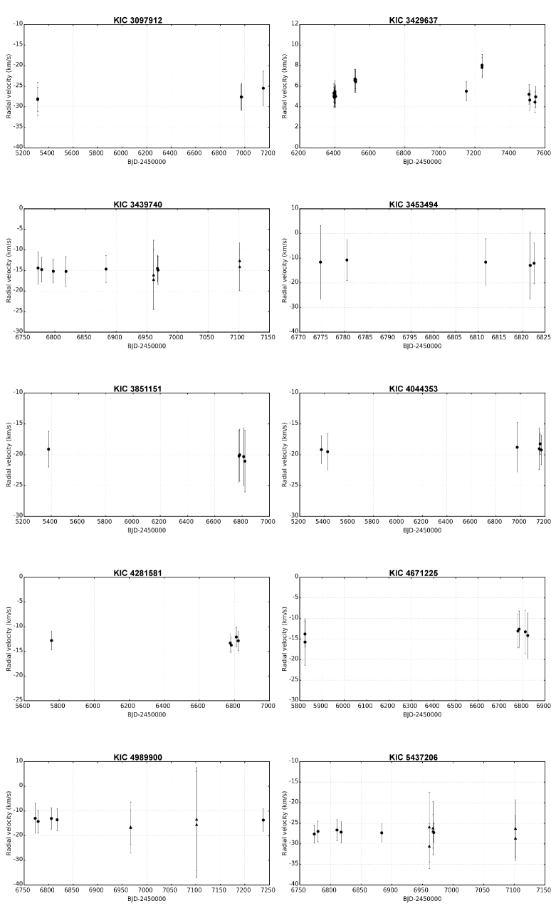
Figure 2: Radial velocity plots for 44 Kepler objects. The symbols indicate data collected with the Hermes ($\circ$, $\bullet$) or Ace spectrographs ($\bigtriangleup$).

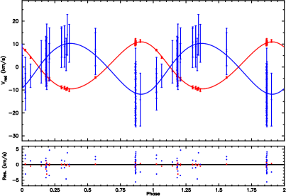
Figure 2: Radial velocities for the mass centre of the inner binary (AB) and for component C of KIC 4480321, plotted over a possible orbital solution with a period of 2280 days. The residuals are shown in the bottom part.

Many different physical processes compete in the outer atmospheres of A- and F-type main-sequence (MS) stars and their slightly more evolved cousins. In the corresponding region of the H-R diagram, we find the following important transitions:
- 1. the transition from average ”slow” to average ”fast” rotation. The distribution of $v\,\mathrm{sin}\,i$ as a function of spectral type shows that stars cooler than F5 have small $v\,\mathrm{sin}\,i$ (typically ¡ 10 km s^-1), whereas $v\,\mathrm{sin}\,i$ can reach several hundreds of km s^-1 for hotter stars (Royer 2009, cf. Fig. 2 from Royer et al. 2014);
- 2. the transition from deep to shallow convection, i.e. from convective to radiative envelopes. Theoretical models indicate a dramatic change in the structure of the outer envelopes near the red edge (RE) of the $\delta$ Sct instability strip, i.e. near $T_{\mathrm{eff}}$ = 7000 K (Christensen-Dalsgaard 2000). This transition (where the sudden onset of convection in the stellar envelope starts, see D’Antona et al. 2002) has also been described as a second ”Böhm-Vitense gap”;
- 3. the transition from mode driving by convective blocking near the base of the convective envelope (exciting gravity modes of type $\gamma$ Dor) (Dupret et al. 2004, 2005) to mode driving by the opacity mechanism (exciting acoustic modes of type $\delta$ Sct). Both instability strips are largely overlapping, which suggests that two regimes of modes could be simultaneously excited in some stars (i. e. the so-called “hybrid” stars). A recent study of a large sample of candidate $\gamma$ Dor stars suggests that the latter are confined to the $T_{\mathrm{eff}}$-range from 6900 to 7400 K on the MS, which corresponds to the region in the Hertzsprung-Russell diagram where $\gamma$ Dor pulsations are theoretically predicted (Tkachenko et al. 2013);
- 4. the transition from significant chromospheric activity and (coronal) X-ray emission to (almost) null emission. Such X-ray emission is expected for cool stars (type A7 and later) due to magnetic activity as well as for hot stars (type B2 and earlier) due to wind shocks. Intermediate spectral types are virtually X-ray dark (Schröder & Schmitt 2007; Robrade & Schmitt 2009). The former transition occurs abruptly, over a temperature interval no larger than 100 K in width, i.e. at approximately $T_{\mathrm{eff}}$ = 8250 $\pm$ 50 K (Simon et al. 2002). Within this narrow temperature range, chromospheric emission abruptly drops from solar brightness levels to more than one order of magnitude less. These phenomena are linked to the presence of surface convection zones and stellar magnetic fields, ultimately held responsible for the observed activity (Schröder & Schmitt 2007). Exceptions are the young Herbig Ae/Be stars and the peculiar Ap/Bp stars, where fossil magnetic fields are thought to play a role in the production of X-rays.
The origin of the stellar magnetic fields should also be considered. Dynamo processes generate fields in most of the low-mass stars of the MS, whereas the origin of the large-scale magnetic fields in massive stars is not yet understood (Fossati et al. 2015; Morel et al. 2015). On the other hand, magnetic fields are rare among the intermediate-mass stars. There is indeed no normal A star known with a fossil magnetic field of average strength (Aurière et al. 2007; Lignières et al. 2014) : either the fields are (very) strong (B_long ¿ 100 G) as in Ap stars (e.g. Mathys 2001), or ultra weak (B_long ¡ 1 G) as in Am stars (Blazère et al. 2014). Most chemically peculiar stars, however, appear to possess a magnetic field which brakes the rotation and stabilizes the atmosphere, enabling processes of atomic diffusion (Michaud et al. 2015).

In this complex region (see also Antoci 2014), a new group of pulsators has been revealed on the basis of the analysis of the Kepler light curves: they are called the $\delta$ Sct – $\gamma$ Dor or $\gamma$ Dor – $\delta$ Sct candidate hybrid stars (Grigahcène et al. 2010; Uytterhoeven et al. 2011). These candidate hybrid stars are A/F-type pulsating stars located across the instability strips of the $\delta$ Sct and the $\gamma$ Dor pulsators. Their light curves exhibit frequencies in both regimes. A first suspicion of the co-existence of both p- and g- modes already arose from a search for multiperiodicity in early A-type stars based on the Hipparcos epoch photometry (e. g. Koen 2001). Because the hotter ones are unexplained by theoretical models (Grigahcène et al. 2010; Balona et al. 2015), it is important to unravel the physical origin of their low frequencies and to confirm the cases of genuine hybrid pulsation. In the case of KIC 9533489, an object with $T_{\mathrm{eff}}$ of 7500 K, the authors concluded in favour of a true hybrid character of the oscillations (Bognár et al. 2015). It is furthermore critical to look for binarity in such stars. One reason is that some of the low frequencies should not be attributed to pulsation but perhaps to ellipsoidality and reflection or even something more exotic (like shallow eclipses or a heartbeat phenomenon). Another reason is that tidal forces in close companions may excite a number of g-modes (as harmonics of the orbital frequency) which would not be excited if the star was single. This could be the case of a pulsating star in an eccentric, close binary, where the dynamical tidal forces excite g-mode pulsations (Willems & Aerts 2002). Moreover, a normal $\gamma$ Dor star coupled to a normal $\delta$ Sct star will also mimic a $\gamma$ Dor – $\delta$ Sct hybrid.

The confirmation of genuine cases of hybrid pulsation thus represents an unavoidable step in the study of the A/F-type hybrid phenomenon. In this work, we aim to estimate the fraction of short-period (i.e. with orbital periods between about 1 and 50 d) spectroscopic systems among a sample of brighter A/F-type candidate hybrid stars discovered by the Kepler satellite. Some preliminary results have been reported by Lampens et al. (2015). This survey is based on the 171 candidate hybrid Kepler stars first studied by Uytterhoeven et al. (2011). The following definition of a hybrid star was used in their study:

• frequencies detected in the $\gamma$ Dor (i.e. ¡ 5 d^-1) and $\delta$ Sct (i.e. ¿ 5 d^-1) domains;

• the amplitudes in both domains are either comparable, or they do not differ by more than a factor of 5–7;

• at least two independent frequencies detected in both regimes with amplitudes higher than 100 ppm.
  

Section 2 describes the target selection, the observational strategy, the campaigns and the observations. Section 3 deals with the data processing. In Section 4, we explain the methodology and the data analysis. In Sections 5 and 7, the results of the classification and the orbital solutions of the newly discovered systems, respectively, are presented. The extraction of the physical parameters is discussed in Section 6. In Sect. 8, we study the periodograms based on the Kepler data and we present an observational H-R diagram in Sect. 9. A discussion and conclusions from this work are provided in Section 10.

2 Sample and observational strategy

We selected 50 of the brightest objects among the A/F-type candidate hybrid stars classified by Uytterhoeven et al. (2011, cf. Table 3). The observations were performed in the observing seasons from Aug. 2013 until Dec. 2016 with the high-resolution fibre-fed échelle spectrograph Hermes (High Efficiency and Resolution Mercator Echelle Spectrograph, Raskin et al. (2011)) mounted at the focus of the 1.2-m Mercator telescope located at the international observatory Roque de los Muchachos (ORM, La Palma, Spain). The instrument is operated by the University of Leuven under the supervision of the Hermes Consortium. It records the optical spectrum in the range $\lambda$ = 377 - 900 nm across 55 spectral orders in a single exposure. The resolving power in the high-resolution mode is R = 85 000. Advantages of the instrument are its broad spectral coverage, high stability (the velocity stability of a radial velocity standard star is about 50 m s^-1, priv. commun., IvS, Leuven) and excellent throughput (Raskin et al. 2011). Table 1 lists the journal of the spectroscopic campaigns.

More spectra were obtained with the new Ace fibre-fed échelle spectrograph attached to the 1-m RCC telescope of the Konkoly Observatory at Piszkés-tető, Hungary. The Ace spectrograph covers the 415 - 915 nm wavelength range with a resolution R = 20 000. A total of 41 Ace spectra was acquired for 11 targets during the winter of 2014-2015 (Table 1).

Table 1: Log of spectroscopic observations.

Range of JDs	Range of dates	Nr of spectra
From - to	From - to
$24[55198-56293]$	Jan, 2010 - Dec, 2012	62
$24[56513-56607]$	Aug 08 - Nov 10, 2013	64
$24[56772-56974]$	Apr 24 - Nov 12, 2014	188
$24[56932-57097]$	Oct 01 - Mar 15, 2014-15	41
$24[57150-57324]$	May 07 - Oct 28, 2015	105
$24[57466-57739]$	Mar 18 - Dec 16, 2016	59

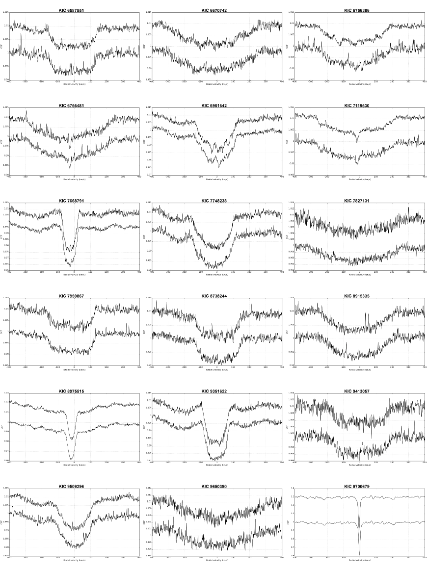
Figure 1: Cross-correlation functions for 48 Kepler objects (cont’ed).

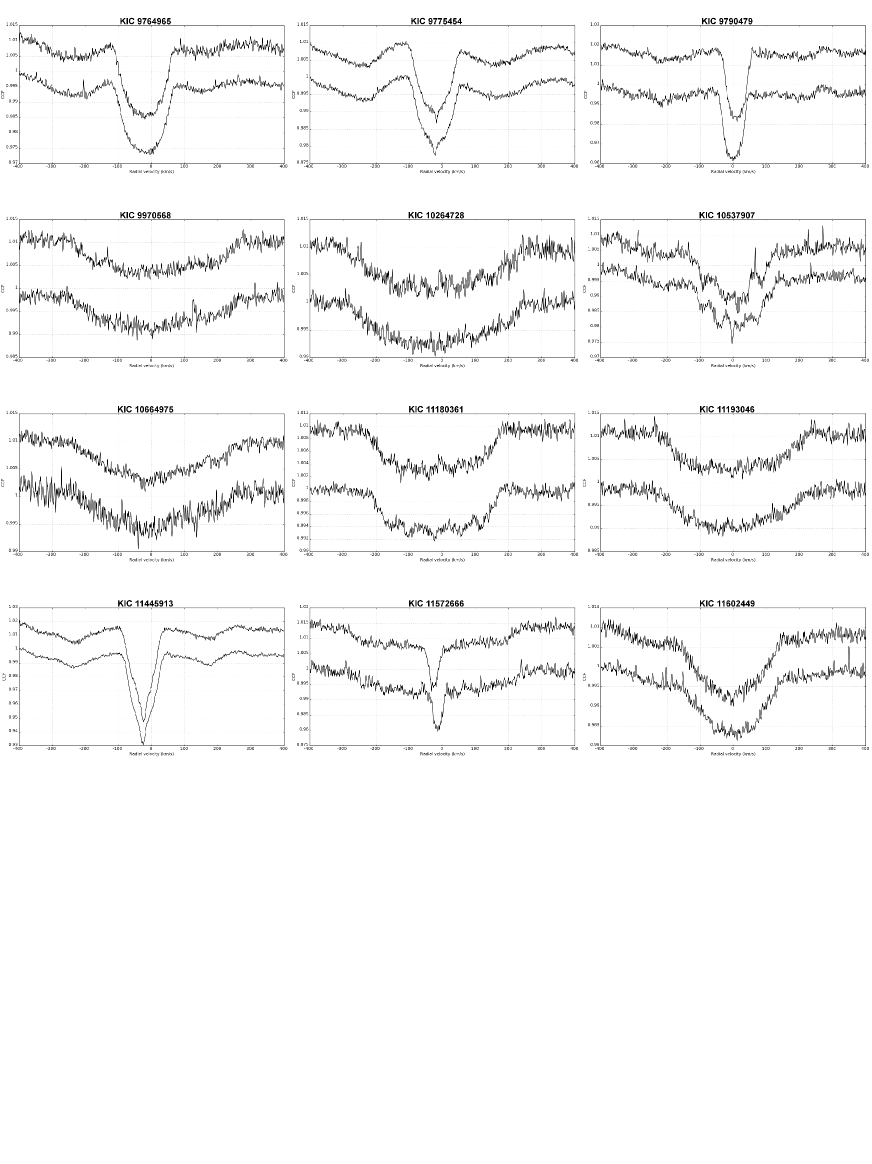
Figure 1: Cross-correlation functions for 48 Kepler objects (cont’ed).

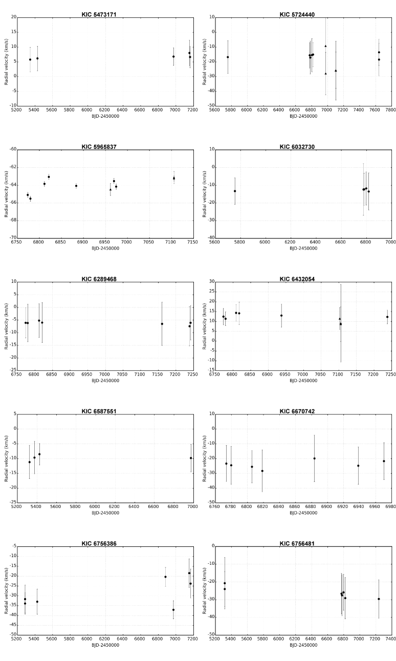
Figure 1: Radial velocity plots for 44 Kepler objects (cont’ed). The same symbols as before are used.

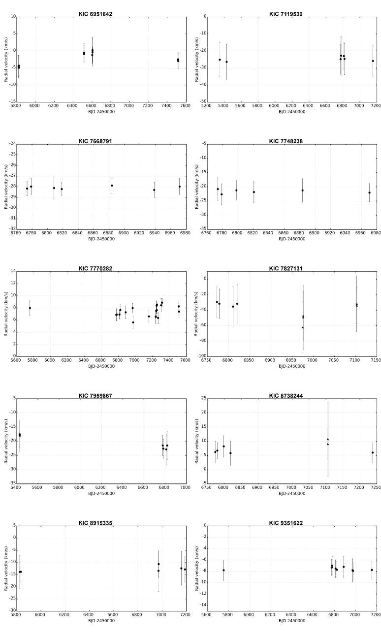
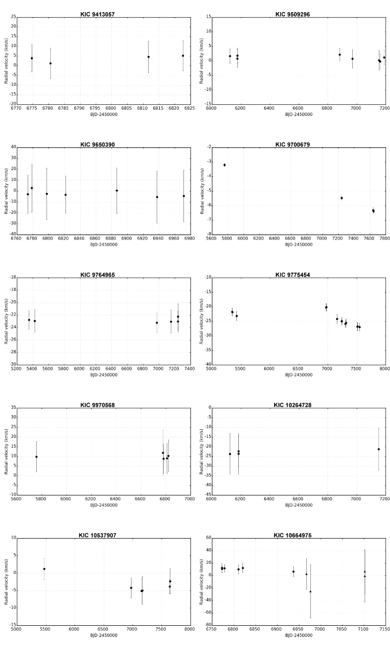
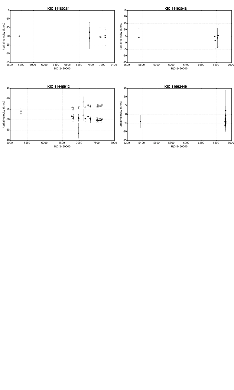
Figure 1: Radial velocity plots for 44 Kepler objects (cont’ed). The same symbols as before are used.

The KIC magnitudes of our targets are brighter than or equal to 10.3 mag. For a target brightness of 9.5 mag, an exposure time of 10 min was usually sufficient to reach a signal-to-noise ratio (S/N) of at least 50 per bin (at $\lambda=650$ nm). The exposure times ranged between 5 and 30 min mostly, leading to a S/N of about 200 in the CCF (with over 100 useful lines in the spectrum). We expected to achieve a precision of 1 km s^-1 in the measurement of the radial velocities in most cases. We acquired a minimum of four high-resolution spectra for all our targets. Sampling was done irregularly over a total time base of four years. We planned at observing each target during two successive nights in the first week, once after at least a full week, and once more after a time lapse of at least one month. This intended scheme could, however, not always be maintained due to practical circumstances. On average, we dispose of 5-10 Hermes spectra per target. Our spectra cover time scales of a few days, weeks and months up to a few years per target. The objective is to be able to (spectroscopically) detect binarity for orbital periods ranging from a day up to a few months. The actual temporal distribution of most spectra is illustrated in Fig. 1.

An additional goal is to determine improved atmospheric stellar parameters and $v\,\mathrm{sin}\,i$ for our targets, in particular for the single-lined cases, in order to pinpoint their position in the H-R diagram. The combination of (at least) four spectra per target allows us to reach a reasonable precision on the effective temperature ($T_{\mathrm{eff}}$) and the surface gravity ($\mathrm{log}\,g$).

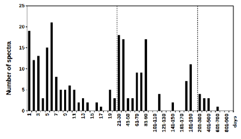
Figure 1: Distribution of time intervals between successive Hermes spectra for the sample stars showing peaks of 1 and 6 days as well as $\sim$1 and $\sim$3 months. Note the rapidly increasing bin size along the X-axis.

3 Data reduction and processing

The spectra were reduced with the dedicated reduction pipeline elaborated for Hermes spectra which includes the subtraction of the bias and stray light, order-by-order extraction, correction for the flat-field, and the scaling in wavelength using calibration frames (obtained with Thorium–Argon lamps) followed by cosmic rays removal and order merging (Raskin et al. 2011). The procedure also provides the S/N, which in our case is in the range of 60-70 (at $\lambda=650$ nm) on average. For all the spectra, the normalisation to the local continuum was done by fitting a low-order polynomial through the continuum parts in wavelength bins of about 50 nm long using the IRAF task ’continuum’. The average S/N of the median spectra is of the order of 150-200.

The Ace spectra were reduced using IRAF standard tasks including bias, aperture extraction, dark and flat-field corrections, and wavelength calibration using Thorium–Argon exposures. The normalisation, cosmic rays filtering, order merging (and cross-correlation, see below) was performed by in-house programmes (developed by ÁS). The systematic errors introduced by the data processing and the stability of the wavelength calibration system of the Ace instrument was found to be better than 0.36 km s^-1, based on observations of radial velocity standards (Derekas et al. 2017). All the spectra were systematically corrected for barycentric motion.

4 Data analysis

As a first-look analysis, we computed a series of one-dimensional cross-correlation functions (CCFs) in the wavelength intervals $415-445,445-510,510-570$ nm using different pre-selected masks. The correlation masks have been built from line lists computed with the code synspec (Hubeny & Lanz 1995). In the case of a double- or multiple-lined system, these one-dimensional CCFs may show striking features such as a variable (strong) asymmetric broadening (Fig. 2) or multiple minima (Fig. 3). Occasionally, a composite profile consisting of a narrow profile embedded in a broader one was also detected (e.g. KIC 11572666, Fig. 16). In the complex situations, using various masks, we were able to estimate the number of components in the system as well as to derive preliminary values for the component’s spectral types and projected rotational velocities.

4.1 Radial velocities

4.1.1 Single stars and single-lined systems

In the following step, we searched for the most adequate set of fundamental parameters by fitting synthetic models (templates) to the spectrum on the basis of a ’minimum distance’ method (i.e. by determining the smallest $\chi^{2}$). Thus, we explored the parameter space in terms of spectral type and $v\,\mathrm{sin}\,i$ and confronted each observed spectrum to a variety of synthetic spectra in four distinct spectral bins chosen in the wavelength interval $415-570$ nm. The synthetic spectra, suitably broadened to the estimated projected rotational velocity, were computed using the code Synspec (Hubeny & Lanz 1995) together with the atlas9 atmosphere models for $T_{\mathrm{eff}}$ ¡ 15000 K and $\mathrm{log}\,g$ = 4 (Castelli & Kurucz 2003). Except for Section 4.2.1.1, the same method will be used for all synthetic spectra discussed from hereon. Upon finding the closest match in parameter space, we adopted this best-fit model and computed the radial velocity by Doppler shifting the synthetic spectrum until it matched the observed spectrum. This procedure was repeated for (typically 10) smaller wavelength bins, and the mean and scatter of the radial velocity measurement (RV) were derived from the values for the different bins, after the outliers were omitted.

4.1.2 Double- or multiple-lined systems

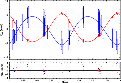
Figure 4: Radial velocities for the mass centre of the inner binary (AB) and for component C of KIC 6381306, plotted over the outer orbital solution with a period of 212 days. The residuals are shown in the bottom part.

In the case of non-single or composite objects, we applied an in-house programme (developed by YF) which uses the algorithm of todcor (Mazeh & Zucker 1994). This code also makes use of Synspec (Hubeny & Lanz 1995) as well as the atlas9 models (Castelli & Kurucz 2003) with the estimated input parameters and $\mathrm{log}\,g$ = 4 to build a suitably broadened synthetic spectrum for each component, and computes the two-dimensional cross correlation and the corresponding radial velocities. It allows us to extract the velocities even when the components are not fully resolved (i.e. the case of blended profiles). We tested different values of spectral type and $v\,\mathrm{sin}\,i$ and adopted the best-fitting parameters based on the same criterion of ’minimum distance’ between the observed and the synthetic composite spectrum. Since the ratio of the light contributions is another free parameter obtained during the fitting, we also derived its most probable value. For illustrations of a triple- and a double-lined system, we refer to Figs. 4 and 5, respectively. Finally, we computed two-dimensional CCFs using this best-fit model for a large number of wavelength bins (usually 10 bins of 6-20 nm long) and derived the mean and scatter of the radial velocities (RVs) from the individual values, after the outliers were omitted.

In the case of a triple-lined system, we repeated this procedure in a two-step sequence: first, with components A and B to search for the best-fitting two-component model and the light ratio $l_{A,B}$ = $l_{B}/l_{A}$, and secondly, adding another component (C) to search for the best-fitting three-component model as well as the additional light ratio $l_{AB,C}$ = $l_{C}/l_{A+B}$.

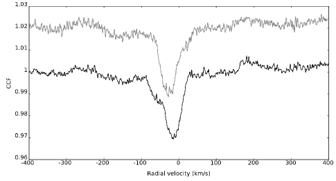
Figure 2: Cross-correlation functions in the case of an unresolved double-lined spectroscopic binary system showing obvious asymmetric profiles as well as velocity shifts e. g. KIC 7756853.

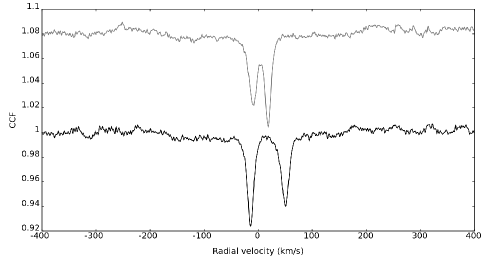
Figure 3: Cross-correlation functions in the case of a well-resolved double-lined spectroscopic binary showing two distinct minima and velocity shifts in its profile e. g. KIC 5219533.

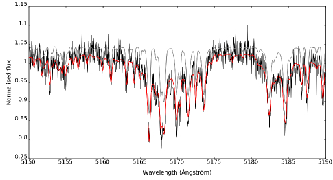
Figure 4: Case of a triple system: part of the spectrum (in black) and composite model (in red) for KIC 4480321 using the synthetic spectra for three components, respectively of type (F0, $v\,\mathrm{sin}\,i$ =10), (F0, $v\,\mathrm{sin}\,i$ =10) and (A5, $v\,\mathrm{sin}\,i$ =160). The thin line (in grey) represents the scaled contribution of the two (F0, $v\,\mathrm{sin}\,i$ =10) components.

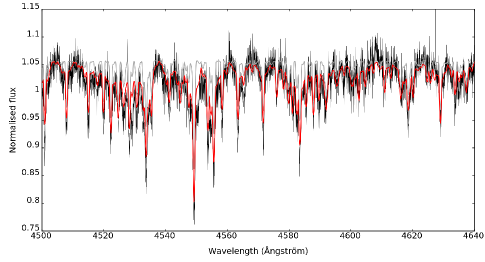
Figure 5: Case of a binary system: part of the spectrum (in black) and composite model (in red) for KIC 8975515 using the synthetic spectra (A7, $v\,\mathrm{sin}\,i$ =170) and (A7, $v\,\mathrm{sin}\,i$ =30). The thin line (in grey) represents the scaled contribution of the (A7, $v\,\mathrm{sin}\,i$ =30) component.

4.2 Atmospheric properties

An additional purpose of the newly acquired spectra is the determination of atmospheric stellar properties. For a reliable characterization and unambiguous location in the Hertzsprung-Russell diagram, the effective temperature and the surface gravity of the selected targets should be known as reliably and accurately as possible. This requires a comparison between observed and synthetic spectra. For single stars and single-lined systems, we fitted several regions of the normalised median spectrum. For non-single objects, we fitted several regions of the normalised individual spectra.

4.2.1 Single stars and single-lined systems

From each spectrum, three regions of width of 45-70 nm centered on the H$\alpha$, H$\beta$, and H$\gamma$ lines, were extracted. Continuum normalisation was performed in two steps: first, by dividing each region of interest by the best-fitting model as defined in Sect. 4.1.1 and secondly, by dividing by a polynomial representation of the local continuum. This low-degree polynomial was computed independently also using sigma clipping. We next combined all the normalised spectra of each region into a normalised single median spectrum of higher quality. These median spectra were subsequently confronted to synthetic spectra using grids computed in slightly different ways.

4.2.1.1 Multi-region fits

Firstly, we performed fits of the three regions of interest containing the lines H$\alpha$, H$\beta$, and H$\gamma$, respectively. An extended grid of high-resolution synthetic spectra computed with plane-parallel model atmospheres was retrieved from the Pollux database (Palacios et al. 2010). We selected the models with a microturbulence of 2 km s^-1 (a typical value for A/F-type MS stars, Gebran et al. (2014)) and a solar metallicity, for which $T_{\mathrm{eff}}$ ranged from 7000 to 9000 K (with a step of 200 K) and $\mathrm{log}\,g$ ranged from 3.5 to 4.9 dex (with a step of 0.2 dex). Only $T_{\mathrm{eff}}$ and $\mathrm{log}\,g$ were varied since the extracted regions include the Balmer lines to a large extent even though they may contain a few shallow metal lines. With this method, the synthetic spectra were selected at the nearest node of the atmospheric values. In general, we adopted the previous estimate for the parameter $v\,\mathrm{sin}\,i$ since it was found to be precisely determined (cf. Sect. 4.1.1). This procedure provided an averaged value of $T_{\mathrm{eff}}$ and a range of probable values for $\mathrm{log}\,g$ which are listed in Table LABEL:tab:param1 (cols. 11-12).

4.2.1.2 Single-region fit

As an independent, final step, we simultaneously (re)derived the three parameters $T_{\mathrm{eff}}$, $\mathrm{log}\,g$ and $v\,\mathrm{sin}\,i$ by fitting the range [415 - 450] nm (including H$\gamma$ cf. Fig. 6) using the code Girfit (Frémat et al. 2006). With this method, the model spectra (cf. description above) are interpolated in a grid of ($T_{\mathrm{eff}}$, $\mathrm{log}\,g$)-values instead of being selected at the nearest node of the atmospheric values. These model spectra were next convolved with the rotational profile as well as a Gaussian instrument profile to account for the spectrograph’s resolution.

The results of this spectrum synthesis method are displayed in Table LABEL:tab:param1 (cols. 13-15). At this point, the probable errors are assumed to be of the order of the grid steps (i.e. $\epsilon_{T_{\mathrm{eff}}}=250$ K for $T_{\mathrm{eff}}$ and $\epsilon_{\mathrm{log}\,g}=0.5$ dex for $\mathrm{log}\,g$), since the procedure uses interpolation. In Sect. 6, we will be able to confirm that such assumptions are also realistic. An example of the adjustment using Girfit for a single object is presented in Fig. 6. Note also the excellent agreement between both determinations (cols. 11-15 in Table LABEL:tab:param1). A direct comparison between the results of both methods furthermore provides a reliable way to estimate the uncertainties involved.

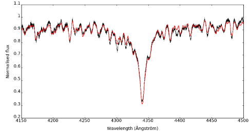
Figure 6: Part of the observed spectrum (in black) for KIC 6432054 and model (in red) using the best-fitting set of atmospheric stellar properties $T_{\mathrm{eff}}$ = 7542 K, $\mathrm{log}\,g$ = 4.44 and $v\,\mathrm{sin}\,i$ = 184 km s^-1 derived with Girfit.

4.2.2 Double- or multiple-lined systems

The programme Girfit was next modified in order to extend the same analysis to spectra with n components (in practice, the spectra of double- and triple-lined systems). The modified programme interpolates the component spectra in the usual grid, and combines them into a composite spectrum to find the solution which minimizes the residuals. The minimisation is performed using the Simplex algorithm. In this extended form of Girfit (developed by YF), the radial velocities and the light ratios can either be kept fixed or be considered as additional free parameters (our choice). The radial velocities served as a consistency check of the solutions, while the light ratios were considered as added value. For each system, we fitted all the individual normalised spectra using various sets of atmospheric input parameters and up to three spectral regions in order to verify the reliability of our results.

5 Classification

Based on the shape of the one-dimensional CCFs and the evolution of the radial velocity measurements with time, we classified each target according to the following categories: S (for stable), VAR (for currently unexplained, possible long-term RV variations), SB (for a spectroscopic binary or triple system), P (for a pulsating star with line-profile variability and/or rotating with the presence of structures on the surface such as chemical spots or temperature gradients) and CMP (i.e. composite, for stars with a narrow, shallow and almost central absorption feature in their – usually – broad profiles). The P-class may contain A/F-type pulsators of the $\delta$ Scuti type where chemical peculiarities appear on the stellar surface due to the presence of a (weak) magnetic field (e.g. KIC 5988140 = HD 188774, Neiner & Lampens 2015) or where stellar rotation is so fast that it deforms the stellar surface and perturbs the homogeneity of the surface intensity distribution (e.g. Böhm et al. 2015). Our determination of $v\,\mathrm{sin}\,i$ alone does not suffice to distinguish between both scenarios. We provide a class for each target of the sample based on the currently available spectroscopic information in Table LABEL:tab:param1 (col. 9). To justify the adopted classification, we provide illustrations for all objects, except for the ones presented in the text, in the form of one-dimensional CCFs (computed with a mask of type F0 in the wavelength range 510-570 nm for all but for KIC 9775454 where we used a K0-mask) as well as radial velocity plots in Appendices A and B, respectively. We present the list of all radial velocity measurements in Tables 1 and 2.

Hereafter, we shortly comment on the classification of various particular targets, including the double- and triple-lined systems. For a detailed description of the orbital solutions, however, we refer to Sect. 7. Further results concerning the classification of the selected targets will come from our analysis of the photometric data of the Kepler mission and their periodograms (cf. Sect. 8).

6 Characterization of stellar atmospheres

Table LABEL:tab:param1 summarises the physical information derived from the study of the CCFs and the spectral analyses. This includes the atmospheric stellar properties (cf. sect. 4.2), as well as the classification of the target into one of the subsequent categories: S (stable), VAR (RV variable), SB(1/2/3) (resp. single-, double-, or triple-lined spectroscopic system), P (pulsating or possibly rotating) or CMP (composite spectrum). We list the following information: the identifier (col. 1), period (col. 2), spectral type (col. 3), $T_{\mathrm{eff}}$ (col. 4), $\mathrm{log}\,g$ (col. 5), and magnitude (col. 6) all from the Kepler Input Catalogue (KIC) except for the spectral type which comes from Uytterhoeven et al. (2011,   Table 1 and references therein), the number of Hermes and Ace spectra collected (col. 7), a comment (col. 8), the classification (col. 9), and the model parameters adopted for reconstructing the (in casu composite) spectrum (col. 10), the mean $T_{\mathrm{eff}}$ (col. 11), the mean $\mathrm{log}\,g$ (col. 12) based on three regions of interest ([620 - 686] nm including H$\alpha$, [450 - 520] nm including H$\beta$, [415 - 460] nm including H$\gamma$), allowing to check for consistency, and, lastly, the $T_{\mathrm{eff}}$ (col. 13), $\mathrm{log}\,g$ (col. 14), and $v\,\mathrm{sin}\,i$ (col. 15) as derived with Girfit in the wavelength range [415 - 450] nm.

We have 28 targets in common with other studies. This allowed us to perform a useful comparison. Table b summarises the atmospheric stellar properties derived from this work, together with some recently published values. The referred studies are mentioned in the footnotes (col. 16 from Table b). In Figures 7, 8, and 9 we illustrate the overall agreement between the various determinations. In particular, the agreement is excellent in $T_{\mathrm{eff}}$ and $v\,\mathrm{sin}\,i$. The scatter in $T_{\mathrm{eff}}$ matches well the estimated uncertainty of $\pm$ 250 K (Fig. 7). While there is clearly no systematic trend in $v\,\mathrm{sin}\,i$, there seems to exist a small systematic offset in $T_{\mathrm{eff}}$ in the temperature range [7300-7700] K. Our temperature values appear to be slightly overestimated in this range with respect to the published values (or vice versa). This effect reminds us of the (known) fact that the KIC-values for $T_{\mathrm{eff}}$ less than 7700 K are believed to be systematically underestimated. The scatter in $v\,\mathrm{sin}\,i$ reflects well the estimated uncertainty of $\pm$ 5-10 km s^-1  but this depends a little on the absolute value (Fig. 9). Two extremely fast rotating stars deviate from the 1:1 ratio line. The determination of $\mathrm{log}\,g$, on the other hand, shows a huge spread which reflects its large uncertainty. It appears from Fig. 8 that some of the literature values were arbritarily set (or limited) to 4. This is often the case for targets cooler than 7700 K (open symbols). We also should mention that a comparison between previously published values (when possible) shows a similar degree of inconsistency, meaning that the errors are larger than thought. In five cases (e.g. KIC 3429637 (Am), KIC 5965837, KIC 9509296, KIC 9764965 (Am), and KIC 10537907), our determination of $\mathrm{log}\,g$ is very different from that of Catanzaro et al. (2011) or Niemczura et al. (2015). Two such cases (KIC 3429637 and KIC 5965837) are treated in detail in the discussion of the 22 individual targets hereafter. The remaining lack of agreement might also be due to the choice of the spectral intervals which may not be very sensitive to $\mathrm{log}\,g$ for stars in the temperature range below 8000 K. Still, we conclude that there is no sign of any systematic trend in this plot and that other data points tend to follow the 1:1 ratio line, illustrating the existence of a rough agreement.

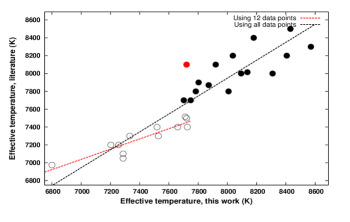
Figure 7: Comparing the various determinations of $T_{\mathrm{eff}}$. A linear fit using the literature values less than 7600 K (open symbols) shows an obvious discrepancy in the slope, illustrating the fact that our values for $T_{\mathrm{eff}}$ less than 7700 K are systematically a little larger than the literature values. The outlier (red symbol) is KIC 7119530 for which two very different literature values were found.

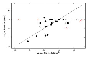
Figure 8: Comparing the various determinations of $\mathrm{log}\,g$. Same symbols as in Fig. 7. The largest differences (red symbols) are found for KIC 3429637 (A9m), 5965837 (F2p) , 9509296, 9764965 (Am), and 10537907.

Figure 9: Comparing the various determinations of $v\,\mathrm{sin}\,i$. Same symbols as in Fig. 7. The largest differences (red symbols) are found for KIC 7119530 and 7827131.

Searching for common targets also based on lower resolution spectra, we identified 22 targets (26 measurements) in common with the Lamost project (De Cat et al. 2015). In Table c, we compare the atmospheric stellar properties derived from this work to those derived by the Lamost teams using the procedure Rotfit (Frasca et al. 2003, 2016). In four cases, different values were derived from the Lamost spectra (with a resolution of R $\sim$ 1800). Large differences, in $\mathrm{log}\,g$ mostly, occur for the two fast rotators KIC 3453494 and KIC 9650390, as well as in the case of KIC 7748238 (because of our large value of $\mathrm{log}\,g$ ). In two cases (KIC 7668791 and KIC 9650390), our value of $T_{\mathrm{eff}}$ differs from that of the Lamost team, though our determinations of both $T_{\mathrm{eff}}$ and $\mathrm{log}\,g$ agree very well with the KIC values. This comparison illustrates the fact that the largest differences occur more often in the fast rotating A/F-type stars (for which the estimated errors are also large).

6.1 KIC 3429637 = HD 178875

HD 178875 is not a candidate A/F-type hybrid star from Uytterhoeven et al. (2011). This object was classified as a normal $\delta$ Scuti star while being suspected of binarity (Catanzaro et al. 2011). For this reason, we included it in our programme. The RV data show variability with an amplitude smaller than $\sim$ 5 km s^-1 on a time scale of several months, but no day-to-day variations (cf. Appendix B). We found no direct trace of spectroscopic duplicity. Since we also detected line profile variations in the CCFs, we classified it as a pulsator accompanied by a long-term RV variability (“P+VAR”). We obtained the following stellar properties: $T_{\mathrm{eff}}$ = 7266 K, $\mathrm{log}\,g$ = 2.66, and $v\,\mathrm{sin}\,i$ = 49 km s^-1. While there is a good agreement in $T_{\mathrm{eff}}$ and $v\,\mathrm{sin}\,i$ with Catanzaro et al. (2011), we however do not confirm their value of $\mathrm{log}\,g$ = 4. In Fig. 8, we notice a corresponding large discrepancy. We confirm its status of evolved Am star (cf. Murphy et al. 2012). Since this star is known to have a peculiar spectral type (kF2hA9mF3), its non-standard surface composition may interfere with the gravity determination.

6.2 KIC 3453494

The CCF profiles of this fast rotating star (estimated $v\,\mathrm{sin}\,i$ of 220 km s^-1) are extremely broad and noisy which makes it difficult to detect any kind of variability. Nothwithstanding the noise and given the limited accuracy, we conclude that the radial velocity and the profiles are stable (“S”). We encountered several other cases of extreme stellar rotation, namely KIC 6756481, 7119530, 7827131,  9650390 and 11602449, as well as KIC 4989900 and 6670742 (the latter two classified as “S/P?”, with some ambiguity in their classification) (cf. Sect. 10).

6.3 KIC 4480321

This object is a new spectroscopic triple system (SB3). The spectrum shows the presence of a twin-like inner binary orbiting a slightly more luminous and fast rotating third component (cf. Fig. 4 and the CCF profiles in Appendix A). We have excellent RV coverage for the close binary system and estimate the uncertainty of the component RV measurements to be significantly smaller than 1 km s^-1. From two campaigns of 11 nights each, we derived an initial value near 9 days for the orbital period of the close binary. An orbital solution for the inner binary is presented in Sect. 7. A tentative orbital solution for the outer system is also provided, though the period is probably longer than the available time span.

Using a composite model consisting of three synthetic spectra (A5, $v\,\mathrm{sin}\,i$ = 160), (F0, $v\,\mathrm{sin}\,i$ = 10) and (F0, $v\,\mathrm{sin}\,i$ = 10), we were able to reconstruct parts of the observed spectra very well (see Fig. 4). We next applied the extended 3-D version of Girfit in three different regions of the normalised spectra using a composite model to find the solution which minimizes the residuals between the model and the observations. We fixed the $\mathrm{log}\,g$ values to 4 (for MS phase) and the projected rotational velocities to our previous estimations (of resp. 160 km s^-1, 10 km s^-1 and 10 km s^-1), and varied the initial values for the effective temperatures and the two luminosity ratio’s (the only free parameters left). We found the component effective temperatures of $T_{\mathrm{eff}}$₁ = 7900 $\pm$ 100 K with both $T_{\mathrm{eff}}$₂ and $T_{\mathrm{eff}}$₃ in the range between 6300 and 6900 K (probably of similar temperature) in accordance with some of the observed spectra. However, no unique solution was found which would fit all our spectra in any of the inspected wavelength regions [415 - 450], [500 - 520] or [630 - 680] nm. The component properties are thus not well-known. We conclude that high-S/N spectra would be crucial for a more precise component characterization of this triple system.

6.4 KIC 5219533

This target forms a visual double system with HD 189178 (5.5 mag, component A) at an angular separation of 65″. It is a well-resolved, double-lined spectroscopic system (cf. Fig. 3), with a primary component of type Am (A2-A8, Renson & Manfroid 2009). We furthermore deduce the presence of a more rapidly rotating component of a slightly cooler spectral type based on two arguments: (a) from the unusual aspect of the (component and systemic) radial velocities (cf. Appendix B), and (b) from a comparison of the observed spectra with models. For example, we found that a two-component synthetic spectrum is unable to reproduce the broad features found in various parts of the spectrum (cf. Fig. 10). We therefore conclude that this object is a new triple-lined spectroscopic system (SB3). An orbital solution for the inner binary is presented in Sect. 7.

In order to compute reliable values for the component’s atmospheric parameters and because the third component is very diluted, we applied the 2-D version of Girfit onto different regions of the normalised observed spectra in search of the 2-component model which best minimizes the residuals. Due to the complexity of this spectrum, we fixed the $\mathrm{log}\,g$ values to 4 and kept the projected rotational velocities constant by adopting our previous estimations of $v\,\mathrm{sin}\,i$ (i. e. 10 km s^-1 for both components). The component effective temperatures and the luminosity ratio were the only free parameters. Allowing for more free parameters did not allow us to find any reliable solution. We chose various initial values and spectral regions, which gave us estimates for the uncertainties on the free parameters. Though both components are usually well-resolved, we were unable to find a unique solution for all our spectra. The most promising results were obtained in the interval [500 - 520] nm, where a consistent solution was found for most spectra (7 out of 12). In this case, the mean effective temperatures of $T_{\mathrm{eff}}$₁ = 8300 $\pm$ 100 K and $T_{\mathrm{eff}}$₂ = 8200 $\pm$ 100 K coupled to a light ratio l₁ equal to 0.53 $\pm$ 0.02 were obtained. This indicates that the pair might consist of nearly identical “twin” stars of spectral type A5. In the ranges [415 - 450] nm and [640 - 670] nm, however, a more pronounced temperature difference between the components was derived but the solutions from the individual spectra showed less consistency. Since our models assume a standard solar composition, possible explanations for this behaviour might be the non-standard metallicity of the component(s) or the influence of the diluted third companion. A few spectra of high(er) S/N will be needed to improve the characterization of this new triple system.

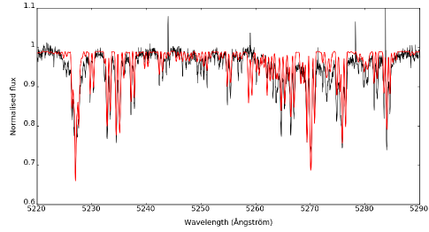
Figure 10: Observed spectrum of KIC 5219533 (in black) vs. model spectra consisting of two narrow-lined components (in red). An extra broad-lined component of a similar spectral type could explain the additional wings and parts with missing continuum.

6.5 KIC 5724440

The CCF presents an extremely broad profile together with some additional features which seem to be variable. The broad profile appears to be stable in RV. We classified this target as “P?”. The fast rotation could be the reason why previous determinations of $T_{\mathrm{eff}}$ showed a large scatter (Catanzaro et al. 2011), but our value matches perfectly both the spectroscopic determination by Niemczura et al. (2015) and the photometric one by Masana et al. (2006). This object closely resembles KIC 6432054 which was also classified as a pulsator.

6.6 KIC 5965837

The CCF presents a narrow profile which is reflected by the extremely low $v\,\mathrm{sin}\,i$. The changes in the profile core are obviously due the presence of non-radial pulsations (classified as “P”, cf. Appendix A). The radial velocities show a distinct variable pattern with a very low amplitude, a possible indication of radial pulsation. It is the coolest candidate hybrid star in our sample. We derived the following stellar properties: $T_{\mathrm{eff}}$ = 6800 K, $\mathrm{log}\,g$ = 3.3 and $v\,\mathrm{sin}\,i$ = 15 km s^-1. While there is an excellent agreement in $T_{\mathrm{eff}}$ and $v\,\mathrm{sin}\,i$, we cannot confirm the value of $\mathrm{log}\,g$ = 4 (Catanzaro et al. 2011). Instead, we derived $\mathrm{log}\,g$ = 3.3 based on the Mg ii triplet using the spectral range [510-520] nm. Furthermore, we discovered that its chemical composition is non-standard, and heavily enhanced in metals. In fact, this star’s spectrum almost perfectly matches that of 20 CVn, a well-known $\rho$ Puppis star (Fig. 11). In conclusion, KIC 5965837 is a newly discovered $\rho$ Puppis star, i.e. an evolved and cool giant star with a metal-rich surface composition also showing pulsations. This is an interesting Kepler star for a detailed study in view of the co-existence of pulsation and metallicism (Kurtz et al. 1995).

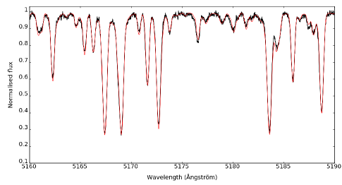
Figure 11: Part of the observed spectrum for KIC 5965837 (in black) and corresponding part of the elodie spectrum of 20 CVn artificially broadened to the same rotation velocity ($v\,\mathrm{sin}\,i$ = 15 km s^-1) (in red).

6.7 KIC 6381306

This object is another new spectroscopic triple system (SB3). It consists of a “twin”-like binary and a slightly more luminous, more rapidly rotating primary component. For the inner binary system, we estimated an orbital period of $\sim$ 4 days. For the outer system, a periodicity of between about 100 and 200 days is expected. Both orbital solutions are presented in Sect. 7.

We applied the extended 3-D version of Girfit in different regions of each spectrum to find the solution which best minimizes the residuals. The model spectrum is a composite of three components. We fixed the $\mathrm{log}\,g$ values to 4 and the projected rotational velocities were set close to our previous estimations (resp. 90-100 km s^-1, 5-10 km s^-1 and 5-10 km s^-1). The component effective temperatures and two luminosity ratio’s were the only free parameters left. We chose various initial values for these input parameters. Very similar results were found across both intervals [415 - 450] and [500 - 520] nm, though a consistent solution for only half out of 13 spectra was obtained at best. From these computations, we obtained the mean effective temperatures of $T_{\mathrm{eff}}$₁ = 9000 $\pm$ 100 K, $T_{\mathrm{eff}}$₂ = 7400 $\pm$ 100 K, and $T_{\mathrm{eff}}$₃ = 7200 $\pm$ 50 K coupled to light factors of 0.79, 0.11 and 0.10 (for l₁, l₂ and l₃, respectively). It is moreover evident that such a complex model requires spectra of high(er) S/N ratio for a better characterization of this system.

6.8 KIC 6756386 and KIC 6951642

Both objects have been classified as“P+VAR”. Their CCF profiles show clear line-profile variations which are due to the presence of stellar pulsations (cf. Appendix A). In addition, the temporal evolution of both RV data sets indicates a long-term variability with a low amplitude, whose origin cannot yet be determined (cf. Appendix B).

6.9 KIC 6756481 and KIC 7119530

The CCFs present an extremely broad profile but with an additional sharp-peaked feature (cf. Appendix A). Unlike the case of the very fast rotator KIC 5724440, we verified that the narrow central feature of KIC 6756481 remains constant on the velocity scale, suggesting the possible presence of a circumstellar shell. In such a case, the broad lines would correspond to the stellar photosphere and the narrow central ones to a circumstellar shell (e.g. Mantegazza & Poretti 1996). In the case of KIC 7119530, this feature is near central and appears to be stronger in the red part of the spectrum. The radial velocities of the broad absorption profiles are constant (cf. Appendix B). In Fig. 12, we compare the H$\alpha$ profile of KIC 6756481 with that of KIC 6670742 of the same $T_{\mathrm{eff}}$ and $v\,\mathrm{sin}\,i$ to look for a sharp absorption core (e.g. Henry & Fekel 2003). We see that both profiles are almost identical except in the small core region where KIC 6756481’s profile is sharper and a bit deeper. In the case of KIC 7119530, we found a perfect match with the H$\alpha$ profile of KIC 4989900 (of the same $T_{\mathrm{eff}}$ and $v\,\mathrm{sin}\,i$ ). We classified both stars as “CMP” (which stands for composite spectrum). Their atmospheric parameters are close though not exactly identical, see e.g. the large projected rotational velocity of KIC 6756481. Due to its fast rotation, the uncertainties on the radial velocities are larger than usual, which makes it very difficult to detect any trace of variability. Similar cases among the late A/early F-type stars known in the literature are seven objects which were reported as possible shell stars by Fekel et al. (2003). An alternative explanation is that these objects consist of (at least) two components of similar type and without any detectable RV variation on the short term scale. Such physical cause was eventually confirmed (Henry & Fekel 2003), as well as more recently by Fekel (2015a) for the triple system HD 207561.

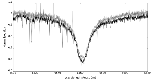
Figure 12: Comparison of two H$\alpha$-profiles: KIC 6756481 (plotted in black) versus KIC 6670742 (in grey).

6.10 KIC 7756853

The CCF shows a highly variable, sometimes asymmetric, profile due to the presence of a companion (cf. Fig. 2). The variations of the RVs with time confirm the detection as a new double-lined spectroscopic binary (SB2). Both components present a $v\,\mathrm{sin}\,i$ difference of about 20 km s^-1 (Table LABEL:tab:param1). We applied the 2-D version of Girfit in different regions of each spectrum to find the solution which best minimizes the residuals. We explored the parameter space by varying the number as well as the initial values of the input parameters. To restrict the number of free parameters, we used our previous estimations of $\mathrm{log}\,g$ and projected rotational velocity. The latter appeared to be reliable and very consistent, in such a way that we kept their values fixed in most fits. The $\mathrm{log}\,g$ values of the models were fixed to the value 4 (MS phase). This also provided estimates of the uncertainties on the adopted input parameters.

While a good match was found with a model consisting of an A1-type primary with $v\,\mathrm{sin}\,i$₁ = 50 km s^-1 and an A5-type secondary with $v\,\mathrm{sin}\,i$₂ = 30 km s^-1 during the initial analysis, the actual process converged towards a pair of solutions signalling the existence of (at least) two minima. Imposing $\mathrm{log}\,g$ = 4 and $v\,\mathrm{sin}\,i$, a first stable solution was found in the region [415 - 450] nm with $T_{\mathrm{eff}}$₁ = 9600 $\pm$ 100 K and $T_{\mathrm{eff}}$₂ = 8260 $\pm$ 60 K and a light factor l₁ equal to 0.61 $\pm$ 0.03, but another stable solution was also found with a light factor l₁ equal to 0.54 after reversing the assignment of $v\,\mathrm{sin}\,i$ to the components. This smaller light factor indicates compensation for the fact that the $v\,\mathrm{sin}\,i$ value corresponding to the component with the lower $T_{\mathrm{eff}}$ is larger.

In the region [500 - 520] nm, where the residuals were smallest, a first stable solution with a larger temperature differences was found with $T_{\mathrm{eff}}$₁ = 9880 $\pm$ 100 K and $T_{\mathrm{eff}}$₂ = 7480 $\pm$ 170 K and a light factor l₁ equal to 0.73 $\pm$ 0.04 (model A). However, exchanging the values of $v\,\mathrm{sin}\,i$, we found a second stable solution with $T_{\mathrm{eff}}$₁ = 9980 $\pm$ 120 K and $T_{\mathrm{eff}}$₂ = 7300 $\pm$ 140 K and a light factor l₁ equal to 0.66 $\pm$ 0.04 fitting all our spectra equally well (model B). Including $v\,\mathrm{sin}\,i$ as extra free parameters, similar values of $T_{\mathrm{eff}}$ were retrieved. Model B thus consists of an A1-type primary with $v\,\mathrm{sin}\,i$₁ = 27 $\pm$ 5 km s^-1 and an A5/F0-type secondary with $v\,\mathrm{sin}\,i$₂ = 57 $\pm$ 5 km s^-1. The distinction between the different solutions is hard to make as the computed composite spectra look very similar except for a few blended absorption lines. We compared both possible models with a single observed spectrum in the range [415 - 450] nm and observed that the noise level in the spectrum does not allow to distinguish between them. To allow for better discrimination, we simulated the composite cross-correlation function for each model using a mask of spectral type A4 (Fig. 13). This comparison shows that model B represents the observed composite CCF more adequately than model A. This is also confirmed by the residual values. In addition, we compared two spectra with the solutions of model B in the spectral range [386 - 404] nm. In this range, the solution with the higher temperature ($T_{\mathrm{eff}}$₂ = 8400 K) reproduces the Ca ii line ($\lambda$ = 393 nm) very well. This binary is clearly a difficult study case due to the large blends between the components. We tentatively adopted the solution named ’model B’ found in the region [500 - 520] nm.

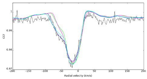
Figure 13: Observed versus modelled CCF in the case of KIC 7756853. The spectral range used is [415 - 450] nm. Model A is shown in green/lilac while model B is shown in (light/dark) blue.

6.11 KIC 7770282

The CCF profiles show clear asymmetric variations which were first attributed to the presence of a companion. Upon closer inspection, however, we found that the CCF shape is maximally distorted in the core and the red wing only, while the blue wing remains apparently unaffected (cf. Fig. 14). The RV data indicate a scatter higher than normal and thus possible variability of amplitude smaller than a few km s^-1, but we attribute this RV scatter to the line profile variations (cf. Appendix B). We believe that the distortions seen in the CCFs are caused by features which are located at the stellar surface. They could be the signature of pulsations (”bumps“) or rotational modulation (”spots“). It should also be remarked that the dominant period found in the Kepler photometry is almost equal to one day. We conclude that this object is (most) probably not a spectroscopic binary, but should rather be considered as “P”. It deserves to be re-examined in the light of several high(er) quality spectra.

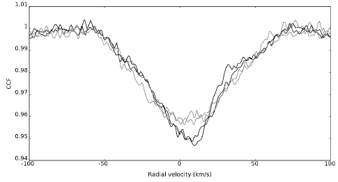
Figure 14: CCF profiles of four different spectra of KIC 7770282. They illustrate the largest observed distortions.

6.12 KIC 8975515

This object is another new double-lined spectroscopic system (SB2) with an orbital period of at least 1000 days. The RV curve presents a clear, well-defined modulation of the slowly rotating component with an amplitude smaller than 10 km s^-1. An orbital solution for this long-period binary system is presented in Sect. 7.

Unlike the case of KIC 5219533, both components have dissimilar projected rotational velocities (cf. Fig 5 and CCF profiles in Appendix A). Therefore, we let the component effective temperatures, the $v\,\mathrm{sin}\,i$’s and the luminosity ratio be free parameters but fixed the $\mathrm{log}\,g$ values to 4. As for KIC 5219533, a wide variety of initial values and spectral regions was explored in the search for a consistent solution. In this case also, we observed that the resulting values depend on the chosen spectral region. In the interval [415 - 450] nm, the mean effective temperatures of $T_{\mathrm{eff}}$₁ = 6800 $\pm$ 20 K and $T_{\mathrm{eff}}$₂ = 8250 $\pm$ 4 K coupled to $v\,\mathrm{sin}\,i$’s of respectively 161 $\pm$ 1 and 32 $\pm$ 1 km s^-1 with a light ratio l₁ equal to 0.49 $\pm$ 0.02 were obtained. In the interval [500 - 520] nm, the mean effective temperatures of $T_{\mathrm{eff}}$₁ = 7440 $\pm$ 20 K and $T_{\mathrm{eff}}$₂ = 7380 $\pm$ 21 K coupled to $v\,\mathrm{sin}\,i$’s of respectively 164 $\pm$ 0.5 and 31 $\pm$ 1 km s^-1 with a light ratio l₁ equal to 0.65 $\pm$ 0.03 were obtained. In the interval [640 - 670] nm, the mean effective temperatures of $T_{\mathrm{eff}}$₁ = 6960 $\pm$ 150 K and $T_{\mathrm{eff}}$₂ = 7850 $\pm$ 150 K coupled to $v\,\mathrm{sin}\,i$ ’s of respectively 154 $\pm$ 2 and 32 $\pm$ 1 km s^-1 with a light ratio l₁ equal to 0.51 $\pm$ 0.04 were obtained. Since the residual sum of squares (RSS) of all our spectra is much smaller in the [500 - 520] nm interval, we decided to adopt the atmospheric parameters derived from this region. This indicates that the pair might consist of two nearly identical stars of type A8. The projected rotational velocities $v\,\mathrm{sin}\,i$₁ and $v\,\mathrm{sin}\,i$₂ are safely determined to be 162 $\pm$ 2 and 32 $\pm$ 1 km s^-1. In the ranges [415 - 450] nm and [640 - 670] nm, however, a more pronounced temperature difference (of $\sim$ 1000 K) between the components was found, as in some other cases. Follow-up as well as high(er) S/N spectra will be required to obtain more accurate component properties of this system.

6.13 KIC 9700679

The few Hermes spectra that were acquired indicate an obvious shift in the radial velocity (cf. Appendix B). This object is another single-lined spectroscopic system (SB1). Since it has a KIC temperature of about 5070 K, it is (much) too cool to be considered as a potential A/F-type hybrid star.

6.14 KIC 9775454

The CCF (computed with a mask of type K0 instead of F0) presents clear distortions in shape, accompanied by the presence of a narrow feature which moves but remains close to the central position. Furthermore, we detected a change of small amplitude in RV (cf. Appendix A). This is most certainly another long-term spectroscopic binary system. We classified this object as “SB1”, though some lines due to the secondary component obviously affect the observed spectrum (the companion is difficult to detect, until we obtain radial velocities for the secondary, we will not use the “SB2” classification). Based on the appearance of the RV curve (cf. Appendix B), we suggest a simple estimate of the order of 1700 days for the period. We plan to continue the RV monitoring of this system and to search for an orbital solution of type SB2. Since the time-delay (TD) analysis supports the existence of a similar periodicity (cf. Sect. 8), we furthermore intend to combine both data types into a joint analysis in the future. This object is one of the coolest objects of the sample.

6.15 KIC 9790479

The CCF presents a probable stable profile accompanied by long-term variations in RV. We classified it as a single-lined spectroscopic binary (SB1). A possible orbital period is of the order of 230 days (see Fig. 22 in Sect. 7). This system needs follow-up observations during the next two years.

6.16 KIC 10537907

The CCF profiles clearly show the signature of pulsations (cf. Appendix A), also accompanied by a small shift in RV on a time scale of $\sim$ 1500 days (cf. Appendix B). We classified it as a probable single-lined spectroscopic binary with pulsations (“P+SB1”). The system also needs additional follow-up observations.

6.17 KIC 10664975

Some CCF profiles of higher quality display features in the form of ”moving bumps“ probably caused by pulsations (cf. Appendix A), while the RV data are stable (cf. Appendix B). We thus classified it as a pulsator (”P“).

6.18 KIC 11180361

The CCF shows an extremely broad and noisy profile which also appears to be stable in RV (cf. Appendix B). This target (KOI-971) is a new Kepler eclipsing binary system (Slawson et al. 2011) with an orbital period of 0.2665 days (instead of the Kepler value of 0.5330 days). It has been classified as stable (“S”) based on our adopted criteria. This means that the secondary component does not visibly affect the observed spectrum.

6.19 KIC 11445913

The CCFs show a superposition of two components (cf. Appendix A). This is a new double-lined spectroscopic system (SB2) consisting of an early F-type star with a K-type companion, both with a low $v\,\mathrm{sin}\,i$ (Fig. 15). The primary component is probably of type Am. The variations in RV indicate a long-term change, mostly due to one older measurement and another measurement apparently in anti-phase with respect to the remainder of the data (cf. Appendix B). The orbital period is not yet known.

A variety of initial values and spectral regions was explored in the search for a consistent match between the observed spectra and the models. We let the component effective temperatures, the $v\,\mathrm{sin}\,i$ ’s and the luminosity ratio be free parameters while fixing the $\mathrm{log}\,g$ values to 4. Here again, the best fits were obtained in the [500 - 520] nm interval. Thus, we decided to adopt the atmospheric parameters derived from this region. The mean effective temperatures of $T_{\mathrm{eff}}$₁ = 7180 $\pm$ 20 K and $T_{\mathrm{eff}}$₂ = 5750 $\pm$ 21 K coupled to $v\,\mathrm{sin}\,i$’s of respectively 55 $\pm$ 1 and 8 $\pm$ 4 km s^-1 with a light ratio l₁ equal to 0.95 $\pm$ 0.01 were obtained. This solution was found to be consistent with all our spectra. In the [630 - 680] nm interval, the temperature difference between the components appeared to be about 500 K larger, though the quality (in terms of RSS) is worse. This system definitely deserves more follow-up observations in the next years.

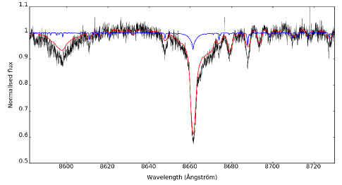
Figure 15: Observed versus modelled spectrum for KIC 11445913 showing the two distinct contributions in red and blue. The plotted range includes the Paschen series as well as the Ca triplet.

6.20 KIC 11572666

KIC 11572666 is another double-lined spectroscopic binary whose lines are strongly blended, with one extremely broad and one narrow component (SB2). It is very similar to the systems analysed by Fekel et al. (2003). We used the extended version of Girfit to derive the component’s spectral characteristics. For each observed spectrum, we chose several models and used different initial values based on our previous estimations of the spectral types and the projected rotational velocities. Here, we also let the projected rotational velocities as well as the $\mathrm{log}\,g$ values be free parameters. For consistency, we repeated the fitting process with both $\mathrm{log}\,g$’s fixed to 4 (MS phase). In this case, a unique model appeared to be compatible with all our spectra. In the spectral range [415 - 450] nm, we found the mean parameters $T_{\mathrm{eff}}$₁ = 7950 $\pm$ 40 K, ($\mathrm{log}\,g$₁ = 3.9 $\pm$ 0.2 or 4 (fixed)), $v\,\mathrm{sin}\,i$₁ = 267 $\pm$ 5 km s^-1 in combination with $T_{\mathrm{eff}}$₂ = 6000 $\pm$ 150 K, $\mathrm{log}\,g$₂ = 4 (fixed) and $v\,\mathrm{sin}\,i$₂ = 22 $\pm$ 3 km s^-1. In the spectral interval [500 - 520] nm, we derived $T_{\mathrm{eff}}$₁ = 7900 $\pm$ 80 K, $v\,\mathrm{sin}\,i$ ₁ = 253 $\pm$ 2 km s^-1 in combination with $T_{\mathrm{eff}}$₂ = 6150 $\pm$ 200 K and $v\,\mathrm{sin}\,i$₂ = 20 $\pm$ 2 km s^-1. Both solutions agree with each other, the model consists of a rapidly rotating F0-type primary with $v\,\mathrm{sin}\,i$₁ = 250 km s^-1 and a F/G-type secondary with $v\,\mathrm{sin}\,i$₂ = 20 km s^-1. We also simulated the composite cross-correlation function using a mask of spectral type A4 (Fig. 16). This plot shows that the adopted model represents the observed composite CCF extremely well. The RVs were previously determined using the model of an A5-type primary with $v\,\mathrm{sin}\,i$₁ = 250 km s^-1 and an F3-type secondary with $v\,\mathrm{sin}\,i$₂ = 20 km s^-1. The RVs of the secondary component are very well-defined, whereas those of the primary component are only poorly determined due to its fast rotation (cf. Fig. 23). This system contains a primary component of type Am and requires further RV monitoring.

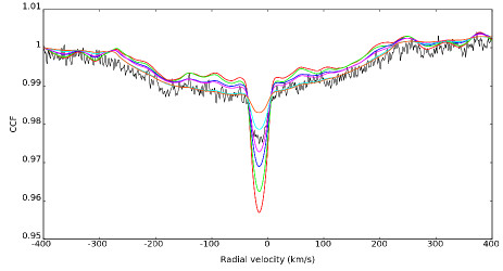
Figure 16: Observed versus modelled CCF in the case of KIC 11572666. The combinations used for the models are F0-G2, F0-F3, A7-G2, A7-F3, A5-G2 and A5-F3. The closest match is found for the model with two early F-type components of very different $v\,\mathrm{sin}\,i$ (shown in light blue). The next best match is for the A7-G2 model (shown in pink).

7 Multiplicity rate and orbital solutions

We repeatedly observed 50 targets as well as KIC 3429637 (previously classified as a $\delta$ Scuti star) with Hermes and Ace, and we found direct evidence for spectroscopic duplicity in ten cases. This concerns the single-lined (SB1) systems KIC 9700679, 9775454 and 9790479, the double-lined (SB2) systems KIC 7756853, 8975515, 11445913 and 11572666 and the triple-lined (SB3) systems KIC 4480321, 5219533 and 6381306. The number of well-detected new spectroscopic systems represents 20% of the total sample. Furthermore, we also identified two extremely fast rotators where a narrow and almost central feature can be noticed superposed onto a very broad stellar profile which we classified as “C(o)MP(osite)” (i.e. KIC 6756481 and 7110530). In both cases, the central feature might be linked to the existence of a shell-like contribution or to an unknown stellar companion (Fekel 2015b).

With respect to the sample of A/F-type candidate hybrid stars, we will not consider KIC 9700679 which is too cool for an A/F-type star in the following discussion. Thus, we detected nine spectroscopic systems among 49 targets. In addition, we should consider the targets with a long-term and low-amplitude variability of their radial velocities classified as “VAR”, as these may turn out to be (mostly single-lined) long-period systems. The number of such detections is three, which gives a total number of 12 (out of 49), corresponding to a spectroscopic multiplicity fraction of 24%. If we add to this the known eclipsing binary KIC 11180361, we derive a global multiplicity fraction of 27%. This number indicates that at least 1/4 of our sample of candidate hybrid stars belongs to a binary or a multiple system of stars.

For four systems (with periods smaller than 100 days), our RV measurements have sufficient phase coverage to allow a reliable determination of the orbital period and a search for an orbital solution. In six more cases (of which three refer to different systems), we propose a preliminary or plausible orbital solution only. In all the remaining cases, the RVs plotted as a function of time are found in Appendix B.

7.1 KIC 4480321

We computed a best-fitting orbital period of 9.2 days using Period04 (Lenz & Breger 2014). This result was subsequently refined using an updated version of the Fortran code vcurve_SB for double-lined systems (priv. commun. IvS, Leuven). The presence of the third component influences the systemic velocity of the inner binary, thus we allowed for systematic offsets of its value with time. Both component RV curves are illustrated in Fig. 17. The residuals are small and homogeneously distributed around null. The final orbital parameters are listed in the upper panel of Table 4.

Concerning the wide system (AB-C), we found that orbital periods of the order of the time span (e.g. a period of 1500 days) or longer provided convincing solutions. Based on the currently available RVs, the best possible outer orbital solution (in terms of rms) has a period of about 2280 days. The RV curves of the centre of mass of the close pair AB, together with that of component C, illustrating the solution are displayed in Fig. 2 (Appendix B). The parameters of this tentative orbital solution are listed in the bottom panel of Table 4. We can derive a limitation on both inclinations if we consider that each component of the SB3 system should have a mass in the range [1 - 3.5] M_⊙ (following the conclusion in Sect. 6.3). We thus would obtain the following conditions on $i$ and $i_{out}$: 36 ¡ $i$ ¡ 63$\degr$ and 42 ¡ $i_{out}$ ¡ 57$\degr$. In Sect. 8, we will show how the outer orbital solution can be confirmed and improved. However, to further constrain the parameters of the wide orbit, we will continue the long-term RV monitoring of this interesting system.

Table 4: Values and standard deviations of the constrained parameters of the orbital solutions for KIC 4480321. Note that from hereon, for all similar tables, $T_{\rm{0}}$ is expressed in Hel. JD - 2,400,000.

Solution A-B
Orbital parameter	Value			Std. dev.
$P$ (days)	9	.	16592	0	.	00006
$T_{\rm{0}}$ (Hel. JD)	56523	.	25	0	.	03
$e$	0	.	0757	0	.	0020
$\omega$ (°)	351	.	3	1	.	4
$V_{0}$ (km s-1)	(var.)
$K_{\rm{A}}$ (km s-1)	56	.	94	0	.	15
$K_{\rm{B}}$ (km s-1)	58	.	00	0	.	15
$a_{\rm{A}}\mathrm{sin}\,i$ (AU)	0	.	04784	0	.	00013
$a_{\rm{B}}\mathrm{sin}\,i$ (AU)	0	.	04873	0	.	00013
$M_{\rm{A}}\mathrm{sin}\,i^{3}$ (M⊙)	0	.	722	0	.	004
$M_{\rm{B}}\mathrm{sin}\,i^{3}$ (M⊙)	0	.	708	0	.	004
$rms_{\rm{A}}$ (km s-1)	0	.	809
$rms_{\rm{B}}$ (km s-1)	0	.	473
Preliminary solution AB-C
Orbital parameter	Value			Std. dev.
$P$ (days)	2280	.		29	.
$T_{\rm{0}}$ (Hel. JD)	54544	.		46	.
$e$	0	.	09	0	.	02
$\omega$ (°)	39	.		5	.
$V_{0}$ (km s-1)	-19	.	28	0	.	12
$K_{\rm{AB}}$ (km s-1)	10	.	26	0	.	09
$K_{\rm{C}}$ (km s-1)	11	.	1	0	.	3
$a_{\rm{AB}}\mathrm{sin}\,i_{out}$ (AU)	2	.	14	0	.	03
$a_{\rm{C}}\mathrm{sin}\,i_{out}$ (AU)	2	.	31	0	.	06
$M_{\rm{AB}}\mathrm{sin}\,i_{out}^{3}$ (M⊙)	1	.	17	0	.	07
$M_{\rm{C}}\mathrm{sin}\,i_{out}^{3}$ (M⊙)	1	.	09	0	.	05
$rms_{\rm{AB}}$ (km s-1)	0	.	324
$rms_{\rm{C}}$ (km s-1)	1	.	658

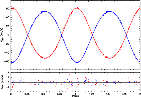
Figure 17: Radial velocities for components A and B of the new triple-lined system KIC 4480321 plotted together with the orbital solution of the inner binary (AB) system and adjusted systemic velocity offsets. The residuals are shown in the bottom part.

7.2 KIC 5219533

From the RV plot, we estimated an orbital period of the order of 32 days and derived a corresponding plausible orbital solution for the inner binary (AB) of this new SB3 system. Our solution confirms the twin character of the inner pair. The orbital parameters are listed in the upper panel of Table 5. Due to the presence of the (diluted) third component which influences the systemic velocity of the inner binary, we allowed for variability of this parameter. Both component RV curves are illustrated in Fig. 18. We find a limitation on the inclination $i$ if we consider that each component of the inner binary should have a mass in the range [1.5 - 3.5] M_⊙ (following the conclusion in Sect. 6.4). We then obtain the condition 46.5 ¡ $i$ ¡ 72$\degr$. A preliminary solution for the systemic radial velocity of the close pair indicates that a period of the order of 1600 days accomodates the current RV data well (see Fig. 3, Appendix B). The parameters of this tentative orbital solution are listed in the bottom panel of Table 5. One data point is an obvious outlier caused by the presence of a blend. Additional RVs are planned to determine a more accurate orbital solution for the AB pair, as well as to better constrain the wide orbit of this system. In Sect. 8, we will present new evidence for the outer orbital solution.

Table 5: Values and standard deviations of the constrained parameters of the orbital solutions for KIC 5219533.

Solution A-B
Orbital parameter	Value			Std. dev.
$P$ (days)	31	.	9181	0	.	0006
$T_{\rm{0}}$ (Hel. JD)	57467	.	41	0	.	04
$e$	0	.	273	0	.	002
$\omega$ (°)	335	.	1	0	.	4
$V_{0}$ (km s-1)	(var.)
$K_{\rm{A}}$ (km s-1)	47	.	1	0	.	4
$K_{\rm{B}}$ (km s-1)	49	.	1	0	.	5
$a_{\rm{A}}\mathrm{sin}\,i$ (AU)	0	.	133	0	.	001
$a_{\rm{B}}\mathrm{sin}\,i$ (AU)	0	.	139	0	.	001
$M_{\rm{A}}\mathrm{sin}\,i^{3}$ (M⊙)	1	.	34	0	.	03
$M_{\rm{B}}\mathrm{sin}\,i^{3}$ (M⊙)	1	.	28	0	.	03
$rms_{\rm{A}}$ (km s-1)	0	.	203
$rms_{\rm{B}}$ (km s-1)	0	.	315
Tentative solution AB-C
Orbital parameter	Value			Std. dev.
$P$ (days)	1595	.		5	.
$T_{\rm{0}}$ (Hel. JD)	58815	.		9	.
$e$	0	.	57	0	.	04
$\omega$ (°)	30	.		4	.
$V_{0}$ (km s-1)	10	.	6	0	.	3
$K_{\rm{AB}}$ (km s-1)	12	.		1	.
$a_{\rm{AB}}\mathrm{sin}\,i$ (AU)	1	.	5	0	.	2
$f(m_{\rm{C}})$ (M⊙)	0	.	19	0	.	08
$rms_{\rm{AB}}$ (km s-1)	0	.	228

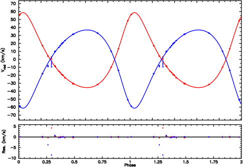
Figure 18: Radial velocities for components A and B of the new triple-lined system KIC 5219533 plotted with a plausible orbital solution for the inner binary (AB) system. The residuals are shown in the bottom part.

7.3 KIC 6381306

We computed the best-fitting orbital period using Period04 and obtained the value of 3.9 days. This value was subsequently refined using the code vcurve_SB for double-lined systems. The presence of the third component influences the systemic velocity of the inner binary, thus we allowed for systematic offsets of its value with time. Both component RV curves are represented in Fig. 19. The residuals are very small and show no systematic trend. The orbital parameters of the close (AB) and the wide (AB-C) system are listed in Table 6. We remark that, since the eccentricity of the AB pair is consistent with null, the orbit is circular, therefore neither $\omega$ nor $T_{\rm{0}}$ are very meaningful. The phased RV curves of the centre of mass of the close pair AB, together with that of of component C, based on an orbital period of 212 days, are displayed in Fig. 4 (Appendix B). We can furthermore derive strict limitations on both inclinations from the condition that each component of this system should have a mass in the range [1 - 3.5] M_⊙ (following the conclusion in Sect. 6.7). We thus obtain the following conditions: 8.5 ¡ $i$ ¡ 13°and 8.4 ¡ $i_{outer}$ ¡ 10°. Note that there is a high probability of co-planarity.

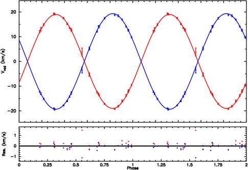
Figure 19: Radial velocities for components A and B of the new triple-lined system KIC 6381306 plotted together with the orbital solution of the inner (AB) binary system and adjusted systemic velocity offsets. The residuals are shown in the bottom part.

Table 6: Values and standard deviations of the constrained parameters of the orbital solutions for KIC 6381306.

Solution A-B
Orbital parameter	Value			Std. dev.
$P$ (days)	3	.	91140	0	.	00001
$T_{\rm{0}}$ (Hel. JD)	56975	.	052	0	.	002
$e$	0	.	001	0	.	002
$\omega$ (°)			—			—
$V_{0}$ (km s-1)	(var.)
$K_{\rm{A}}$ (km s-1)	19	.	00	0	.	07
$K_{\rm{B}}$ (km s-1)	19	.	34	0	.	07
$a_{\rm{A}}\mathrm{sin}\,i$ (AU)	0	.	00683	0	.	00003
$a_{\rm{B}}\mathrm{sin}\,i$ (AU)	0	.	00695	0	.	00002
$M_{\rm{A}}\mathrm{sin}\,i^{3}$ (M⊙)	0	.	01151	0	.	00009
$M_{\rm{B}}\mathrm{sin}\,i^{3}$ (M⊙)	0	.	01131	0	.	00009
$rms_{\rm{A}}$ (km s-1)	0	.	174
$rms_{\rm{B}}$ (km s-1)	0	.	140
Preliminary solution AB-C
Orbital parameter	Value			Std. dev.
$P$ (days)	212	.	0	0	.	3
$T_{\rm{0}}$ (Hel. JD)	57168	.		3	.
$e$	0	.	116	0	.	020
$\omega$ (°)	204	.		5	.
$V_{0}$ (km s-1)	-18	.	32	0	.	04
$K_{\rm{AB}}$ (km s-1)	5	.	02	0	.	06
$K_{\rm{C}}$ (km s-1)	5	.	03	0	.	18
$a_{\rm{AB}}\mathrm{sin}\,i_{out}$ (AU)	0	.	0972	0	.	0012
$a_{\rm{C}}\mathrm{sin}\,i_{out}$ (AU)	0	.	097	0	.	004
$M_{\rm{AB}}\mathrm{sin}\,i_{out}^{3}$ (M⊙)	0	.	0109	0	.	0008
$M_{\rm{C}}\mathrm{sin}\,i_{out}^{3}$ (M⊙)	0	.	0109	0	.	0005
$rms_{\rm{AB}}$ (km s-1)	0	.	123
$rms_{\rm{C}}$ (km s-1)	0	.	691

7.4 KIC 7756853

KIC 7756853 is an SB2 whose spectral lines are mostly blended. We recomputed its radial velocities using synthetic spectra with the parameters of model B (cf. Sect. 6.10) and compared them to the original data set. An orbital solution was derived for both cases. We estimated an orbital period of the order of $\sim$ 100 days based on the RV plot of 14 spectra. A slightly better agreement in terms of root mean squared residuals was found using model B: the mean residuals stay below 1 km s^-1 and are systematically smaller than with model A. We therefore consider that the best choice consists of an A1-type primary with $v\,\mathrm{sin}\,i$₁ = 30 km s^-1 and an A5-type secondary with $v\,\mathrm{sin}\,i$₂ = 60 km s^-1 (model B). The adopted orbital solution is illustrated by Fig. 20. Table 7 lists the corresponding orbital parameters with their uncertainties.

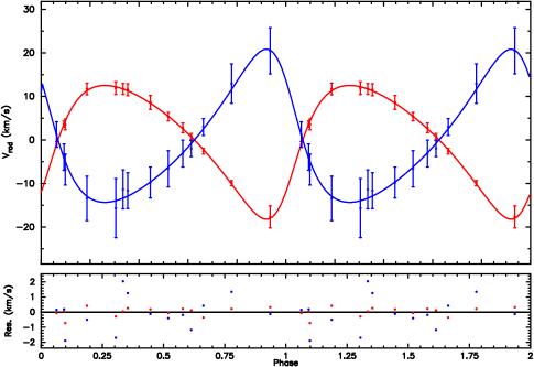
Figure 20: Radial velocities for components A and B of the new double-lined system KIC 7756853 plotted with the proposed orbital solution of the binary. The residuals are shown in the bottom part.

Table 7: Values and standard deviations of the constrained parameters of the orbital solution for KIC 7756853.

Solution A-B
Orbital parameter	Value			Std. dev.
$P$ (days)	99	.	32	0	.	01
$T_{\rm{0}}$ (Hel. JD)	57305	.	8	0	.	5
$e$	0	.	311	0	.	010
$\omega$ (°)	53	.	5	1	.	9
$V_{0}$ (km s-1)	-21	.	51	0	.	13
$K_{\rm{A}}$ (km s-1)	15	.	4	0	.	2
$K_{\rm{B}}$ (km s-1)	17	.	6	0	.	3
$a_{\rm{A}}\mathrm{sin}\,i$ (AU)	0	.	133	0	.	002
$a_{\rm{B}}\mathrm{sin}\,i$ (AU)	0	.	152	0	.	003
$M_{\rm{A}}\mathrm{sin}\,i^{3}$ (M⊙)	0	.	168	0	.	007
$M_{\rm{B}}\mathrm{sin}\,i^{3}$ (M⊙)	0	.	147	0	.	006
$rms_{\rm{A}}$ (km s-1)	0	.	198
$rms_{\rm{B}}$ (km s-1)	0	.	696

7.5 KIC 8975515

The RV curve of the slowly rotating (named secondary) component presents a clearly defined modulation with an amplitude well below 10 km s^-1. From this plot, we estimated an orbital period of the order of 1000 days (possibly longer) for this new SB2 system with dissimilar components. Due to the extreme scatter on the RVs of the fast rotating (named primary) component, we applied the code vcurve_SB for single-lined systems to the data of the secondary (only), and found possible orbital solutions with a period close to either 800 or 1600 days (twice as large). Since the time-delay analysis supports the existence of a 1600-days long variation (cf. Sect. 8), we chose the second possibility. A tentative set of orbital parameters is listed in Table 8. The preliminary orbital solution is illustrated in Fig. 21. It is obvious that this solution accomodates very well the currently available radial velocities of component B since the residuals are really small. In Sect. 8, we will present new evidence to confirm this solution. We will also extend the RV monitoring for another season, in order to further improve the orbital parameters, whilst offering the benefit of a solution of type SB2.

Figure 21: Radial velocities for the companion of KIC 8975515 plotted with the preliminary orbital solution of the binary (type SB1). The residuals are shown in the bottom part.

Table 8: Values and standard deviations of the constrained parameters of the orbital solution for KIC 8975515.

Preliminary solution A-B
Orbital parameter	Value			Std. dev.
$P$ (days)	1582	.		7	.
$T_{\rm{0}}$ (Hel. JD)	57080	.		7	.
$e$	0	.	41	0	.	02
$\omega$ (°)	348	.		2	.
$V_{0}$ (km s-1)	-20	.	47	0	.	07
$K_{\rm{2}}$ (km s-1)	3	.	79	0	.	09
$a_{\rm{2}}\mathrm{sin}\,i$ (AU)	0	.	502	0	.	013
$f(m_{\rm{1}})$ (M⊙)	0	.	0067	0	.	0005
$rms_{\rm{2}}$ (km s-1)	0	.	159

7.6 KIC 9790479

The radial velocity plot of this single-lined system and a preliminary orbital solution based on an approximated period of 231 days are illustrated by Fig. 22. A tentative set of orbital parameters is listed in Table 9.

Figure 22: Radial velocities for the single-lined system KIC 9790479 showing a preliminary orbital solution. The residuals are plotted in the bottom part.

7.7 KIC 11572666

The clearly defined plot for the cooler secondary component of this new SB2 system enabled us to derive an estimated orbital period of 611 days, as well as a tentative set of orbital parameters which is listed in Table 10. This preliminary orbital solution is illustrated in Fig. 23. Due to the huge scatter of the RVs of the primary component, a modelling of type SB2 based on the (weighted) velocities of both components did not allow to improve upon this preliminary solution.

Table 9: Values and standard deviations of the constrained parameters of the orbital solution proposed for KIC 9790479.

Plausible solution A-B
Orbital parameter	Value			Std. dev.
$P$ (days)	230	.	9	0	.	5
$T_{\rm{0}}$ (Hel. JD)	56649	.		9	.
$e$	0	.	24	0	.	03
$\omega$ (°)	76	.		7	.
$V_{0}$ (km s-1)	5	.	2	0	.	3
$K_{\rm{1}}$ (km s-1)	5	.	5	0	.	2
$a_{\rm{1}}\mathrm{sin}\,i$ (AU)	0	.	114	0	.	004
$f(m_{\rm{2}})$ (M⊙)	0	.	0037	0	.	0004
$rms_{\rm{1}}$ (km s-1)	0	.	084

Table 10: Values and standard deviations of the constrained parameters of the orbital solution proposed for KIC 11572666.

Plausible solution A-B
Orbital parameter	Value			Std. dev.
$P$ (days)	611	.		4	.
$T_{\rm{0}}$ (Hel. JD)	57307	.		16	.
$e$	0	.	14	0	.	02
$\omega$ (°)	166	.		9	.
$V_{0}$ (km s-1)	-20	.	2	0	.	1
$K_{\rm{2}}$ (km s-1)	7	.	6	0	.	2
$a_{\rm{2}}\mathrm{sin}\,i$ (AU)	0	.	422	0	.	010
$f(m_{\rm{1}})$ (M⊙)	0	.	0268	0	.	0019
$rms_{\rm{2}}$ (km s-1)	0	.	216

Figure 23: Radial velocities for the companion of KIC 11572666 showing a preliminary orbital solution (type SB1). The residuals are plotted in the bottom part.

8 Time-delay analysis

The orbital motion of a system with a pulsating component introduces a periodic shift of the pulsation frequencies (or their phases) which is caused by variations of the light-travel-time along the orbit. This is known as the ’light-travel-time effect’ (hereafter LiTE). In the case of a multi-mode pulsator, we expect that all the pulsation frequencies show the same cyclical variability pattern. This approach was successfully applied by Murphy et al. (2014) to a sample of $\delta$ Sct stars observed by the Kepler satellite. We applied the same method to the Kepler light curves of all the targets in our sample.

First, we determined all the frequencies with a significance level S/N $>4$ (see e.g. Breger et al. 1993) on the basis of each full data set. Next, we selected the 20 frequencies with the highest S/N. Then, each data set was divided into segments of random length between 9 and 11 days in order to prevent unwanted aliasing. Subsequently, the data of each segment was fitted using a non-linear least-squares fitting routine LCfit (Sódor 2012) with fixed frequencies and starting epoch. In this way, we derived the time-dependent amplitudes and phases for all 20 frequencies. The time delay $\Delta t_{ij}$ for a given frequency $\nu_{j}$ and time segment i is then easily computed using

$$\Delta t_{ij}=\frac{\Delta\phi_{ij}}{2\pi\nu_{j}}$$ (1)

where $\Delta\phi_{ij}$ is the difference between $\phi_{ij}$ and the mean phase calculated from all the segments.

The analysis of the time delays (TDs) is complicated by several factors. Firstly, the phases of the low frequencies (those which might correspond to $\gamma$ Dor frequencies) are often highly scattered, since the corresponding periods are only slightly shorter than the length of the segments and since the frequency spectra often show close peaks that cannot be resolved in the subsets. This is the main reason why we detected correlated phase variations almost exclusively among the higher $\delta$ Sct frequencies. Secondly, some frequencies show significant changes in amplitude and/or phase (usually both) and are thus unstable (Bowman et al. 2016). Such changes will often conceal the overall phase variations caused by LiTE. The analysis can furthermore be affected by the frequency content and distribution. For example, KIC 5965837 shows two most dominant modes with amplitudes of a few mmag in the $\gamma$ Dor regime, while the rest of the frequencies has amplitudes about 30$\times$ lower. In order to reduce the problems with the close frequencies, we also constructed and analysed subsets with a length of 20, 50 and 100 days. Though generally less scattered, these results still remained very close to those of the 10-days long subsets. We adopted the LiTE interpretation as the cause for the detected phase variations when at least three independent frequencies showed the same time-delay pattern.

We discovered correlated variations of comparable amplitude in the time delays of nine objects. In Fig. 24, we illustrate the detection of this effect (LiTE). For the sake of clarity, we show only a few frequencies having the lowest scatter. To highlight the general patterns, we plotted the mean value of five points based on a weighted average computed for 10-days long segments. Whenever the low ($\gamma$-Dor like) frequencies showed some apparent trend, these always followed the trend of the higher ($\delta$-Sct like) frequencies suggesting that both frequency regimes arise in the same star (e.g. f₂ in KIC 9775454). This is also confirmed by the detection of combination peaks of low and high frequencies in the periodograms.

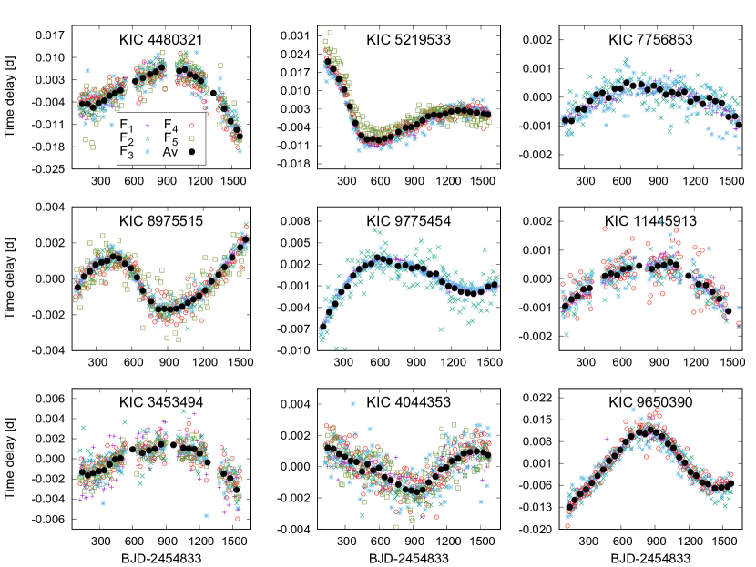
Figure 24: Time delays suggesting orbital motion in nine Kepler candidate hybrid stars. The frequencies are not explicitly listed - their values are listed in Table 12. The symbols and colours in all panels are the same as in the top-left panel. The black circles show the weighted (50 days) averages.

Fig. 24 furthermore shows that the time scales of the detected variations are comparable to the length of the full data sets (i.e. of the order of 4 yrs or longer). In six cases (cf. the upper two rows), RV variability due to orbital motion was also detected (cf. Sect. 7). In three cases (cf. the bottom row), the time delays provide evidence for (undetermined) orbital motions with a long period. However, these targets were classified by us as spectroscopically stable (class ’S’ or ’S?’). It is relevant to note that two of these show extremely broad profiles indicative of very fast rotation which could hamper the detection of spectroscopic multiplicity (KIC 3453494 and 9650390).

In four cases, the LiTE amplitude is large ($\geq 0.01$ days, i.e. KIC 4480321, 5219533, 9775454, and 9650390). In five other cases (three are SB2 systems, e.g. KIC 8975515), the LiTE amplitude is of order of a few thousandths of a day at most. The shortest orbital periods, including 3.9 (KIC 6381306), 9.2 (KIC 4480321), 32 (KIC 5219533), 99 (KIC 7756853) and 212 days (KIC 6381306), were not detected. To increase the chances of detecting the tiny time delays produced by the shortest-period orbits (with an expected total LiTE amplitude of the order of a few $10^{-4}$ days, such as in KIC 6381306 and KIC 4480321), we divided each data set into bins of width 0.10 in orbital phase. We thus obtained ten data sets containing several thousands of points with a time span almost equal to that of the full set for each target. However, even with this modification, the phase variations remained undetected in these two particular cases. This is not due to the method itself, since the smallest LiTE amplitude thus far found in Kepler data equals 8$\cdot 10^{-5}$ days (Murphy et al. 2016a), while the shortest LiTE period yet detected in such light curves is 9.15 days (Murphy et al. 2016b). We conclude that the non-detections may be the consequence of the true LiTE amplitude in combination with the pulsation characteristics of a particular star or system. An alternative and physical explanation is that the detected pulsations might not arise in the close binary itself but in the outer, third component.

In order to show that the detected LiTE has the same cause as the long-term RV variations, we performed a simple modelling based on both data types for the following systems: KIC 4480321, 5219533, and 8975515. We have different orbital solutions for each: KIC 4480321 is a triple-lined system with two SB2 solutions, KIC 5219533 is a triple-lined system with one SB2 and one SB1 solution (for the outer system) while KIC 8975515 is a double-lined system with one SB1 solution (for the slower rotating component). KIC 4480321 AB-C shows the longest detected orbital period (P${}_{orb}\sim$ 2300 d). The inclusion of the time delays allows us to confirm and improve the previous orbital solution. To this purpose, we modelled the TDs adopting the orbital parameters of the RV solution except for the parameter ($a_{C}$. sin $i_{out}$) which was fitted to match the TDs only (cf. Table 11). Fig. 25 shows the excellent agreement between the two data types. The TD residuals in the sense (observed minus modelled) are small and homogeneously distributed around zero. The advantage is a more accurate determination of the mass ratio q_out $\equiv\frac{a_{AB}}{a_{C}}$ = 0.708 $\pm$ 0.004. KIC 5219533 AB-C has P${}_{orb}\sim$ 1600 d. We modelled the TD variations adopting all orbital parameters of the RV solution but fitted an additional parameter ($a_{C}$. sin $i_{out}$) (Table 11). Fig. 26 shows the excellent agreement between the two data types. The TD residuals are small and homogeneously distributed around zero. The advantage is the determination of the new ratio q_out $\equiv\frac{a_{AB}}{a_{C}}$ = 0.56 $\pm$ 0.07. KIC 8975515 AB also has P${}_{orb}\sim$ 1600 d. We modelled the TD variations adopting all orbital parameters of the RV solution but fitted an additional parameter ($a_{A}$. sin $i$) (Table 11). Fig. 27 shows the good agreement between the two data types. The TD residuals are small though somewhat inhomogeneously distributed around zero, as they show a small discrepancy in eccentricity. The advantage here also is the determination of the new ratio q $\equiv\frac{a_{A}}{a_{B}}$ = 0.81 $\pm$ 0.01. In all three cases, we confirm that the observed TDs are consistent with the previously derived RV orbital solutions.

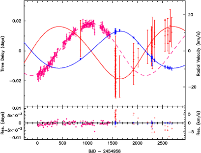
Figure 25: LiTE versus RV orbital solution for KIC 4480321. Note that the TDs (pink symbols) were corrected by removing a linear trend from the original data. The blue and red solid lines refer to the RV solution (see Fig. 2). The dashed line shows the computed model.

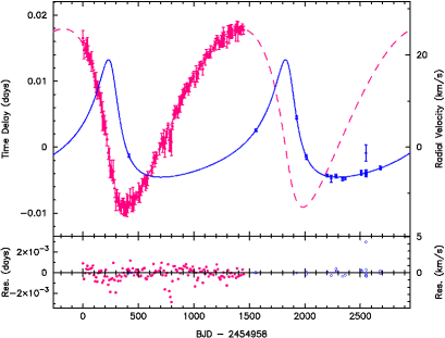
Figure 26: LiTE versus RV orbital motion for KIC 5219533. Note that the TDs (pink symbols) were corrected by removing a linear trend from the original data. The solid line refers to the RV solution (see Fig. 3). The dashed line shows the computed model.

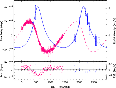
Figure 27: LiTE versus RV orbital motion for KIC 8975515. Note that the TDs (pink symbols) were corrected by removing a linear trend from the original data. The solid line refers to the RV solution (see Fig. 21). The dashed line shows the computed model.

Table 11: Results of a fit of the LiTE adopting the previously derived RV orbital solutions.

KIC Nr	Fitted parameter	Value	Uncertainty
4480321	$a_{C}$ sin $i_{out}$	3.023	0.058
5219533	$a_{C}$ sin $i_{out}$	2.682	0.026
8975515	$a_{A}$ sin $i$	0.4055	0.0036

Such examples illustrate that the TD method can identify long-term changes which nicely complement the results of the spectroscopic analyses. Although the argument for long-term variations caused by orbital motion is quite strong, we should not exclude the possibility that the parabola-shaped variations of the TDs as e.g. observed in KIC 7756853 might also be caused by some intrinsic evolutionary effect. Indeed, such a behaviour was reported in the $\delta$ Sct star 4 CVn. Although 4 CVn is also a short-period spectroscopic binary system (Schmid et al. 2014), the secular variations detected in (only) some pulsation modes follow different patterns related to a change of the rotational splitting (Breger 2016). In the case of the above discussed Kepler stars, however, the reported patterns of the secular variations are common to all investigated frequencies.

Table 12: Frequencies (expressed in d^-1) for which the time delay is plotted in Fig. 24.

KIC Nr	$F_{1}$	$F_{2}$	$F_{3}$	$F_{4}$	$F_{5}$
3453494	7.4989	9.9099	19.6236	16.4034	24.8482
4044353	17.8971	17.1562	21.7553	19.2751	27.5050
4480321	23.0027	14.9304	13.9569	22.9501	13.0734
5219533	10.2853	17.1820	13.2421	15.1066	19.4854
7756853	21.1416	20.7177	18.9791	22.3150
8975515	13.9724	16.0763	17.7345	15.5147
9650390	17.3726	16.3018	12.8837	14.3490
9775454	14.9387	4.6108	14.7482
11445913	31.5579	25.3771	22.1331

9 An observational H-R diagram

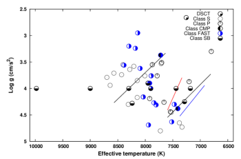
Figure 28: A ($T_{\mathrm{eff}}$, $\mathrm{log}\,g$)-representation for the 50 candidate hybrid stars and one evolved $\delta$ Scuti star. We show the location of the objects belonging to the classes S, P(+VAR), CMP and SB, as well as the rapidly rotating ones (FAST). The empirical borders of the classical $\delta$ Scuti (in black) and $\gamma$ Dor (in colour) instability strips are represented by solid lines.

In Fig. 28, we plotted the distribution of the updated atmospheric parameters for our sample of A/F-type candidate hybrid stars. In this observational ($T_{\mathrm{eff}}$, $\mathrm{log}\,g$)-diagram, we represented the five categories of our classification using different symbols. Based on the new $v\,\mathrm{sin}\,i$ measurements, we furthermore indicated the objects which are subject to (very) fast rotation (i.e. with $v\,\mathrm{sin}\,i$ ¿ 200 km s^-1). Of course, both CMP-targets are fast rotators. The borders of the classical $\delta$ Scuti and the $\gamma$ Doradus instability strips reproduced by Uytterhoeven et al. (2011) are also shown. It is remarkable that all the P-targets are located within these limits. The SB objects located (far) outside the instability strips are KIC 6381306 ($T_{\mathrm{eff}}$ = 9000 K) and KIC 7756853 ($T_{\mathrm{eff}}$ = 9980 K).

10 Discussion and conclusions

We classified a sample of 50 regularly observed bright A/F-type candidate hybrid stars and one $\delta$ Scuti star of the Kepler mission into different classes according to the shape (in some cases, the model) of their cross-correlation profiles and the evolution of their radial velocities with time. Classes were defined as S (for stable), SB (for spectroscopic binary or triple system), VAR (for long-term radial-velocity variable star), P (for pulsating and/or rotating), and CMP (for composite spectrum). According to these spectroscopic criteria, we find the following distribution (without considering the cool object KIC 9700679 which is also SB1): 49% of S-stars, 22% of P-stars, 18% of SB-objects, 6% of VAR-stars and 4% of CMP-objects (Fig. 29). In addition, the VAR-stars are (most) probably long-period SB1 systems. Including the known eclipsing binary KIC 11180361 (KOI-971), we find a global multiplicity fraction of 27%. This indicates that at least 25% of our sample of potential hybrid stars belongs to a binary or a multiple system.

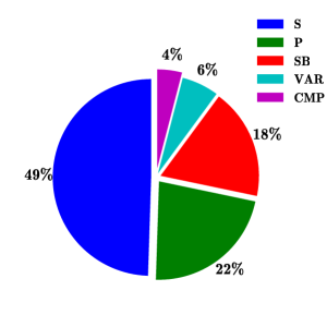
Figure 29: Classification results of the A/F-type candidate hybrid stars.

We (re)determined the fundamental atmospheric properties such as $T_{\mathrm{eff}}$, $\mathrm{log}\,g$ and $v\,\mathrm{sin}\,i$ based on the high-resolution Hermes spectra, which are important physical parameters, for all of our targets including - where feasible - for the components of the newly detected systems. A comparison with the published data showed that our values agree in most cases, though some evident discrepancies were also reported. Evidently, in the case of the multiple systems where the ambiguity is higher, several possible models were found. In these cases, we usually adopted the solution from the [500 - 520] nm interval. Consequently, we presented an updated observational H-R diagram.

At this stage, we can start to address our longer term goal by taking a closer look at the frequency content of the newly reported systems in the region of interest, i.e. in the $\gamma$ Dor regime. In Fig. 30, we present the periodograms in the low-frequency range, i.e. [0-4] d^-1, based on the Kepler data sets for the seven spectroscopic (binary and multiple) systems discussed in Sect. 7. The aim is to search for the presence of the orbital frequencies in the original periodograms. We see that, in most cases, the amplitudes in the vicinity of the orbital frequency are either much lower than the amplitudes of the obvious peaks or fully embedded in the noise. There are two exceptions, however: KIC 4480321 and 6381306. In the case of KIC 4480321 (SB3), which shows the highest power in the explored range, there is a well-detected peak (with an amplitude of 0.04 parts per thousand (ppt)) which is close though not identical to the orbital frequency. In the case of KIC 6381306 (SB3), the dominant peak (with an amplitude of 0.1 ppt) agrees perfectly with the spectroscopically derived orbital frequency. In all other cases, we can find no clear sign of the presence of the orbital frequency in the periodograms. The figure furthermore demonstrates that all these systems are rather strongly multi-periodic in the low-frequency regime.

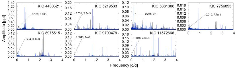
Figure 30: Periodograms of the Kepler light curves for the seven SB systems discussed in Sect. 7. For each object, the position corresponding to the newly revealed orbital frequency is plotted as a dashed line indicated by an arrow, and the frequency value as well as its amplitude (expressed in relative intensity units) are mentioned.

We also searched for regular frequency spacings in the full-scale periodograms of these objects which might be linked to the orbital frequency. In an eccentric binary system, the tidal potential can indeed be represented by a Fourier series with many forcing frequencies. When one of the forcing frequencies happens to be close to an eigenfrequency, the oscillation mode is resonantly excited (tidally induced) (Willems 2003). A well-known example of detected tidal excitation is the Kepler main-sequence binary KOI-54, where the strongest oscillations occur at 90 and 91 times the orbital frequency (Fuller & Lai 2012). Table 13 lists the relevant spacings for each target. In Fig. 31, we plotted the frequency spacings in the range [0-4] d^-1 on a logarithmic scale for the SB systems discussed in Sect. 7. We see that KIC 4480321 has the most dominant and most densely distributed spacing pattern. In comparison, the spacing density of the other systems is very poor. In the case of KIC 4480321, the most frequent spacing (S₁ = 0.0085 d ^-1) corresponds to the exact difference of the next two most frequent ones, i.e. 0.0928 and 0.1013 d^-1, which are both very close but not equal to the orbital frequency (0.1091 d^-1). We conclude that this signals the influence of the orbital frequency of the close (AB) pair on the other frequencies of KIC 4480321. In the case of KIC 6381306, we highlight the presence of a single significant spacing in this range (S₁ = 1.3355 d^-1).

Table 13: Most relevant frequency spacings (expressed in d^-1) sorted according to decreasing importance for the SB systems of Sect. 7.

KIC Nr	$S_{1}$	$S_{2}$	$S_{3}$	$S_{4}$	$S_{5}$
4480321	0.0085	0.0928	0.1013	0.0787	0.0872
5219533	8.6315	8.5682	0.0632	5.9755	8.8068
6381306	1.3355	5.5596	5.0208	4.7808	4.4781
7756853	0.4240	2.1626	20.2503	15.4084	–
8975515	11.5981	11.6622	11.4488	0.0641	0.1493
9790479	0.0217	1.2210	0.9324	10.3974	0.7654
11572666	16.3120	1.9671	15.8459	14.7212	10.9377

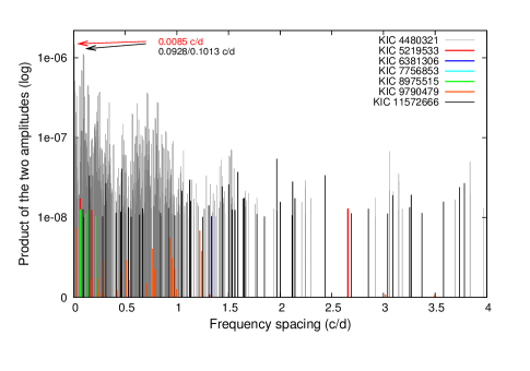
Figure 31: Frequency spacings for the SB systems discussed in Sect. 7. The weights (plotted on the Y-axis) were computed as the product of the amplitudes of both frequencies. For each object, a different colour is used. KIC 4480321 presents by far the richest spacing pattern. Its dominant spacings are located in the vicinity of the orbital frequency. The arrows indicate two of the most frequent spacings as well as their difference.

This study represents an unavoidable step in the investigation of the new A/F-type hybrid phenomenon. We find a significant rate of both short- and long-period binary/multiple systems among our targets. The multiplicity comes with different flavours. If we add the positive new detections from the photometric time-delay analysis, we may include the targets KIC 3453494, 4044353 and 9650390 as (most probably) belonging to the class of single-lined, long-period binary systems. The multi-year monitoring of the RVs enabled the detection of several long-period systems with orbital periods of the order of 4-6 years, e.g. KIC 4480321, 5219533, 8975515 and 9775454. It is our intention to continue the monitoring for these interesting systems. Moreover, since the photometric time-delay analysis - which is based on the 4-years time span of the Kepler mission - shows the existence of periodicities of the same order, we intend to combine both data types into a simultaneous modelling in the near future. Indeed, we already showed that the orbital solutions currently based on the RVs only are confirmed by a simple modelling of the LiTE in three cases. Overall, we may safely conclude that about one third of our sample of candidate hybrid stars belongs to a binary or a multiple system. This number is very close to the fraction of binary and multiple systems suggested from a spectroscopic-photometric analysis for a sample of 32 candidate SX Phe stars in the Kepler field (Nemec et al. 2017).

This result implies that the physical cause of the low frequencies which are detected in the Kepler periodograms could be related to the orbital motions, and that these so-called hybrid stars may not be genuine hybrid pulsators. They may have forced oscillations coupled to the orbital frequency (its harmonics), or show ellipsoidal modulations in their light curves. In two of the seven SB systems, we found straightforward evidence for the presence of the orbital frequency in the periodograms (KIC 4480321 and 6381306). In KIC 6381306, the orbital frequency is the most dominant peak. It is worth noting that such interaction was detected in the two short-period systems with an orbital period smaller than 10 d. In the remaining cases (those with orbital periods beyond 30 d), there is no influence at first sight, the more dominant peaks are situated in the range [0.5-3] d^-1, as is usual for the g-mode pulsators of $\gamma$ Dor type. The multiperiodicity and apparent complexity of the frequency content in this region still need an explanation in most of the (long-period) systems.

We are not yet able to differentiate between the true hybrid pulsators and those stars where spots or fast rotation introduce inhomogeneities on the stellar surface. On the one hand, an extended analysis of the Kepler data including a precise identification of the g-mode period spacing patterns may help out, provided there are enough visible g-modes to reliably detect such patterns (e.g. Van Reeth et al. 2015). On the other hand, detailed spectropolarimetric investigations (e.g. Neiner & Lampens 2015) can provide true physical insight regarding the origin of the low frequencies in some cases. In conclusion, the resulting orbital periods and elements of the newly identified systems, projected rotational velocities and homogeneous atmospheric properties provide relevant and essential information for a more reliable and deeper physical understanding of the Kepler periodograms.

Appendix A Cross-correlation functions of A/F-type candidate hybrid stars

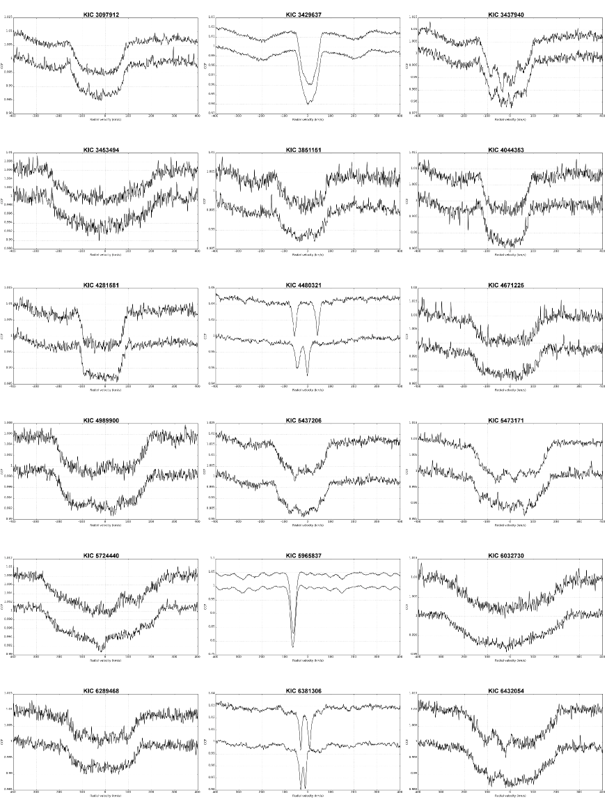
Figure 32: Cross-correlation functions for 48 Kepler objects. The epochs were chosen so as to show as much contrast as possible between two CCFs.

Appendix B Radial velocity curves

Figure 1: Radial velocity plots for 44 Kepler objects (cont’ed). The same symbols as before are used.

Figure 1: Radial velocity plots for 44 Kepler objects (cont’ed). The same symbols as before are used.

Figure 3: Radial velocities for the mass centre of the inner binary (AB) in the triple system KIC 5219533 plotted over a tentative orbital solution with a period of about 1600 days. The residuals are shown in the bottom part.

Appendix C List of radial velocity data

Table 1: List of radial velocity data used in this work. I. Single objects and single-lined systems. H stands for Hermes while A stands for Ace.

KIC	HJD	RV1	$\sigma_{RV_{1}}$	Source
Nr		km s-1	km s-1	[1:H, 2:A]
3097912	2455311.54168	-28.232	2.894	1
3097912	2455311.56259	-28.092	4.071	1
3097912	2456970.40110	-27.605	2.986	1
3097912	2456973.30681	-27.623	3.353	1
3097912	2457150.67141	-25.497	4.127	1
3429637	2456394.66396	5.312	0.907	1
3429637	2456395.69257	5.023	0.889	1
3429637	2456395.69610	5.050	1.157	1
3429637	2456396.71561	5.016	0.977	1
3429637	2456397.70470	4.908	0.916	1
3429637	2456400.67080	5.483	1.079	1
3429637	2456400.67590	5.249	0.961	1
3429637	2456404.65240	5.015	1.092	1
3429637	2456515.59496	6.703	0.935	1
3429637	2456515.59971	6.546	1.109	1
3429637	2456516.55962	6.521	0.983	1
3429637	2456516.56367	6.599	1.028	1
3429637	2456518.57790	6.426	1.034	1
3429637	2456518.58219	6.617	0.848	1
3429637	2457150.67944	5.517	0.905	1
3429637	2457240.53988	8.049	1.047	1
3429637	2457240.54300	7.826	1.004	1
3429637	2457508.64772	5.221	0.983	1
3429637	2457512.68770	4.652	0.963	1
3429637	2457542.67355	4.456	1.009	1
3429637	2457546.68561	4.971	1.025	1
3437940	2456772.71163	-14.391	3.929	1
3437940	2456778.66784	-14.772	2.999	1
3437940	2456797.70882	-15.188	2.868	1
3437940	2456818.49499	-15.224	3.575	1
3437940	2456883.55172	-14.632	3.248	1
3437940	2456967.41540	-14.520	3.273	1
3437940	2456968.39509	-14.901	3.352	1
3437940	2456961.35130	-17.167	7.365	2
3437940	2456961.36185	-16.081	8.441	2
3437940	2457101.64638	-12.634	2.722	2
3437940	2457101.65346	-14.081	5.820	2
3453494	2456774.65266	-11.613	14.896	1
3453494	2456780.57524	-10.767	8.262	1
3453494	2456811.68040	-11.570	9.430	1
3453494	2456821.68229	-12.931	13.539	1
3453494	2456822.53636	-12.086	8.251	1
3851151	2455379.67069	-19.094	2.882	1
3851151	2456776.62228	-20.211	4.168	1
3851151	2456782.70247	-20.018	4.192	1
3851151	2456811.62472	-20.307	4.655	1
3851151	2456820.53335	-21.031	4.989	1
4044353	2455376.40432	-19.168	2.209	1
4044353	2455427.46872	-19.510	2.947	1
4044353	2456973.33836	-18.771	4.039	1
4044353	2457152.59995	-19.027	3.340	1
4044353	2457160.71443	-18.238	1.733	1
4044353	2457168.68652	-19.214	2.406	1
4281581	2455756.43195	-12.806	1.908	1
4281581	2456776.71295	-13.327	1.796	1
4281581	2456782.72081	-13.743	1.569	1
4281581	2456811.72924	-12.094	1.966	1
4281581	2456822.62333	-12.869	1.947	1
4671225	2455823.57267	-13.770	3.156	1

Table 1: List of radial velocity data obtained in this work (cont’ed).

KIC	HJD	RV1	$\sigma_{RV_{1}}$	Source
Nr		km s-1	km s-1	[1:H, 2:A]
4671225	2455823.59410	-15.743	5.634	1
4671225	2456778.64304	-13.057	4.099	1
4671225	2456783.60829	-12.604	4.422	1
4671225	2456811.70493	-13.257	5.286	1
4671225	2456822.61118	-14.156	5.508	1
4989900	2456772.64609	-12.981	6.090	1
4989900	2456778.60890	-14.227	4.681	1
4989900	2456805.54342	-13.037	4.341	1
4989900	2456817.46014	-13.580	4.399	1
4989900	2457237.48797	-13.690	4.535	1
4989900	2456967.29285	-16.728	10.288	2
4989900	2456967.29993	-16.525	7.052	2
4989900	2457101.60021	-13.380	20.922	2
4989900	2457101.60430	-15.485	21.511	2
5437206	2456773.66428	-27.617	2.172	1
5437206	2456779.65943	-26.971	2.501	1
5437206	2456810.71459	-26.634	2.606	1
5437206	2456817.53064	-27.151	2.574	1
5437206	2456883.58181	-27.334	2.246	1
5437206	2456968.38919	-27.258	2.299	1
5437206	2456961.33016	-30.586	5.466	2
5437206	2456961.33800	-25.908	8.516	2
5437206	2456967.26422	-26.901	4.145	2
5437206	2456967.27476	-26.172	6.463	2
5437206	2457101.63125	-26.220	6.934	2
5437206	2457101.63833	-28.619	5.402	2
5473171	2455346.71377	5.768	4.140	1
5473171	2455428.60548	6.175	4.168	1
5473171	2456972.42132	6.794	3.000	1
5473171	2457152.73117	8.031	4.340	1
5473171	2457160.58231	6.643	3.611	1
5724440	2455754.62168	-16.766	11.095	1
5724440	2456776.60161	-15.549	8.651	1
5724440	2456782.73249	-17.067	11.227	1
5724440	2456804.69937	-15.408	11.233	1
5724440	2456818.59991	-15.034	8.127	1
5724440	2457641.35795	-13.547	8.842	1
5724440	2457642.43018	-18.419	10.997	1
5724440	2456975.25240	-27.856	14.415	2
5724440	2457102.59934	-25.953	19.935	2
5724440	2457102.60988	-25.700	12.292	2
5965837	2456773.72880	-65.089	0.297	1
5965837	2456779.70476	-65.513	0.294	1
5965837	2456811.67010	-63.839	0.277	1
5965837	2456821.57179	-63.050	0.274	1
5965837	2456883.58903	-64.065	0.248	1
5965837	2456969.42152	-63.523	0.287	1
5965837	2456974.36215	-64.155	0.291	1
5965837	2456961.44476	-64.476	0.686	2
5965837	2457105.59866	-63.127	0.683	2
5965837	2457105.61269	-63.239	0.276	2
6032730	2455754.63578	-13.302	7.483	1
6032730	2456775.59004	-12.343	14.577	1
6032730	2456781.56291	-12.300	9.119	1
6032730	2456797.70282	-11.784	9.352	1
6032730	2456817.49621	-13.497	10.418	1
6289468	2456773.71476	-6.096	5.940	1
6289468	2456779.68743	-6.148	7.381	1
6289468	2456811.66097	-5.215	6.681	1

Table 1: List of radial velocity data obtained in this work (cont’ed).

KIC	HJD	RV1	$\sigma_{RV_{1}}$	Source
Nr		km s-1	km s-1	[1:H, 2:A]
6289468	2456820.50998	-6.006	7.884	1
6289468	2457160.62559	-6.491	8.570	1
6289468	2457238.40678	-7.420	7.749	1
6289468	2457241.57072	-6.086	6.765	1
6432054	2456772.68105	12.487	4.117	1
6432054	2456778.66024	11.371	3.466	1
6432054	2456808.72721	14.375	4.164	1
6432054	2456817.46483	14.141	5.659	1
6432054	2456937.33008	13.007	5.836	1
6432054	2457237.53342	12.296	3.471	1
6432054	2457102.66971	11.450	5.618	2
6432054	2457105.57294	8.609	8.813	2
6432054	2457105.58350	8.167	11.919	2
6587551	2455324.60504	-11.161	5.647	1
6587551	2455375.45092	-9.659	5.523	1
6587551	2455426.51924	-8.506	3.624	1
6587551	2456973.32091	-9.805	4.653	1
6670742	2456773.61170	-23.321	12.241	1
6670742	2456779.61973	-24.514	12.799	1
6670742	2456805.54978	-25.477	10.960	1
6670742	2456818.47289	-28.333	14.159	1
6670742	2456883.60322	-19.881	15.810	1
6670742	2456938.32442	-24.783	12.612	1
6670742	2456970.35905	-21.691	12.548	1
6756386	2455288.62548	-31.702	7.117	1
6756386	2455288.67489	-33.885	5.450	1
6756386	2455426.49828	-32.975	6.378	1
6756386	2456881.45976	-20.393	4.830	1
6756386	2456971.38273	-37.117	4.604	1
6756386	2457150.66253	-18.489	7.270	1
6756386	2457166.53003	-23.779	7.387	1
6756481	2455315.53247	-24.024	9.882	1
6756481	2455315.55886	-20.659	14.441	1
6756481	2456772.66149	-26.604	11.409	1
6756481	2456779.59133	-27.550	11.607	1
6756481	2456798.56487	-25.852	10.112	1
6756481	2456818.46355	-29.137	11.630	1
6756481	2457237.49645	-29.619	10.804	1
6951642	2455820.49393	-4.548	3.288	1
6951642	2455820.51536	-4.498	3.086	1
6951642	2455823.51759	-4.914	2.701	1
6951642	2455823.53555	-4.329	2.926	1
6951642	2456515.56384	-0.513	2.731	1
6951642	2456515.57600	-0.875	2.514	1
6951642	2456601.32535	-1.193	2.373	1
6951642	2456605.33444	0.268	3.867	1
6951642	2456605.34196	-0.334	4.113	1
6951642	2457512.66815	-2.463	2.011	1
6951642	2457514.52780	-2.946	2.257	1
7119530	2455347.57120	-25.084	9.969	1
7119530	2455428.47331	-26.335	10.227	1
7119530	2456772.72645	-24.769	8.836	1
7119530	2456778.71894	-22.745	11.450	1
7119530	2456810.71977	-22.995	8.135	1
7119530	2456818.50025	-24.642	9.132	1
7119530	2457154.68125	-25.826	8.913	1
7668791	2456773.62219	-28.170	0.663	1
7668791	2456778.73062	-27.987	0.763	1
7668791	2456808.51473	-28.117	1.031	1

Table 1: List of radial velocity data obtained in this work (cont’ed).

KIC	HJD	RV1	$\sigma_{RV_{1}}$	Source
Nr		km s-1	km s-1	[1:H, 2:A]
7668791	2456818.48741	-28.210	0.629	1
7668791	2456883.61216	-27.888	0.714	1
7668791	2456938.34404	-28.299	0.721	1
7668791	2456971.39724	-27.982	0.762	1
7748238	2456773.67912	-20.810	4.052	1
7748238	2456778.68018	-22.638	3.651	1
7748238	2456797.71653	-21.253	3.391	1
7748238	2456820.46554	-21.850	3.712	1
7748238	2456883.62187	-21.259	4.082	1
7748238	2456970.41652	-22.071	3.188	1
7770282	2455757.55581	7.995	1.190	1
7770282	2456774.69850	6.867	0.938	1
7770282	2456780.61058	6.907	0.982	1
7770282	2456811.71804	0.321	0.735	1
7770282	2456822.63350	10.340	0.863	1
7770282	2456886.45275	7.288	1.060	1
7770282	2456968.35190	7.980	0.769	1
7770282	2456973.43099	5.635	0.983	1
7770282	2457160.68386	6.613	0.924	1
7770282	2457239.49784	6.594	0.895	1
7770282	2457241.62622	6.521	1.162	1
7770282	2457244.64261	7.518	1.004	1
7770282	2457250.59059	8.367	0.728	1
7770282	2457253.51929	7.643	0.597	1
7770282	2457254.51474	8.566	0.741	1
7770282	2457267.44587	6.348	0.919	1
7770282	2457303.45019	8.443	1.100	1
7770282	2457314.34908	8.862	0.681	1
7770282	2457510.68143	8.251	0.738	1
7770282	2457515.65056	7.400	1.029	1
7827131	2456772.73822	-29.626	19.897	1
7827131	2456778.61547	-31.674	18.869	1
7827131	2456810.70891	-35.339	26.093	1
7827131	2456820.60947	-31.831	24.875	1
7827131	2456975.32256	-62.103	33.058	2
7827131	2456976.28539	-49.278	41.536	2
7827131	2456976.30289	-47.238	31.700	2
7827131	2457102.62711	-34.005	23.223	2
7827131	2457102.63765	-31.850	36.118	2
7959867	2455429.45817	-18.069	5.575	1
7959867	2455429.48421	-17.516	4.631	1
7959867	2456778.58412	-21.501	3.563	1
7959867	2456783.72252	-22.566	3.299	1
7959867	2456811.63763	-22.867	5.364	1
7959867	2456821.55056	-21.496	4.861	1
8738244	2456773.60399	6.219	3.733	1
8738244	2456779.64298	6.742	2.821	1
8738244	2456798.57186	8.232	3.732	1
8738244	2456818.47999	5.844	4.291	1
8738244	2457237.50518	6.023	3.562	1
8738244	2457105.62750	9.017	5.215	2
8738244	2457105.63948	10.760	13.121	2
8915335	2455825.60788	-13.917	6.737	1
8915335	2455835.52742	-13.817	4.307	1
8915335	2456970.43273	-13.421	8.489	1
8915335	2456972.43264	-10.682	5.419	1
8915335	2457159.72063	-12.448	6.870	1
8915335	2457189.69417	-12.846	5.294	1
9351622	2455754.73591	-7.794	1.798	1

Table 1: List of radial velocity data obtained in this work (cont’ed).

KIC	HJD	RV1	$\sigma_{RV_{1}}$	Source
Nr		km s-1	km s-1	[1:H, 2:A]
9351622	2456773.74009	-7.317	1.415	1
9351622	2456778.70867	-7.010	1.620	1
9351622	2456810.72603	-7.512	1.566	1
9351622	2456822.59921	-7.728	1.519	1
9351622	2456886.46224	-7.195	1.860	1
9351622	2456971.42319	-7.795	2.076	1
9351622	2456974.39870	-7.926	1.474	1
9351622	2457152.64337	-7.738	1.624	1
9413057	2456774.67389	3.898	6.966	1
9413057	2456780.59142	1.254	7.805	1
9413057	2456811.69127	4.591	8.140	1
9413057	2456822.58947	5.216	7.719	1
9509296	2456123.42703	1.648	2.478	1
9509296	2456174.47840	1.794	2.545	1
9509296	2456174.49981	0.800	3.051	1
9509296	2456881.44520	2.167	2.167	1
9509296	2456970.37567	0.763	3.186	1
9509296	2457153.58330	0.209	3.375	1
9509296	2457161.66127	-0.186	2.494	1
9509296	2457189.51292	1.196	2.344	1
9650390	2456773.69836	-2.863	17.528	1
9650390	2456778.69577	2.884	21.984	1
9650390	2456797.72640	-2.476	23.540	1
9650390	2456821.56189	-3.322	17.283	1
9650390	2456886.47090	0.527	20.850	1
9650390	2456937.46750	-5.435	23.806	1
9650390	2456971.41076	-4.444	23.526	1
9700679	2455757.43749	-3.201	0.111	1
9700679	2457241.47140	-5.474	0.122	1
9700679	2457640.43617	-6.314	0.169	1
9700679	2457646.41875	-6.373	0.107	1
9764965	2455352.65996	-22.759	1.493	1
9764965	2455424.48352	-22.921	1.802	1
9764965	2456972.36986	-23.213	1.534	1
9764965	2457151.63879	-23.031	1.843	1
9764965	2457239.58872	-23.006	1.640	1
9764965	2457240.65141	-22.236	2.079	1
9775454	2455345.73254	-21.715	1.206	1
9775454	2455351.63147	-21.844	1.197	1
9775454	2455424.57568	-23.147	1.508	1
9775454	2456969.38823	-20.252	1.208	1
9775454	2456974.38906	-20.053	1.225	1
9775454	2457159.56449	-24.129	1.525	1
9775454	2457238.61841	-24.978	1.060	1
9775454	2457240.69656	-24.915	1.428	1
9775454	2457302.48479	-25.854	1.209	1
9775454	2457314.39042	-25.471	1.310	1
9775454	2457508.70996	-26.797	1.414	1
9775454	2457514.54436	-26.693	1.342	1
9775454	2457548.70096	-26.976	1.268	1
9790479	2456774.72513	5.098	0.660	1
9790479	2456781.62401	4.462	0.629	1
9790479	2456809.70861	1.582	0.732	1
9790479	2456822.71439	0.820	0.709	1
9790479	2456940.47525	10.116	0.578	1
9790479	2456940.49041	10.141	0.682	1
9790479	2457160.64783	10.401	0.573	1
9790479	2457239.57310	4.877	0.754	1
9790479	2457241.64648	4.909	0.856	1

Table 1: List of radial velocity data obtained in this work (cont’ed).

KIC	HJD	RV1	$\sigma_{RV_{1}}$	Source
Nr		km s-1	km s-1	[1:H, 2:A]
9790479	2457298.49499	-0.441	0.776	1
9790479	2457515.68719	0.345	0.970	1
9970568	2455756.69520	9.880	7.754	1
9970568	2456776.73133	11.896	11.861	1
9970568	2456781.71387	8.834	7.530	1
9970568	2456809.72125	9.053	7.642	1
9970568	2456820.62195	10.306	8.293	1
10264728	2456123.45722	-23.684	10.467	1
10264728	2456182.45512	-22.298	8.008	1
10264728	2456182.47654	-23.584	10.603	1
10264728	2457151.62153	-21.205	10.801	1
10537907	2455471.41011	1.223	3.031	1
10537907	2456971.44393	-4.202	2.921	1
10537907	2457151.65012	-5.109	3.582	1
10537907	2457168.69958	-4.960	3.995	1
10537907	2457638.46798	-3.837	1.972	1
10537907	2457646.40239	-2.315	3.624	1
10664975	2456772.69135	10.799	6.442	1
10664975	2456772.69864	12.437	7.265	1
10664975	2456778.62709	11.848	5.786	1
10664975	2456810.70401	10.119	7.299	1
10664975	2456820.47253	12.419	7.715	1
10664975	2456937.32218	6.643	7.950	1
10664975	2456967.31888	2.786	24.771	2
10664975	2456976.36798	-25.089	42.789	2
10664975	2457101.61319	-0.566	41.508	2
10664975	2457101.62051	6.745	35.514	2
11180361	2455754.57653	-19.707	4.609	1
11180361	2456969.37347	-17.525	5.630	1
11180361	2456972.41405	-20.884	6.264	1
11180361	2457151.63197	-20.212	5.272	1
11180361	2457166.53519	-20.334	3.966	1
11180361	2457238.58629	-19.588	4.808	1
11180361	2457240.54658	-20.504	4.576	1
11193046	2455756.65596	4.393	6.674	1
11193046	2456775.61353	5.088	8.089	1
11193046	2456780.55660	1.821	6.008	1
11193046	2456811.64969	3.939	7.406	1
11193046	2456820.52000	5.767	8.288	1
11602449	2455375.53821	-3.965	3.780	1
11602449	2456513.44363	-4.035	3.446	1
11602449	2456513.45810	-6.444	4.019	1
11602449	2456516.44907	-2.959	3.270	1
11602449	2456516.46470	-4.486	2.788	1
11602449	2456516.59601	-5.784	4.120	1
11602449	2456516.61048	-2.441	2.689	1
11602449	2456521.51360	-3.152	3.859	1
11602449	2456521.53270	-4.629	3.073	1
11602449	2456522.44959	-5.080	2.636	1
11602449	2456523.41676	-4.925	3.885	1
11602449	2456523.43586	-0.728	5.334	1
11602449	2456523.60775	-4.268	4.199	1
11602449	2456523.62685	-3.934	6.182	1

Table 2: List of radial velocity data used in this work. II. Double- and triple-lined systems. H stands for Hermes while A stands for Ace.

KIC	HJD	RV1	$\sigma_{RV_{1}}$	RV2	$\sigma_{RV_{2}}$	RV3	$\sigma_{RV_{3}}$	Source
Nr		km s-1	km s-1	km s-1	km s-1	km s-1	km s-1	[1:H, 2:A]
4480321	2455820.44990	-45.392	0.408	-3.146	0.352	-12.481	10.101	1
4480321	2455820.47133	-45.885	0.548	-2.540	0.272	-11.552	7.182	1
4480321	2456513.50147	40.447	0.487	-61.375	0.409	-28.157	6.368	1
4480321	2456513.51999	41.381	0.535	-61.823	0.298	-28.192	9.238	1
4480321	2456513.65562	44.472	0.458	-64.841	0.365	-30.583	8.740	1
4480321	2456513.67472	44.602	0.526	-64.910	0.453	-31.058	13.289	1
4480321	2456515.50195	30.270	0.372	-46.044	0.421	-29.535	8.923	1
4480321	2456515.51873	29.923	0.393	-45.714	0.289	-32.465	7.798	1
4480321	2456515.63327	25.284	0.308	-41.175	0.348	-30.446	10.021	1
4480321	2456515.65352	24.614	0.349	-40.367	0.737	-28.934	9.367	1
4480321	2456518.46971	-59.149	1.759	43.292	1.457	–	–	1
4480321	2456518.48186	-59.665	0.684	42.940	1.183	-27.161	16.127	1
4480321	2456518.59682	-60.045	0.517	43.882	0.507	-31.598	7.543	1
4480321	2456518.61708	-60.169	0.841	43.828	0.726	-30.313	12.504	1
4480321	2456519.49085	-58.282	0.466	41.799	0.462	-33.559	8.221	1
4480321	2456519.50994	-58.188	0.323	41.351	0.417	-36.208	5.361	1
4480321	2456519.65219	-56.046	0.373	39.399	0.285	-33.468	11.277	1
4480321	2456519.66898	-55.503	0.462	39.197	0.634	-32.982	9.485	1
4480321	2456520.51410	-37.079	0.443	19.358	0.333	-29.530	7.072	1
4480321	2456520.53436	-36.607	0.548	18.931	0.437	-27.715	8.529	1
4480321	2456521.60255	5.658	0.379	-21.519	0.472	-33.111	12.228	1
4480321	2456521.62281	6.056	0.410	-22.413	0.492	-33.193	8.575	1
4480321	2456523.45787	50.362	0.455	-71.274	0.452	-32.120	8.010	1
4480321	2456523.47813	50.710	0.451	-71.284	0.546	-29.191	7.535	1
4480321	2456523.64937	50.730	0.564	-70.161	0.395	-27.224	10.263	1
4480321	2456523.66963	50.664	0.821	-69.941	0.728	-26.589	8.471	1
4480321	2456601.33481	-60.422	0.354	45.693	0.622	-33.487	11.517	1
4480321	2456879.57012	17.038	0.407	-44.712	0.256	-25.237	5.186	1
4480321	2456882.56425	9.153	0.447	-33.933	0.323	-24.000	8.945	1
4480321	2456883.56296	-29.649	0.368	4.231	0.349	-30.067	8.000	1
4480321	2456972.31476	44.637	0.245	-76.289	0.376	-23.060	5.080	1
4480321	2457159.64147	-64.231	0.348	24.643	0.339	-16.999	9.264	1
4480321	2457238.50056	39.298	0.351	-85.134	0.436	-14.069	6.540	1
4480321	2457239.48022	17.985	0.367	-65.200	0.338	-16.242	8.335	1
4480321	2457240.45781	-17.854	0.909	-29.732	0.980	-10.249	5.826	1
4480321	2457241.53208	-55.465	0.495	8.671	0.457	-19.459	8.206	1
4480321	2457244.52148	-55.430	0.398	9.445	0.388	-15.889	9.455	1
4480321	2457246.52742	20.249	0.399	-67.240	0.291	-15.938	7.661	1
4480321	2457253.43148	-60.405	0.507	15.455	0.603	-17.004	10.518	1
4480321	2457254.53586	-25.257	1.110	-25.257	1.110	-14.809	14.265	1
4480321	2457297.46682	-74.098	0.595	25.865	0.463	-17.216	8.153	1
4480321	2457301.48382	22.380	0.372	-67.367	0.525	-8.982	6.770	1
4480321	2457509.69246	-72.404	0.474	18.405	0.408	-10.923	8.538	1
4480321	2457512.62465	24.690	0.477	-80.824	0.665	-8.375	6.613	1
4480321	2457562.48984	-65.917	0.581	7.542	0.601	-10.327	8.971	1
4480321	2457565.53639	-55.191	0.496	-3.535	0.643	-8.190	6.919	1
4480321	2457591.52941	-80.725	0.562	24.344	0.519	-13.793	7.074	1
4480321	2457612.47040	-10.519	0.621	-46.659	0.606	-5.259	8.851	1
4480321	2457645.44304	-72.659	0.634	16.512	0.669	-8.921	8.246	1
5219533	2455372.70832	-7.992	0.344	25.734	0.347	11.048	27.286	1
5219533	2456516.64874	31.630	0.271	-3.390	0.357	-2.407	27.943	1
5219533	2456516.65627	31.704	0.266	-3.456	0.389	3.772	26.604	1
5219533	2456883.57522	-14.485	0.322	49.970	0.368	3.409	23.377	1
5219533	2456969.44141	-11.672	0.229	29.898	0.301	6.341	22.555	1
5219533	2456972.44424	-22.176	0.380	40.467	0.337	7.661	20.797	1
5219533	2457160.69745	-14.959	0.301	24.604	0.432	8.044	23.034	1
5219533	2457195.68025	-26.231	0.782	35.592	0.362	11.220	18.498	1
5219533	2457238.55536	-5.202	0.211	14.606	0.270	10.981	22.286	1
5219533	2457240.64154	17.758	0.270	-9.421	0.331	8.040	17.737	1

Table 2: List of radial velocity data obtained in this work (cont’ed).

KIC	HJD	RV1	$\sigma_{RV_{1}}$	RV2	$\sigma_{RV_{2}}$	RV3	$\sigma_{RV_{3}}$	Source
Nr		km s-1	km s-1	km s-1	km s-1	km s-1	km s-1	[1:H, 2:A]
5219533	2457298.48087	-27.963	0.314	36.905	0.301	12.078	19.435	1
5219533	2457323.37432	-26.188	0.328	35.589	0.347	11.412	20.592	1
5219533	2457466.74899	53.706	0.450	-45.677	0.336	4.845	22.887	1
5219533	2457467.76323	61.562	0.479	-53.721	0.386	6.956	16.694	1
5219533	2457507.70192	9.256	0.424	-3.374	0.950	9.220	24.098	1
5219533	2457508.72411	6.755	1.773	-0.724	3.810	29.269	28.208	1
5219533	2457509.66872	-2.993	0.250	14.735	0.369	10.560	26.994	1
5219533	2457511.62306	-13.659	0.288	24.531	0.383	8.227	20.758	1
5219533	2457512.56489	-17.968	0.391	28.637	0.243	4.450	20.212	1
5219533	2457637.48053	-2.991	0.320	16.219	0.502	16.737	23.351	1
5219533	2457638.48125	-8.751	0.253	21.108	0.224	3.370	21.157	1
6381306	2455754.65151	-31.692	0.285	-12.412	0.251	-13.239	2.749	1
6381306	2456518.63237	6.502	0.339	-31.947	0.309	-21.987	2.588	1
6381306	2456518.63989	6.480	0.277	-32.001	0.269	-22.399	3.220	1
6381306	2456601.34378	-9.273	0.422	-35.323	0.282	-12.758	1.918	1
6381306	2456604.31610	-7.366	0.359	-37.380	0.265	-13.782	2.776	1
6381306	2456883.59640	-25.140	0.649	-14.489	0.464	-16.067	2.594	1
6381306	2456969.39622	-11.524	1.610	-18.835	1.179	-22.298	3.465	1
6381306	2456972.33453	3.909	0.391	-34.318	0.197	-20.947	2.532	1
6381306	2456974.42952	-34.561	0.226	3.504	0.345	-21.418	2.550	1
6381306	2457158.65818	-26.440	0.407	1.446	0.250	-24.431	2.623	1
6381306	2457195.62060	0.663	0.259	-34.680	0.215	-18.834	3.678	1
6381306	2457239.53143	-27.872	0.529	-17.463	0.261	-13.150	3.014	1
6381306	2457240.66033	-38.392	0.401	-5.466	0.248	-14.029	3.786	1
6381306	2457297.44282	-5.106	0.309	-36.265	0.323	-15.445	4.156	1
6381306	2457298.46934	-32.669	0.354	-8.159	0.281	-17.129	3.487	1
6381306	2457300.44643	-7.278	0.730	-33.337	0.374	-16.097	3.984	1
6381306	2457301.50072	-7.680	0.385	-32.688	0.243	-14.755	2.994	1
6381306	2457302.45148	-33.936	0.279	-6.071	0.347	-17.426	3.133	1
6381306	2457303.46059	-32.091	0.377	-7.666	0.367	-17.470	3.159	1
6381306	2457314.37432	-35.813	0.255	-1.189	0.333	-19.252	2.363	1
6381306	2457508.73852	-6.756	0.208	-34.495	0.305	-15.439	3.245	1
6381306	2457513.64592	-33.409	0.321	-6.277	0.454	-16.704	4.377	1
6381306	2457562.47143	-1.634	0.442	-26.043	0.292	-21.606	3.413	1
6381306	2457612.45298	-28.181	0.303	-3.288	0.203	-21.010	2.261	1
6381306	2457643.40185	-38.905	0.352	-2.298	0.389	-17.693	4.716	1
6381306	2456961.41969	-12.036	4.664	-28.747	2.330	-25.414	6.335	2
6381306	2456961.43026	-5.318	2.356	-23.415	2.667	-27.563	7.248	2
6381306	2456963.21382	-30.118	5.801	-4.795	3.973	-27.366	13.726	2
6381306	2456967.23886	-27.866	3.514	-6.589	3.296	-18.217	8.825	2
6381306	2456967.25288	-25.810	3.436	-6.187	2.209	-19.049	4.903	2
7756853	2455349.64678	-9.606	1.480	-37.170	6.785	0.000	0.000	1
7756853	2455428.49255	-17.939	1.245	-28.318	3.530	0.000	0.000	1
7756853	2456886.44295	-31.425	0.597	-8.566	4.536	0.000	0.000	1
7756853	2456969.40618	-20.682	0.651	-23.496	1.850	0.000	0.000	1
7756853	2456974.35334	-24.092	0.641	-18.547	1.943	0.000	0.000	1
7756853	2457158.70749	-16.139	0.959	-28.128	4.163	0.000	0.000	1
7756853	2457164.61445	-18.728	1.118	-24.631	3.078	0.000	0.000	1
7756853	2457239.66670	-9.776	1.253	-32.854	4.471	0.000	0.000	1
7756853	2457241.58991	-9.984	1.375	-33.152	4.113	0.000	0.000	1
7756853	2457299.37595	-39.174	2.519	-1.044	5.301	0.000	0.000	1
7756853	2457324.34486	-9.804	1.336	-34.940	5.096	0.000	0.000	1
7756853	2457510.66194	-22.541	0.675	-20.246	2.896	0.000	0.000	1
7756853	2457513.65796	-17.848	0.707	-25.458	3.034	0.000	0.000	1
7756853	2457548.70879	-12.888	1.586	-31.283	3.548	0.000	0.000	1
8975515	2455345.70879	-15.978	7.526	-18.889	0.819	0.000	0.000	1
8975515	2455430.53598	-20.717	11.111	-16.659	0.901	0.000	0.000	1
8975515	2455430.55738	-21.378	11.435	-16.084	1.151	0.000	0.000	1
8975515	2456774.63153	-14.680	9.059	-21.241	0.643	0.000	0.000	1

Table 2: List of radial velocity data obtained in this work (cont’ed).

KIC	HJD	RV1	$\sigma_{RV_{1}}$	RV2	$\sigma_{RV_{2}}$	RV3	$\sigma_{RV_{3}}$	Source
Nr		km s-1	km s-1	km s-1	km s-1	km s-1	km s-1	[1:H, 2:A]
8975515	2456781.58945	-16.248	9.076	-20.870	0.549	0.000	0.000	1
8975515	2456804.69168	-16.947	8.817	-21.259	0.644	0.000	0.000	1
8975515	2456818.59219	-16.238	8.482	-20.980	0.618	0.000	0.000	1
8975515	2456966.34638	-20.604	9.282	-17.674	0.633	0.000	0.000	1
8975515	2456973.44729	-19.369	10.309	-17.666	0.597	0.000	0.000	1
8975515	2457159.58194	-21.556	9.393	-15.794	0.611	0.000	0.000	1
8975515	2457164.62613	-19.918	6.950	-16.085	0.732	0.000	0.000	1
8975515	2457239.70964	-21.580	9.283	-17.691	0.818	0.000	0.000	1
8975515	2457244.58571	-14.194	6.753	-16.991	0.702	0.000	0.000	1
8975515	2457301.51240	-20.245	11.154	-18.784	0.814	0.000	0.000	1
8975515	2457323.41068	-17.282	12.285	-19.257	1.040	0.000	0.000	1
8975515	2457509.71768	-18.454	9.252	-21.311	1.109	0.000	0.000	1
8975515	2457515.66833	-18.207	11.938	-21.531	0.867	0.000	0.000	1
8975515	2457549.52870	-18.615	12.163	-21.513	0.853	0.000	0.000	1
8975515	2457637.49190	-18.816	14.369	-21.804	0.964	0.000	0.000	1
8975515	2457642.44038	-16.185	10.570	-21.844	0.587	0.000	0.000	1
11445913	2455309.56877	-25.848	1.248	-27.138	0.649	0.000	0.000	1
11445913	2456773.63225	-28.237	1.469	-24.146	0.685	0.000	0.000	1
11445913	2456779.67318	-28.492	1.310	-23.998	0.414	0.000	0.000	1
11445913	2456808.50707	-29.310	1.508	-25.014	0.551	0.000	0.000	1
11445913	2456817.52456	-28.712	1.242	-24.451	0.352	0.000	0.000	1
11445913	2456967.40873	-28.962	1.473	-24.332	0.409	0.000	0.000	1
11445913	2456974.34512	-29.506	1.367	-23.762	0.291	0.000	0.000	1
11445913	2457158.69114	-29.480	1.340	-24.037	0.382	0.000	0.000	1
11445913	2457240.50928	-28.521	1.391	-23.325	0.511	0.000	0.000	1
11445913	2457244.59720	-28.504	1.131	-22.878	0.306	0.000	0.000	1
11445913	2457302.45814	-29.418	1.257	-23.788	0.394	0.000	0.000	1
11445913	2457314.33259	-30.037	1.356	-23.350	0.489	0.000	0.000	1
11445913	2457492.73828	-30.152	1.237	-23.712	0.691	0.000	0.000	1
11445913	2457513.66867	-30.087	1.073	-23.332	0.690	0.000	0.000	1
11445913	2457549.58185	-30.393	1.083	-23.376	0.676	0.000	0.000	1
11445913	2457585.64624	-30.226	1.557	-23.588	0.975	0.000	0.000	1
11445913	2457587.47964	-29.570	1.084	-23.369	0.913	0.000	0.000	1
11445913	2457612.43990	-30.395	1.116	-23.677	0.183	0.000	0.000	1
11445913	2457639.36075	-29.990	1.319	-23.259	0.416	0.000	0.000	1
11445913	2457644.40678	-29.651	1.443	-22.579	0.592	0.000	0.000	1
11445913	2456961.38554	-36.347	2.496	-33.803	2.146	0.000	0.000	2
11445913	2457101.66263	-27.670	2.833	-21.385	2.397	0.000	0.000	2
11572666	2455809.63146	-19.983	10.929	-13.613	1.079	0.000	0.000	1
11572666	2456176.61551	-15.936	10.092	-26.069	0.942	0.000	0.000	1
11572666	2456176.63693	-18.754	14.718	-25.257	1.224	0.000	0.000	1
11572666	2456886.48235	-18.967	22.854	-18.563	1.900	0.000	0.000	1
11572666	2456966.38700	-22.816	9.251	-14.966	1.034	0.000	0.000	1
11572666	2457153.68812	-16.903	15.976	-17.834	2.573	0.000	0.000	1
11572666	2457160.59974	-21.078	9.028	-18.064	0.867	0.000	0.000	1
11572666	2457194.61600	-21.871	12.268	-20.735	0.703	0.000	0.000	1
11572666	2457238.47272	-20.508	9.251	-23.963	1.081	0.000	0.000	1
11572666	2457240.58876	-17.159	10.601	-24.586	1.183	0.000	0.000	1
11572666	2457302.47224	-21.764	10.522	-28.504	0.802	0.000	0.000	1
11572666	2457512.64835	-16.638	11.205	-17.184	1.428	0.000	0.000	1
11572666	2457637.45757	-20.488	13.427	-14.266	2.938	0.000	0.000	1
11572666	2457644.42279	-19.673	10.978	-13.402	1.609	0.000	0.000	1

Appendix D Tables which are also available in electronic version.

Table 2: Comparison of atmospheric stellar parameters obtained in this work with published values (assuming other parameters are equivalent).

KIC	Sp T	$T_{\mathrm{eff}}$	$\mathrm{log}\,g$	Kp	Category	Mean $T_{\mathrm{eff}}$	Mean $\mathrm{log}\,g$	GIR $T_{\mathrm{eff}}$	GIR $\mathrm{log}\,g$	GIR $v\,\mathrm{sin}\,i$	Literature values
Nr	KIC	KIC	KIC	mag							$T_{\mathrm{eff}}$	$\mathrm{log}\,g$	$v\,\mathrm{sin}\,i$	Source
3429637	(h)A9m	7200	4	7.7	P+VAR	7350	¡=4.0	7256	2.66	49	7200	4	50	(11)
3437940	Fm	7430	3.86	8.5	P	7700	¡=3.9	7702	3.51	111	7700	4.1	120	(11)
3851151	A2	8190	4.1	9.8	S?	8600	3.8	8571	3.71	124	8300	4	119	(15)
4044353	A2	8300	3.56	9.8	S	8300	4.1-4.5	8309	4.3	107	8000	3.8	110	(15)
4281581	A2	8140	3.84	9.4	S	8300	3.7-3.9	8406	3.55	104	8200	3.9	105	(15)
4671225	A7	8230	3.27	10	S	8000	¡=4.1	8008	3.76	152	7800	4	155	(15)
4989900	A2	7900	3.51	6.9	S/P?	8100	¡=3.7	8180	3.24	207	8400	3.08	191	(13)
5437206	A2	7710	3.67	8.4	P	7930	¡=3.7	7872	3.55	115	7870	3.1	126	(13)
5473171	A2	7450	3.63	9	P	7670	¡=4.3	7784	3.76	164	7800	3.8	172	(15)
5724440	A5	7290	3.57	7.9	P?	7730	¿= 3.9	7749	4.64	259	7700	4	257	(15)
5965837	F2	6520	4.15	9.2	P	–	–	6800	3.3	15	6975	4	20	(11)
6032730	A2	7110	3.79	8.7	S	7530	¿=4.7	7519	4.63	257	7400	4	260	(15)
6587551	A0	8380	3.93	9.8	S	8500	4.1-4.3	8639	3.94	151	8800	3.9	155	(15)
6756386	A2	7990	3.51	8.7	P+VAR	7900	4.1	8037	4.16	206	8200	4	206	(15)
6951642	A5	7180	3.37	9.7	P+VAR	7200	3.7-3.9	7203	3.87	121	7200	4	127	(15)
7119530	A3	7780	3.49	8.5	CMP	7600	¡=3.9	7721	3.37	249	7500	3.6	200	(11)
7827131	A2	8290	3.49	8	S	8100	¡=3.5	8137	2.95	277	8015	2.79	228	(13)
7959867	A2	8480	3.9	9.8	S	8350	3.9-4.1	8431	3.74	151	8500	3.7	154	(15)
8915335	A2	7770	3.48	9.6	S	8100	3.7-3.9	8094	3.62	211	8000	3.15	200	(13)
9351622	F0	7450	3.53	9.1	S	7600	¡=3.8	7711	3.53	77	7515	3.17	78	(13)
9509296	–	7400	3.61	9.9	S	7400	4.3-4.7	7332	4.73	117	7300	3.9	119	(15)
9764965	A5mp	7460	4.09	8.9	S	7670	4.1-4.7	7726	4.8	83	7400	4	87	(15)
9775454	F1IV	–	–	8.2	SB1	7200	3.9	7287	4.25	65	7050	4	70	(11)
10264728	A2	7790	3.85	9.9	S	7730	4.5-4.7	7803	4.31	256	7900	3.8	257	(15)
10537907	F0	7500	3.45	9.9	P+VAR?	7600	4.1-4.3	7660	4.26	118	7400	3.51	112	(13)
11180361	A2/3	8330	3.55	7.7	S/P?	8350	3.7-3.9	8387	3.56	196	8700	3.6	194	(15)
11193046	A2	8170	3.7	9.6	S	7900	¿=3.9	7920	3.9	208	8100	3.9	211	(15)
11602449	–	7390	3.83	9.9	S	7470	¿=3.9	7528	4.45	134	7300	4	140	(15)

Table 3: Comparison of atmospheric stellar parameters obtained in this work with the Lamost results based on the Rotfit procedure (22 targets in common).

KIC	Sp T	$T_{\mathrm{eff}}$	$\mathrm{log}\,g$	Kp	Category	Girfit values			Sp T	Rotfit values
Nr	KIC	KIC	KIC	mag		$T_{\mathrm{eff}}$	$\mathrm{log}\,g$	$v\,\mathrm{sin}\,i$	Lamost	$T_{\mathrm{eff}}$	$\mathrm{log}\,g$	metals	RV	$v\,\mathrm{sin}\,i$
3097912	A5	7880	3.56	9.40	S	8147	4.17	118	A5IV	7891 $\pm$ 140	3.90 $\pm$ 0.12	-0.13 $\pm$ 0.11	-28.8 $\pm$ 24.1
3453494	A5	7810	3.84	9.59	S	7941	4.69	230	A0III/IV	7720 $\pm$ 160	3.86 $\pm$ 0.15	-0.13 $\pm$ 0.12	-3.5 $\pm$ 26.9	183 $\pm$ 63
4044353	A2	8300	3.56	9.85	S	8309	4.3	107	A3V	8436 $\pm$ 543	3.81 $\pm$ 0.14	-0.18 $\pm$ 0.12	-18.1 $\pm$ 33.1
4281581	A2	8140	3.84	9.40	S	8406	3.55	104	A2III	8675 $\pm$ 162	3.64 $\pm$ 0.19	-0.18 $\pm$ 0.11	1.0 $\pm$ 23.0
4480321	A3	7147	3.87	10.29	SB3	7900	4∗	160∗	A9V	7540 $\pm$ 67	3.85 $\pm$ 0.10	0.01 $\pm$ 0.13	-11.1 $\pm$ 27.0
4671225	A7	8230	3.27	9.97	S	8008	3.76	152	A4V	8201 $\pm$ 373	3.87 $\pm$ 0.16	-0.16 $\pm$ 0.12	21.9 $\pm$ 33.2
5219533	Am	7410	3.94	9.20	SB3	8300	4∗	10∗	A6m	7835 $\pm$ 327	3.88 $\pm$ 0.11	-0.09 $\pm$ 0.13	10.1 $\pm$ 22.3
5219533	Am	7410	3.94	9.20	SB3	8300	4∗	10∗	A6m	7920 $\pm$ 194	3.88 $\pm$ 0.12	-0.11 $\pm$ 0.12	45.9 $\pm$ 29.5
5965837	F2	6520	4.15	9.18	P	6800	3.3	15	F6II	7079 $\pm$ 172	3.71 $\pm$ 0.14	0.24 $\pm$ 0.13	-55.8 $\pm$ 19.7
6289468	A2	8270	3.74	9.40	S	8208	3.58	164	A4III	8278 $\pm$ 99	3.85 $\pm$ 0.12	-0.20 $\pm$ 0.10	3.3 $\pm$ 34.7
6289468	A2	8270	3.74	9.40	S	8208	3.58	164	A2V	8947 $\pm$ 545	3.89 $\pm$ 0.13	-0.15 $\pm$ 0.13	-13.4 $\pm$ 22.0	191 $\pm$ 74
7668791	A2	8150	3.89	9.81	S	8146	3.85	49	A5IV	7625 $\pm$ 245	3.90 $\pm$ 0.12	-0.07 $\pm$ 0.12	-34.7 $\pm$ 17.4
7748238	A5	7230	3.47	9.53	S	7380	4.65	123	F0IV	7235 $\pm$ 177	3.91 $\pm$ 0.13	0.05 $\pm$ 0.14	-27.5 $\pm$ 20.3
7770282	F0	7450	3.5	9.73	P?	7921	4.19	52	A9V	7496 $\pm$ 200	3.90 $\pm$ 0.13	-0.02 $\pm$ 0.12	-2.1 $\pm$ 27.1
7770282	F0	7450	3.5	9.73	P?	7921	4.19	52	A5IV	7873 $\pm$ 130	3.93 $\pm$ 0.12	-0.14 $\pm$ 0.12	25.8 $\pm$ 18.1
7770282	F0	7450	3.5	9.73	P?	7921	4.19	52	A7III	7737 $\pm$ 192	3.91 $\pm$ 0.12	-0.08 $\pm$ 0.12	-1.4 $\pm$ 15.1
8975515	A2	7180	3.9	9.52	SB2	7440	4∗	164	A7III	7359 $\pm$ 172	3.90 $\pm$ 0.13	-0.01 $\pm$ 0.13	-24.1 $\pm$ 21.0
9351622	F0	7450	3.53	9.11	S	7711	3.53	77	A9V	7512 $\pm$ 177	3.82 $\pm$ 0.14	0.02 $\pm$ 0.15	-16.2 $\pm$ 18.3
9413057	A2	8470	3.87	9.64	S	8698	3.79	190	A1V	8547 $\pm$ 212	3.90 $\pm$ 0.12	-0.16 $\pm$ 0.13	25.0 $\pm$ 37.4	196 $\pm$ 61
9650390	A0	8390	3.68	9.37	S	8297	3.2	272	A1V	8828 $\pm$ 471	3.84 $\pm$ 0.11	-0.20 $\pm$ 0.11	3.5 $\pm$ 31.3	284 $\pm$ 69
9775454	F1IV	–	–	8.20	SB1	7287	4.25	65	F0V	7255 $\pm$ 87	3.92 $\pm$ 0.14	0.14 $\pm$ 0.13	-13.2 $\pm$ 27.7
9790479	A2	7840	4.04	9.91	SB1	8239	4.28	40	A5IV	8068 $\pm$ 384	3.87 $\pm$ 0.12	-0.11 $\pm$ 0.13	-0.6 $\pm$ 16.7
9970568	A2	7790	3.64	9.58	S	7843	4.27	252	A9V	8234 $\pm$ 676	3.94 $\pm$ 0.12	-0.08 $\pm$ 0.13	14.1 $\pm$ 23.5	237 $\pm$ 70
10537907	F0	7500	3.45	9.91	P+VAR?	7660	4.26	118	A7III	7417 $\pm$ 124	3.91 $\pm$ 0.13	-0.04 $\pm$ 0.12	-5.4 $\pm$ 19.4
11193046	A2	8170	3.7	9.56	S	7920	3.9	208	A9V	7891 $\pm$ 579	3.88 $\pm$ 0.13	-0.09 $\pm$ 0.13	23.7 $\pm$ 24.5	205 $\pm$ 59
11572666	–	7040	3.49	9.70	SB2	7900	4∗	253	A8V	7335 $\pm$ 224	3.93 $\pm$ 0.13	0.01 $\pm$ 0.13	-4.7 $\pm$ 26.7	200 $\pm$ 56

References

- Antoci (2014) Antoci, V. 2014, in IAU Symposium, Vol. 301, Precision Asteroseismology, ed. J. A. Guzik, W. J. Chaplin, G. Handler, & A. Pigulski, 333–340
- Aurière et al. (2007) Aurière, M., Wade, G. A., Silvester, J., et al. 2007, A&A, 475, 1053
- Balona et al. (2015) Balona, L. A., Daszyńska-Daszkiewicz, J., & Pamyatnykh, A. A. 2015, MNRAS, 452, 3073
- Blazère et al. (2014) Blazère, A., Petit, P., Lignières, F., et al. 2014, in SF2A-2014: Proceedings of the Annual meeting of the French Society of Astronomy and Astrophysics, ed. J. Ballet, F. Martins, F. Bournaud, R. Monier, & C. Reylé, 463–465
- Bognár et al. (2015) Bognár, Z., Lampens, P., Frémat, Y., et al. 2015, A&A, 581, A77
- Böhm et al. (2015) Böhm, T., Holschneider, M., Lignières, F., et al. 2015, A&A, 577, A64
- Bowman et al. (2016) Bowman, D. M., Kurtz, D. W., Breger, M., Murphy, S. J., & Holdsworth, D. L. 2016, MNRAS, 460, 1970
- Breger (2016) Breger, M. 2016, A&A, 592, A97
- Breger et al. (1993) Breger, M., Stich, J., Garrido, R., et al. 1993, A&A, 271, 482
- Castelli & Kurucz (2003) Castelli, F. & Kurucz, R. L. 2003, in IAU Symposium, Vol. 210, Modelling of Stellar Atmospheres, ed. N. Piskunov, W. W. Weiss, & D. F. Gray, A20
- Catanzaro et al. (2011) Catanzaro, G., Ripepi, V., Bernabei, S., et al. 2011, MNRAS, 411, 1167
- Christensen-Dalsgaard (2000) Christensen-Dalsgaard, J. 2000, in Astronomical Society of the Pacific Conference Series, Vol. 210, Delta Scuti and Related Stars, ed. M. Breger & M. Montgomery, 187
- D’Antona et al. (2002) D’Antona, F., Caloi, V., Montalbán, J., Ventura, P., & Gratton, R. 2002, A&A, 395, 69
- De Cat et al. (2015) De Cat, P., Fu, J. N., Ren, A. B., et al. 2015, ApJS, 220, 19
- Derekas et al. (2017) Derekas, A., Plachy, E., Molnár, L., et al. 2017, MNRAS, 464, 1553
- Dupret et al. (2004) Dupret, M.-A., Grigahcène, A., Garrido, R., Gabriel, M., & Scuflaire, R. 2004, A&A, 414, L17
- Dupret et al. (2005) Dupret, M.-A., Grigahcène, A., Garrido, R., Gabriel, M., & Scuflaire, R. 2005, A&A, 435, 927
- Fekel (2015a) Fekel, F. C. 2015a, AJ, 149, 83
- Fekel (2015b) Fekel, F. C. 2015b, AJ, 149, 83
- Fekel et al. (2003) Fekel, F. C., Warner, P. B., & Kaye, A. B. 2003, AJ, 125, 2196
- Fossati et al. (2015) Fossati, L., Castro, N., Morel, T., et al. 2015, A&A, 574, A20
- Frasca et al. (2003) Frasca, A., Alcalá, J. M., Covino, E., et al. 2003, A&A, 405, 149
- Frasca et al. (2016) Frasca, A., Molenda-Żakowicz, J., De Cat, P., et al. 2016, A&A, 594, A39
- Frémat et al. (2006) Frémat, Y., Neiner, C., Hubert, A.-M., et al. 2006, A&A, 451, 1053
- Fuller & Lai (2012) Fuller, J. & Lai, D. 2012, MNRAS, 420, 3126
- Gebran et al. (2014) Gebran, M., Monier, R., Royer, F., Lobel, A., & Blomme, R. 2014, in Putting A Stars into Context: Evolution, Environment, and Related Stars, ed. G. Mathys, E. R. Griffin, O. Kochukhov, R. Monier, & G. M. Wahlgren, 193–198
- Grigahcène et al. (2010) Grigahcène, A., Antoci, V., Balona, L., et al. 2010, ApJ, 713, L192
- Henry & Fekel (2003) Henry, G. W. & Fekel, F. C. 2003, AJ, 126, 3058
- Hubeny & Lanz (1995) Hubeny, I. & Lanz, T. 1995, ApJ, 439, 875
- Koen (2001) Koen, C. 2001, MNRAS, 321, 44
- Kurtz et al. (1995) Kurtz, D. W., Garrison, R. F., Koen, C., Hofmann, G. F., & Viranna, N. B. 1995, MNRAS, 276, 199
- Lampens et al. (2015) Lampens, P., Bognár, Z., Frémat, Y., et al. 2015, in European Physical Journal Web of Conferences, Vol. 101, European Physical Journal Web of Conferences, 06043
- Lenz & Breger (2014) Lenz, P. & Breger, M. 2014, Period04: Statistical analysis of large astronomical time series, Astrophysics Source Code Library
- Lignières et al. (2014) Lignières, F., Petit, P., Aurière, M., Wade, G. A., & Böhm, T. 2014, in IAU Symposium, Vol. 302, Magnetic Fields throughout Stellar Evolution, ed. P. Petit, M. Jardine, & H. C. Spruit, 338–347
- Mantegazza & Poretti (1996) Mantegazza, L. & Poretti, E. 1996, A&A, 312, 855
- Masana et al. (2006) Masana, E., Jordi, C., & Ribas, I. 2006, A&A, 450, 735
- Mathys (2001) Mathys, G. 2001, in Astronomical Society of the Pacific Conference Series, Vol. 248, Magnetic Fields Across the Hertzsprung-Russell Diagram, ed. G. Mathys, S. K. Solanki, & D. T. Wickramasinghe, 267
- Mazeh & Zucker (1994) Mazeh, T. & Zucker, S. 1994, Ap&SS, 212, 349
- Michaud et al. (2015) Michaud, G., Alecian, G., & Richer, J. 2015, Atomic Diffusion in Stars, Astronomy and Astrophysics Library, ISBN 978-3-319-19853-8. Springer International Publishing Switzerland, 2015.
- Morel et al. (2015) Morel, T., Castro, N., Fossati, L., et al. 2015, in IAU Symposium, Vol. 307, New Windows on Massive Stars, ed. G. Meynet, C. Georgy, J. Groh, & P. Stee, 342–347
- Murphy et al. (2016a) Murphy, S. J., Bedding, T. R., & Shibahashi, H. 2016a, ApJ, 827, L17
- Murphy et al. (2014) Murphy, S. J., Bedding, T. R., Shibahashi, H., Kurtz, D. W., & Kjeldsen, H. 2014, MNRAS, 441, 2515
- Murphy et al. (2012) Murphy, S. J., Grigahcène, A., Niemczura, E., Kurtz, D. W., & Uytterhoeven, K. 2012, MNRAS, 427, 1418
- Murphy et al. (2016b) Murphy, S. J., Shibahashi, H., & Bedding, T. R. 2016b, MNRAS, 461, 4215
- Neiner & Lampens (2015) Neiner, C. & Lampens, P. 2015, MNRAS, 454, L86
- Nemec et al. (2017) Nemec, J. M., Balona, L. A., Murphy, S. J., Kinemuchi, K., & Jeon, Y.-B. 2017, MNRAS, 466, 1290
- Niemczura et al. (2015) Niemczura, E., Murphy, S. J., Smalley, B., et al. 2015, MNRAS, 450, 2764
- Palacios et al. (2010) Palacios, A., Gebran, M., Josselin, E., et al. 2010, A&A, 516, A13
- Raskin et al. (2011) Raskin, G., van Winckel, H., Hensberge, H., et al. 2011, A&A, 526, A69
- Renson & Manfroid (2009) Renson, P. & Manfroid, J. 2009, A&A, 498, 961
- Robrade & Schmitt (2009) Robrade, J. & Schmitt, J. H. M. M. 2009, A&A, 497, 511
- Royer (2009) Royer, F. 2009, in Lecture Notes in Physics, Berlin Springer Verlag, Vol. 765, The Rotation of Sun and Stars, 207–230
- Royer et al. (2014) Royer, F., Gebran, M., Monier, R., et al. 2014, in Putting A Stars into Context: Evolution, Environment, and Related Stars, ed. G. Mathys, E. R. Griffin, O. Kochukhov, R. Monier, & G. M. Wahlgren, 265–269
- Schmid et al. (2014) Schmid, V. S., Themeßl, N., Breger, M., et al. 2014, A&A, 570, A33
- Schröder & Schmitt (2007) Schröder, C. & Schmitt, J. H. M. M. 2007, A&A, 475, 677
- Simon et al. (2002) Simon, T., Ayres, T. R., Redfield, S., & Linsky, J. L. 2002, ApJ, 579, 800
- Slawson et al. (2011) Slawson, R. W., Prša, A., Welsh, W. F., et al. 2011, AJ, 142, 160
- Sódor (2012) Sódor, A. 2012, Konkoly Observatory Occasional Technical Notes, 15 [arXiv:1206.0203]
- Tkachenko et al. (2013) Tkachenko, A., Aerts, C., Yakushechkin, A., et al. 2013, A&A, 556, A52
- Uytterhoeven et al. (2011) Uytterhoeven, K., Moya, A., Grigahcène, A., et al. 2011, A&A, 534, A125
- Van Reeth et al. (2015) Van Reeth, T., Tkachenko, A., Aerts, C., et al. 2015, ApJS, 218, 27
- Willems (2003) Willems, B. 2003, MNRAS, 346, 968
- Willems & Aerts (2002) Willems, B. & Aerts, C. 2002, A&A, 384, 441