Stability of the Kasner Universe in $f(T)$ Gravity

Abstract

$f(T)$ gravity theory offers an alternative context in which to consider gravitational interactions where torsion, rather than curvature, is the mechanism by which gravitation is communicated. We investigate the stability of the Kasner solution with several forms of the arbitrary lagrangian function examined within the $f(T)$ context. This is a Bianchi type–I vacuum solution with anisotropic expansion factors. In the $f(T)$ gravity setting, the solution must conform to a set of conditions in order to continue to be a vacuum solution of the generalized field equations. With this solution in hand, the perturbed field equations are determined for power-law and exponential forms of the $f(T)$ function. We find that the point which describes the Kasner solution is a saddle point which means that the singular solution is unstable. However, we find the de Sitter universe is a late-time attractor. In general relativity, the cosmological constant drives the the isotropization of the spacetime while in this setting the extra $f(T)$ contributions now provide this impetus.

I Introduction

Alternatives theories of gravity are one of the most direct approaches to reproducing the observed late–time expansion of the Universe Riess:1998cb ; Perlmutter:1998np ; clifton . Moreover, general relativity (GR) suffers from several consistency weinberg1972gravitation ; Martin:2012bt problems that must eventually be tackled. One must then ask what theories of gravity preserve the favorable parts of GR while resolving some of the outstanding issues. A similar course was taken with regard to cosmological models in $f(R)$ gravity in order to see which features of the Friedmann universes of GR were retained in these larger theories barott . One framework that has gained momentum in recent years is that of teleparallel gravity (TEGR) ein28 ; Tsamp  and its modification, the $f\left(T\right)$ teleparallel theory Ferraro ; Lin2010 ; sar01 . This theory of gravity provides a different perspective on the mechanism of gravity. In GR gravity is realized through curvature on spacetime, while in teleparallel gravity its influence occurs through the connection defined by an nonholonomic basis. These theories also have non-trivial implications for Lorentz invariance SLB ; SLB2 .

The Kasner universe kasner1 is probably the most famous closed-form cosmological solution of GR in vacuum. In general, the Kasner solution describes an anisotropic metric in which the space directions are Killing translations, that is, the spacetime is invariant under a three-dimensional Abelian translation group. For a four-dimensional spacetime, the Kasner metric has three parameters, namely the Kasner indices, which must satisfy the two so-called Kasner algebraic relations, so it is a one-parameter family of solutions. Specifically, the values of the parameters are defined on the real number line by the intersection of a three-dimensional sphere of radius unity, and a plane in which the sum of those parameters is one. There are various applications of the Kasner universe; for instance, in higher-dimensional theories such the Kaluza–Klein theory DemaretKL . Moreover, the evolution of the Mixmaster universe when the effects of the Ricci scalar of the three-dimensional spatial hypersurface are negligible, is described by the Kasner solution. More specifically, it has been shown that power-law models can approximate general Bianchi models at intermediate stages of their evolutions and at early and late-time asymptotes coleyb , Because of the simplicity and the importance of the Kasner solution it has been the subject of study in various modified or higher-order theories, for instance see refs.kas1 ; kas2 ; kas3 ; kas4 ; kas5 ; kas6 ; kas7 ; barcl ; barcl2 ; topo ; bar01 . It has also played an important role as a paradigm for the study of the observational consequences of anisotropic expansion during key periods of cosmological history involving quantum particle creation zs , baryosynthesis bt , inflation bher , massive particle survival bmass , magnetic field evolution silk ; skew , primordial nucleosynthesis HT ; jbBBN , and the temperature isotropy and statistics of the microwave background BJS ; bher ; cmb .

In alternative theories of gravity it is preferable for GR to be recovered in some well-defined limit, while the stability of GR solutions in these theories is a subject of special interest. A detailed analysis on the existence and the stability of anisotropic solutions in higher-order theories is performed in ref.midd . In particular, Kasner-like solutions which provide cosmological singularities with inflationary solutions were determined. However $f\left(T\right)$ gravity is a second-order theory and very few anisotropic solutions are known in the literature vac1 ; vac2 . Recently anisotropic vacuum solutions of the Kasner type were found in ref.ftSing . Specifically, the conditions for the $f\left(T\right)$ function in which a nonlinear $f\left(T\right)$ theory provides a solution of TEGR/GR were determined and consequently the Kasner universe is found to satisfy the field equations in $f\left(T\right)$ gravity. In this work, we are interested in the stability of the Kasner universe. The plan of the paper is as follows.

In Section II the formal theory and definitions of the teleparallel gravity are presented, after which the field equations of $f\left(T\right)$ gravity are given. Moreover, we review some solutions of GR in the nonlinear $f\left(T\right)$ theory context. Section III includes the main material of our analysis. We derive the field equations for the vacuum Bianchi I universe and show that the Kasner solution satisfies the field equations. We continue by studying the stability of the trajectories which describe the Kasner solution for two $f\left(T\right)$ theories of special interest in the literature. Specifically we consider the power–law $f\left(T\right)=T+f_{0}T^{n}$ Ferraro and the exponential $f\left(T\right)=T+f_{0}\left(1-e^{-pT^{n}}\right)$ forms Lin2010 ; bamex (this covers both forms presented in the literature). From our analysis we find that the point in the space of the solutions which describes the Kasner universe is a saddle point which means that the Kasner universe is unstable in $f\left(T\right)$ gravity.

An analysis of the critical points for the field equations is performed in Section IV. We find that Minkowski spacetime and the de Sitter universe are critical points for the field equations. The point which describes Minkowski spacetime is a saddle point, while the de Sitter solution is described by a hyperbolic point when the expansion rate is negative, and by a sink point which can describe an expanding universe. Finally, in Section V we discuss our results and draw conclusions.

In this work, Latin indices are used to refer to inertial frames and Greek indices refer to global coordinates.

II $f\left(T\right)$ teleparallel gravity

For the convenience of the reader, we briefly introduce the basic framework of teleparallel gravity. The existence of a nonholonomic frame is necessary for the teleparallel gravity and consequently for the $f\left(T\right)$ teleparallel gravity. Consider $e_{\phantom{i}\mu}^{i}$ as the description of the nonholonomic frame and $\mathbf{e}=$ $e_{i}\left(x^{\mu}\right)\partial_{\mu}$ where the commutator $[e_{\mu},e_{\sigma}]=c_{(\nu\sigma)}^{...\mu}e_{\mu}$ and $c_{\nu\sigma}^{...\mu}$ are pure antisymmetric geometric objects, that is, $c_{(\nu\sigma)}^{...\mu}=0.$

In general, this leads to the connection being defined as

$$\Gamma_{\nu\sigma}^{\mu}=\left\{\overset{\mu}{\nu\sigma}\right\}+\frac{1}{2}\gamma^{\mu\lambda}(c_{\lambda\nu,\sigma}+c_{\lambda\sigma,\nu}-c_{\nu\sigma,\lambda}),$$ (1)

where $\left\{\overset{\mu}{\nu\sigma}\right\}$ denotes the standard Levi–Civita connection of GR and $c_{\mu\nu\rho}=\gamma_{\lambda\rho}c_{\mu\nu}^{...\rho}$. By assuming that $\mathbf{e}$ are orthonormal then they form a vierbein field $\mathbf{e}{(x^{\mu})}$ and $\gamma_{\mu\nu}$ is the Minkowski metric, $\eta_{\mu\nu}$. Furthermore, from Eq.(1) it follows that if the connection $\Gamma_{\nu\sigma}^{\mu}$ contains only antisymmetric parts and that it is given by the following simplified form

$$\Gamma_{\nu\sigma}^{\mu}=\frac{1}{2}\eta^{\mu\lambda}(c_{\lambda\nu,\sigma}+c_{\lambda\sigma,\nu}-c_{\nu\sigma,\lambda}),$$ (2)

with the property $\Gamma_{\nu\sigma}^{\mu}=-\Gamma_{\sigma\nu}^{\mu}$.

The latter antisymmetric connection lead to the definition of the torsion tensor

$$T_{\phantom{\lambda}\mu\nu}^{\lambda}=e_{a}^{\phantom{a}\lambda}\partial_{\mu}e_{\phantom{a}\nu}^{a}-e_{a}^{\phantom{a}\lambda}\partial_{\nu}e_{\phantom{a}\mu}^{a},$$ (3)

while the Riemann tensor vanishes sar01 . The difference between GR and teleparallel gravity is characterized through the contorsion tensor which is defined as

$$K_{~{}~{}~{}\beta}^{\mu\nu}=-\frac{1}{2}({T^{\mu\nu}}_{\beta}-{T^{\nu\mu}}_{\beta}-{T_{\beta}}^{\mu\nu}).$$ (4)

Finally, for convenience the superpotential tensor is defined as

$${S_{\beta}}^{\mu\nu}=\frac{1}{2}({K^{\mu\nu}}_{\beta}+\delta_{\beta}^{\mu}{T^{\theta\nu}}_{\theta}-\delta_{\beta}^{\nu}{T^{\theta\mu}}_{\theta}).$$ (5)

This leads to the torsion scalar term

$$T={S_{\beta}}^{\mu\nu}{T^{\beta}}_{\mu\nu},$$ (6)

which plays the role of lagrangian density in the teleparallel equivalent of general relativity (TEGR).

With the torsion scalar to hand, we can quantify the difference in lagrangian densities between GR and TEGR, which is

$$T=-R+2e^{-1}\partial_{\nu}\left(eT_{\rho}^{~{}\rho\nu}\right),$$ (7)

where the extra term acts as a boundary term so that both theories produce GR at the level of their field equations.

In $f\left(T\right)$ theory, the gravitational action is generalized to an arbitrary function, that is

$$S_{f\left(T\right)}=\frac{1}{16\pi G}\int d^{4}xe\left(f(T)\right)+S_{m}$$ (8)

in which $e=\det(\mathbf{e})=\sqrt{-g}$, and $g_{\mu\nu}=\eta_{ij}e_{\phantom{i}\mu}^{i}e_{\phantom{j}\nu}^{j}$. By definition the invariant $T$ admits only first order derivatives of the vierbeins which means that the field equations following the lagrangian density in Eq.(8) are of second order. Indeed, the variation with respect to the vierbein provides that the gravitational field equations SLB

$$e^{-1}\partial_{\mu}(ee_{i}^{\phantom{i}\rho}S_{\rho}{}^{\mu\nu})f_{T}+e_{i}^{\phantom{i}\lambda}T^{\rho}{}_{\mu\lambda}S_{\rho}{}^{\nu\mu}f_{T}+$$

$$\ \ \,+e_{i}^{\phantom{i}\rho}S_{\rho}{}^{\mu\nu}\partial_{\mu}({T})f_{TT}+\frac{1}{4}e_{i}^{\phantom{i}\nu}f({T})=4\pi Ge_{i}^{\phantom{i}\rho}\mathcal{T}_{\rho}{}^{\nu}.$$ (9)

In the latter expression the tensor $\mathcal{T}_{\rho}{}^{\nu}$ denotes the energy–momentum tensor of the matter source $S_{m}$ while $f_{T}$ and $f_{TT}$ denote the first and second derivatives of the function $f(T)$ with respect to $T$.

II.1 TEGR in nonlinear $f\left(T\right)$-gravity

$f\left(T\right)$–gravity is a second–order theory and in the limit of a linear lagrangian density function, $f_{TT}=0$, we recover GR at the level of equations, a cosmological constant can also be added. On the other hand, the general $f(T)$ theory provides structural differences in terms of properties and observational predictions such as Refs.Iorio2 ; Bas ; Farrugia:2016xcw . While GR satisfies all small scale tests of gravity, $f(T)$ gravity does not generally violate these tests.

In ref.barott , the conditions for the existence and stability of solutions to $f\left(R\right)$ gravity are investigated in de Sitter and Friedmann cosmologies. Recently, this work inspired an analogous analysis in $f(T)$ gravity in ref.ftSing where new conditions were found for the current context, i.e. the field equations in Eq.(II).

Given the TEGR we can describe the Einstein tensor in teleparallel quantities as

$$e_{i}^{\phantom{i}\rho}\mathbf{G=}2\left(e^{-1}\partial_{\mu}(ee_{i}^{\phantom{i}\rho}S_{\rho}{}^{\mu\nu})+e_{i}^{\phantom{i}\lambda}T^{\rho}{}_{\mu\lambda}S_{\rho}{}^{\nu\mu}+\frac{1}{4}e_{i}^{\phantom{i}\nu}T\right),$$ (10)

so that the field equations take on the form

$$e_{i}^{\phantom{i}\rho}\mathbf{G}f_{T}+\frac{1}{2}e_{i}^{\phantom{i}\rho}\left[\left(f-Tf_{T}\right)\right]+2e_{i}^{\phantom{i}\nu}S_{\nu}{}^{\mu\rho}\partial_{\mu}({T})f_{TT}=8\pi Ge_{i}^{\phantom{i}\nu}\mathcal{T}_{\nu}{}^{\rho}.$$ (11)

In the case of vacuum, i.e. $\mathcal{T}_{\rho}{}^{\nu}=0$, a vacuum solution of GR in which $R=0$, also turns out to be a solution of TEGR and thus of $f\left(T\right)$ gravity without cosmological constant, given that there exists a frame such the following conditions are satisfied ftSing

$$T=0~{},~{}f\left(T\right)_{|T\rightarrow 0}=0$$ (12)

and

$$S_{\rho}{}^{\mu\nu}\partial_{\mu}({T})f_{TT}=0.$$ (13)

In a similar way, conditions in the presence of matter can be reconstructed. Indeed, if $f\left(T\right)_{|T\rightarrow\Lambda}=0$ and $T=-\Lambda$ then the case of GR with cosmological constant is recovered rfa . However, in the presence of a matter source different to that of the cosmological constant, the additional condition follows

$$f_{T}\left(T\right)_{|T\rightarrow 0}\neq 0,$$ (14)

which means that $T\rightarrow 0$ is not a critical point for the function $f\left(T\right).$

This analysis was applied to the case of Bianchi I models in ref.ftSing . It was found that there exists a family of solutions of the $f(T)$ arbitrary function with a Kasner-like profile in the vacuum setting. The conclusion being that the Kasner-like model is admitted given that certain conditions are observed by the free parameters.

In the next section we continue with the determination of the gravitational field equations in $f\left(T\right)$–gravity for the Bianchi I. These give the governing equations by which the system can be determined. We study the stability of the Kasner universe for two functional forms of $f\left(T\right)$.

III Stability of the Kasner Universe

Consider the diagonal nonholonomic frame

$$e_{\phantom{i}\mu}^{i}(t)=diag(1,a(t),b(t),c(t)),$$ (15)

where the corresponding spacetime $g_{\mu\nu}=\eta_{ij}e^{i}_{\phantom{i}\mu}e^{j}_{\phantom{j}\nu}$ is that of the Bianchi I spacetime. The functions $a(t),b(t)$ and $c(t)~{}$correspond to the three scale factors In terms of the line element, this takes the following form

$$ds^{2}=-dt^{2}+a^{2}(t)dx^{2}+b^{2}\left(t\right)dy^{2}+c\left(t\right)dz^{2}.$$ (16)

For the frame in Eq.(15) the invariant $T$ of the Weitzenböck connection is calculated to be

$$T=-\frac{2}{abc}\left(c\dot{a}\dot{b}+b\dot{a}\dot{c}+a\dot{b}\dot{c}\right),$$ (17)

from which we can see that the isotropic scenario of the spatially flat Friedmann–Lemaître–Robertson–Walker spacetime is recovered when, $a\left(t\right)=b\left(t\right)=c\left(t\right)~{}$ftSing .

Hence, in the case of vacuum the gravitational field equations in Eq.(II) are calculated to be

$$4f_{T}\left(H_{a}H_{b}+H_{a}H_{c}+H_{b}H_{c}\right)+f=0,$$ (18)

$$\dot{T}f_{TT}\left(H_{b}+H_{c}\right)+\frac{f}{2}+f_{T}\left[\left(H_{b}+H_{c}\right)\left(H_{a}+H_{b}+H_{c}\right)+\dot{H}_{b}+\dot{H}_{c}\right]=0,$$ (19)

$$\dot{T}f_{TT}\left(H_{a}+H_{c}\right)+\frac{f}{2}+f_{T}\left[\left(H_{a}+H_{c}\right)\left(H_{a}+H_{b}+H_{c}\right)+\dot{H}_{a}+\dot{H}_{c}\right]=0,$$ (20)

$$\dot{T}f_{TT}\left(H_{a}+H_{b}\right)+\frac{f}{2}+f_{T}\left[\left(H_{a}+H_{b}\right)\left(H_{a}+H_{b}+H_{c}\right)+\dot{H}_{a}+\dot{H}_{b}\right]=0,$$ (21)

where $H_{a}=\frac{\dot{a}\left(t\right)}{a\left(t\right)},~{}H_{b}=\frac{\dot{b}\left(t\right)}{b\left(t\right)}$ and $H_{c}=\frac{\dot{c}\left(t\right)}{c\left(t\right)}$ are the anisotropic Hubble parameters. The torsion scalar (or TEGR Lagrangian density) in Eq.(17) is written equivalently as

$$T=-2\left(H_{a}H_{b}+H_{a}H_{c}+H_{b}H_{c}\right),$$ (22)

which also tends to the isotropic value $T=-6H^{2}$ as the scale factors tend to a single value.

According to the previous section, for a function in which  $T\rightarrow 0$, and  $f_{T}\left(T\right)_{T\rightarrow 0}\neq 0$, a power law solution.

$$a\left(t\right)=a_{0}t^{p_{1}}~{},~{}b\left(t\right)=b_{0}t^{p_{2}}~{},~{}c\left(t\right)=c_{0}t^{p_{3}},$$ (23)

with $a_{0},b_{0},c_{0}$ arbitrary constants, satisfies the gravitational field equations (19)-(21) and the constraint (18) if Kasner relations holds, i.e.

$$p_{1}+p_{2}+p_{3}=1\text{ and }\left(p_{1}\right)^{2}+\left(p_{2}\right)^{2}+\left(p_{3}\right)^{2}=1.$$ (24)

These relations guarantee that the Kasner metric remains a solution in the generalized $f(T)$ gravity.

The present study will center investigating the stability of two prominent functional forms of the $f(T)$ lagrangian within the Kasner-like context. The Kasner solution has a number of interesting properties that can elucidate the exotic behavior of a theory in much better way kasner1 . The particular functions to be considered are

$$f_{\left(n\right)}^{A}\left(T\right)=T+f_{0}T^{n},~{}f_{0}\neq 0,$$ (25)

proposed in Ferraro  which can take on the role of dark energy in certain settings, and the exponential theory

$$f_{\left(n\right)}^{B}\left(T\right)=T+f_{0}\left(1-e^{-pT^{n}}\right).$$ (26)

The exponential instance was proposed by ref.Lin2010 for the $n=\frac{1}{2}$ subcase, while the $n=1$ was proposed by ref.bamex . In both cases the dark energy analogues were explored.

III.1 Power-law theory

For the power–law theory in Eq.(25), we consider the condition that $n\geq 2$ in order to not overlap with the TEGR solution. We split this up into two analyses with $n=2$ and then $n>2$.

Consider the Kasner solution $\mathbf{a}_{0}\left(t\right)$ where, without loss of generality in the following, we assume $a_{0}=b_{0}=c_{0}=1$. This means that the anisotropy will be sourced by the indices of the tetrad fields. In order to study the stability of this solution we replace the scale factors with $\mathbf{a}\left(t\right)=\mathbf{a}_{0}\left(t\right)\left(1+\varepsilon\mathbf{a}_{\varepsilon}\left(t\right)\right),~{}$where $\varepsilon$ is an infinitesimal parameter such that $\varepsilon^{2}\rightarrow 0$. We then linearize the field equations as $\varepsilon\rightarrow 0$. In particular with that approach we study the stability of the trajectories which solves the field equations and describes the Kasner solution. 

In order to study the stability of the Kasner solution, in the following we continue without assuming the constraint condition that $T\left(t\right)$ vanishes in the perturbations. The perturbation on the scale factors passes through (17) in $T\left(t\right)$ which reads $T\left(t\right)=T_{0}\left(t\right)+\varepsilon T_{\varepsilon}\left(t\right),~{}$where $T_{0}\left(t\right)$ denotes the ground state solution which in our case is zero.

What do we do, we take a perturbation in the scale factors $a\left(t\right)=a_{0}\left(t\right)\left(1+\varepsilon\mathbf{a}_{\varepsilon}\left(t\right)\right)$; that is, from (17),    $T\left(t\right)$ reads, $T\left(t\right)=T_{0}\left(t\right)+\varepsilon T_{\varepsilon}\left(t\right),$ where $T_{0}\left(t\right)$ is zero; however we do not impose that $T_{\varepsilon}\left(t\right)$vanishes. From the perturbation analysis if $a_{\varepsilon}\left(t\right)$ are vanishing then necessary $T_{\varepsilon}\left(t\right)$ reaches zero, which means that Kasner universe is stable, otherwise when $T_{\varepsilon}\left(t\right)\neq 0$, the ground state solution (23), (24) is unstable.

III.1.1 Case $n=2$

The lagrangian density takes on the form $f_{\left(2\right)}\left(T\right)=T+f_{0}T^{2}$ in this setting. Thus, taking the perturbation described above in the field equations, results in the following non-autonomous dynamical system:

$$0 =4t^{3}\ddot{a}_{\varepsilon}-\left(32f_{0}\left(p_{1}-1\right)p_{1}-2\left(1+3p_{1}\right)t^{2}\right)\dot{a}_{\varepsilon}$$

$$-\left(-16f_{0}p_{1}\left(1+p_{1}+\Delta\left(p_{1}\right)\right)+\left(1-3p_{1}+\Delta\left(p_{1}\right)\right)t^{2}\right)\dot{b}_{\varepsilon}+$$

$$-\left(-16f_{0}p_{1}\left(1+p_{1}-\Delta\left(p_{1}\right)\right)+\left(1-3p_{1}-\Delta\left(p_{1}\right)\right)t^{2}\right)\dot{c}_{\varepsilon},$$ (27)

$$0 =4t^{3}\ddot{b}_{\varepsilon}\left(t\right)-\left(2\left(8f_{0}\left(p_{1}-1\right)\left(1-p_{1}-\Delta\left(p_{1}\right)\right)\right)+\Delta\left(p_{1}\right)t^{2}\right)\dot{a}_{\varepsilon}+$$

$$-\left(16f_{0}p_{1}\left(1-p_{1}+\Delta\left(p_{1}\right)\right)-\left(5-3p_{1}-3\Delta\left(p_{1}\right)\right)t^{2}\right)\dot{b}_{\varepsilon}+$$

$$-\left(16f_{0}\left(p_{1}\left(2p_{1}-1\right)-1+\Delta\left(p_{1}\right)\right)-\left(1-3p_{1}-\Delta\left(p_{1}\right)\right)t^{2}\right)\dot{c}_{\varepsilon},$$ (28)

$$0 =4t^{3}\ddot{c}_{\varepsilon}\left(t\right)+2a^{\prime}(t)\left(\Delta\left(p_{1}\right)t^{2}-8f_{0}(p_{1}-1)\left(1-p1+\Delta\left(p_{1}\right)\right)\right)\dot{a}_{\varepsilon}+$$

$$+b^{\prime}(t)\left(16f_{0}\left(p_{1}\left(1-2p_{1}\right)+\Delta\left(p_{1}\right)+1\right)+\left(1-3p_{1}+\Delta\left(p_{1}\right)\right)t^{2}\right)\dot{b}_{\varepsilon}+$$

$$+\left(16f_{0}p_{1}\left(p_{1}-1+\Delta\left(p_{1}\right)\right)+\left(5-3p_{1}+3\Delta\left(p_{1}\right)\right)t^{2}\right)\dot{c}_{\varepsilon},$$ (29)

where the constraint equation takes on the form

$$2\left(1-p_{1}\right)\dot{a}_{\varepsilon}\left(t\right)+\left(1+p_{1}+\Delta\left(p_{1}\right)\right)\dot{b}_{\varepsilon}+\left(1+p_{1}-\Delta\left(p_{1}\right)\right)\dot{c}_{\varepsilon}=0,$$ (30)

with

$$\Delta\left(p_{1}\right)=\sqrt{1+\left(2-3p_{1}\right)p_{1}}.$$

In the above system, for convenience, we consider the change of variables

$$a_{\varepsilon}\left(t\right)\rightarrow\int\alpha\left(t\right)dt~{},~{}b_{\varepsilon}\left(t\right)\rightarrow\int\beta\left(t\right)dt~{}\text{,~{}}c\left(t\right)\rightarrow\int\gamma\left(t\right)dt,$$ (31)

since the system reduces to a first-order algebraic-differential system whose analytical solution can easily be determined. For the lagrangian under consideration the particular values $p_{1}=1$ and $p_{1}=-\frac{1}{3}$ are assumed so that the critical cases of the Bianchi I spacetime can represent the Minkowski spacetime in nonstandard coordinates or a locally rotational spacetime (LRS), respectively.

For $p_{1}=1$ it follows that $p_{2}=p_{3}=0$; then, the analytic solution of the linearized system is given by

$$\alpha\left(t\right)=\alpha_{0}t^{-2}~{},~{}~{}\beta\left(t\right)=\beta_{0}t^{-1}~{},~{}\gamma\left(t\right)=-\beta_{0}t^{-1},$$ (32)

that is

$$a_{\varepsilon}\left(t\right)\simeq t^{-1}~{},~{}b_{\varepsilon}\left(t\right)\simeq\ln t~{},~{}c_{\varepsilon}\left(t\right)\simeq\ln t.$$ (33)

Hence, the perturbations admit a logarithmic singularity, that is, one which results in an unstable Kasner universe.

Secondly, for the $p_{1}=-\frac{1}{3}$ case we find that the exact solution of the linearized system to be

$$\alpha\left(t\right)=\alpha_{0}t^{-2}~{},~{}~{}\beta\left(t\right)=-2\alpha_{0}t^{-2}+\beta_{0}t^{-1}~{},~{}\gamma\left(t\right)=-2\alpha_{0}t^{-2}-\beta_{0}t^{-1},$$ (34)

which means that the perturbation equations evolve as

$$a_{\varepsilon}\left(t\right)=-a_{0}t^{-1}~{},~{}b_{\varepsilon}\left(t\right)\simeq 2a_{0}t^{-1}+\beta_{0}\ln t~{},~{}c_{\varepsilon}\left(t\right)\simeq 2a_{0}t^{-1}-\beta_{0}\ln t.$$ (35)

From Eq.(35), we observe that for a set of initial conditions, the Kasner solution can be configured to be stable. However, in general the solution is unstable and the point which describes the Kasner universe is a saddle point.

Finally, for other values of $p_{1}$ the following perturbation equations are found

$$a_{\varepsilon}\left(t\right)\simeq\bar{a}_{0}t^{-1}+\bar{a}_{1}\ln t~{},~{}b_{\varepsilon}\left(t\right)\simeq\bar{b}_{0}t^{-1}+\bar{b}_{1}\ln t~{},~{}c_{\varepsilon}\left(t\right)\simeq\bar{c}_{0}t^{-1}+\bar{c}_{1}\ln t.$$ (36)

where there are only two free integration constants. That means that $\bar{a}_{i},\bar{b}_{i}$ and $\bar{c}_{i}$ are functions of two integration constants $I_{1}$, $I_{2}$, and of the parameter $p_{1}$. If $\bar{a}_{1}=0$ then it follows that $\bar{b}_{1}=\bar{c}_{1}=0$. We conclude that the Kasner solution is unstable and the point that describes the Kasner universe is a saddle point.

III.1.2 Case $n>2$

The situation changes in an important way for the $n>2$ case since $f_{,TT}\left(T\right)_{T\rightarrow 0}=0$, which means that $T=0$ is an inflection point for the lagrangian. This is the main distinction between the two ranges of $n$. The perturbation equations turn out to be

$$0 =2t\left(\ddot{b}_{\varepsilon}(t)+\ddot{c}_{\varepsilon}(t)\right)+\left(3\left(1-p_{1}\right)-\Delta\left(p_{1}\right)\right)\dot{b}_{\varepsilon}(t)+$$

$$~{}~{}~{}+\left(3\left(1-p_{1}\right)+\Delta\left(p_{1}\right)\right)c_{\varepsilon}(t),$$ (37)

$$0 =2t\left(\ddot{a}_{\varepsilon}(t)+\ddot{c}_{\varepsilon}(t)\right)+2\left(1+\Delta\left(p_{1}\right)\right)\dot{c}_{\varepsilon}(t)+$$

$$+\left(1+3p_{1}+\Delta\left(p_{1}\right)\right)\dot{a}_{\varepsilon}(t),$$ (38)

$$0 =2t\left(\ddot{a}_{\varepsilon}(t)+\ddot{b}_{\varepsilon}(t)\right)+2\left(1-\Delta\left(p_{1}\right)\right)\dot{b}_{\varepsilon}(t)+$$

$$+\left(1+3p_{1}-\Delta\left(p_{1}\right)\right)\dot{a}_{\varepsilon}(t),$$ (39)

while the constraint equation is given by,

$$0=2(1-p_{1})\dot{a}_{\varepsilon}(t)+\left(1+p_{1}+\Delta\left(p_{1}\right)\right)\dot{b}_{\varepsilon}(t)+\left(1+p_{1}-\Delta\left(p_{1}\right)\right)\dot{c}_{\varepsilon}(t).$$ (40)

We observe that the system of equations in Eq.(III.1.2)-(40) differs from the $n=2$ case, with the most important difference being that the second set of relations are independent of the index $n$. Moreover, the transformations in Eq.(31) can also be applied here to reduce the system to a first-order, algebraic differential system with a straightforward solution.

To solve the present system we adopt a different strategy where the cosmic time coordinate is transformed through $t\rightarrow\tau$, so that $t=e^{\tau}$. Consequently, we find that $\frac{da}{dt}=e^{-\tau}\frac{da}{d\tau},$ and $\frac{d^{2}a}{dt^{2}}=e^{-2\tau}\left(\frac{d^{2}a}{d\tau^{2}}-\frac{da}{d\tau}\right)$. The change of variables changes the dynamical system in Eq.(III.1.2)-(40) to an autonomous system which means that the critical points can be analyzed.

To do this, we define a new set of variables $x_{1}\left(\tau\right),~{}x_{2}\left(\tau\right)~{}$and $x_{3}\left(\tau\right)$ with

$$a_{\varepsilon}=\frac{1}{2}\left(x_{1}+x_{2}-x_{3}\right)~{},~{}b_{\varepsilon}\left(\tau\right)=\frac{1}{2}\left(x_{1}-x_{2}+x_{3}\right)~{},~{}c_{\varepsilon}\left(\tau\right)=\frac{1}{2}\left(-x_{1}+x_{2}+x_{3}\right),$$ (41)

and $x_{3+i}=\frac{dx_{i}}{d\tau}$. Therefore the system in Eq.(III.1.2)–(III.1.2) can be written in the form

$$\frac{d\mathbf{x}}{d\tau}\mathbf{=Ax},$$ (42)

where $\mathbf{A}$ is a $6\times 6$ matrix which has a positive Eigenvalue. This means that the critical point $\mathbf{x=0}$ describing the Kasner solution is unstable. Specifically we find that this is a saddle point. Additionally, we find that the eigenvalues of $\mathbf{A}$ are independent on $p_{1}$ which means that the solution is unstable for the LRS spacetime as well.

III.2 Exponential theory

As discussed in section II, in order to recover the TEGR solution in the exponential theory 26, the power $n$ must satisfy $n\geq 1$, which follows from Eq.13. This means that the model given in ref.Lin2010 does not recover the limit of GR, which contradicts the picture presented in ref.bamex . As in the previous case, we perform our analysis separately for $n=1$ and for $n>1$.

III.2.1 Case $n>1$

Considering the $n>1$ instance for the exponential theory scenario, we perform the perturbation analysis again with the Kasner solution. The same perturbation equations result as in Eq.(III.1.2)–(40) which means that the previous analysis holds, and that the Kasner solution is again unstable here.

However, that coincidence it is not a surprise. Indeed a series expansion of (26) around the Kasner solution where $T=0$, gives the expansion

$$f\left(T\right)=\left(1-f_{0}p\right)T+\varepsilon f_{0}pT^{n}+O\left(\varepsilon^{2}\right),$$ (43)

which is in the form of the power law theory (25), and results in the previous setup.

We proceed with the $n=1$ case which as we will see has similarities with the quadratic power law theory.

III.2.2 Case $n=1$

As in the quadratic case, $f_{T}\left(T\right)_{|T\rightarrow 0}\neq 0$ follows while $f_{0}\neq-p^{-1}$. Thus, for the exponential lagrangian case, Eq.(26), with $n=1$, the linearized equations around the Kasner solution are given from the following linear non-autonomous system of second-order differential equations

$$0 =-4(1+f_{0}p)t^{3}\ddot{a}_{\varepsilon}\left(t\right)+2a^{\prime}(t)\left(8f_{0}p^{2}(p_{1}-1)p_{1}-(1+f_{0}p)(3p_{1}+1)t^{2}\right)+$$

$$+\dot{b}_{\varepsilon}(t)\left(-f_{0}p\left(8pp_{1}\left(p_{1}+\Delta\left(p_{1}\right)+1\right)+\left(1-3p_{1}+\Delta\left(p_{1}\right)\right)t^{2}\right)-\left(1-3p_{1}+\Delta\left(p_{1}\right)\right)t^{2}\right)+$$

$$+\dot{c}_{\varepsilon}(t)\left(-f_{0}p\left(8pp_{1}\left(1+p_{1}-\Delta\left(p_{1}\right)\right)+\left(1-3p_{1}-\Delta\left(p_{1}\right)\right)t^{2}\right)-\left(1-3p_{1}-\Delta\left(p_{1}\right)\right)t^{2}\right),$$ (44)

$$0 =-4(1+f_{0}p)t^{3}\ddot{b}_{\varepsilon}\left(t\right)+2\dot{a}_{\varepsilon}(t)\left(-f_{0}p\left(4pp_{1}-1)\left(p_{1}+\Delta\left(p_{1}\right)-1\right)+\Delta\left(p_{1}\right)t^{2}\right)-\Delta\left(p_{1}\right)t^{2}\right)+$$

$$+\dot{b}_{\varepsilon}(t)\left(-f_{0}p\left(-8pp_{1}\left(1+p_{1}-\Delta\left(p_{1}\right)\right)-\left(5-3p_{1}-3\Delta\left(p_{1}\right)\right)t^{2}\right)+\left(5-3p_{1}-3\Delta\left(p_{1}\right)\right)t^{2}\right)+$$

$$+\dot{c}_{\varepsilon}(t)\left(-f_{0}p\left(8p\left(1+p_{1}\left(1-2p_{1}\right)-\Delta\left(p_{1}\right)\right)-\left(1-3p_{1}-\Delta\left(p_{1}\right)\right)t^{2}\right)+\left(1-3p_{1}-\Delta\left(p_{1}\right)\right)t^{2}\right),$$ (45)

$$0 =-4(1+f_{0}p)t^{3}\ddot{c}_{\varepsilon}\left(t\right)+2\dot{a}_{\varepsilon}(t)\left(-f_{0}p\left(-4p(p_{1}-1)\left(1-p_{1}+\Delta\left(p_{1}\right)\right)-\Delta\left(p_{1}\right)t^{2}\right)+\Delta\left(p_{1}\right)t^{2}\right)+$$

$$+\dot{b}_{\varepsilon}(t)\left(-f_{0}p\left(8p\left(1+p_{1}\left(1-2p_{1}\right)+\Delta\left(p_{1}\right)\right)-\left(1-3p_{1}+\Delta\left(p_{1}\right)\right)t^{2}\right)+\left(1-p_{1}+\Delta\left(p_{1}\right)\right)t^{2}\right)+$$

$$+\dot{c}_{\varepsilon}(t)\left(-f_{0}p\left(8pp_{1}\left(p_{1}-1+\Delta\left(p_{1}\right)\right)-\left(5-3p_{1}+3\Delta\left(p_{1}\right)\right)t^{2}\right)+\left(5-3p_{1}+3\Delta\left(p_{1}\right)\right)t^{2}\right),$$ (46)

where the constraint equation is found to be

$$0=(1+f_{0}p)\left(2(p_{1}-1)\dot{a}_{\varepsilon}(t)-\left(1+p_{1}+\Delta\left(p_{1}\right)\right)\dot{b}_{\varepsilon}(t)-\left(1+p_{1}-\Delta\left(p_{1}\right)\right)\dot{c}_{\varepsilon}(t)\right).$$ (47)

Applying the constraint equations reduces the system Eq.(III.2.2)–(III.2.2) to the following pair of first–order differential equations

$$-\left(1-p_{1}+\Delta\left(p_{1}\right)\right)\frac{d\alpha\left(\tau\right)}{d\tau}+p_{1}\left(1-3p_{1}+\Delta\left(p_{1}\right)\right)\alpha\left(\tau\right)+2p_{1}\Delta\left(p_{1}\right)\beta(\tau)=0,$$ (48)

$$\left(1+p_{1}-\Delta\left(p_{1}\right)\right)\frac{d\beta\left(\tau\right)}{d\tau}+p_{1}\left(3\left(1-p_{1}\right)-\Delta\left(p_{1}\right)\right)\alpha\left(\tau\right)+(1-p_{1})\left(1+3p_{1}-\Delta\left(p_{1}\right)\right)\beta(\tau)=0,$$ (49)

where we have performed the change of variables $\alpha\left(t\right)=\dot{a}_{\varepsilon}\left(t\right),~{}\beta\left(t\right)=\dot{\beta}_{\varepsilon}\left(t\right)$ and $t=e^{\tau}$.

The dynamical system in Eq.(48)–(49) admits the following family of critical points

$$\beta\left(\tau\right)=\frac{1-3p_{1}+\Delta\left(p_{1}\right)}{2\Delta\left(p_{1}\right)}\alpha\left(\tau\right),$$ (50)

while the eigenvalues of the matrix which defines the system Eq.(48)-(49) are $e_{1}=0$ and $e_{2}=-1$. Since the dynamical system is linear, an analytic solution can easily be found in the form

$$\alpha\left(\tau\right)=\alpha_{0}+\alpha_{1}e^{-\tau}~{},~{}b\left(\tau\right)=\beta_{0}+\beta_{1}e^{-\tau},$$ (51)

where $\alpha_{1}=\alpha_{1}\left(\alpha_{0},\beta_{0},p_{1}\right)$ and $\beta_{1}=\beta_{1}\left(\alpha_{0},\beta_{0},p_{1}\right)$. It therefore follows that the perturbations should take the form

$$a_{\varepsilon}\left(t\right)=\alpha_{0}t+a_{1}\ln t~{},~{}b_{\varepsilon}\left(t\right)=\beta_{0}t+\beta_{1}\ln t~{},~{}c_{\varepsilon}\left(t\right)=c_{0}t+c_{1}\ln t~{}.$$ (52)

Hence, for $n=1$ the point which describes the Kasner solution is a hyperbolic point. Hence, the Kasner universe is not stable for any initial condition unlike for the power-law situation in which the Kasner solution is described by a saddle point.

IV De Sitter Universe

In the previous section we show that the Kasner universe it is not a stable solution of the $f(T)$ field equations. Here, we will demonstrate that the de Sitter Universe is an attractor for the theory. The conditions for the existence and stability of the de Sitter metric in modified gravity theories is an important factor in the evaluation of their ability to explain the observed late-time acceleration of the universe or accommodate an early period of inflation that creates isotropic expansion from a wide range of anisotropic and inhomogeneous prior conditions.

The gravitational field equations Eq.(18)–(21) offer an algebraic-differential system of first-order differential equations with respect to the Hubble rate variables $H_{a},~{}H_{b}$ and $H_{c}$. We are interested in the critical points of this system. To do this, consider the power-law lagrangian density in Eq.(25). Note that any critical point of the system Eq.(18)–(21) describes constant expansion parameters $H_{a},~{}H_{b}$ and $H_{c}$; that is, exponential scale factors

$$a\left(t\right)=a_{0}e^{H_{a}^{P}t}~{},~{}b\left(t\right)=b_{0}e^{H_{b}^{P}t}~{},~{}c\left(t\right)=c_{0}e^{H_{c}^{P}t}.$$ (53)

For $n=2$, i.e. the quadratic case, the dynamical system admits the following (real) critical points:

$$P_{\pm}:\left(H_{a},H_{b},H_{c}\right)=\left({}_{\pm}\frac{1}{6\sqrt{f_{0}}},_{\pm}\frac{1}{6\sqrt{f_{0}}},_{\pm}\frac{1}{6\sqrt{f_{0}}}\right),$$ (54)

and

$$P_{0}:\left(H_{a},H_{b},H_{c}\right)=\left(0,0,0\right).$$ (55)

All these points describe isotropic universes: $P_{0}$ describes the Minkowski spacetime and $P_{\pm}$ describes de Sitter solutions. At the point $P_{0}$, the geometric dark energy fluid vanishes, while at the other points it mimics the cosmological constant. It is straightforward to see that the point $P_{-}$ is always unstable, while $P_{+}$ is a future attractor. Finally, the point $P_{0}~{}$has three zero eigenvalues. From Fig.(1), we can see that $P_{0}$ is a saddle point, and indeed the unique attractor is the $P_{+}$ point.

It is well known that in the presence of the cosmological constant, the Bianchi I universe becomes asymptotically isotropic at late times and, in the cosmological scenario, $f\left(T\right)$ drives the isotropisation of the anisotropic spacetime.

Finally, for higher-order powers of the index $n$, we find that there exists a de Sitter attractor if and only if,

$$sign\left(f_{0}\right)=\left(-1\right)^{n}.$$ (56)

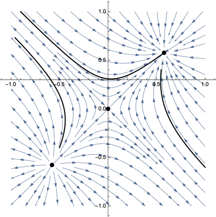
Figure 1: Phase portrait in the plane $H_{a}-H_{b}$ for the quadratic $f\left(T\right)=T+f_{0}T^{2}$ lagrangian, with $f_{0}=\frac{1}{12}$. Solid lines describe real solutions of the field equations.

V Discussion

The main subject of this study was to prove the existence, and study the stability, of the Kasner vacuum solution of Bianchi type I for the modified $f\left(T\right)$ teleparallel gravity. Vacuum solutions have not been studied extensively in  $f\left(T\right)$ gravity, and it was only recently found that there exists an anisotropic vacuum Bianchi I exact solution ftSing in this gravitational context.

In particular, we found conditions under which a nonlinear $f\left(T\right)$ gravity provides solutions of TEGR and discussed their features. Those conditions applied in two functional forms for $f\left(T\right)$ gravity where there was a special interest in the dark energy section; specifically, for the power-law $f(T)$ model (25) and the exponential $f(T)$ model (26). The assumption that the Kasner universe solves the field equations was found to place a number of constraints on the free parameters of the $f\left(T\right)$ models in question. The power-law model (25) admits the Kasner solution only if the power in $T^{n}$ satisfies $n\geq 2$; while for the exponential model (26), it was found that the exponential model presented in ref.Lin2010 does not yield a Kasner universe solution.

We performed a perturbation of the Kasner solution and study the linearized field equations in a number of cases. We solved the perturbation equations directly and analysed for the critical points. We found that the perturbation equations admit a logarithmic singularity, which correlates with the fact that the fixed-point analysis shows the Kasner solution to be a saddle point. Therefore, the Kasner universe turns out to be unstable in $f\left(T\right)$ gravity.

Additionally, in order to better understand the evolution of the field equations, a fixed-point analysis was performed which resulted in the power-law model providing a future attractor which was an isotropic de Sitter universe. Therefore, we can claim that in $f\left(T\right)$ gravity, small fluctuations in the (anisotropic) Kasner universe can lead evolve towards an accelerating de Sitter universe. This is demonstrated in the phase portrait shown in Fig. 2, where the anisotropic Hubble parameters

$$\Delta H_{a}=\frac{\left(H_{a}-H_{V}\right)^{2}}{\left(H_{V}\right)^{2}},~{}\Delta H_{b}=\frac{\left(H_{b}-H_{V}\right)^{2}}{\left(H_{V}\right)^{2}}~{},~{}\Delta H_{c}=\frac{\left(H_{c}-H_{V}\right)^{2}}{\left(H_{V}\right)^{2}},$$ (57)

and

$$\Delta H_{tot}=\Delta H_{a}+\Delta H_{b}+\Delta H_{c},$$ (58)

are presented, where $H_{V}$ is the Hubble parameter for the average volume, $H_{V}=\frac{\dot{V}}{V}$, in which the volume factor is $V\left(t\right)\equiv a\left(t\right)b\left(t\right)c\left(t\right)$.

Figure 2: Numerical simulation of the anisotropic Hubble parameters$~{}\Delta H$ for the power-law model, plotted against time (25). Figures are for $n=2\,\$(left) and $n=3~{}$(right) for initial conditions close to the Kasner solution. We observe that the de Sitter Universe is a late-time attractor.

The numerical simulation shown in Fig.(2) is for the power-law model (25) for the cases of $n=2$, $3,$ with initial conditions close to that of Kasner universe. We observe that the anisotropic Hubble parameters ultimately vanish to high accuracy which means that the spacetime evolves to a de Sitter phase, again further adding to the status of the Kasner universe within the $f(T)$ context.

For completeness, let us consider now the $f\left(T\right)=T^{n}$ theory for $n\geq 2$. Now, $f_{T}\left(T\right)_{|T\rightarrow 0}=0$, where the scale factors (23) solve the field equations if and only if

$$p_{1}p_{2}+p_{1}p_{3}+p_{2}p_{3}=0.$$ (59)

As before we perform a linear perturbation on the power-law solution (23), where we see that the perturbations depend on the power $n$ of the theory. In particular, for $n>2$, in which $f_{T}\left(T\right)_{|T\rightarrow 0}$ and $f_{TT}\left(T\right)_{|T\rightarrow 0}=0$, we find that the linear perturbations of the field equations are satisfied identically (unlike in the $n=2$ case), with $f_{TT}\left(T\right)_{|T\rightarrow 0}=2,~{}$where the following differential equation follows:

$$0 = \left(p_{1}+p_{2}\right)t\left(\left(p_{1}+p_{2}\right)\dot{h}_{c}+p_{2}\dot{h}_{a}+p_{1}\dot{h}_{b}\right)+$$ (60)

$$+\left(p_{1}+p_{2}\right)\left(p_{1}\left(p_{1}-3\right)+p_{2}\left(p_{2}-3\right)+p_{1}p_{2}\right)h_{c}+$$

$$+\left(\left(p_{1}\right)^{2}+p_{1}\left(p_{2}-3\right)+p_{2}\left(p_{2}-3\right)\right)\left(p_{2}h_{a}+p_{1}h_{b}\right)$$

where $\mathbf{h}\left(t\right)$ are the perturbations of the Hubble functions for the three different directions; that is, we have considered the perturbation $\mathbf{H}\left(t\right)=\mathbf{H}_{0}\left(t\right)\left(1+\varepsilon\mathbf{h}\left(t\right)\right),$ in which $\mathbf{H}_{0}\left(t\right)$ denotes the zero-order solution (23).  For $n>2,$ we search for higher-order corrections, and we find that for the $n^{th}$ correction equation that (60) follows.

From the above, we conclude that for the $f\left(T\right)=T^{n},$ with $n\geq 2,$ the stability of the Kasner Universe (24) and of the Kasner-like solution (59) depend on the nature of the perturbations. For instance, if we assume that $h_{a}$ and $h_{b}$ decay with a power of $t^{-1}$, then $h_{c}\left(t\right)$ is given by the expression

$$h_{c}\left(t\right)\simeq t^{A\left(p_{1},p_{2}\right)}+h_{c}^{0}t^{B\left(p_{1,}p_{2}\right)},$$ (61)

from which it follows that $A\left(p_{1},p_{2}\right)$ and $B\left(p_{1},p_{2}\right)$ are negative constants iff $p_{1},p_{2}$ have values from the grey grid in Fig. 3

Figure 3: Points on the plane $\left(p_{1},p_{2}\right)$ for which the perturbation (61) decays so that the Kasner-like solution (59) is stable when $h_{a}\left(t\right),~{}h_{b}\left(t\right)$ decays as a power of $t^{-1}$.

By comparing our results for the $f\left(T\right)$ theory of gravity with those for the $f\left(R\right)$ theories of gravity barcl we see that, while there are some similarities in the existence of Kasner-like solutions, there are differences between these two families of theories with regard to the stability of the Kasner-like solution. Such differences have been observed before in the case of an isotropic universe, (see the discussion in ftSing ), and those differences are expected between these two different classes of theories because of the different number of degrees of freedom that they each support.

- (1) A. G. Riess et al., Astron. J. 116, 1009 (1998).
- (2) S. Perlmutter et al., Astrophys. J. 517, 565 (1999).
- (3) T. Clifton, P.G. Ferreira, A. Padilla and C. Skordis, Phys. Rept. 513, 1 (2012)
- (4) S. Weinberg, Gravitation and Cosmology: Principles and Applications of the General Theory of Relativity (Wiley, New York, 1972).
- (5) J. Martin, Comptes Rendus Physique 13, 566 (2012)
- (6) J.D. Barrow and A.C. Ottewill, J. Phys. A. 16, 2757 (1983)
- (7) A. Einstein 1928, Sitz. Preuss. Akad. Wiss. p. 217; ibid p. 224
- (8) M. Tsamparlis, Phys. Lett. A 75, 27 (1979)
- (9) G.R. Bengochea and R. Ferraro, Phys. Rev. D 79, 124019 (2009)
- (10) E.V. Linder, Phys. Rev. D 81, 127301 (2010)
- (11) M. Krššák and E.N. Saridakis, Class. Quantum Grav. 33, 115009 (2016)
- (12) B. Li, T.P. Sotiriou and J.D. Barrow, Phys. Rev. D 83, 064035 (2011)
- (13) B. Li, T.P. Sotiriou and J.D. Barrow, Phys. Rev. D 83, 104030 (2011)
- (14) E. Kasner, Am. J. Math. 43, 217 (1921)
- (15) J. Demaret, M. Henneaux, and P. Spindel, Phys. Lett. B 164, 27 (1985)
- (16) N. Cornish and J. Levin, Phys. Rev. D 55, 7489 (1997)
- (17) A.A. Coley, Dynamical Systems and Cosmology, (Springer Science and Business Media, Dordrecht, 2003)
- (18) K. Adhav, A. Nimkar, R. Holey, Int. J. Theor. Phys. 46, 2396 (2007)
- (19) S.M.M. Rasouli, M. Farhoudi and H.R. Sepangi, Class. Quantum Grav. 28, 155004 (2011)
- (20) X.O. Camanho, N. Dadhich and A. Molina, Class. Quantum Grav. 32, 175016 (2015)
- (21) P. Halpern, Phys. Rev. D 63, 024009 (2001)
- (22) M.V. Battisti and G. Montani, Phys. Lett. B 681, 179 (2009)
- (23) K. Andrew, B. Golen and C.A. Middleton, Gen. Relativ. Gravit. 39, 2061 (2007)
- (24) S.A. Pavluchenko, Phys. Rev. D 94, 024046 (2016)
- (25) J.D. Barrow and T. Clifton, Class Quantum Grav. 23, L1 (2006)
- (26) T. Clifton and J.D. Barrow, Class Quantum Grav. 23, 2951 (2006)
- (27) A. Toporensky and D. Müller, Gen. Relativ. Gravit. 49, 8 (2017)
- (28) J.D. Barrow and J. Middleton, Phys. Rev. D 75, 123515 (2007)
- (29) Y.B Zeldovich and A.A. Starobinsky, Sov. Phys. JETP 34, 1159 (1972)
- (30) J.D. Barrow and M.S. Turner, Nature 291, 469 (1981)
- (31) J.D. Barrow, Nucl. Phys. B 208, 501 (1982)
- (32) J.D. Barrow and S. Hervik, Phys. Rev. D 81, 023513, (2010)
- (33) J.D. Barrow, P. G. Ferreira and J. Silk, Phys. Rev. Lett. 78, 3610 (1997)
- (34) J.D. Barrow, Phys. Rev. D 55, 7451 (1997)
- (35) S.W. Hawking and R.J. Tayler, Nature 209, 1278 (1966)
- (36) J.D. Barrow, Mon. Not. Roy. astr. Soc. 175, 359 (1976)
- (37) J.D. Barrow, R. Juszkiewicz and D.N. Sonoda, Mon. Not. Roy. astron. Soc. 213, 917 (1985)
- (38) D. Saadeh, S.M. Feeney, A. Pontzen, H.V. Peiris and J.D. McEwen, Phys. Rev. Lett. 117, 131302 (2016)
- (39) J. Middleton, Class. Quantum Grav. 27, 225013 (2010)
- (40) M.E. Rodrigues and M.J. Houndjo, D. Saez-Gomez and F. Rahaman, Phys. Rev. D 86, 104056 (2012)
- (41) G.G.L. Nashed, Eur. Phys. J. Plus, 129, 188 (2014)
- (42) A. Paliathanasis, J.D. Barrow and P.G.L. Leach, Phys. Rev. D 94, 023525 (2016)
- (43) J.W. Maluf, Annalen der Physik 525, 339 (2013)
- (44) R. Aldrovandi, J.G. Pereira and K.H. Vu, Braz. J. Phys. 34, 1374 (2004)
- (45) S.G. Turyshev, Ann. Rev. Nucl. Part. Sci. 58, 207 (2008)
- (46) B.P. Abbott et al. (LIGO Scientific and Virgo Collaborations), Phys. Rev. Lett. 116, 221101 (2016)
- (47) K. Bamba, C.Q. Geng, C.C. Lee and L.W. Luo, JCAP 1101, 021 (2011)
- (48) L. Iorio, N. Radicella and M.L. Ruggiero, JCAP 2015, 08 (2015)
- (49) S. Basilakos, Phys. Rev. D 93, 083007 (2016)
- (50) G. Farrugia, J. L. Said and M. L. Ruggiero, Phys. Rev. D 93,104034 (2016)
- (51) R. Ferraro and F. Fiorini, Phys. Rev. D 84, 083518 (2011)