X-Shooter observations of low-mass stars in the
$\eta$ Chamaeleontis association

The nearby $\eta$ Chamaeleontis association is a collection of 4–10 Myr old stars with a disk fraction of 35–45%. In this study, the broad wavelength coverage of VLT/X-Shooter is used to measure the stellar and mass accretion properties of 15 low mass stars in the $\eta$ Chamaeleontis association. For each star, the observed spectrum is fitted with a non-accreting stellar template and an accretion spectrum obtained from assuming a plane-parallel hydrogen slab. Five of the eight stars with an IR disk excess show excess UV emission, indicating ongoing accretion. The accretion rates measured here are similar to those obtained from previous measurements of excess UV emission, but tend to be higher than past measurements from H$\alpha$ modeling. The mass accretion rates are consistent with those of other young star forming regions.

1 Introduction

The evolution of protoplanetary disks affects planet formation and migration. Statistical studies of both excess infrared and H$\alpha$ emission demonstrate that the majority of disks dissipate within 2–3 Myrs after the collapse of the parent molecular cloud (e.g., Haisch et al., 2001; Fedele et al., 2010). This timescale sets a limit on the time available to build up the atmospheres of gas giant planets. The evolution and dissipation of disks differs from system to system – a fraction of stars retain their gas and dust disks for 5–10 Myrs.

One such cluster, the $\eta$ Chamaeleontis association (Mamajek et al., 1999b), is located at a distance of $d=94$ pc (van Leeuwen 2007; see discussion in Murphy et al. 2010) with an age of 4$-$10 Myr (e.g., Lawson et al., 2001; Lawson & Feigelson, 2001; Luhman & Steeghs, 2004; Herczeg & Hillenbrand, 2015). The total disk fraction of the association ranges between 35$-$45% if including stars of all masses. Of the 15 canonical low-mass members, 8 retain dust disks as identified from excess IR emission (Megeath et al., 2005; Sicilia-Aguilar et al., 2009), thereby offering a unique opportunity to study disk and stellar properties at stages when giant planet formation should be coming to an end.

In the viscous accretion model of disk evolution (e.g. Hartmann et al., 1998), the accretion rate is expected to decrease with age. The accretion properties of old disks, including those in the $\eta$ Chamaeleontis association, are therefore important to compare to the accretion properties of younger systems. However, these measurements may be complicated because emission from young stars include photospheric and accretion components and are affected by extinction, all of which may vary with time (e.g., Bertout et al., 1988; Basri & Bertout, 1989; Gullbring et al., 1998; Sicilia-Aguilar et al., 2010). Recent improvements in evaluating photospheric and accretion properties of young stars have been driven by simultaneous fits of spectral type, extinction, and accretion luminosity to broadband optical spectra, using young stars as templates (e.g., Manara et al., 2013a, 2016, 2017; Herczeg & Hillenbrand, 2014).

In this paper, we analyze flux-calibrated X-Shooter optical spectra of 15 low-mass members of the $\eta$ Cha cluster to measure accretion and photospheric properties of stars in the association. The paper is structured as follows: After describing the observational setup in Section 2, in Section 3 we determine the stellar parameters and investigate each star for extinction and continuum excess; in Section 4, we investigate each sample member for accretion and infer the accretion luminosity of the accreting PMSs; in Section 5 we present hydrogen emission lines and the derived mass accretion rates. In Section 6 we discuss the results and summarize the study in Section 7.

Table 1: Observation log of VLT/X-Shooter observations in the $\eta$ Cha association

Object	RA(J2000)	DEC(J2000)	Obs. date	Mode	Exp. (UVB)	Exp. (VIS)	Exp. (NIR)
			[UTC]		[s]	[s]	[s]
J0836.2-7908 (J0836)	8 36 10.27	$-$79 08 17.65	2010-01-20	NOD	800	790	780
RECX 1	8 36 55.77	$-$78 56 45.71	2010-01-18	NOD	48	20	40
J0838.9-7916 (J0838)	8 38 50.65	$-$79 16 13.66	2010-01-18	NOD	200	180	200
J0841.5-7853 (J0841)	8 41 29.24	$-$78 53 03.45	2010-01-19	NOD	360	388	388
RECX 3	8 41 36.46	$-$79 03 27.97	2010-01-20	NOD	220	240	240
RECX 4	8 42 23.07	$-$79 04 00.60	2010-01-18	NOD	100	90	80
RECX 5	8 42 26.37	$-$78 57 44.48	2010-01-19	NOD	120	96	120
RECX 6	8 42 38.71	$-$78 54 41.97	2010-01-20	NOD	170	180	180
RECX 7	8 43 07.19	$-$79 04 50.84	2010-01-20	STARE	55	60	60
J0843.3-7915 (J0843)	8 43 17.24	$-$79 05 16.74	2010-01-18	NOD	100	90	100
J0844.2-7833 (J0844)	8 44 08.61	$-$78 33 45.25	2010-01-18	NOD	460	480	460
RECX 9	8 44 15.65	$-$78 59 05.43	2010-01-19	NOD	240	60	240
RECX 10	8 44 30.81	$-$78 46 29.02	2010-01-19	NOD	100	90	100
RECX 11	8 47 01.25	$-$78 59 34.02	2010-01-18	NOD	50	30	40
RECX 12	8 47 55.72	$-$78 54 52.74	2010-01-19	NOD	100	120	120

2 Observations and data reduction

As part of a survey on T Tauri stars in the $\eta$ Cha association and Chamaeleon I and II (Manara et al. 2016; Program ID 084.C-1095, PI: Herczeg), a sub-sample of $\eta$ Cha cluster members have been observed with the ESO/VLT X-Shooter echelle spectrograph over three nights in January 2010 (Table 3). The X-Shooter sample consists of 15 low-mass stars among the cluster members found by, e.g., Luhman & Steeghs (2004). Four new probable cluster members and three potential members were identified by Murphy et al. (2010) in the outskirts of the cluster, after the observations presented here had been conducted, and are therefore not included in our sample.

The X-Shooter spectrograph covers a broad wavelength range, from 300 nm to 2500 nm using three different arms (UVB: $\lambda\lambda$ 300–550 ${\rm nm}$, VIS: $\lambda\lambda$ 550–1000 ${\rm nm}$, NIR: $\lambda\lambda$ 1000–2500 ${\rm nm}$, (Vernet et al., 2011)). To optimize the flux calibration, we combined short (from 3–65 seconds) broad-slit ($1\aas@@fstack{\prime\prime}5-5\aas@@fstack{\prime\prime}0$) and deep (from 20–800 seconds) narrow-slit ($0\aas@@fstack{\prime\prime}4-1\aas@@fstack{\prime\prime}0$) observations. The observation log is given in Table 3. In this paper we present the optical spectra extracted from the UVB and VIS arms.

Data reduction, carried out with the X-Shooter pipeline XSH 1.2.0 (Modigliani et al., 2010), consisted of bias and flat-field corrections, combination of single frames obtained in the “NODDING” mode, wavelength calibration, rectifying each order, and then merging the orders. The extraction of the spectra and the sky removal were performed with the IRAF  task apall.

The response function was measured using the spectro-photometric standard star GD 71 (Hamuy et al., 1994; Vernet et al., 2009) observed at the beginning of each night. Since the comparison of the response functions from the individual nights only yielded small differences, all UVB-arm observations were calibrated with the response function derived from the first night and all VIS-arm observations with an average response function of all three nights.

In order to account for wavelength-dependent slit losses, narrow-slit observations are scaled to the broad-slit observations with low order polynomials fitted to spectral regions with high signal to noise. The stability and accuracy of the flux calibration is estimated by comparing observations of telluric standards across all nights. Figure 1 shows the comparison of multi-epoch X-Shooter spectra of three standards stars with optical photometry: $B_{T},V_{T}$ band photometry from Tycho-2 catalogue and $R$ band from the NOMAD catalogue. In general, the observed spectra agree well with the photometry, with fluxes at $B$, $V$, and $R$-band wavelengths located within the error bars of the photometry and an overall scatter in all standards of $\sim$$4\%$. Based on this comparison the flux calibration accuracy is $\sim$$4\%$.

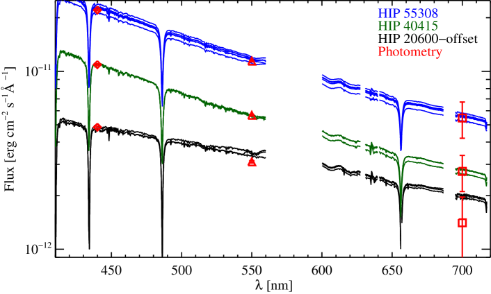
Figure 1: Comparison of telluric standards HIP 55308 (blue), HIP 40415 (green) and HIP 20600 (black), observed in different epochs (multiple instances of one color), with literature photometry (red) in the $B$-band (diamonds), $V$-band (triangles) and $R$-band (squares). The spectra of HIP 20600 and the corresponding photometry are displayed with a constant offset of $1\times 10^{-12}\,{\rm erg\,s^{-1}\,cm^{-2}\,\AA^{-1}}$.

3 Stellar parameters

Measurements of stellar parameters for low-mass pre-main sequence stars may be contaminated by the accretion continuum, which if not considered can lead to degeneracies between spectral type, extinction, and accretion measurements. These degeneracies are minimized when measuring stellar parameters from flux-calibrated optical spectra that cover a wide wavelength range (e.g., Manara et al., 2013a; Herczeg & Hillenbrand, 2014; Alcalá et al., 2014). In this section we first estimate spectral type (SpT) and veiling following Herczeg & Hillenbrand (2014). Based on this initial estimate, we then perform a grid comparison of the program stars with stellar templates of different SpT, and different veiling and extinction values. Finally, the physical stellar properties (effective temperature ($T_{\rm eff}$), luminosity ($L_{*}$), radius ($R_{*}$) and mass ($M_{*}$)) are inferred using tabulated conversions, and from comparison with evolutionary tracks on the Hertzsprung-Russell diagram.

3.1 Spectral types

Our initial spectral types are calculated from atomic absorption and molecular bands, quantified in the spectral indices R5150, TiO6800, TiO7140 and TiO8465 that were developed for young stars (Herczeg & Hillenbrand, 2014). The indices TiO6800, TiO7140 and TiO8465 compare integrated flux within the absorption and the continuum band. For R5150, a linear fit over low and high wavelength continuum regions is used to estimate the continuum on the band. In two cases, J0843 and J0844, these indices are corrected for veiling (see Sect. 3.2). These spectral types agree with those that would have been measured from the TiO7140 index of Jeffries et al. (2007).

Table 7 lists the spectral type obtained from each index, which combine to form an initial estimate of spectral type. The final spectral types are adopted in Sect. 3.3 by comparing the spectra to a grid of spectra of non-accreting young stars.

Table 2: Spectral types derived from spectral indices and adopted values after comparison to non-accreting PMS

Object	R5150	TiO6800	TiO7140	TiO8465	JTiO7140	Adopted
	(K0-M0)	(K5-M0.5)	(M0-M4.5)	(M4-M8)	(K5-M7)
J0836	-	-	-	M5.70	M6.4	M5.5
RECX 1	K5.7	K5.4	-	-	K6.4	K6.0
J0838	-	-	-	M5.3	M5.9	M5.5
J0841	-	-	-	M5.1	M5.6	M5.0
RECX 3	-	-	M3.60	-	M3.7	M3.5
RECX 4	-	-	M1.7	-	M1.3	M1.5
RECX 5	-	-	M4.5	M4.2	M4.5	M4.5
RECX 6	-	-	M3.1	-	M3.2	M3.0
RECX 7	K5.6	K6.0	-	-	K6.9	K6.0
J0843	-	-	M3.6	-	M3.7	M4.0
J0844	-	-	-	M6.1	M5.5	M6.0
RECX 9	-	-	-	M4.7	M5.2	M4.5
RECX 10	-	K8.4	M0.7	-	M0.2	M0.0
RECX 11	K5.7	K5.2	-	-	K6.0	K6.0
RECX 12	-	-	M3.0	-	M3.1	M3.0

3.2 Veiling estimates

Veiling describes the change of the depth of photospheric absorption lines due to excess continuum emission (e.g Basri & Batalha, 1990). Veiling at blue wavelengths is measured in the gravity-sensitive Ca i $\lambda 422.7$ nm absorption line, following the approach of Herczeg & Hillenbrand (2014) but adapted to higher spectral resolution using the non-accreting photospheric templates from Manara et al. (2013b). For templates, the relationship between spectral type and equivalent width (Fig. 2) is described by

$$\mathrm{EW}_{\mathrm{CaI}\leavevmode\nobreak\ \lambda\mathrm{422.7nm}}=-31.7+0.676\times\mathrm{SpT},$$ (1)

where SpT is spectral type and a spectral type of M0 is equivalent to ${\rm SpT}=58$. Fig. 2 shows that most $\eta$-Cha-cluster objects have equivalent widths consistent with those expected from the templates. These objects are assumed to have negligible veiling.

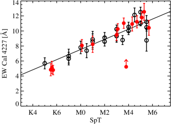
Figure 2: Equivalent width of Ca i $\lambda 422.7$ nm line vs. spectral type. Red filled circles denote observations presented in this work, black empty circles are from template stars (Manara et al., 2013b). Due to strong emission lines inside the absorption feature, we determine a lower limit for J0843 (red arrow). The black line denotes the relation between the equivalent width and spectral type of a non-accreting stars (Eq. 1).

Two objects, J0843 and J0844, show significant veiling. The Ca i $\lambda 422.7$ nm absorption feature in J0843 is detected but blended with emission lines. Assuming that the absorption profile is Gaussian with similar width as the template spectra, the lower limit on the Ca i equivalent width is estimated to be at 5.2 Å (Fig. 3), implying a veiling of $r_{\mathrm{4}22.7{\,}{\rm nm}}\lesssim 1$ (Eq. 1). The absorption feature is not detected in J0844 (Fig. 3), indicating that the veiling is high.

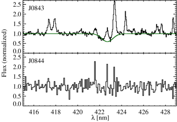
Figure 3: Continuum-normalized spectrum around the Ca i $\lambda 422.7$ nm absorption line (black) for the veiled stars J0843 (top) and J0844 (bottom). The absorption line from J0843 is contaminated by emission in the same transition. The equivalent width, and subsequently the veiling, are measured by fitting a Gaussian profile (green) to the spectrum, avoiding regions with emission. The absorption line from J0844 is not detected.

3.3 Grid comparison with PMS stellar templates

In order to verify the spectral type and veiling, we compare each spectrum to a set of pre-main sequence, non-accreting stellar templates obtained from the X-Shooter library of young stars (Manara et al., 2013b). We model veiling and extinction simultaneously by adding constant accretion continuum flux to the template (Herczeg & Hillenbrand, 2014), and by convolving each model with the extinction curve of Cardelli et al. (1989), with a total-to-selective extinction of $R_{V}=3.1$. The best-fit parameters are initially determined from spectral fits and are then tweaked manually to obtain the best visual representation of the spectrum.

All objects without veiling in the Ca i $\lambda 422.7$ nm absorption feature (see Sect. 3.2) are best modeled without adding excess flux longward of 400 nm. All sources, including those with ongoing accretion, are also well fit with no reddening, consistent with previous studies (e.g., Luhman & Steeghs, 2004).

An iterative approach is used for the two objects with strong veiling in the Ca i $\lambda 422.7$ line, J0843 and J0844. For the final models, the extinction is fixed at $A_{V}=0$ mag. The templates are fixed to the pre-main sequence stars TWA 9B (TW Hya association, SpT = M3) and SO925 ($\sigma$ Ori region, SpT = M5.5; Manara et al. 2013b). The best-fit value for the veiling at 751 nm is $r_{751}=0.05$ in both objects. The veiling translates to excess fluxes of $f_{\rm excess}=9.1\times 10^{-16}\,{\rm erg\,s^{-1}\,cm^{-2}\,\AA^{-1}}$ for J0843 and $f_{\rm excess}=6.9\times 10^{-17}\,{\rm erg\,s^{-1}\,cm^{-2}\,\AA^{-1}}$ for J0844. After accounting for this veiling, the spectral type from spectral indices changes to M4.0 for J0843 and stays at M6.0 for J0844.

The final spectral types are listed to a precision of one subclass for stars earlier than M0 and to 0.5 subclasses for stars later than M0, adopting the spacing of the sample of non-accreting template stars (see also Manara et al., 2013b).

3.4 Effective temperature, luminosity and stellar radius

Table 3: Stellar parameters - Literature comparison

Object	SpT	SpT	SpT	$T_{\rm eff}$ [K]	$T_{\rm eff}$ [K]	$L_{\ast}$ [$L_{\odot}$]	$L_{\ast}$ [$L_{\odot}$]	$L_{\ast}$ [$L_{\odot}$]
	(Luhman)	(Lyo)		(Luhman)		(2MASS-J)	(Lyo)
J0836	M5.5	M5.3	M5.5	3058	2920	0.020	0.020	0.0190
RECX1	K6	K7.0	K6.0	4205	4115	0.880	1.000	0.9800
J0838	M5.25	M5.0	M5.5	3091	2920	0.034	0.035	0.0340
J0841	M4.75	M4.7	M5.0	3161	2980	0.021	0.023	0.0210
RECX3	M3.25	M3.0	M3.5	3379	3300	0.089	0.097	0.1000
RECX4	M1.75	M1.3	M1.5	3596	3640	0.210	0.240	0.2000
RECX5	M4	M3.8	M4.5	3270	3085	0.056	0.062	0.0670
RECX6	M3	M3.0	M3.0	3415	3410	0.100	0.110	0.1000
RECX7	K6	K6.9	K6.0	4205	4115	0.690	0.790	0.7000
J0843	M3.25	M3.4	M4.0	3379	3190	0.074	0.083	0.0730
J0844	M5.75	M5.5	M6.0	3024	2860	0.011	0.010	0.0078
RECX9	M4.5	M4.4	M4.5	3198	3085	0.090	0.096	0.0950
RECX10	M1	M0.3	M0.0	3705	3900	0.210	0.230	0.2100
RECX11	K5.5	K6.5	K6.0	4278	4115	0.530	0.590	0.4600
RECX12	M3.25	M3.2	M3.0	3379	3410	0.240	0.250	0.2300

(1) Luhman & Steeghs (2004); (2) Lyo et al. (2004); (3) Cutri & et al. (2012); Herczeg & Hillenbrand (2015).

We derive effective temperatures from spectral types using the conversion table proposed by Herczeg & Hillenbrand (2014) (see also Pecaut & Mamajek, 2013), as estimated by comparing optical spectra of young templates to the recent BT-Settl models of synthetic spectra (Allard et al., 2012).

Stellar luminosities are obtained from the continuum flux at 751 nm and using the bolometric flux conversion table from Herczeg & Hillenbrand (2014). For J0843 and J0844, the estimated flux in the accretion continuum at 751 nm (see Sect. 3.3) is subtracted before calculating $L_{*}$. The stellar radius is then calculated from the Stefan Boltzmann law, $L_{*}=4\pi R_{*}^{2}\sigma T_{\mathrm{eff}}^{4}$. The results are listed in Table 4.

In Table 3 we compare the derived stellar parameters with previous classifications of the $\eta$ Cha association (Luhman & Steeghs, 2004; Lyo et al., 2004). Spectral types agree well within uncertainties. Consistent with the errors of the classification, there is a small trend of spectral types in this work being slightly earlier for early M stars and later for late M stars. The effective temperatures are systematically colder for cold objects, which is due to the different SpT-$T_{\mathrm{eff}}$ conversions used in this work. Use of the Pecaut & Mamajek (2013) SpT-$T_{\mathrm{eff}}$ scale would have led to even lower temperatures for these stars.

Measured stellar luminosities agree well within errors (see Table 3) to both previous measurements (Lyo et al., 2004) and to luminosities inferred from $J$-Band (Cutri & et al. 2012; using bolometric corrections from either Pecaut & Mamajek 2013 or Herczeg & Hillenbrand 2015).

3.5 The Hertzsprung-Russell diagram

We use stellar isochrones from Baraffe et al. (2015) to infer stellar ages and masses. The isochrones are first mapped to a finer grid in $T_{\rm eff}$. For a given grid-$T_{\rm eff}$ value, the isochrones are interpolated onto a finer age grid. The adopted stellar mass is given by the closest grid value in $T_{\rm eff}$ and $L_{*}$.

Fig. 4 shows the sample overplotted with evolutionary tracks from Baraffe et al. (2015). A large fraction of the sample (2/3) lies between the 1-Myr and 5-Myr isochrones, approximately following the trend of the isochrones. The known binaries are located above the single stars. The median age of single stars hotter than 3300 K is 5 Myr. This agrees well with some of the previous results (Luhman & Steeghs, 2004; Herczeg & Hillenbrand, 2015) and place the $\eta$ Cha cluster at a significantly younger age than others (e.g., 11$\pm$3 Myr, Bell et al., 2015). As a general caveat, masses and ages inferred from Hertzsprung-Russell diagrams may be misleading for low-mass stars when spectra are fit with single-temperature photospheres (e.g., Gully-Santiago et al., 2017).

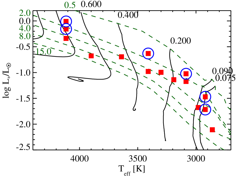
Figure 4: Hertzsprung-Russell diagram of the $\eta$ Cha association. Evolutionary tracks (mass in $M_{\odot}$) are shown as black solid lines and isochrones (age in Myr) as green dashed lines (both Baraffe et al. 2015). $\eta$ Cha cluster stars are drawn as red squares. Binary stars are encircled in blue (as in table 1 of Sicilia-Aguilar et al., 2009).

Table 4: Derived stellar parameters in the $\eta$ Cha association

Object	$T_{\rm eff}$	$f_{751}$	$L_{\ast}$	$R_{\ast}$	$M_{\ast}$	Infrared Class1
	[K]	$[1{\rm x}10^{-13}\,{\rm erg\,s^{-1}\,cm^{-2}\,\AA^{-1}}]$	[$L_{\odot}$]	[$R_{\odot}$]	[$M_{\odot}$]
J0836	2920	0.038	0.019	0.54	0.069	Class III
RECX1	4115	3.100	0.980	1.90	0.750	Class III
J0838	2920	0.066	0.034	0.72	0.075	Class III
J0841	2980	0.043	0.021	0.54	0.086	TO/flat
RECX3	3300	0.280	0.100	0.98	0.250	TO
RECX4	3640	0.620	0.200	1.10	0.460	TO
RECX5	3085	0.150	0.067	0.91	0.150	TO
RECX6	3410	0.300	0.100	0.93	0.320	Class III
RECX7	4115	2.200	0.700	1.60	0.780	Class III
J0843	3190	0.180	0.073	0.88	0.200	Class II
J0844	2860	0.014	0.008	0.36	0.052	flat
RECX9	3085	0.220	0.095	1.10	0.150	TO
RECX10	3900	0.670	0.210	1.00	0.690	Class III
RECX11	4115	1.500	0.460	1.30	0.830	Class II
RECX12	3410	0.680	0.230	1.40	0.290	Class III

(1) Infrared disk classifications as in Sicilia-Aguilar et al. (2009).

4 Mass accretion rate

In this section, we measure accretion rates and upper limits of our sample from UVB-arm spectra of X-Shooter. Section 4.1 discusses the Balmer Jump as a diagnostic of excess continuum emission produced by ongoing accretion. The excess flux is quantified by modeling the observed spectrum, as described in Sect. 4.2, and used to derive the mass accretion rate. The model consists of non-accreting PMS spectra as proxies for photospheric emission of young stars and the emission of a plane-parallel slab as proxy for the radiation from regions heated in the accreting process. While the emission from the plane-parallel hydrogen slab is not a physical model (for physical models see, e.g., Calvet & Gullbring, 1998; Ingleby et al., 2013), the accretion spectrum provides a reasonable fit to the continuum emission and a reasonable bolometric correction to account for emission outside of the observed spectral range. Individual objects are discussed in Sect. 4.3.

4.1 The Balmer jump

The presence of excess Balmer-continuum emission produced by accretion is quantified here by measuring Balmer Jump, defined as the flux ratio $f(360{\,}\textrm{nm})/f(400{\,}\textrm{nm})$. The X-Shooter UVB spectra are shown in Figures 6 and 7 along with template, non-accreting, PMS stars (Manara et al., 2013b; Stelzer et al., 2013), with results on the Balmer jump shown in Fig. 5. The dashed line ($f(360{\,}\textrm{ nm})/f(400{\,}\textrm{nm})$ = 0.5) indicates the threshold between accreting and non-accreting sources (Herczeg et al., 2009), consistent with the non-accreting templates of Manara et al. (2013b).

Of the $\eta$ Cha cluster members, seven sources show a Balmer Jump above this threshold. Three sources have strong UV-excess emission (RECX 5 (Balmer Jump $\sim$ 0.8), J0843 (2.1) and J0844 (2.6)), while four have a moderate excess (between 0.5$-$0.6: RECX 11, RECX 12, RECX 9 and J0838). In the case of J0838, the continuum level at 360 nm is enhanced with respect to the template, while at wavelengths below 355 nm the spectrum agrees with the template within the noise (Fig. 6). The enhanced Balmer Jump of this star is therefore not considered as an indicator of accretion. The UV-excess in RECX 12 is attributed to chromospheric activity, as the H$\alpha$ line is narrow and has an equivalent width which is lower than expected for mass accretion (see Sect. 5), and has a UV spectrum consistent with the non-accreting template TWA 15A (Fig. 6). RECX 12 is discussed in more detail in Sect. 5. The UV-excess is clearly visible in the spectra of RECX 9 and RECX 11.

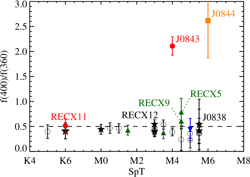
Figure 5: Observed Balmer jump of the $\eta$ Cha cluster members (filled symbols) and non-accreting PMSs from Manara et al. (2013b), which were used as templates in this work (black empty circles). The black dashed line highlights an observed Balmer jump of 0.5. The shape and color of the filled symbols highlight SED classifications from Sicilia-Aguilar et al. (2009): Black stars denote Class III objects, red circles Class II objects, green triangles transitional objects, the blue, inverted triangle the transitional/flat object J0841, and the orange box the flat source J0844.

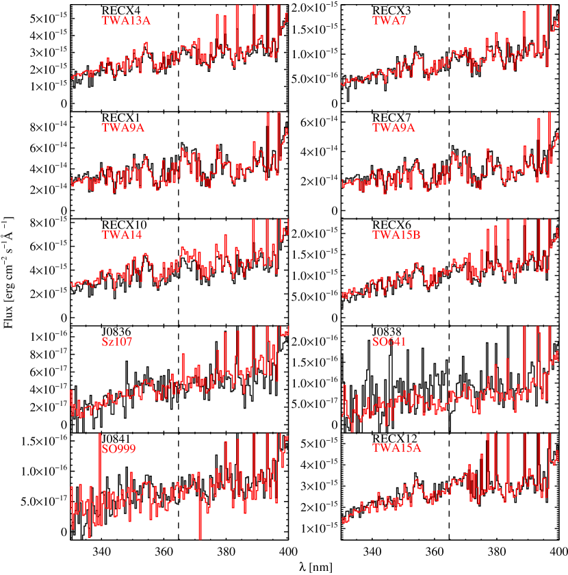
Figure 6: Comparison of the UV spectrum for stars with an observed Balmer jump ratio typical for non-accreting stars (black), with template stars from Manara et al. (2013b) of similar spectral type (red; template names as in Manara et al. 2013b). The spectra are binned to 0.5 nm resolution and the templates are scaled to the target at 450 nm. The dashed vertical line shows the theoretical location of the Balmer jump.

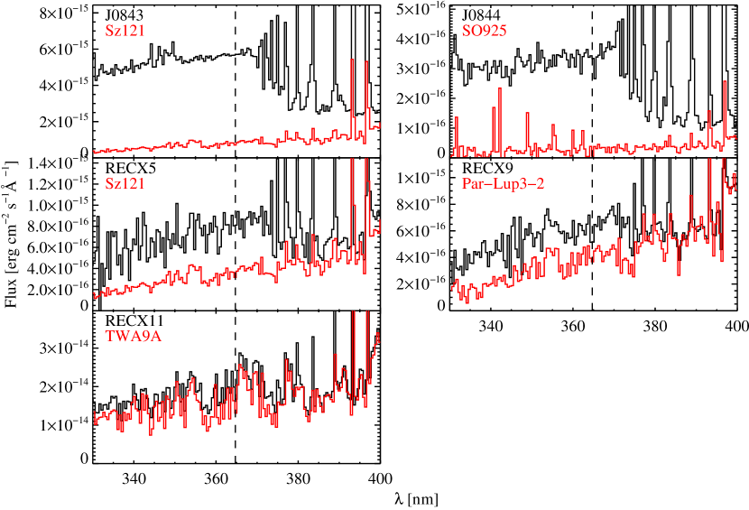
Figure 7: As Fig. 6. J0843, J0844 and RECX 5 and RECX 9 show clear indications of UV-excess. For RECX 11, a slight excess is seen.

4.2 Method of Fitting the UV-excess

The accretion continuum, modeled from a pure-hydrogen isothermal slab, is added to the photospheric template (see Sect. 3.3) to best fit the UV spectrum of the accreting star. The grid of slab models (Valenti et al., 1993) spans a parameter space in density and temperature of the hydrogen gas (Table 5), where the length of the slab is fixed to $l=2\textrm{ x }10^{7}$ cm (Herczeg et al., 2009). The bolometric correction is calculated by summing the accretion continuum luminosity over all wavelengths.

Best-fit parameters are calculated by minimizing a $\chi^{2}$-like function over multiple wavelength bands in the UVB arm of X-Shooter, with wavelengths selected to exclude sharp emission and absorption lines. The $\chi^{2}$-like minimization function is defined as $\chi^{2}_{\mathrm{like}}=\sum_{\mathrm{bands}}\left({\frac{\overline{f_{\mathrm{obs}}}-\overline{f_{\mathrm{model}}}}{\sigma(f_{\mathrm{obs}})}}\right)$, where $\overline{f_{\mathrm{obs}}}$ and $\overline{f_{\mathrm{model}}}$ denote the median of each band in the observed spectrum and model, and $\sigma(f_{\mathrm{obs}})$ gives the standard deviation in each band in the observed spectrum. As also described in Manara et al. (2013a), this does not represent a true $\chi^{2}$ distribution, as the noise in the template spectrum is neglected. The models are visually compared to confirm that the best-fit model matches the observed spectrum. The uncertainties are estimated from the range of UV-excess fluxes spanned by models that yield a similar $\chi^{2}$-like value as the best-fit model and match the spectrum visually (details are described in Sect. 4.3).

Table 5: Parameter ranges of the hydrogen slab model

	Min.	Max.	Step size
$T_{\rm eff}{\rm[K]}$	6000	11000	500
${\rm log(n_{H}[cm^{-3}])}$	12	15	0.01

The measured UV-excess flux is converted to accretion luminosity ($L_{\rm acc}$). The mass accretion rates ($\dot{M}$) are then calculated by

$$L_{\mathrm{acc}}=\frac{GM_{*}\dot{M}}{R_{*}}\cdot\left(1-\frac{R_{*}}{R_{\mathrm{trunc}}}\right),$$ (2)

under the assumption that gas accretes from the disk truncation radius $R_{\mathrm{trunc}}$ in free-fall onto the star, where $R_{\rm trunc}=5\,R_{*}$ is adopted for consistency with pre-existing measurements (see review by Hartmann et al., 2016).

4.3 Description of fits and uncertainties

Figures 16 - 19 show the best-fit model for each object. $L_{\rm acc}$ and $\dot{M}$ are listed in Table 11.

Uncertainties in the accretion rates are introduced by uncertainties in the stellar parameters, the distance, and in the individual fits (see, e.g., Herczeg & Hillenbrand, 2008; Manara et al., 2013a). For our sample, uncertainties in $\dot{M}$ are $\sim$0.3 dex. Weak accretors, such as RECX 11, have uncertainties of $\sim$0.5 dex because the excess is fainter than the photosphere, thereby increasing the uncertainty in bolometric correction.

Upper limits on $\dot{M}$ are difficult to estimate and depend on the ability to distinguish any excess emission from the underlying photospheric spectrum and on an uncertain bolometric correction. In order to estimate upper limits of $\dot{M}$ for non-accreting objects, we perform a similar model fit as described above. The upper limits are compared to the detections in Fig. 8a in terms of the ratio of $L_{\rm acc}/L_{*}$. For K stars, the upper limit of $L_{\rm acc}/L_{*}$ for non-accreting stars is similar to $L_{\rm acc}/L_{*}$ of RECX 11. For M stars, the upper limits are rather uniform at ${\rm log}\,L_{\rm acc}/L_{*}\approx-3.0$ (see also Manara et al., 2013b), with the exception of RECX 12 (${\rm log}\,L_{\rm acc}/L_{*}\approx-2.7$).

Comments on each fit to the spectra of accreting objects are provided below.

J0843 and J0844: Due to the pronounced observed Balmer jump and strong excess in Balmer and Paschen continuum, the slab model parameters and therefore the $L_{\rm acc}$ are well constrained. Models using templates within 0.5 spectral subclasses yield accretion rates that agree within 10% of these values.

RECX 5: The best-fit $\dot{M}$ is calculated using the M4 template Sz 121. Model results using the M3 template TWA 9B and or the M5 template Par-Lup3-2 also reproduce the UVB spectrum of RECX 5, yield accretion rates that differ by 30% from the adopted best-fit.

RECX 9: The best-fit $\dot{M}$ is calculated from the M4.5 template SO797. Model results using templates the M5 templates Par-Lup3-2 and SO641 yield accretion rates that differ by 45%.

RECX 11: $\dot{M}$ of RECX 11 is uncertain by a factor of 2.5 because the UV excess is very small, so the slab model fit is not well constrained.

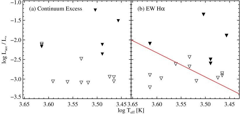
Figure 8: Accretion luminosity (in units of $L_{*}$) vs. $T_{\rm eff}$ for accreting PMS (filled triangles) and upper limits for non-accreting PMS (empty triangles). In panel (a), $L_{\rm acc}$ is derived from continuum excess radiation and in panel (b) from the H$\alpha$ equivalent width. The red line in panel (b) shows the chromospheric contribution from hydrogen emission lines to $L_{\rm acc}$ (Manara et al., 2013b).

5 Line emission

Accretion and related processes produce emission in many detectable lines, a subset of which are analyzed here: The H$\alpha$ and H$\beta$ transitions, the He i${\leavevmode\nobreak\ \lambda 402.6}$, ${{\rm HeI}\leavevmode\nobreak\ \lambda 447.1}$, He i${\leavevmode\nobreak\ \lambda 501.5}$, He i${\leavevmode\nobreak\ \lambda 587.5}$, He i${\leavevmode\nobreak\ \lambda 667.8}$, He i${\leavevmode\nobreak\ \lambda 706.5}$ transitions and blended He i and Fe i lines at 492.2 nm ($\textup{He\,{i}}\textup{Fe\,{i}}\lambda 492.2$, Alcalá et al., 2014), and the [O i]${\leavevmode\nobreak\ \lambda 557.7}$, [O i]${\leavevmode\nobreak\ \lambda 630.0}$, [O i]${\leavevmode\nobreak\ \lambda 636.3}$ forbidden transitions. The flux and equivalent widths of the detected lines is given in Tables 11 and 7 to 10.

Figures 10 and 11 show the H$\alpha$ and H$\beta$ profiles. The detection rate of the two transitions is 100% for H$\alpha$ and $\sim$90% for H$\beta$ throughout the full sample. For J0843, J0844, RECX 5, RECX 9 and RECX 11, the H$\alpha$ line profiles are very broad ($\Delta v>200{\,}$km s^-1) and slightly asymmetric, consistent with accretion. All other sources have narrow, symmetric H$\alpha$ profiles with equivalent widths that are below the mass accretion threshold (White & Basri, 2003), consistent with a chromospheric origin of the line emission.

Transitions of He i are detected in J0844, J0843, RECX 5, RECX 9 and RECX 12 (see Tables 7 to 10). Emission in He i${\leavevmode\nobreak\ \lambda 402.6}$ is weakly detected in J0841. J0836 shows weak emission in the ${{\rm HeI}\leavevmode\nobreak\ \lambda 447.1}$ line. The emission lines for RECX 12 are in all cases weaker than for the accreting stars with detections in He i. To note special line profiles: J0843 shows a broad, blue shifted component at lower flux than the central, narrow peak in the ${{\rm HeI}\leavevmode\nobreak\ \lambda 447.1}$ transition and broad wings in the He i${\leavevmode\nobreak\ \lambda 587.5}$ transition. The He i${\leavevmode\nobreak\ \lambda 501.5}$ line and He i+Fe i blend at $\lambda$ 492.2 are blended with Fe ii emission at slightly higher wavelengths for J0844 and J0843. Fe ii emission has also been found in heavily veiled objects, including some outbursts (e.g., Hessman et al., 1991; Hamann & Persson, 1992; van den Ancker et al., 2004; Fedele et al., 2007; Gahm et al., 2008).

The forbidden [O i]${\leavevmode\nobreak\ \lambda 630.0}$ nm line, a diagnostic of winds (e.g. Hartigan et al., 1995; Simon et al., 2016), is detected from J0843 and J0841, and marginally (¡3$\sigma$) from J0844 and RECX 5. To characterize velocity shifts of the line center, the wavelength solution was re-calibrated at the photospheric Li i $\lambda$670.8 nm line. The [O i]${\leavevmode\nobreak\ \lambda 630.0}$ nm line is blueshifted by 24 km s^-1 for J0843, and not detectably shifted in J0841 (Fig. 9). Additionally, the [O i]${\leavevmode\nobreak\ \lambda 557.7}$ transition is detected from J0843, J0844, RECX 5 and RECX 9, while the [O i]${\leavevmode\nobreak\ \lambda 636.3}$ line is only detected from J0843.

5.1 Notes on individual objects

RECX 12 and J0838 both show a slightly enhanced Balmer jump (Sect. 4.1), along with an equivalent width of the H$\alpha$ line which is consistent with chromospheric emission. We therefore categorize both stars as non-accreting. However, the status of RECX 12 as a non-accretor is uncertain. The H$\alpha$ line has weak line wings that are at levels of smaller than 10% of the peak flux and are asymmetric towards the blue side of the line. The H$\alpha$ 10% width (200$\pm$20 km s^-1) lies at the threshold for accretion (e.g., White & Basri, 2003; Jayawardhana et al., 2003; Natta et al., 2004). Three He i transitions are detected above 3$\sigma$ for RECX 12, but their equivalent widths are lower than any of the clearly accreting objects in the sample and are consistent with strong chromospheric emission. The upper limit on $L_{\rm acc}/L_{*}$, as derived from continuum excess and H$\alpha$ emission, is higher than for non-accreting objects of similar spectral types in the $\eta$ Cha cluster (see Fig. 8a, b). If the emission was interpreted as accretion, then $\dot{M}$ determined from the H$\alpha$ transition and the continuum emission would agree well with each other, while the H$\beta$ and He i emission lines would yield accretion rates that would be 2$-$3 times larger. $\dot{M}$ would therefore be between $1.5-5.0\times 10^{-10}{\,}{\rm M}_{\odot}/{\rm yr}$. However, since some non-accreting young stars share these characteristics (e.g., the PMS TWA15A in Manara et al. 2013b), we interpret this borderline case as more likely a source with strong chromospheric emission.

The detection of [O i] emission in J0841 is unusual, since accretion is not detected in either H$\alpha$ or in the Balmer continuum. However, a disk is detected from excess infrared emission (e.g., Sicilia-Aguilar et al., 2009). The He i $\lambda$402.6 emission in this object is barely detected. Emission of the [O i] line can originate from disk winds, which can be related to the accretion process (e.g., Hartigan et al. 1995; Nisini et al., submitted). Mass accretion rates between $1.2-14\times 10^{-11}{\,}{\rm M}_{\odot}/{\rm yr}$ would be required to produce the luminosity of the [O i] line ($L_{\rm line}$), assuming a $L_{\rm acc}$-$L_{\rm line}$ relation from Natta et al. (2014). The upper limit on $\dot{M}$ from continuum excess emission of $\dot{M}\approx 0.6\times 10^{-11}{\,}{\rm M}_{\odot}/{\rm yr}$ falls slightly below this range. Hence, the origin of [O i] emission in J0841 is unclear.

H$\alpha$ emission of RECX 7 shows a double-peaked profile and has been classified as a spectroscopic binary in the literature (Mamajek et al., 1999a; Lyo et al., 2003). The equivalent width of each component is in agreement with chromospheric emission. The peaks are separated by $\Delta v\approx$ 185 km s^-1. Indication of H$\beta$ emission may be seen in the low velocity component (see lower right-most panel of Fig. 11) but is confused by absorption lines and is not considered significant.

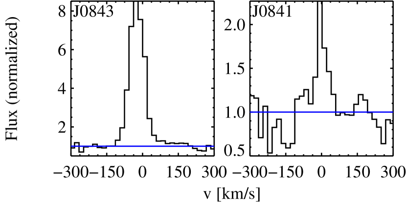
Figure 9: Continuum normalized [O i] ${\leavevmode\nobreak\ \lambda 630.0}$ nm line profiles in J0843 and J0841. In J0843, the line is blue-shifted. The continuum level is indicated by a blue line.

Table 6: Mass accretion properties in the $\eta$ Cha association

Object	$EW_{{\rm H\alpha}\leavevmode\nobreak\ \lambda 656.3}$	$L_{{\rm acc,H}\alpha}$	$\dot{M}_{{\rm H}\alpha}$	$EW_{{\rm H\beta}\leavevmode\nobreak\ \lambda 486.1}$	$L_{{\rm acc,H}\beta}$	$\dot{M}_{{\rm H}\beta}$	$L_{{\rm acc,cont}}$	$\dot{M}_{{\rm cont}}$
	[Å]	[L⊙/yr]	[M⊙/yr]	[Å]	[L⊙/yr]	[M⊙/yr]	[L⊙/yr]	[M⊙/yr]
J0836	$-$13.4$\pm$0.7	¡2.4e-05	¡7.5e-12	$-$11.1$\pm$0.4	¡2.4e-05	¡7.6e-12	¡1.7e-05	¡5.3e-12
RECX1	$-$1.0$\pm$0.1	¡9.0e-04	¡9.4e-11	¡0.2	¡1.7e-04	¡1.8e-11	¡7.2e-03	¡7.5e-10
J0838	$-$12.0$\pm$0.8	¡4.6e-05	¡1.8e-11	$-$10.4$\pm$0.4	¡5.2e-05	¡2.0e-11	¡3.8e-05	¡1.5e-11
J0841	$-$9.5$\pm$0.6	¡2.1e-05	¡5.3e-12	$-$8.3$\pm$0.3	¡2.7e-05	¡6.9e-12	¡2.4e-05	¡6.1e-12
RECX3	$-$2.7$\pm$0.3	¡8.7e-05	¡1.4e-11	$-$1.9$\pm$0.1	¡1.1e-04	¡1.7e-11	¡8.2e-05	¡1.3e-11
RECX4	$-$4.2$\pm$0.3	¡4.9e-04	¡4.9e-11	$-$2.7$\pm$0.2	¡7.3e-04	¡7.2e-11	¡1.7e-04	¡1.7e-11
RECX5	$-$13.5$\pm$0.7	2.1e-04	5.2e-11	$-$14.7$\pm$0.4	4.5e-04	1.1e-10	5.1e-04	1.3e-10
RECX6	$-$5.3$\pm$0.2	¡2.2e-04	¡2.5e-11	$-$4.0$\pm$0.1	¡3.4e-04	¡4.0e-11	¡8.6e-05	¡1.0e-11
RECX7	$-$0.8$\pm$0.1	¡4.3e-04	¡3.6e-11	¡0.2	¡9.5e-05	¡8.1e-12	¡5.6e-03	¡4.7e-10
J0843	$-$94.5$\pm$2.6	3.2e-03	5.8e-10	$-$42.6$\pm$0.7	3.3e-03	5.9e-10	4.2e-03	7.6e-10
J0844	$-$102.2$\pm$5.5	9.8e-05	2.7e-11	$-$82.1$\pm$2.0	2.0e-04	5.5e-11	2.4e-04	6.6e-11
RECX9	$-$12.6$\pm$0.5	2.4e-04	6.8e-11	$-$10.7$\pm$0.3	3.1e-04	9.0e-11	4.1e-04	1.2e-10
RECX10	$-$1.7$\pm$0.2	¡2.2e-04	¡1.3e-11	$-$1.2$\pm$0.2	¡4.2e-04	¡2.5e-11	¡1.8e-04	¡1.1e-11
RECX11	$-$8.3$\pm$0.3	3.9e-03	2.5e-10	$-$2.7$\pm$0.2	5.0e-03	3.2e-10	3.1e-03	2.0e-10
RECX12	$-$8.4$\pm$0.2	¡8.6e-04	¡1.6e-10	$-$8.2$\pm$0.2	¡1.9e-03	¡3.6e-10	¡7.7e-04	¡1.5e-10

5.2 Mass accretion rates from Hydrogen emission lines

Table 11 lists $L_{\rm acc}$ and $\dot{M}$ derived from the line luminosities of H$\alpha$ and H$\beta$ using empirical $L_{\rm acc}$-$L_{\rm line}$ relations (Alcalá et al., 2014). The ratio $L_{\rm acc,H\alpha}/L_{*}$ is shown in Fig. 8b.

For J0843, the accretion rates derived from different tracers agree within 10%. For J0844, RECX 5 and RECX 9, $\dot{M}_{\rm H\alpha}$ is lower by about a factor of two, however $\dot{M}_{\rm H\beta}$ is closer to and within errors of $\dot{M}$ obtained from the continuum excess. A possible reason for this discrepancy could be that the H$\alpha$ line becomes easily optically thick and may be influenced by outflows (e.g., Alcalá et al., 2014). Accretion rates, which are derived from $L_{\rm line,H\alpha}$, agree closely with the accretion rates determined by direct modeling of the H$\alpha$ line profile (Lawson et al., 2004).

The H$\alpha$ equivalent width of RECX 11 is significantly higher than for the other K stars in this sample (RECX 1 and RECX 7) and falls in the range which is typically found for accreting stars at this spectral type (White & Basri, 2003), despite weak continuum emission (see Fig. 8). The H$\alpha$ line of RECX 11 is also affected by red-shifted absorption from the accretion flow (see also Ingleby et al., 2011). $\dot{M}_{\rm H\alpha}$ and $\dot{M}_{\rm H\beta}$ are higher than but within the uncertainties of $\dot{M}$ determined from UV-excess.

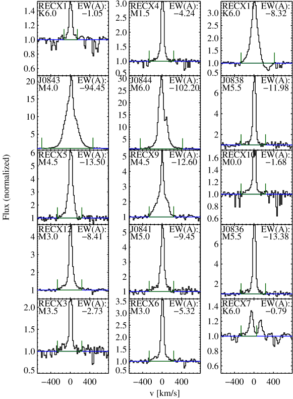
Figure 10: Continuum normalized H$\alpha$ line profiles in the $\eta$ Cha association. Green lines denote the integration boundaries for the determination of line flux and equivalent width. The continuum level is indicated by a blue line. Each panel shows the object’s name, its spectral type and the measured equivalent width (EW).

Figure 11: Line profiles of the H$\beta$ ${\lambda 486.13}$nm transition. Symbols and colors as in Fig. 10.

6 Discussion

6.1 Detectability of mass accretion

H$\alpha$ emission is detected in all sources, generated by either the accretion flow or chromospheric activity. As seen in Fig. 8b, the $L_{\rm acc}/L_{*}$ ratio of accreting stars is higher than the upper limits inferred for non-accreting PMS. The upper limits on $L_{\rm acc,H\alpha}/L_{*}$ are consistent with the threshold for ”accretion noise” inferred by Manara et al. (2013b).

Detection limits for mass accretion rates from UV-excess depend on the spectral type of the star. For M-stars, the detection limits are at $\dot{M}\approx 1\times 10^{-11}{\,}{\rm M}_{\odot}/{\rm yr}$ (Table 11). For the K-stars RECX 7 and RECX 1 (${\rm log}T_{\rm eff}>3.6$), the upper limits of $\dot{M}\approx 4-8\times 10^{-10}{\,}{\rm M}_{\odot}/{\rm yr}$ are higher than $\dot{M}$ of the accretor RECX 11. Unlike for M-stars, these upper limits do not reflect the detection limit but the large uncertainty in fitting the weak UV-excess emission in the warmer K-stars (see Sect. 4.3).

6.2 Variability

The accretion rate has been previously measured on 4 of the 5 accretors in $\eta$ Cha identified here. Our accretion rates obtained from excess Balmer continuum emission are consistent with past measurements using similar approaches but in several cases differ when compared with H$\alpha$-based measurements.

J0843: Our accretion rate is similar to the UV-excess accretion rate $8\times 10^{-10}{\,}{\rm M}_{\odot}/{\rm yr}$ measured by Ingleby et al. (2013) and is 1.25 times lower than the rate of $1\times 10^{-9}{\,}{\rm M}_{\odot}/{\rm yr}$ measured from modeling the H$\alpha$ line by Lawson et al. (2004). All three measurements agree within errors.

RECX 9: Our accretion rate is larger than previous measurements by a factor of three (Lawson et al. 2004; $4\times 10^{-11}{\,}{\rm M}_{\odot}/{\rm yr}$). The H$\alpha$ line profile and equivalent width from Fig. 1 in Lawson et al. (2004) are similar to those measured in this work (central panel in Fig. 10), so differences are likely the result of methodology.

RECX 5: As with RECX 9, $\dot{M}$ of RECX 5 measured here is two times larger than that obtained from H$\alpha$ modeling ($5\times 10^{-11}{\,}{\rm M}_{\odot}/{\rm yr}$; Lawson et al., 2004). This difference is unlikely due to variability because the Lawson et al. spectrum had a much stronger and broader H$\alpha$ emission: an equivalent width of of $-35$ Å, a 10% width of 330 km s^-1, and a FWHM of 160 km s^-1 in the Lawson et al. spectrum, compared to $-14$ Å, 220 km s^-1, and 105 km s^-1 in our spectrum. The variability in H$\alpha$ emission from RECX 5 had been found previously (Jayawardhana et al., 2006; Murphy et al., 2011).

RECX 11: $\dot{M}$ from this work is similar to the value found by previous measurements of UV-excess ($1.7\times 10^{-10}{\,}{\rm M}_{\odot}/{\rm yr}$; Ingleby et al. 2011, 2013). However, these accretion rates are both five times higher than that determined from H$\alpha$ line profile modeling ($4\times 10^{-11}{\,}{\rm M}_{\odot}/{\rm yr}$; Lawson et al., 2004). The H$\alpha$ line is stronger in our observations ($-8.3$ Å equivalent width) than in the Lawson et al. spectrum ($-3$ Å), so the different accretion rates may result from methodology, variability, or uncertainty in accretion measured from the weak UV excess.

J0844: No previous direct measurement of mass accretion onto J0844 exists in the literature. The equivalent width of the H$\alpha$ line in the X-Shooter spectrum is nearly twice as high as previously reported ($-$57.8 Å; Song et al. 2004), with a range in variability consistent with that seen from other sources (Costigan et al., 2012). $\dot{M}$ of J0844 is located at the high end of the scatter in $\dot{M}$ of accreting low-mass stars (Fig. 14; see Sect. 6.3).

To summarize, for J0843 and RECX 11 the accretion rates computed here are similar to previous accretion rates based on UV-excess. This similarity indicates both that the methodology is stable and that these two objects had accretion rates that were consistent on time baselines of a few weeks, the time between the Ingleby et al. (2013) spectra and those obtained here.

On the other hand, the accretion rates for RECX 9 and RECX 5 measured from the UV-excess are discrepant with those measured from H$\alpha$. If real and not the result of different methodologies, then these changes are consistent with the accretion variability of 0.37 dex inferred from H$\alpha$ monitoring, (Costigan et al., 2012), which may be correlated with stellar rotation as the accretion flow is seen from different sides at different phases in the period. This variability may instead indicate quasi-periodic bursts (e.g., Cody et al., 2017). Changes in the accretion rate and line equivalent widths and profiles are not necessarily correlated because the excess accretion continuum emission is thought to be produced by the accretion shock, while the H line emission is likely produced in the accretion funnel flows (see modeling of line profiles by Alencar et al., 2012).

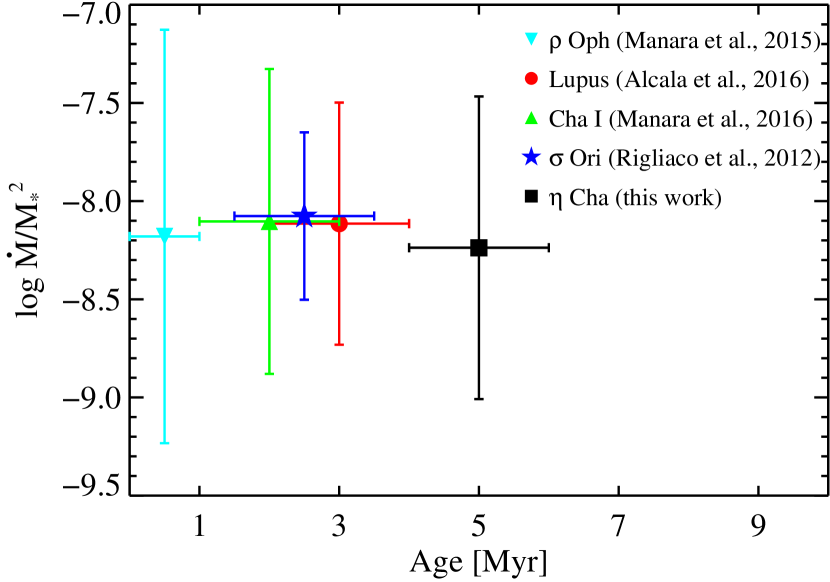
Figure 12: Mass accretion rates normalized by stellar mass squared at cluster ages of individual star forming regions. The mass accretion rate $\dot{M}$ of each star has been divided by $M_{*}^{2}$ and combined by the median for each cluster. $\dot{M}$ is given in units of ${\rm M_{\sun}/yr}$ and the stellar mass $M_{\rm*}$ is given in units of ${\rm M_{\sun}}$. Stars in the $\eta$ Cha association are shown as a filled black square. The other clusters are shown as a cyan inverted triangle for $\rho$ Ophiucus, as a red circle for Lupus, as a green triangle for Chamaeleon I and as a blue star for $\sigma$ Orionis. The error bars indicate the standard deviation in logarithmic scale of the normalized mass accretion rates.

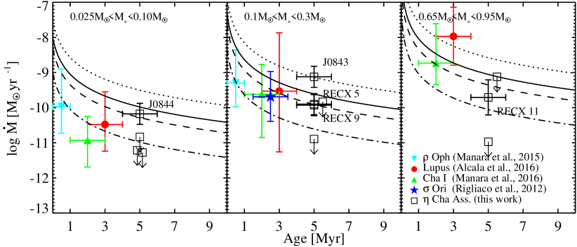
Figure 13: Mass accretion rate versus cluster age for three different stellar mass ranges. The ranges are indicated in each panel. Stars in the $\eta$ Cha association are shown as empty black squares. Upper limits are drawn as arrows for objects with no detected accretion, otherwise, colors and symbols as in Fig. 12. The dotted, solid, dashed and dashed-dotted lines indicate fiducial models for viscous accretion with disk masses of 30%, 10%, 5% and 1% of the mass of the central star, respectively. The stellar mass used in the model is $M_{*}=0.05\,{\rm M_{\sun}}$ in the left, $M_{*}=0.15\,{\rm M_{\sun}}$ in the middle and $M_{*}=0.8\,{\rm M_{\sun}}$ in the right panel (see details and references in text).

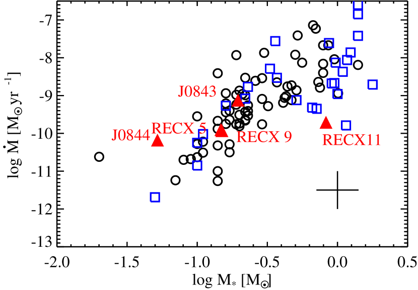
Figure 14: Mass accretion rate vs. stellar mass for objects in the $\eta$ Cha cluster (red filled triangles; this work), the Lupus (black empty circles; Alcalá et al. 2017) and Chamaeleon I star forming regions (blue empty squares; Manara et al. 2016). Note that RECX 5 and RECX 9 overlap in this presentation, as they differ only slightly in stellar mass and mass accretion rate. In the lower-right corner, typical errors are indicated.

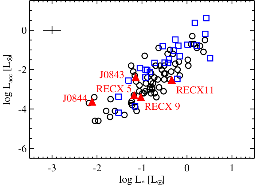
Figure 15: Accretion luminosity vs. stellar mass for objects in the $\eta$ Cha cluster (red filled triangles; this work), the Lupus (black empty circles; Alcalá et al. 2017) and Chamaeleon I star forming regions (blue empty squares; Manara et al. 2016). In the upper-left corner, typical errors are indicated.

6.3 Comparisons to other low mass star forming regions

Figures 14 and 15 compare the UV-excess measurements of $L_{\rm acc}$ and $\dot{M}$ of $\eta$ Cha members with those measured onto stars in the Lupus and Chamaeleon I star forming regions (Alcalá et al., 2014, 2017; Manara et al., 2016). The locus of $\eta$ Cha objects is consistent with accretors in other regions. Therefore, the accretion properties appear to be similar.

To support this conclusion, we compare the mass accretion rates of the $\eta$ Cha association to those of other clusters with different ages. The measurements have been compiled from the literature for the $\rho$ Ophiucus (Manara et al., 2015), Lupus (Alcalá et al., 2017), Chamaeleon I (Manara et al., 2016) and $\sigma$ Orionis (Rigliaco et al., 2011) star forming regions. These clusters have been selected because the mass accretion rates were determined with a similar technique (except for $\rho$ Ophiucus, for which $\dot{M}$ was determined from emission lines; Manara et al. 2015) and the observations were conducted with the same instrument (X-Shooter). We adopt cluster ages of 0.5 Myr for $\rho$ Ophiucus (Greene & Meyer, 1995; Luhman & Rieke, 1999; Mohanty et al., 2005), 2 Myr for Chamaeleon I, 2.5 Myr for $\sigma$ Orionis (both Fang et al., 2013, and references therein) and 3 Myr for Lupus (Alcalá et al., 2014, 2017), and 5 Myr for the $\eta$ Cha Association. The accretion rate for each star is normalized by the relationship $\dot{M}\propto M_{*}^{2.0}$ (based on previous estimates with an exponent $\sim 2.0$ from, e.g., Hartmann et al., 2016; Manara et al., 2017).

The median mass accretion rates agree well for all clusters, despite differences in age (Figure 12). Disk dispersal is expected to be governed by viscous accretion at least in some phases of its evolution, which implies a decrease of mass accretion rate with time (e.g., Hartmann et al., 1998; Alexander et al., 2014). Among stars with ongoing accretion, the decrease in accretion rate with time is not detected.

However, drawing conclusions on the physical description of disk accretion from these comparisons is challenging for several reasons (see also, Manara et al., 2016; Hartmann et al., 2016): first, while the average accretion rate may not change, the fraction of stars with disks and with ongoing accretion decreases with time (e.g. Haisch et al., 2001; Hernández et al., 2008; Fedele et al., 2010); second, stars in a single cluster may have an age spread, in which case the stars with disks may be younger than the average cluster age; finally, according to models of viscous accretion, the change in accretion rate with stellar age will flatten out, i.e., will decrease with stellar age (e.g., Hartmann et al., 1998). The $\eta$ Chamaeleontis cluster may therefore be biased towards higher initial disk masses, as these live longer than their lower mass counterparts. Comparisons to clusters at older ages to younger ones is therefore difficult (Sicilia-Aguilar et al., 2010). This effect may be enhanced by the possible onset of photo-evaporation, which could quickly remove disks once the mass accretion rate drops below about $10^{-10}{\,}{\rm M_{\sun}/yr}$ for solar-mass stars (Clarke et al., 2001; Gorti et al., 2009).

We therefore investigate how accretion rates of similar-mass stars compare among clusters of different age, and how they relate to models of viscous evolution (Figure 13). As the $\eta$ Cha association hosts only five accreting objects, which span an order of magnitude in stellar mass, the cluster samples are divided into three mass bins and each $\eta$ Cha object is drawn separately. The mass ranges have been chosen around the mass of J0844 ($0.025<M_{\sun}<0.1$; left panel), of J0843, RECX 5 and RECX 9 ($0.1<M_{\sun}<0.3$; middle panel), and of RECX 11 ($0.65<M_{\sun}<0.95$; right panel). For the clusters, the mean in logarithmic scale of $\dot{M}$ is given. It is only shown, if a single mass bin contained at least 3 objects. The error bars of $\dot{M}$ are the minimum and maximum accretion rate in each mass bin. While upper limits on $\dot{M}$ are drawn as arrows for non-accreting objects in the $\eta$ Cha association, upper limits have not been included for other clusters.

Fiducial models of accretion by viscous evolution (Hartmann et al., 1998) are for stellar masses of $0.05$, $0.15$, and $0.8$ M_☉, with initial disk masses of 30%, 10%, 5% and 1% times the mass of the central star. This simple parametric model assumes $\alpha=10^{-2}$, $R_{1}=10{\rm\leavevmode\nobreak\ AU}$ and $T_{\rm 100AU}=10{\,}{\rm K}$ (see Hartmann et al. 1998 for more details on the parameters).

In the lowest mass bin, the time evolution of accretion between $\rho$ Ophiucus and Lupus and Chamaeleon I is traced well by a viscous accretion model with $M_{*}=0.05\,M_{\sun}$ and a disk mass of $M_{\rm disk}=0.005\,M_{\sun}$ (dashed-dotted model in the left panel of Fig. 13). At the age of the $\eta$ Cha cluster, mass accretion rates expected from this model would be below the detection limit of the method presented here, as indicated by the upper limits of non-accreting objects. On the other hand, $\dot{M}$ of J0844 lies on the high end of the range of mass accretion rates found in the Lupus and Chamaeleon I, which could be explained if J0844 had a high initial disk mass. J0843 also shows an enhanced accretion rate.

RECX 5 and RECX 9 are accreting at rates that are lower but within the range of accretion rates in Lupus, Chamaeleon I, and $\sigma$ Orionis. This difference is in agreement with viscous accretion models. RECX 11 shows significantly lower $\dot{M}$ than seen in other clusters for stars of similar mass. In direct comparison to Chamaeleon I, this difference is in agreement with expectations from simple models of viscous disk accretion (see Fig. 13).

7 Conclusions

We present a revised analysis of the mass accretion and stellar properties of 15 low-mass stars in the nearby $\eta$ Cha association. Thanks to the simultaneous, broad-wavelength-range coverage and flux-calibration accuracy of VLT/X-Shooter we determined the spectral type, extinction and accretion luminosity in a self-consistent way. Out of the 15 low-mass stars studied here, we detected ongoing mass accretion in 5 systems. Once compared with literature values, we find that the mass accretion rates are consistent within errors with previous studies for which UV excess measurements exist, and deviating for most objects, when comparing to results from H$\alpha$ modeling due to methodological differences. We also report a mass accretion rate for J0844, for which no direct measurement of mass accretion has been reported in the literature. The derived mass accretion rates in the $\eta$ Cha cluster are similar to the values measured in younger star forming regions.

Appendix A Spectra and best-fit models of accretors in the $\eta$ Cha cluster

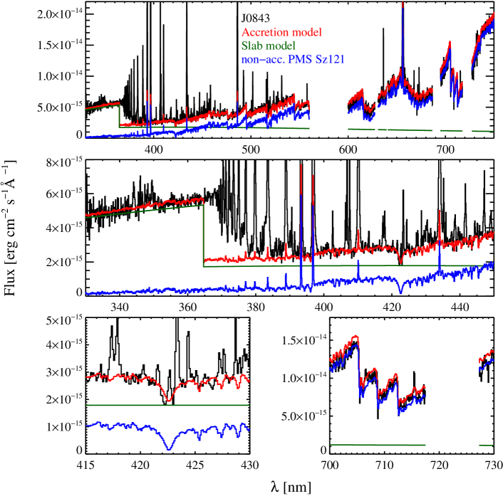
Figure 16: Accretion model (red) of PMS J0843 (black), using as basis the non-accreting PMS Sz121 (blue; Manara et al. 2013b) and a plane parallel Hydrogen slab (green; Valenti et al. 1993). The spectra have been re-binned to 0.1 nm resolution.

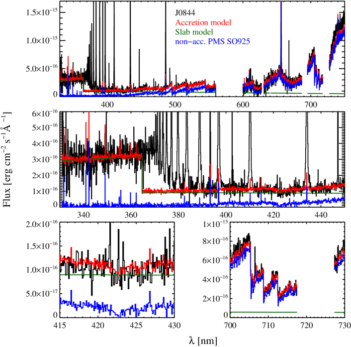
Figure 17: Accretion model of PMS J0844, using as basis the non-accreting PMS SO925 (Manara et al. 2013b). Colors as in Fig. 16.

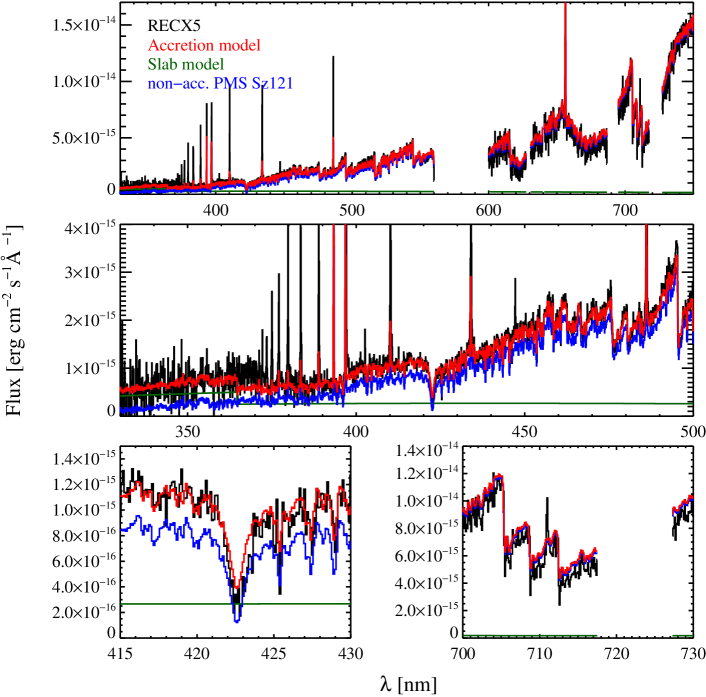
Figure 18: Accretion model to PMS RECX5, using as basis the non-accreting PMS Sz121 (Manara et al. 2013b). Colors as in Fig. 16.

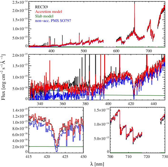
Figure 19: Accretion model to PMS RECX 9, using as basis the non-accreting PMS SO797 (Manara et al. 2013b). Colors as in Fig. 16. The spectra have been re-binned to 0.2 nm resolution.

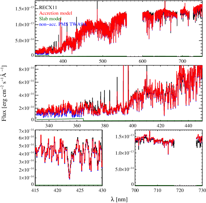
Figure 20: Accretion model to PMS RECX 11, using as basis the non-accreting PMS TWA9A (Manara et al. 2013b). Colors as in Fig. 16.

In Figures 16-20, the accreting PMSs in the $\eta$ Cha cluster are shown together with the models, which were used to determine the accretion flux.

Appendix B Emission lines

We report flux and equivalent width of the H$\alpha$ and H$\beta$ transitions, the He i${\leavevmode\nobreak\ \lambda 402.6}$, ${{\rm HeI}\leavevmode\nobreak\ \lambda 447.1}$, He i${\leavevmode\nobreak\ \lambda 501.5}$, He i${\leavevmode\nobreak\ \lambda 587.5}$, He i${\leavevmode\nobreak\ \lambda 667.8}$, He i${\leavevmode\nobreak\ \lambda 706.5}$ transitions and the ${\rm HeIFeI}\lambda 492.2$ emission feature (Alcalá et al. 2014). We include the detections of the [O i]${\leavevmode\nobreak\ \lambda 557.7}$, [O i]${\leavevmode\nobreak\ \lambda 630.0}$ and [O i]${\leavevmode\nobreak\ \lambda 636.3}$ forbidden transitions.

Table 7: Fluxes and equivalent widths of forbidden Oxygen transitions

Object	$f_{{\rm[OI]}\leavevmode\nobreak\ \lambda 557.7}$	$EW_{{\rm[OI]}\leavevmode\nobreak\ \lambda 557.7}$	$f_{{\rm[OI]}\leavevmode\nobreak\ \lambda 630.0}$	$EW_{{\rm[OI]}\leavevmode\nobreak\ \lambda 630.0}$	$f_{{\rm[OI]}\leavevmode\nobreak\ \lambda 636.3}$	$EW_{{\rm[OI]}\leavevmode\nobreak\ \lambda 636.3}$
	[${\rm erg}{\rm s}^{-1}{\rm cm}^{-2}$]	[Å]	[${\rm erg}{\rm s}^{-1}{\rm cm}^{-2}$]	[Å]	[${\rm erg}{\rm s}^{-1}{\rm cm}^{-2}$]	[Å]
J0836	¡9.56e-18	-	¡2.92e-17	-	¡5.84e-17	-
RECX1	¡1.24e-14	-	¡9.35e-15	-	¡6.00e-15	-
J0838	¡3.63e-17	-	¡1.26e-16	-	¡1.72e-16	-
J0841	¡1.30e-17	-	6.65($\pm$0.93)e-16	-1.18$\pm$0.18	¡6.42e-17	-
RECX3	¡1.62e-16	-	¡3.61e-16	-	¡5.48e-16	-
RECX4	¡9.36e-16	-	¡1.14e-15	-	¡1.08e-15	-
RECX5	9.34($\pm$3.45)e-16	-0.27$\pm$0.10	¡3.77e-16	-	¡4.85e-16	-
RECX6	¡3.03e-16	-	¡3.26e-16	-	¡4.46e-16	-
RECX7	¡5.86e-15	-	¡5.63e-15	-	¡9.11e-15	-
J0843	6.94($\pm$0.47)e-15	-1.27$\pm$0.08	7.18($\pm$0.32)e-14	-12.91$\pm$0.48	2.40($\pm$0.20)e-14	-3.62$\pm$0.35
J0844	1.35($\pm$0.51)e-16	-0.73$\pm$0.30	¡4.04e-17	-	¡6.13e-17	-
RECX9	1.64($\pm$0.29)e-15	-0.47$\pm$0.09	¡2.98e-16	-	¡3.95e-16	-
RECX10	¡1.66e-15	-	¡1.86e-15	-	¡1.59e-15	-
RECX11	¡5.16e-15	-	¡4.62e-15	-	¡2.37e-15	-

Table 8: Fluxes and equivalent widths of Helium transitions (1)

Object	$f_{{\rm HeI}\leavevmode\nobreak\ \lambda 402.6}$	$EW_{{\rm HeI}\leavevmode\nobreak\ \lambda 402.6}$	$f_{{\rm HeI}\leavevmode\nobreak\ \lambda 447.1}$	$EW_{{\rm HeI}\leavevmode\nobreak\ \lambda 447.1}$	$f_{{\rm HeI}\leavevmode\nobreak\ \lambda 501.5}$	$EW_{{\rm HeI}\leavevmode\nobreak\ \lambda 501.5}$
	[${\rm erg}{\rm s}^{-1}{\rm cm}^{-2}$]	[Å]	[${\rm erg}{\rm s}^{-1}{\rm cm}^{-2}$]	[Å]	[${\rm erg}{\rm s}^{-1}{\rm cm}^{-2}$]	[Å]
J0836	¡1.54e-17	-	1.08($\pm$0.23)e-16	-0.74$\pm$0.17	¡1.07e-17	-
RECX1	¡1.38e-14	-	¡1.27e-14	-	¡1.40e-14	-
J0838	¡4.74e-17	-	¡3.29e-17	-	¡2.40e-17	-
J0841	9.42($\pm$4.74)e-17	-0.61$\pm$0.32	¡1.32e-17	-	¡1.65e-17	-
RECX3	¡1.87e-16	-	¡1.46e-16	-	¡2.25e-16	-
RECX4	¡5.80e-16	-	¡7.96e-16	-	¡1.03e-15	-
RECX5	1.73($\pm$0.34)e-15	-2.10$\pm$0.49	2.22($\pm$0.32)e-15	-1.33$\pm$0.22	¡9.46e-17	-
RECX6	¡2.30e-16	-	¡1.71e-16	-	¡2.91e-16	-
RECX7	¡7.74e-15	-	¡8.81e-15	-	¡6.56e-15	-
J0843	6.01($\pm$0.49)e-15	-2.34$\pm$0.19	1.13($\pm$0.06)e-14	-3.09$\pm$0.14	2.34($\pm$0.11)e-14	-5.69$\pm$0.22
J0844	6.66($\pm$0.64)e-16	-5.08$\pm$0.63	1.28($\pm$0.07)e-15	-8.08$\pm$0.71	3.30($\pm$0.31)e-16	-2.27$\pm$0.24
RECX9	9.03($\pm$1.99)e-16	-0.88$\pm$0.20	1.33($\pm$0.17)e-15	-0.81$\pm$0.10	¡9.75e-17	-
RECX10	¡8.34e-16	-	¡1.26e-15	-	¡1.62e-15	-
RECX11	¡5.13e-15	-	¡5.13e-15	-	¡6.05e-15	-
RECX12	2.68($\pm$0.63)e-15	-0.52$\pm$0.13	4.69($\pm$1.23)e-15	-0.42$\pm$0.11	¡5.55e-16	-

Table 9: Fluxes and equivalent widths of Helium transitions (2)

Object	$f_{{\rm HeI}\leavevmode\nobreak\ \lambda 587.5}$	$EW_{{\rm HeI}\leavevmode\nobreak\ \lambda 587.5}$	$f_{{\rm HeI}\leavevmode\nobreak\ \lambda 667.8}$	$EW_{{\rm HeI}\leavevmode\nobreak\ \lambda 667.8}$	$f_{{\rm HeI}\leavevmode\nobreak\ \lambda 706.5}$	$EW_{{\rm HeI}\leavevmode\nobreak\ \lambda 706.5}$
	[${\rm erg}{\rm s}^{-1}{\rm cm}^{-2}$]	[Å]	[${\rm erg}{\rm s}^{-1}{\rm cm}^{-2}$]	[Å]	[${\rm erg}{\rm s}^{-1}{\rm cm}^{-2}$]	[Å]
J0836	¡7.02e-17	-	¡6.24e-17	-	¡9.36e-17	-
RECX1	¡1.08e-14	-	¡3.21e-15	-	¡4.20e-15	-
J0838	¡2.15e-16	-	¡1.64e-16	-	¡1.78e-16	-
J0841	¡9.16e-17	-	¡8.71e-17	-	¡9.63e-17	-
RECX3	¡5.20e-16	-	¡4.37e-16	-	¡9.34e-16	-
RECX4	¡1.52e-15	-	¡8.19e-16	-	¡1.87e-15	-
RECX5	4.64($\pm$1.29)e-15	-1.86$\pm$0.51	3.97($\pm$1.33)e-15	-0.95$\pm$0.38	¡4.67e-16	-
RECX6	¡5.48e-16	-	¡3.28e-16	-	¡6.29e-16	-
RECX7	¡6.53e-15	-	¡1.71e-15	-	¡3.19e-15	-
J0843	2.25($\pm$0.19)e-14	-4.70$\pm$0.35	6.37($\pm$1.24)e-15	-0.85$\pm$0.19	¡4.91e-16	-
J0844	1.45($\pm$0.22)e-15	-9.95$\pm$1.44	1.00($\pm$0.13)e-15	-4.66$\pm$1.13	6.17($\pm$1.04)e-16	-1.56$\pm$0.28
RECX9	4.76($\pm$1.03)e-15	-1.66$\pm$0.35	¡2.51e-16	-	¡4.02e-16	-
RECX10	¡1.97e-15	-	¡9.02e-16	-	¡1.84e-15	-
RECX11	¡5.20e-15	-	¡1.53e-15	-	¡2.24e-15	-
RECX12	1.43($\pm$0.19)e-14	-0.70$\pm$0.09	¡7.17e-16	-	¡1.52e-15	-

Table 10: Fluxes and equivalent widths of Helium (3), H$\alpha$ and H$\beta$ transitions

Object	$f_{{\rm HeIFeI}\leavevmode\nobreak\ \lambda 492.2}$	$EW_{{\rm HeIFeI}\leavevmode\nobreak\ \lambda 492.2}$	$f_{{\rm H\alpha}\leavevmode\nobreak\ \lambda 656.3}$	$EW_{{\rm H\alpha}\leavevmode\nobreak\ \lambda 656.3}$	$f_{{\rm H\beta}\leavevmode\nobreak\ \lambda 486.1}$	$EW_{{\rm H\beta}\leavevmode\nobreak\ \lambda 486.1}$
	[${\rm erg}{\rm s}^{-1}{\rm cm}^{-2}$]	[Å]	[${\rm erg}{\rm s}^{-1}{\rm cm}^{-2}$]	[Å]	[${\rm erg}{\rm s}^{-1}{\rm cm}^{-2}$]	[Å]
J0836	¡1.36e-17	-	1.25($\pm$0.06)e-14	-13.38$\pm$0.72	2.10($\pm$0.09)e-15	-11.13$\pm$0.37
RECX1	¡1.17e-14	-	3.19($\pm$0.27)e-13	-1.05$\pm$0.09	¡1.22e-14	-
J0838	¡2.66e-17	-	2.23($\pm$0.12)e-14	-11.98$\pm$0.77	4.19($\pm$0.20)e-15	-10.42$\pm$0.40
J0841	¡1.85e-17	-	1.10($\pm$0.06)e-14	-9.45$\pm$0.62	2.32($\pm$0.11)e-15	-8.26$\pm$0.29
RECX3	¡2.13e-16	-	3.94($\pm$0.38)e-14	-2.73$\pm$0.28	7.97($\pm$0.61)e-15	-1.91$\pm$0.14
RECX4	¡9.90e-16	-	1.85($\pm$0.11)e-13	-4.24$\pm$0.26	4.50($\pm$0.30)e-14	-2.68$\pm$0.16
RECX5	¡8.64e-17	-	8.68($\pm$0.42)e-14	-13.50$\pm$0.68	2.92($\pm$0.12)e-14	-14.70$\pm$0.35
RECX6	¡2.80e-16	-	8.93($\pm$0.47)e-14	-5.32$\pm$0.24	2.28($\pm$0.11)e-14	-4.03$\pm$0.14
RECX7	¡7.28e-15	-	1.65($\pm$0.21)e-13	-0.79$\pm$0.10	¡7.20e-15	-
J0843	2.40($\pm$0.11)e-14	-4.99$\pm$0.11	9.90($\pm$0.40)e-13	-94.45$\pm$2.63	1.75($\pm$0.07)e-13	-42.61$\pm$0.68
J0844	6.64($\pm$0.39)e-16	-3.26$\pm$0.16	4.40($\pm$0.18)e-14	-102.20$\pm$5.45	1.40($\pm$0.06)e-14	-82.07$\pm$1.98
RECX9	¡9.69e-17	-	9.60($\pm$0.43)e-14	-12.60$\pm$0.47	2.10($\pm$0.09)e-14	-10.73$\pm$0.30
RECX10	¡1.31e-15	-	9.14($\pm$1.05)e-14	-1.68$\pm$0.20	2.76($\pm$0.38)e-14	-1.15$\pm$0.16
RECX11	¡5.27e-15	-	1.16($\pm$0.05)e-12	-8.32$\pm$0.29	2.56($\pm$0.21)e-13	-2.73$\pm$0.22
RECX12	¡6.36e-16	-	3.05($\pm$0.13)e-13	-8.41$\pm$0.22	1.06($\pm$0.04)e-13	-8.15$\pm$0.16