The algorithmic structure of the finite stopping time behavior of the $3x+1$ function

Abstract

The $3x+1$ problem concerns iteration of the map $T:\mathbb{Z}\rightarrow\mathbb{Z}$ given by

$$T(x)=\left\{\begin{array}[]{lcr}\;\;\;\;\displaystyle{\frac{x}{2}}&\mbox{if \, $x\equiv 0\ (\text{mod}\ 2)$},\\ \\ \displaystyle{\frac{3x+1}{2}}&\mbox{if \, $x\equiv 1\ (\text{mod}\ 2)$}.\end{array}\right.$$

The $3x+1$ Conjecture states that every $x\geq 1$ has some iterate $T^{s}(x)=1$. The least $s\in\mathbb{N}$ such that $T^{s}(x)<x$ is called the stopping time of $x$. It is shown that the residue classes of the integers $x>1$ with a finite stopping time can be evolved according to a directed rooted tree based on their parity vectors. Each parity vector represents a unique Diophantine equation whose only positive solutions are the integers with a finite stopping time. The tree structure is based on a precise algorithm which allows accurate statements about the solutions $x$ without solving the Diophantine equations explicitly. As a consequence, the integers $x>1$ with a finite stopping time can be generated algorithmically. It is also shown that the OEIS sequences A076227 and A100982 related to the residues $(\text{mod}\ 2^{k})$ can be generated algorithmically in a Pascal’s triangle-like manner from the two starting values 0 and 1. For the results no statistical and probability theoretical methods were used.

Keywords and phrases: 3x + 1 problem, 3n + 1 conjecture, Collatz conjecture, Ulam conjecture, Kakutani’s problem, Thwaites conjecture, Hasse’s algorithm, Syracuse problem, hailstone sequence, finite stopping time, OEIS, A020914, A020915, A022921, A056576, A076227, A100982, A177789, A293308

Edits in this 3nd version: Shortened abstract, corrected typos on p.7, addition of A293308 on p.1 and p.9, corrected font for ”mod”, 2st version from Sep. 21, 2017.

1 Introduction

The $3x+1$ function is defined as a function $T:\mathbb{Z}\rightarrow\mathbb{Z}$ given by

$$T(x)=\left\{\begin{array}[]{lcr}\;\;\;\;\displaystyle{\frac{x}{2}}&\mbox{if \, $x\equiv 0\ (\text{mod}\ 2)$},\\ \\ \displaystyle{\frac{3x+1}{2}}&\mbox{if \, $x\equiv 1\ (\text{mod}\ 2)$}.\end{array}\right.$$ (4)

Let $T^{0}(x)=x$ and $T^{s}(x)=T\left(T^{s-1}(x)\right)$ for $s\in\mathbb{N}$. Then we get for each $x\in\mathbb{N}$ a sequence $C(x)=\left(T^{s}(x)\right)_{s=0}^{\infty}$.

For example the starting value $x=11$ generates the sequence

$$C(11)=(11,17,26,13,20,10,5,8,4,2,1,2,1,2,1,\dotsc).$$

Any $C(x)$ can only assume two possible forms. Either it falls into a cycle or it grows to infinity. The $3x+1$ Conjecture states that every $C(x)$ enters the trivial cycle $(2,1,2,1,\dotsc)$.

2 The stopping time $\sigma(x)$ and the residues $(\text{mod}\ 2^{k})$

The $3x+1$ Conjecture holds if for each $x\in\mathbb{N},x>1$, there exists $s\in\mathbb{N}$ such that $T^{s}(x)<x$. The least $s\in\mathbb{N}$ such that $T^{s}(x)<x$ is called the stopping time of $x$, which we will denote by $\sigma(x)$.

For the further text we define the following:

• Let $C^{a}(x)=\left(T^{s}(x)\right)_{s=0}^{a},$ $a\in\mathbb{N},a\geq 1$, be a finite subsequence of $C(x)$.

• Let $n\geq 1,n\in\mathbb{N}$, be the number of odd terms in $C^{\sigma(x)-1}(x)$, whereby $T^{0}(x)$ is not counted.

• Let $\sigma_{n}:=\lfloor 1+(n+1)\cdot\log_{2}3\rfloor$ for all $n\in\mathbb{N}$.

It is not hard to verify that for specific residue classes of starting values $x>1$ only specific stopping times $\sigma(x)$ are possible which are determined by the real number $\log_{2}3$.

Let $r_{i},z\in\mathbb{N}$, $i=1,\dotsc,z$. Then generally applies for each $n\geq 1$ that

$$\sigma(x)=\sigma_{n}\quad\text{if}\quad x\equiv r_{1},r_{2},r_{3},\dotsc,r_{z}\ (\text{mod}\ 2^{\sigma_{n}}).$$ (5)

For the first $n\geq 1$ there is

               $\sigma(x)=\sigma_{1}=4$  if   $x\equiv 3\ (\text{mod}\ 16)$,
               $\sigma(x)=\sigma_{2}=5$  if   $x\equiv 11,23\ (\text{mod}\ 32)$,
               $\sigma(x)=\sigma_{3}=7$  if   $x\equiv 7,15,59\ (\text{mod}\ 128)$,
               $\sigma(x)=\sigma_{4}=8$  if   $x\equiv 39,79,95,123,175,199,219\ (\text{mod}\ 256)$,
               
and so forth. Appendix 9.2 shows the above list up to $\sigma(x)=15$.

Let $z(n)\geq 1$ for each $n\geq 1$ be the number of residue classes $(\text{mod}\ 2^{\sigma_{n}})$, respectively the number of congruences $r_{i}$, as listed in A100982.

Theorem 1.

There exists for each $n\geq 1$ a set of $z(n)\geq 1$ residue classes $(\text{mod}\ 2^{\sigma_{n}})$ with the property that all integers $x>1$ of one of these residue classes have finite stopping time $\sigma(x)=\sigma_{n}$.

Proof. All essential references are given in the OEIS [5]. The possible stopping times $\sigma_{n}$ are listed in A020914. The congruences $r_{i}$ of the associated residue classes $(\text{mod}\ 2^{\sigma_{n}})$ are listed in A177789. But the proof of Theorem 2 is also a proof of Theorem 1. $\square$

Remarkably, as we shall see in the course of the next pages, the residue classes $(\text{mod}\ 2^{\sigma_{n}})$ as mentioned in Theorem 1 can be generated algorithmically according to a directed rooted tree. (cf. Chapter 8)

Theorem 2.

For each $n\geq 3$ the number of residue classes $(\text{mod}\ 2^{\sigma_{n}})$ as listed in A100982 and the number of the remaining residue classes $(\text{mod}\ 2^{k})$ as listed in A076227 can be generated algorithmically in a Pascal’s triangle-like manner from the two starting values 0 and 1.

Proof. The residues $(\text{mod}\ 2^{k})$ can be evolved according to a binary tree. For the residues $(\text{mod}\ 2^{k})$ in each case, $k$ steps can be calculated. As long as a factor 2 is included, only the residue decides whether the next number is even or odd, and this step can be performed. If the powers of 2 are dissipated, they are replaced by a certain number of factors 3, which is less than or equal to the initial $k$, depending on how many $\frac{3x+1}{2}$ and $\frac{1}{2}$ steps have occurred.

Let $r,q\in\mathbb{N}$, then in general $r\ (\text{mod}\ 2^{k})$ leads to $q\ (\text{mod}\ 3^{n})$ with $k\geq n$. Whereby it is $k=n$ exactly for $r=2^{k}-1$, which is also the deeper reason for the fact that more and more residues remain, specifically the residues of the form $2^{k}-1$. If $2^{k}>3^{n}$ then the sequence can be sorted out, because the stopping time is reached.

If we now pass from a specific value $k$ to the value $k+1$, always two new values arise from the remaining candidates, so $r\ (\text{mod}\ 2^{k})$ became $r\ (\text{mod}\ 2^{k+1})$ or $(r+2^{k})\ (\text{mod}\ 2^{k+1})$. For one of them the result in the $k$-th step is even, for the other it is odd. Which is what, we did not know before doubling the base, which is why we had to stop. And accordingly one continues with the $\frac{3x+1}{2}$ step and thus to a value of the power of 3 increased by one, and the other with the $\frac{1}{2}$ step while maintaining the power of 3.

Now we consider the number of residues that lead to a specific power of 3. Let $\mathcal{R}(k,n)$ be the number of residues $(\text{mod}\ 2^{k})$ which meet the condition $2^{k}<3^{n}$ and lead to a residue $(\text{mod}\ 3^{n})$. Each residue $(\text{mod}\ 2^{k+1})$ comes from a residue $(\text{mod}\ 2^{k})$, and either $n$ is increased or $n$ is retained, depending on the type of step performed. Thus we have

$$\mathcal{R}(k+1,n)=\mathcal{R}(k,n)+\mathcal{R}(k,n-1)$$ (6)

with the starting condition $\mathcal{R}(2,2)=1$ and $\mathcal{R}(2,1)=0$. Because $3\ (\text{mod}\ 2^{2})$ is the only non-trivial staring value and leads to $8\ (\text{mod}\ 3^{2})$. As a consequence, the number of residues $(\text{mod}\ 2^{k})$ can be calculated in a Pascal’s triangle-like manner or form, whose left side is cut off by the stopping time condition $2^{k}>3^{n}$. The number of $2^{k}$ between $3^{n-1}$ and $3^{n}$, as listed in A022921, we will denote by $d(n)$, is given by

$$d(n)=\lfloor n\cdot\log_{2}3\rfloor-\lfloor(n-1)\cdot\log_{2}3\rfloor.$$ (7)

The highest $k$ such that $2^{k}<3^{n}$, as listed in A056576, we will denote by $\kappa(n)$ for each $n\geq 2$. Then with equation (7) it is

$$\kappa(n)=\sum_{i=1}^{n}d(i)=\sum_{i=1}^{n}\Big{(}\lfloor i\cdot\log_{2}3\rfloor-\lfloor(i-1)\cdot\log_{2}3\rfloor\Big{)},$$ (8)

and from the above definition of $\kappa(n)$ it follows also directly that

$$\kappa(n)=\lfloor n\cdot\log_{2}3\rfloor.$$ (9)

Further it is $\kappa(n)+1=\lfloor 1+n\cdot\log_{2}3\rfloor=\lfloor 1+((n-1)+1)\cdot\log_{2}3\rfloor$. Then with $\sigma_{n}=\lfloor 1+(n+1)\cdot\log_{2}3\rfloor$ we get $\kappa(n)+1=\sigma_{n-1}$ with is equivalent to

$$\kappa(n+1)+1=\sigma_{n}.$$ (10)

Equation (10) states that $\kappa(n+1)+1$ is the stopping time for $x>1$ for each $n\in\mathbb{N}$, which completes the circle to (5) and Theorem 1. Remember that $n\geq 1$ is the number of odd terms in $C^{\sigma(x)-1}(x)$, whereby $T^{0}(x)$ is not counted. Therefore the stopping time $\sigma(x)$ for each $n\geq 1$ is given exactly by $k+1$ of the highest $k$ such that $2^{k}<3^{n+1}$ or $\kappa(n+1)+1$.

Back to the left sided bounding condition: For each $n\geq 2$ the last value $\mathcal{R}(k+1,n)$ of equation (6) is given by

$$k+1=\kappa(n).$$ (11)

With the use of (6), (7), (8) and (11) now we are able to create an algorithm which generates A100982 and A076227 from the two starting values 0 and 1 for each $n\geq 3$. $\square$

Appendix 9.1.1 and 9.1.2 show a program for the algorithm of Theorem 2. Appendix 9.3 shows a detailed list for the expansion of the first residue classes $(\text{mod}\ 2^{k})$.

Table 1 will make the algorithm of Theorem 2 more clear, no entry is equal to 0.

$d(n)=$	1	2	1	2	1	2	2	1	2	1	2	$\cdots$
${\color[rgb]{0.0,0.5,0.0}n=}$	${\color[rgb]{0.0,0.5,0.0}1}$	${\color[rgb]{0.0,0.5,0.0}2}$	${\color[rgb]{0.0,0.5,0.0}3}$	${\color[rgb]{0.0,0.5,0.0}4}$	${\color[rgb]{0.0,0.5,0.0}5}$	${\color[rgb]{0.0,0.5,0.0}6}$	${\color[rgb]{0.0,0.5,0.0}7}$	${\color[rgb]{0.0,0.5,0.0}8}$	${\color[rgb]{0.0,0.5,0.0}9}$	${\color[rgb]{0.0,0.5,0.0}10}$	${\color[rgb]{0.0,0.5,0.0}11}$	${\color[rgb]{0.0,0.5,0.0}\cdots}$
${\color[rgb]{0.6,0.0,0.8}k=}$													${\color[rgb]{0.8,0.3,0.0}w(k)=}$
${\color[rgb]{0.6,0.0,0.8}2}$		1											${\color[rgb]{0.8,0.3,0.0}1}$
${\color[rgb]{0.6,0.0,0.8}3}$		1	1										${\color[rgb]{0.8,0.3,0.0}2}$
${\color[rgb]{0.6,0.0,0.8}4}$			2	1									${\color[rgb]{0.8,0.3,0.0}3}$
${\color[rgb]{0.6,0.0,0.8}5}$				3	1								${\color[rgb]{0.8,0.3,0.0}4}$
${\color[rgb]{0.6,0.0,0.8}6}$				3	4	1							${\color[rgb]{0.8,0.3,0.0}8}$
${\color[rgb]{0.6,0.0,0.8}7}$					7	5	1						${\color[rgb]{0.8,0.3,0.0}13}$
${\color[rgb]{0.6,0.0,0.8}8}$						12	6	1					${\color[rgb]{0.8,0.3,0.0}19}$
${\color[rgb]{0.6,0.0,0.8}9}$						12	18	7	1				${\color[rgb]{0.8,0.3,0.0}38}$
${\color[rgb]{0.6,0.0,0.8}10}$							30	25	8	1			${\color[rgb]{0.8,0.3,0.0}64}$
${\color[rgb]{0.6,0.0,0.8}11}$							30	55	33	9	1		${\color[rgb]{0.8,0.3,0.0}128}$
${\color[rgb]{0.6,0.0,0.8}\vdots}$								$\vdots$	$\vdots$	$\vdots$	$\vdots$	$\ddots$	${\color[rgb]{0.8,0.3,0.0}\vdots}$
${\color[rgb]{0.0,0.3,1.0}z(n)=}$		${\color[rgb]{0.0,0.3,1.0}2}$	${\color[rgb]{0.0,0.3,1.0}3}$	${\color[rgb]{0.0,0.3,1.0}7}$	${\color[rgb]{0.0,0.3,1.0}12}$	${\color[rgb]{0.0,0.3,1.0}30}$	${\color[rgb]{0.0,0.3,1.0}85}$	${\color[rgb]{0.0,0.3,1.0}173}$	${\color[rgb]{0.0,0.3,1.0}476}$	${\color[rgb]{0.0,0.3,1.0}961}$	${\color[rgb]{0.0,0.3,1.0}2652}$	${\color[rgb]{0.0,0.3,1.0}\cdots}$

Table 1: Triangle expansion of the number of residues (mod $2^{k}$).

From Table 1 it can be seen that the sum of the values in each row $k$ is equal to the number of the surviving residues $(\text{mod}\ 2^{k})$ as listed in A076227, which we will denote by $w(k)$ for each $k\geq 2$. Then there is

$$w(k)=\sum_{n=\lfloor 1+k\cdot\log_{3}2\rfloor}^{k}\mathcal{R}(k,n).$$ (12)

The values for $\lfloor 1+k\cdot\log_{3}2\rfloor$ are listed in A020915. For example in the row for $k=6$ it can be seen that relating to $2^{6}=64$ there exist exactly $3+4+1=8$ remaining residues from which three lead to $3^{4}$, four lead to $3^{5}$ and one leads to $3^{6}$. The values with smaller powers of 3 are cut off by the condition $2^{6}=64>3^{3}=27$.

The sum of the values in each column $n$ is equal to the number of residue classes $z(n)$ as listed in A100982. With the use of equation (8) there is

$$z(n)=\sum_{k=n}^{\kappa(n)}\mathcal{R}(k,n).$$ (13)

For example in the column for $n=4$ it can be seen that there exists exactly $3+3+1=7$ residues classes $(\text{mod}\ 2^{\sigma_{n}})$ which have stopping time $\sigma_{4}=\lfloor 1+(4+1)\cdot\log_{2}3\rfloor=8$.

The exact values for $k$ of the number of $2^{k}$ between $3^{n-1}$ and $3^{n}$ as listed in A022921 are given by the largest values in each column $n$, precisely by $\kappa(n)$ and $\kappa(n)-1$. For example in the column for $n=4$ the largest values are 3 for $k=5$ and $k=6$. So, the powers of 2 existing between $3^{3}$ and $3^{4}$ are $2^{5}$ and $2^{6}$. For $n=5$ the largest value is 7 for $k=7$. Also exists only one power of 2 between $3^{4}$ and $3^{5}$ and that is $2^{7}$.

3 Subsequences $C^{\kappa(n)}(x)$ and a stopping time term formula for odd $x$

If an odd starting value $x>1$ has stopping time $\sigma(x)=\sigma_{n}$ (cf. Theorem 1) then it is shown in the proof of Theorem 2 that for each $n\geq 1$ the subsequence $C^{\kappa(n)}(x)$ represents sufficiently the stopping time of $x$. Because $C^{\kappa(n)}(x)$ consists of $n+1$ odd terms and therefore all terms $T^{s}(x)$ with $\kappa(n)<s<\sigma(x)$ are even.

If the succession of the even and odd terms in $C^{\kappa(n)}(x)$ is known, it is quite easy to develop a formula for the exact value of $T^{\sigma(x)}(x)$ with $\sigma(x)=\sigma_{n}$.

Theorem 3.

Given $C^{\kappa(n)}(x)$ consisting of $n+1$ odd terms. Let $\alpha_{i}\in\mathbb{N},\alpha_{i}\geq 0$, $i=1,\dots,n+1$. Now let $\alpha_{i}=s$, if and only if $T^{s}(x)$ in $C^{\kappa(n)}(x)$ is odd. Then there is

$$T^{\sigma_{n}}(x)=\frac{3^{n+1}}{2^{\sigma_{n}}}\cdot x+\sum_{i=1}^{n+1}\frac{3^{n+1-i}2^{\alpha_{i}}}{2^{\sigma_{n}}}<x.$$ (14)

Proof. With the use of Theorem 1 and 2, Theorem 3 follows almost directly from the $3x+1$ function (4). A detailed proof is given by the author in an earlier article [14, pp.3-4,p.9]. A similar formula is also mentioned by Garner [2, p.2]. $\square$

Example: For $n=3$ there is $\sigma_{3}=\lfloor 1+(3+1)\cdot\log_{2}3\rfloor=7$. Then for $x=59$ we get by equation (14)

$$T^{7}(59)=\frac{3^{4}}{2^{7}}\cdot 59+\frac{3^{3}2^{0}+3^{2}2^{1}+3^{1}2^{3}+3^{0}2^{4}}{2^{7}}=38<59.$$

Explanation: For $n=3$ there is $\kappa(3)=4$ and $C^{4}(59)=(59,89,134,67,101)$ consists of $3+1=4$ odd terms $59,89,67,101$. The powers of two $\alpha_{i}$ yield as follows: $T^{0}=59$ is odd, so $\alpha_{1}=0$. $T^{1}=89$ is odd, so $\alpha_{2}=1$. $T^{2}=134$ is even, so nothing happen. $T^{3}=67$ is odd, so $\alpha_{3}=3$. $T^{4}=101$ is odd, so $\alpha_{4}=4$. And a comparison with $C^{7}(59)=(59,89,134,67,101,152,76,38)$ confirms the solution $T^{7}(59)=38$. Note that there is $\sigma(x)=7$ not only for $x=59$, but also for every $x\equiv 59\ (\text{mod}\ 2^{7})$.

4 Parity vectors $v_{n}(x)$ and parity vector sets $\mathbb{V}(n)$ for each $n\geq 1$

To simplify the distribution of the even and odd terms in $C^{\kappa(n)}(x)$ we define a zero-one sequence $v_{n}(x)$ by

$$v_{n}(x)=C^{\kappa(n)}(x)\quad\text{with}\quad T^{s}(x)=\left\{\begin{array}[]{lcr}\displaystyle{0}&\mbox{if \, $T^{s}(x)\equiv 0\ (\text{mod}\ 2)$},\\ \\ \displaystyle{1}&\mbox{if \, $T^{s}(x)\equiv 1\ (\text{mod}\ 2)$},\end{array}\right.$$ (18)

which we will denote as the parity vector of $x$. In other words, $v_{n}(x)$ is a vector of $\kappa(n)+1$ elements, where ”0” represents an even term and ”1” represents an odd term in $C^{\kappa(n)}(x)$. And for each $n\geq 1$ we will define the parity vector set $\mathbb{V}(n)$ as the set of $z(n)\geq 1$ parity vectors $v_{n}(x)$, whereby $\sigma(x)=\sigma_{n}$ for each parity vector of the set. (cf. Theorem 1)

Example: For $n=3$ there is $\kappa(3)=4$. Then for $x=7$, $x=15$ and $x=59$ the subsequences $C^{\kappa(n)}(x)$ and its appropriate parity vectors $v_{n}(x)$ are

$$C^{4}(7) =(7,11,17,26,13)\quad\quad\;\;\text{has parity vector} v_{3}(7) =(1,1,1,0,1),$$

$$C^{4}(15) =(15,23,35,53,80)\quad\quad\text{has parity vector} v_{3}(15) =(1,1,1,1,0),$$

$$C^{4}(59) =(59,89,134,67,101)\quad\text{has parity vector} v_{3}(59) =(1,1,0,1,1).$$

The parity vector set $\mathbb{V}(3)$ then consists of these three parity vectors, because for $n=3$ there is $\sigma(x)=\sigma_{3}=7$ only for the $z(3)=3$ residue classes $7,15,59\ (\text{mod}\ 2^{7})$. So we have

$$\mathbb{V}(3):=\left\{\begin{array}[]{rcl}(1,1,0,1,1)\\ (1,1,1,0,1)\\ (1,1,1,1,0)\end{array}\right\}.$$

Remark 4.

According to Theorem 3, for each $n\geq 1$ there exists for each parity vector of $\mathbb{V}(n)$ with equation (14) a unique Diophantine equation

$$y=\frac{3^{n+1}}{2^{\sigma_{n}}}\cdot x+\sum_{i=1}^{n+1}\frac{3^{n+1-i}2^{\alpha_{i}}}{2^{\sigma_{n}}},$$ (19)

whose only positive integer solutions $(x,y)$ are for $x$ the residue classes $(\text{mod}\ 2^{\sigma_{n}})$ mentioned in Theorem 1. Note that the positive integer solutions $x<2^{\sigma_{n}}$ of equation (19) for each parity vector of $\mathbb{V}(n)$ are equal to the congruences $r_{i}$ as listed in A177789.

Appendix 9.4 shows the first parity vector sets $\mathbb{V}(n)$ with its integer solution $(x,y)$.

5 Generating the parity vectors of $\mathbb{V}(n)$ for each $n\geq 2$

With our results so far we are able to build the parity vectors of $\mathbb{V}(n)$ for each $n\geq 2$.

Theorem 5.

For each $n\geq 2$ the parity vectors of $\mathbb{V}(n)$ can be evolved algorithmically according to a directed rooted tree from the parity vector of $\mathbb{V}(1)$.

Proof. The initial value is the parity vector of $\mathbb{V}(1)$. Each parity vector of $\mathbb{V}(n)$ consists of $(n+1)$ 1-elements and $\big{(}\kappa(n)-n\big{)}$ 0-elements. As mentioned in the proof of Theorem 2 for each further $n$ there will be $d(n)$ steps added. Because $d(n)$ can only attain two different values, 1 or 2, the possibilities for the further parity vectors are precisely defined by these three-step-algorithm:

1. Build one new vector of $\mathbb{V}(n)$ by adding the vector of $\mathbb{V}(n-1)$ on the right side by ”$1$” if $d(n)=1$ and ”$0,1$” if $d(n)=2$.

2. Build $j\geq 1$ new vectors of $\mathbb{V}(n)$, if the new vector in step 1 contains $j\geq 1$0-elements in direct progression from the right-sided penultimate position to the left. In this case the last right-sided 1-element will change its position with each of its $j\geq 1$ left-sided 0-elements in direct progression, only one change for each new vector from the right to the left.

3. Repeat step 1 and step 2 until the new vector of $\mathbb{V}(n)$ begins with $(n+1)$ 1-elements followed by $\big{(}\kappa(n)-n\big{)}$ 0-elements.

The above algorithm produces a directed rooted tree with two different directions, a horizontal and vertical, as seen in Figure 1. This construction principle gives the tree a triangular form which extends ever more downwards with each column.

Figure 1: Tree construction principle

Figure 2 shows the beginning of the tree produced by the algorithm of Theorem 5 using the above construction principle. Each column of this tree show the parity vectors of $\mathbb{V}(n)$.  

Figure 2: Directed rooted tree for the parity vectors up to $\mathbb{V}(4)$.

Appendix 9.1.3 and 9.1.4 show a program for the algorithm of Theorem 5. Appendix 9.5 shows the tree of Figure 2 up to $\mathbb{V}(6)$. Appendix 9.6 shows an ordered list of the parity vectors of $\mathbb{V}(6)$ with its integer solution $(x,y)$ and $h$. $\square$

Now let $h\geq 2$ be the number of the first 1-elements in direct progression in a parity vector and let $\mathcal{P}(h,n)$ be the number of parity vectors for each $n\geq 1$ with $h\geq 2$ first 1-elements in direct progression. Table 2 shows the values for $\mathcal{P}(h,n)$ as generated by the algorithm of Theorem 5. The triangle structure follows directly from the construction principle of the tree. Note the peculiarity here that the first three rows are identical for each $n\geq 3$. The values of Table 2 or $\mathcal{P}(h,n)$ can also be generated in a slightly complicated Pascal’s triangle-like manner as shown by the program in Appendix 9.1.5.

${\color[rgb]{0.0,0.5,0.0}n=}$	${\color[rgb]{0.0,0.5,0.0}1}$	${\color[rgb]{0.0,0.5,0.0}2}$	${\color[rgb]{0.0,0.5,0.0}3}$	${\color[rgb]{0.0,0.5,0.0}4}$	${\color[rgb]{0.0,0.5,0.0}5}$	${\color[rgb]{0.0,0.5,0.0}6}$	${\color[rgb]{0.0,0.5,0.0}7}$	${\color[rgb]{0.0,0.5,0.0}8}$	${\color[rgb]{0.0,0.5,0.0}9}$	${\color[rgb]{0.0,0.5,0.0}10}$	${\color[rgb]{0.0,0.5,0.0}11}$	${\color[rgb]{0.0,0.5,0.0}\cdots}$
${\color[rgb]{0.6,0.0,0.8}h=}$
${\color[rgb]{0.6,0.0,0.8}2}$	1	1	1	2	3	7	19	37	99	194	525	$\cdots$
${\color[rgb]{0.6,0.0,0.8}3}$		1	1	2	3	7	19	37	99	194	525	$\cdots$
${\color[rgb]{0.6,0.0,0.8}4}$			1	2	3	7	19	37	99	194	525	$\cdots$
${\color[rgb]{0.6,0.0,0.8}5}$				1	2	5	14	28	76	151	412	$\cdots$
${\color[rgb]{0.6,0.0,0.8}6}$					1	3	9	19	53	108	299	$\cdots$
${\color[rgb]{0.6,0.0,0.8}7}$						1	4	10	30	65	186	$\cdots$
${\color[rgb]{0.6,0.0,0.8}8}$							1	4	14	34	103	$\cdots$
${\color[rgb]{0.6,0.0,0.8}9}$								1	5	15	50	$\cdots$
${\color[rgb]{0.6,0.0,0.8}10}$									1	5	20	$\cdots$
${\color[rgb]{0.6,0.0,0.8}11}$										1	6	$\cdots$
${\color[rgb]{0.6,0.0,0.8}12}$											1	$\cdots$
${\color[rgb]{0.6,0.0,0.8}\vdots}$												$\ddots$
${\color[rgb]{0.0,0.3,1.0}z(n)=}$	${\color[rgb]{0.0,0.3,1.0}1}$	${\color[rgb]{0.0,0.3,1.0}2}$	${\color[rgb]{0.0,0.3,1.0}3}$	${\color[rgb]{0.0,0.3,1.0}7}$	${\color[rgb]{0.0,0.3,1.0}12}$	${\color[rgb]{0.0,0.3,1.0}30}$	${\color[rgb]{0.0,0.3,1.0}85}$	${\color[rgb]{0.0,0.3,1.0}173}$	${\color[rgb]{0.0,0.3,1.0}476}$	${\color[rgb]{0.0,0.3,1.0}961}$	${\color[rgb]{0.0,0.3,1.0}2652}$	${\color[rgb]{0.0,0.3,1.0}\cdots}$

Table 2: Triangle expansion of the number of parity vectors regarding to their first 1-elements in direct progression.

From Table 2 it can be seen that the sum of the values in each column $n$ is equal to the number of residue classes $z(n)$ as listed in A100982. Therefore it is

$$z(n)=\sum_{h=2}^{n+1}\mathcal{P}(h,n).$$ (20)

For example in the column for $n=6$ it can be seen that there exists exactly $7+7+7+5+3+1=30$ residues classes $(\text{mod}\ 2^{\sigma_{n}})$ which have stopping time $\sigma_{6}=\lfloor 1+(6+1)\cdot\log_{2}3\rfloor=12$.

The ”$1$” entries at the lower end of each column refer to the ”one” parity vector beginning with $(n+1)$ 1-elements followed by $\big{(}\kappa(n)-n\big{)}$ 0-elements as mentioned in the third step of the algorithm of Theorem 5.

6 The order of the generated parity vectors

The way how the algorithm of Theorem 5 is generating the parity vectors represents the exact order as it is given by all permutations in lexicographic ordering of a zero-one tuple with $\big{(}\kappa(n)-n\big{)}$ 0-elements and $(n-1)$ 1-elements given as

$$(\underbrace{0,\quad\cdots\quad,0}\,,\,\underbrace{1,\quad\cdots\quad,1}),$$ (21)

$$\kappa(n)-n\quad\quad\quad n-1\quad\quad$$

whereby at the left side the first two 1-elements must be added. Let $L(n)$ for each $n\geq 1$ be the number of all permutations in lexicographic ordering of a tuple (21) then it is

$$L(n)=\frac{(\kappa(n)-1)!}{\big{(}\kappa(n)-n\big{)}!\cdot(n-1)!},$$ (22)

which generates the sequence listed in A293308 as

$$1,2,3,10,15,56,210,330,1287,2002,8008,\dotsc.$$ (23)

In regard to Theorem 3 and Chapter 4, by interpreting these tuples with the first two added 1-elements at the left as such a simplification for the even and odd terms in $C^{\kappa(n)}(x)$ as same as the parity vectors, only for the $L(n)\geq 1$ tuples the conditions of Theorem 3 and equation (19) are complied. Note that there are no other possibilities for an integer solution $(x,y)$, but not for all of them is $\sigma(x)=\sigma_{n}$. This applies only to the tuples which are identical to the parity vectors of $\mathbb{V}(n)$.

Example: For $n=5$ there is $\kappa(5)=7$ and $L(5)=15$. The left side in Table 3 shows the 15 permutations in lexicographic ordering of the tuple (21). The right side shows these tuples added by the first two 1-elements and their integer solution $(x,y)$ for equation (19).

⬇

1 (0, 0, 1, 1, 1, 1) (1, 1, 0, 0, 1, 1, 1, 1) (595, 425)

2 (0, 1, 0, 1, 1, 1) (1, 1, 0, 1, 0, 1, 1, 1) (747, 533)

3 (0, 1, 1, 0, 1, 1) (1, 1, 0, 1, 1, 0, 1, 1) (507, 362)

4 (0, 1, 1, 1, 0, 1) (1, 1, 0, 1, 1, 1, 0, 1) (347, 248)

5 (0, 1, 1, 1, 1, 0) (1, 1, 0, 1, 1, 1, 1, 0) (923, 658)

6 (1, 0, 0, 1, 1, 1) (1, 1, 1, 0, 0, 1, 1, 1) (823, 587)

7 (1, 0, 1, 0, 1, 1) (1, 1, 1, 0, 1, 0, 1, 1) (583, 416)

8 (1, 0, 1, 1, 0, 1) (1, 1, 1, 0, 1, 1, 0, 1) (423, 302)

9 (1, 0, 1, 1, 1, 0) (1, 1, 1, 0, 1, 1, 1, 0) (999, 712)

10 (1, 1, 0, 0, 1, 1) (1, 1, 1, 1, 0, 0, 1, 1) (975, 695)

11 (1, 1, 0, 1, 0, 1) (1, 1, 1, 1, 0, 1, 0, 1) (815, 581)

12 (1, 1, 0, 1, 1, 0) (1, 1, 1, 1, 0, 1, 1, 0) (367, 262)

13 (1, 1, 1, 0, 0, 1) (1, 1, 1, 1, 1, 0, 0, 1) (735, 524)

14 (1, 1, 1, 0, 1, 0) (1, 1, 1, 1, 1, 0, 1, 0) (287, 205)

15 (1, 1, 1, 1, 0, 0) (1, 1, 1, 1, 1, 1, 0, 0) (575, 410)

Table 3: The 15 tuples for $n=5$.

Note that the right sided tuples or parity vectors 1, 2 and 6 are not in $\mathbb{V}(5)$, but the order of the other tuples or parity vectors is exactly the same as the algorithm of Theorem 5 is generating the parity vectors. See also Appendix 9.4, 9.5 and 9.6.

7 The Diophantine equations and its integer solutions

As mentioned in Chapter 4, with the algorithm of Theorem 5 now we are able to create an infinite set of unique Diophantine equations (19) whose only positive integer solutions $(x,y)$ are for $x$ the residue classes $(\text{mod}\ 2^{\sigma_{n}})$ as mentioned in Theorem 1. In other words: Each parity vector of $\mathbb{V}(n)$ represents a residue class $(\text{mod}\ 2^{\sigma_{n}})$ with the property that all starting values $x>1$ of one of these residue classes have finite stopping time $\sigma(x)=\sigma_{n}$. So we have changed the $3x+1$ problem into a Diophantine equation problem, because the $3x+1$ Conjecture holds, if these residues $(\text{mod}\ 2^{\sigma_{n}})$ and the residues $0\ (\text{mod}\ 2)$ and $1\ (\text{mod}\ 4)$ build the set of the natural numbers.

Remark 6.

The $x<2^{\sigma_{n}}$ of the integer solution $(x,y)$ in equation (19) for a parity vector of $\mathbb{V}(n)$ we will denote simply as ”the solution $x$ for a parity vector”.

In regard to equation (19) there is a direct connectedness between the elements in direct progression in a parity vector and its solution $x$. Thus the algorithm of Theorem 5 allows us to make accurate statements about the solutions $x$ without solving the Diophantine equations explicitly. The following four Corollaries are precise implications from Theorem 3, Theorem 5 and Remark 4. The end of a Corollary is signed by the symbol $\boxplus$.

Corollary 7.

Regarding to the first $h\geq 2\,$ 1-elements in direct progression in a parity vector, for each $n\geq 1$ for the solution $x$ of a parity vector there is

$$x\equiv(2^{h}-1)(\text{mod}\ 2^{h+1}).$$ (24)

$\boxplus$

Now we need an individual identification for each parity vector and its solution $x$. Let $p\in\mathbb{N}$, $p=1,\dotsc,\mathcal{P}(h,n)$, be the enumeration value for the order of the parity vectors with same $h\geq 2$ as generating by the algorithm of Theorem 5. Then for each $n\geq 1$ the individual identification for a parity vector $v_{n}(x)$ and its solution $x$ we will denote by

$$v_{n,h,p}\quad\text{with}\quad x_{n,h,p},$$ (25)

whereby the indexes $n,h,p$ are used only in the written representation, which change. That means for example, if $n$ and $h$ are given, we only write $v_{p}$ and $x_{p}$, which makes the equations easier to read. Further let $v_{n-1,p^{\prime}}$ be the predecessor-parity vector of $v_{n,p}$ in regard to the first step of the algorithm of Theorem 5.

Corollary 8.

Regarding to the first step of the algorithm of Theorem 5, for each $n\geq 2$, $h\geq 2$, for the solution $x$ of a parity vector $v_{n,p}$ which last element is ”$1$” there is

$$x_{n,p}\equiv x_{n-1,p^{\prime}}\big{(}\text{mod}\ 2^{\kappa(n)}\big{)},$$ (26)

and $x_{n,p}$ is explicit given with $\lambda\in\{1,3,5,7\}$ by the recurrence relation

$$x_{n,p}=x_{n-1,p^{\prime}}+\lambda\cdot 2^{\kappa(n)}\quad\text{if}\quad x_{n-1,p^{\prime}}+\lambda\cdot 2^{\kappa(n)}<2^{\sigma_{n}},$$ (27)

or

$$x_{n,p}=x_{n-1,p^{\prime}}+\lambda\cdot 2^{\kappa(n)}-2^{\sigma_{n}}\quad\text{if}\quad x_{n-1,p^{\prime}}+\lambda\cdot 2^{\kappa(n)}>2^{\sigma_{n}}.$$ (28)

That means there exist only four possibilities for an integer solution $(x,y)$ in equation (19) for $x=x_{n-1,p^{\prime}}+\lambda\cdot 2^{\kappa(n)}$ with $\lambda=1,3,5,\,or\,7$. And if and only if $x>2^{\sigma_{n}}$ then is $x_{n}=x-2^{\sigma_{n}}$. There is $1\geq\lambda\geq 7$, because of $x<2^{\sigma_{n}}$ for each $n\geq 1$, and $x$ odd implies $\lambda$ odd. From $x<2^{\sigma_{n}}$ and the fact that $d(n)$ can only attain the values $1$ or $2$ with only one ”$1$” and two ”$2$” in direct progression, follows also that for $n\geq 2$

• there exist only two values of $\lambda\geq 5$ in direct progression.

• if $d(n-1)=d(n)=2$ there is $\lambda\in\{1,3\}$.

• if $d(n)=2$ and $d(n+1)=1$ there is $\lambda\in\{1,3\}$.

• in (28) there is $\lambda\in\{3,7\}$ and especially for $d(n)=1$ there is $\lambda=7$.

$\boxplus$

Appendix 9.1.7 shows a program for the recurrence relation of Corollary 8.

Corollary 9.

Regarding to the second step of the algorithm of Theorem 5, for each $n\geq 2$, $2\leq h\leq n$, for the solution $x$ of a parity vector $v_{p}$ which last element is ”$0$” there is

$$x_{p}\equiv x_{p-1}\big{(}\text{mod}\ 2^{\kappa(n)-j}\big{)},$$ (29)

whereby $j\geq 1$ is the number of the last 0-elements in direct progression in $v_{p}$.


     For each $n\equiv 1\ (\text{mod}\ 2)$ there is

$$x_{p}=x_{p-1}+\delta\cdot 2^{\kappa(n)-j}\quad\text{with}\quad\delta=1\pm 8b,\quad b\in\mathbb{N}.$$ (30)

For each $n\equiv 0\ (\text{mod}\ 2)$ there is

$$x_{p}=x_{p-1}+\delta\cdot 2^{\kappa(n)-j}\quad\text{with}\quad\delta=3\pm 8b,\quad b\in\mathbb{N}.$$ (31)

For each $2\leq n\leq 8$, $2\leq h\leq n$, the solution $x_{p}$ is explicit given as follows.

     For each $n\equiv 1\ (\text{mod}\ 2)$ there is

$$x_{p}= x_{p-1}+2^{\kappa(n)-j}+\big{(}2-d(n)\big{)}\cdot 2^{\kappa(n)-j+3}$$ (32)

if the right side of (32) $<2^{\sigma_{n}}$, or

$$x_{p}=x_{p-1}+2^{\kappa(n)-j}+\big{(}2-d(n)\big{)}\cdot 2^{\kappa(n)-j+3}-2^{\sigma_{n}}$$ (33)

if the right side of (32) $>2^{\sigma_{n}}$.

     For each $n\equiv 0\ (\text{mod}\ 2)$ there is

$$x_{p}=x_{p-1}+2^{\kappa(n)-j}+2^{\kappa(n)-j+1}+\big{(}2-d(n)\big{)}\cdot 2^{\kappa(n)-j+3}$$ (34)

if the right side of (34) $<2^{\sigma_{n}}$, or

$$x_{p}=x_{p-1}+2^{\kappa(n)-j}+2^{\kappa(n)-j+1}+\big{(}2-d(n)\big{)}\cdot 2^{\kappa(n)-j+3}-2^{\sigma_{n}}$$ (35)

if the right side of (34) $>2^{\sigma_{n}}$.

These rules, equations (32) to (35), also work for each $n\geq 9$ with $j=1$ for all $d(n)=2$ and almost all $d(n)=1$. Unfortunately, for $n\geq 9$ with $j\geq 2$ the rules for constructing the solution $x_{p}$ from $x_{p-1}$ are not so clear defined as for $2\leq n\leq 8$. There exist explicit rules for each $n\geq 9$, but they are depending on the value of $j$ and $\lambda$. At this point we cannot specify these explicit rules in an easy general manner. $\boxplus$

Corollary 10.

Regarding to the third step of the algorithm of Theorem 5, for each $n\geq 2$ the solution $x$ of each parity vector $v_{n,n+1,1}$ is given by

$$x_{n,n+1,1}=2\cdot x_{n,n,\mathcal{P}(n,n)}+1\quad\text{if}\quad 2\cdot x_{n,n,\mathcal{P}(n,n)}+1<2^{\sigma_{n}},$$ (36)

or

$$x_{n,n+1,1}=2\cdot x_{n,n,\mathcal{P}(n,n)}+1-2^{\sigma_{n}}\quad\text{if}\quad 2\cdot x_{n,n,\mathcal{P}(n,n)}+1>2^{\sigma_{n}}.$$ (37)

$\boxplus$

Note that $v_{n,n+1,1}$ is the last parity vector of each $\mathbb{V}(n)$ and the child of $v_{n,n,\mathcal{P}(n,n)}$.

8 Conclusion

At first sight the stopping time residue classes $(\text{mod}\ 2^{\sigma_{n}})$, as listed in Chapter 2 and in Appendix 9.2, convey the impression of randomness. There seems to be no regularity. The congruences seem to obey no law of order.

We have shown that this impression is deceptive. The finite stopping time behavior of the $3x+1$ function is exactly defined by an algorithmic structure according to a directed rooted tree, whose vertices are the residue classes $(\text{mod}\ 2^{\sigma_{n}})$. And there exists explicit arithmetic relationships between the parent and child vertices given by the Corollaries 8, 9 and 10. (cf. Figure 3 and 4)

Up to this point, our results on the residues $(\text{mod}\ 2^{\sigma_{n}})$ are absolutely precise and clear. These results are given without the use of any statistical and probability theoretical methods. Even though Corollary 8 and 9 are not precise enough at this time to generate all solutions $x$ precisely, from this point, statistical and probability theoretical methods could be used to show that the residues $(\text{mod}\ 2^{\sigma_{n}})$ and the residues $0\ (\text{mod}\ 2)$ and $1\ (\text{mod}\ 4)$ build the set of the natural numbers.

Figure 3: Tree construction principle (cf. Figure 1)

Figure 4: Directed rooted tree of the residues $(\text{mod}\ 2^{\sigma_{n}})$. (cf. Figure 2)

One possibility to prove the $3x+1$ Conjecture would be the following: Let us assume the most extreme case for Corollary 8 and 9. In regard to Remark 6, the values for $x$ are thus as large as possible, whereby most of the small values (residual classes) are skipped. The equations (28), (33), (35) and (37) are the reason why there must still exist very small solutions for $x$, even if the values for $n$ become very large. Thus it could be shown that there exist bounds for $n$ such that all $x$ smaller than a specific value have a finite stopping time.

9 Appendix

9.1 Algorithms in PARI/GP [6]

9.1.1 Program 1

Program 1 shows the algorithm for Theorem 2. It generates the values of Table 1 especially A100982. It outputs the values of column $n$ and their sum $z(n)$ for each $n\geq 2$.

⬇

1 {

2 limit=20; /* or limit>20 */

3 R=matrix(limit,limit);

4 R[2,1]=0;

5 R[2,2]=1;

6

7 for(n=2, limit,

8 print; print1("For n="n" in column n: ");

9 Kappa=floor(n*log(3)/log(2));

10 Zn=0;

11 for(k=n, Kappa,

12 R[k+1,n]=R[k,n]+R[k,n-1];

13 print1(R[k+1,n]", ");

14 Zn=Zn+R[k+1,n];

15 );

16 print; print(" and the sum is z(n)="Zn);

17 );

18 }

9.1.2 Program 2

Program 2 shows the algorithm for Theorem 2. It generates the values of Table 1 especially A076227. It outputs the values of row $k$ and their sum $w(k)$ for each $k\geq 2$.

⬇

1 {

2 limit=20; /* or limit>20 */

3 R=matrix(limit,limit);

4 R[2,1]=0;

5 R[2,2]=1;

6

7 for(n=2, limit,

8 if(n>2, print; print1("For k="n-1" in row k: "));

9 Kappa=floor(n*log(3)/log(2));

10 for(k=n, Kappa,

11 R[k+1,n]=R[k,n]+R[k,n-1];

12 );

13 t=floor(1+(n-1)*log(2)/log(3)); /* cf. A020915 */

14 Wk=0;

15 for(i=t, n-1,

16 print1(R[n,i]", ");

17 Wk=Wk+R[n,i];

18 );

19 if(n>2, print; print(" and the sum is w(k)="Wk));

20 );

21 }

9.1.3 Program 3

Program 3 shows the algorithm for Theorem 5. It generates the parity vectors of $\mathbb{V}(n)$ for $n\geq 2$ from the one initial parity vector of $\mathbb{V}(1)$. It outputs the parity vectors with $h$, $p$ and its counting number which last value is equal to $z(n)$.

⬇

1 {

2 k=3;

3 Log32=log(3)/log(2);

4 limit=14; /* or limit>14 */

5 V=matrix(limit,60000);

6 xn=3;

7

8 /* initial parity vector of V(1) */

9 A=[]; for(i=1, 2, A=concat(A,i)); A[1]=1; A[2]=1;

10 V[1,1]=A;

11

12 for(n=2, limit,

13 print("n="n);

14 Sigma=floor(1+(n+1)*Log32);

15 d=floor(n*Log32)-floor((n-1)*Log32);

16 Kappa=floor(n*Log32);

17 Kappa2=floor((n-1)*Log32);

18

19 r=1; v=1;

20 until(w==0,

21 A=[]; for(i=1, Kappa2+1, A=concat(A,i));

22 A=V[n-1,v];

23 B=[]; for(i=1, Kappa+1, B=concat(B,i));

24 for(i=1, Kappa2+1, B[i]=A[i]);

25

26 /* step 1 */

27 if(d==1, B[k]=1; V[n,r]=B; r++; v++);

28 if(d==2, B[k]=0; B[k+1]=1; V[n,r]=B; r++; v++);

29

30 /* step 2 */

31 if(B[Kappa]==0,

32 for(j=1, Kappa-n,

33 B[Kappa+1-j]=B[Kappa+2-j]; B[Kappa+2-j]=0;

34 V[n,r]=B; r++;

35 if(B[Kappa-j]==1, break(1));

36 );

37 );

38

39 /* step 3 */

40 w=0; for(i=n+2, Kappa+1, w=w+B[i]);

41 );

42 k=k+d;

43

44 p=1; h2=3;

45 for(i=1, r-1,

46 h=0; B=V[n,i]; until(B[h]==0, h++);

47 if(h>h2, p=1; h2++; print);

48 print(V[n,i]" "h-1" "p" "i);

49 p++;

50 );

51 print;

52 );

53 }

9.1.4 Program 4

Program 4 shows the same algorithm for Theorem 5 as Program 3, but it outputs the values of Table 2 column by column.

⬇

1 {

2 k=3;

3 Log32=log(3)/log(2);

4 limit=14; /* or limit>14 */

5 V=matrix(limit,60000);

6 xn=3;

7

8 /* initial parity vector of V(1) */

9 A=[]; for(i=1, 2, A=concat(A,i)); A[1]=1; A[2]=1;

10 V[1,1]=A;

11

12 for(n=2, limit,

13 print1("n="n" ");

14 Sigma=floor(1+(n+1)*Log32);

15 d=floor(n*Log32)-floor((n-1)*Log32);

16 Kappa=floor(n*Log32);

17 Kappa2=floor((n-1)*Log32);

18

19 r=1; v=1;

20 until(w==0,

21 A=[]; for(i=1, Kappa2+1, A=concat(A,i));

22 A=V[n-1,v];

23 B=[]; for(i=1, Kappa+1, B=concat(B,i));

24 for(i=1, Kappa2+1, B[i]=A[i]);

25

26 /* step 1 */

27 if(d==1, B[k]=1; V[n,r]=B; r++; v++);

28 if(d==2, B[k]=0; B[k+1]=1; V[n,r]=B; r++; v++);

29

30 /* step 2 */

31 if(B[Kappa]==0,

32 for(j=1, Kappa-n,

33 B[Kappa+1-j]=B[Kappa+2-j]; B[Kappa+2-j]=0;

34 V[n,r]=B; r++;

35 if(B[Kappa-j]==1, break(1));

36 );

37 );

38

39 /*step 3 */

40 w=0; for(i=n+2, Kappa+1, w=w+B[i]);

41 );

42 k=k+d;

43

44 p=1; h2=3; zn=0;

45 for(i=1, r-1,

46 h=0; B=V[n,i]; until(B[h]==0, h++);

47 if(h>h2, print1(" "p-1); zn=zn+p-1; p=1; h2++);

48 p++;

49 );

50 print1(" "p-1" z(n)="zn+1); print;

51 );

52 }

9.1.5 Program 5

Program 5 shows an algorithm for generating $\mathcal{P}(h,n)$ for a fixed $h\geq 4$ and $n=5,\dots,limit$. It outputs the values of Table 2 for a given row $h$.

⬇

1 {

2 h=4; /* or h>4 */

3 limit=20; /* or limit>20 */

4 Log32=log(3)/log(2);

5 if(h>7, h++);

6 if(h>8, print1("h="h-1":"), print1("h="h":"));

7 P1=P2=vector(limit);

8 a=2;

9 b=1;

10 n=4;

11 P1[1]=1;

12 P2[2]=n-(h-1);

13

14 until(n>limit-1,

15 n++;

16 value=1;

17 d1=floor(n*Log32)-floor((n-1)*Log32);

18 d2=floor((n-1)*Log32)-floor((n-2)*Log32);

19 b++;

20 if((d1==1) && (d2==2), a=0);

21 if((d1==2) && (d2==1), a=-1);

22 if((d1==2) && (d2==2), a=0; b--);

23 if(a+b-b2==2, b--);

24 b2=a+b;

25 for(a=2, a+b,

26 if((n>6) && (n==h-1), P2[a]=0);

27 P1[a]=P1[a-1]+P2[a];

28 value=value+P1[a];

29 a2=a;

30 );

31 if(d1==2, P1[a2+1]=P1[a2]; value=value+P1[a2+1]);

32 if((n>6) && (n==h-1), print1(" "1));

33 if(n>=h-1, print1(" "value));

34 for(i=2, b+1, P2[i]=P1[i]);

35 );

36 }

9.1.6 Program 6

The function NextPermutation(a) generates all permutations in lexicographic ordering of a zero-one tuple (21) as shown in Table 3.

⬇

1 NextPermutation(a)=

2 {

3 i=#a-1;

4 while(!(i<1 || a[i]<a[i+1]), i--);

5 if(i<1, return(0));

6 k=#a;

7 while(!(a[k]>a[i]), k--);

8 t=a[k];

9 a[k]=a[i];

10 a[i]=t;

11 for(k=i+1, (#a+i)/2,

12 t=a[k];

13 a[k]=a[#a+1+i-k];

14 a[#a+1+i-k]=t;

15 );

16 return(a);

17 }

9.1.7 Program 7

Program 7 shows the algorithm for Corollary 8, especially for the first parity vector $v_{n,2,1}$ of each $\mathbb{V}(n)$ for $n\geq 2$. It outputs the integer solution $x$ for these parity vectors with $\lambda$.

⬇

1 {

2 j=3;

3 limit=20; /* or limit>20; */

4 Log32=log(3)/log(2);

5 xn=3;

6

7 /* initial parity vector of V(1) */

8 B=[]; for(i=1, j+1, B=concat(B,i)); B[1]=1; B[2]=1;

9

10 for(n=2, limit,

11 Sigma=floor(1+(n+1)*Log32);

12 d=floor(n*Log32)-floor((n-1)*Log32);

13 Kappa=floor(n*Log32);

14

15 /* generate the new parity vector for n */

16 if(n>2, B=[]; for(i=1, Kappa+1, B=concat(B,i));

17 for(i=1, j-1, B[i]=A[i]);

18 );

19 if(d==2, B[j]=0; B[j+1]=1, B[j]=1);

20 j=j+d;

21 A=[]; for(i=1, Kappa+1, A=concat(A,i));

22 for(i=1, Kappa+1, A[i]=B[i]);

23

24 /* determine the n+1 values for Alpha[i] */

25 Alpha=[]; for(i=1, n+1, Alpha=concat(Alpha,i));

26 for(i=1, n+1, Alpha[i]=0);

27 i=1; for(k=1, Kappa+1, if(B[k]==1, Alpha[i]=k-1; i++));

28

29 /* calculate Lamda from Diophantine equation */

30 Lamda=1;

31 until(Lamda>7,

32 x=xn+Lamda*2^Kappa;

33 Sum=0; for(i=1, n+1, Sum=Sum+3^(n+1-i)*2^Alpha[i]);

34 y=(3^(n+1)*x+Sum)/2^Sigma;

35 if(frac(y)==0,

36 if(x>2^Sigma, x=x-2^Sigma);

37 print(n" "x" "Lamda);

38 xn=x;

39 );

40 Lamda=Lamda+2;

41 );

42 );

43 }

9.2 Stopping time residue classes up to $\sigma(x)=15$

$\sigma(x)=1$
if  $x\equiv$  0  $(\text{mod}\ 2)$

$\sigma(x)=2$
if  $x\equiv$  1  $(\text{mod}\ 4)$

$\sigma(x)=4$
if  $x\equiv$  3  $(\text{mod}\ 16)$

$\sigma(x)=5$
if  $x\equiv$  11, 23  $(\text{mod}\ 32)$

$\sigma(x)=7$
if  $x\equiv$  7, 15, 59  $(\text{mod}\ 128)$

$\sigma(x)=8$
if  $x\equiv$  39, 79, 95, 123, 175, 199, 219  $(\text{mod}\ 256)$

$\sigma(x)=10$
if  $x\equiv$  287, 347, 367, 423, 507, 575, 583, 735, 815, 923, 975, 999  $(\text{mod}\ 1024)$

$\sigma(x)=12$
if  $x\equiv$  231, 383, 463, 615, 879, 935, 1019, 1087, 1231, 1435, 1647, 1703, 1787, 1823, 1855, 2031, 2203, 2239, 2351, 2587, 2591, 2907, 2975, 3119, 3143, 3295, 3559, 3675, 3911, 4063  $(\text{mod}\ 4096)$

$\sigma(x)=13$
if  $x\equiv$  191, 207, 255, 303, 539, 543, 623, 679, 719, 799, 1071, 1135, 1191, 1215, 1247, 1327, 1563, 1567, 1727, 1983, 2015, 2075, 2079, 2095, 2271, 2331, 2431, 2607, 2663, 3039, 3067, 3135, 3455, 3483, 3551, 3687, 3835, 3903, 3967, 4079, 4091, 4159, 4199, 4223, 4251, 4455, 4507, 4859, 4927, 4955, 5023, 5103, 5191, 5275, 5371, 5439, 5607, 5615, 5723, 5787, 5871, 5959, 5979, 6047, 6215, 6375, 6559, 6607, 6631, 6747, 6815, 6983, 7023, 7079, 7259, 7375, 7399, 7495, 7631, 7791, 7847, 7911, 7967, 8047, 8103  $(\text{mod}\ 8192)$

$\sigma(x)=15$
if  $x\equiv$  127, 411, 415, 831, 839, 1095, 1151, 1275, 1775, 1903, 2119, 2279, 2299, 2303, 2719, 2727, 2767, 2799, 2847, 2983, 3163, 3303, 3611, 3743, 4007, 4031, 4187, 4287, 4655, 5231, 5311, 5599, 5631, 6175, 6255, 6503, 6759, 6783, 6907, 7163, 7199, 7487, 7783, 8063, 8187, 8347, 8431, 8795, 9051, 9087, 9371, 9375, 9679, 9711, 9959, 10055, 10075, 10655, 10735, 10863, 11079, 11119, 11567, 11679, 11807, 11943, 11967, 12063, 12143, 12511, 12543, 12571, 12827, 12967, 13007, 13087, 13567, 13695, 13851, 14031, 14271, 14399, 14439, 14895, 15295, 15343, 15839, 15919, 16027, 16123, 16287, 16743, 16863, 16871, 17147, 17727, 17735, 17767, 18011, 18639, 18751, 18895, 19035, 19199, 19623, 19919, 20079, 20199, 20507, 20527, 20783, 20927, 21023, 21103, 21223, 21471, 21727, 21807, 22047, 22207, 22655, 22751, 22811, 22911, 22939, 23231, 23359, 23399, 23615, 23803, 23835, 23935, 24303, 24559, 24639, 24647, 24679, 25247, 25503, 25583, 25691, 25703, 25831, 26087, 26267, 26527, 26535, 27111, 27291, 27759, 27839, 27855, 27975, 28703, 28879, 28999, 29467, 29743, 29863, 30311, 30591, 30687, 30715, 30747, 30767, 30887, 31711, 31771, 31899, 32155, 32239, 32575, 32603  $(\text{mod}\ 32768)$

9.3 Expansion of the first residue classes $(\text{mod}\ 2^{k})$ for $k=2,\dotsc,7$.

${\color[rgb]{0.8,0.3,0.0}w(k)}$		$r$	$(\text{mod}\ 2^{k})$	$\longrightarrow$	$q$	$(\text{mod}\ 3^{n})$
${\color[rgb]{0.8,0.3,0.0}1}$		$3$	$(\text{mod}\ 2^{2})$	$\longrightarrow$	$8$	$(\text{mod}\ 3^{2})$
1		$3$	$(\text{mod}\ 2^{3})$	$\longrightarrow$	$4$	$(\text{mod}\ 3^{2})$
${\color[rgb]{0.8,0.3,0.0}2}$		$7$	$(\text{mod}\ 2^{3})$	$\longrightarrow$	$26$	$(\text{mod}\ 3^{3})$
1		$7$	$(\text{mod}\ 2^{4})$	$\longrightarrow$	$13$	$(\text{mod}\ 3^{3})$
2		$11$	$(\text{mod}\ 2^{4})$	$\longrightarrow$	$20$	$(\text{mod}\ 3^{3})$
${\color[rgb]{0.8,0.3,0.0}3}$		$15$	$(\text{mod}\ 2^{4})$	$\longrightarrow$	$80$	$(\text{mod}\ 3^{4})$
1		$7$	$(\text{mod}\ 2^{5})$	$\longrightarrow$	$20$	$(\text{mod}\ 3^{4})$
2		$15$	$(\text{mod}\ 2^{5})$	$\longrightarrow$	$40$	$(\text{mod}\ 3^{4})$
3		$27$	$(\text{mod}\ 2^{5})$	$\longrightarrow$	$71$	$(\text{mod}\ 3^{4})$
${\color[rgb]{0.8,0.3,0.0}4}$		$31$	$(\text{mod}\ 2^{5})$	$\longrightarrow$	$242$	$(\text{mod}\ 3^{5})$
1		$7$	$(\text{mod}\ 2^{6})$	$\longrightarrow$	$10$	$(\text{mod}\ 3^{4})$
2		$15$	$(\text{mod}\ 2^{6})$	$\longrightarrow$	$20$	$(\text{mod}\ 3^{4})$
3		$27$	$(\text{mod}\ 2^{6})$	$\longrightarrow$	$107$	$(\text{mod}\ 3^{5})$
4		$31$	$(\text{mod}\ 2^{6})$	$\longrightarrow$	$121$	$(\text{mod}\ 3^{5})$
5		$39$	$(\text{mod}\ 2^{6})$	$\longrightarrow$	$152$	$(\text{mod}\ 3^{5})$
6		$47$	$(\text{mod}\ 2^{6})$	$\longrightarrow$	$182$	$(\text{mod}\ 3^{5})$
7		$59$	$(\text{mod}\ 2^{6})$	$\longrightarrow$	$76$	$(\text{mod}\ 3^{4})$
${\color[rgb]{0.8,0.3,0.0}8}$		$63$	$(\text{mod}\ 2^{6})$	$\longrightarrow$	$728$	$(\text{mod}\ 3^{6})$
1		$7$	$(\text{mod}\ 2^{7})$	$\longrightarrow$	$161$	$(\text{mod}\ 3^{6})$
2		$31$	$(\text{mod}\ 2^{7})$	$\longrightarrow$	$182$	$(\text{mod}\ 3^{6})$
3		$39$	$(\text{mod}\ 2^{7})$	$\longrightarrow$	$76$	$(\text{mod}\ 3^{5})$
4		$47$	$(\text{mod}\ 2^{7})$	$\longrightarrow$	$91$	$(\text{mod}\ 3^{5})$
5		$63$	$(\text{mod}\ 2^{7})$	$\longrightarrow$	$364$	$(\text{mod}\ 3^{6})$
6		$71$	$(\text{mod}\ 2^{7})$	$\longrightarrow$	$137$	$(\text{mod}\ 3^{5})$
7		$79$	$(\text{mod}\ 2^{7})$	$\longrightarrow$	$152$	$(\text{mod}\ 3^{5})$
8		$91$	$(\text{mod}\ 2^{7})$	$\longrightarrow$	$175$	$(\text{mod}\ 3^{5})$
9		$95$	$(\text{mod}\ 2^{7})$	$\longrightarrow$	$182$	$(\text{mod}\ 3^{5})$
10		$103$	$(\text{mod}\ 2^{7})$	$\longrightarrow$	$593$	$(\text{mod}\ 3^{6})$
11		$111$	$(\text{mod}\ 2^{7})$	$\longrightarrow$	$638$	$(\text{mod}\ 3^{6})$
12		$123$	$(\text{mod}\ 2^{7})$	$\longrightarrow$	$236$	$(\text{mod}\ 3^{5})$
${\color[rgb]{0.8,0.3,0.0}13}$		$127$	$(\text{mod}\ 2^{7})$	$\longrightarrow$	$2186$	$(\text{mod}\ 3^{7})$

Table 4:

Example: The sequence $C(7)=(7,11,17,26,13,20,10,5,8,4,2,1,\dotsc)$.

After $k=3$ steps in the $3x+1$ iteration $x=7$ leads to 26, after the 4-th step to 13, after the 5-th step to 20 and after the 6-th step to 10. After the 7-th step the stopping time is reached because $5<7$. From Chapter 2 we know that $\sigma(x)=7\,$ if $x\equiv 7,15,59\ (\text{mod}\ 128)$, and that is the reason why the residue class $5\ (\text{mod}\ 3^{4})$ is not in the upper list in the last block for $k=7$.

9.4 First parity vector sets $\mathbb{V}(n)$ with integer solution $(x,y)$ for $n=1,\dotsc,6$.

$\mathbb{V}(1)$

⬇

(1, 1) (3, 2)

$\mathbb{V}(2)$

⬇

(1, 1, 0, 1) (11, 10)

(1, 1, 1, 0) (23, 20)

$\mathbb{V}(3)$

⬇

(1, 1, 0, 1, 1) (59, 38)

(1, 1, 1, 0, 1) ( 7, 5)

(1, 1, 1, 1, 0) (15, 10)

$\mathbb{V}(4)$

⬇

(1, 1, 0, 1, 1, 0, 1) (123, 118)

(1, 1, 0, 1, 1, 1, 0) (219, 209)

(1, 1, 1, 0, 1, 0, 1) (199, 190)

(1, 1, 1, 0, 1, 1, 0) ( 39, 38)

(1, 1, 1, 1, 0, 0, 1) ( 79, 76)

(1, 1, 1, 1, 0, 1, 0) (175, 167)

(1, 1, 1, 1, 1, 0, 0) ( 95, 91)

$\mathbb{V}(5)$

⬇

(1, 1, 0, 1, 1, 0, 1, 1) (507, 362)

(1, 1, 0, 1, 1, 1, 0, 1) (347, 248)

(1, 1, 0, 1, 1, 1, 1, 0) (923, 658)

(1, 1, 1, 0, 1, 0, 1, 1) (583, 416)

(1, 1, 1, 0, 1, 1, 0, 1) (423, 302)

(1, 1, 1, 0, 1, 1, 1, 0) (999, 712)

(1, 1, 1, 1, 0, 0, 1, 1) (975, 695)

(1, 1, 1, 1, 0, 1, 0, 1) (815, 581)

(1, 1, 1, 1, 0, 1, 1, 0) (367, 262)

(1, 1, 1, 1, 1, 0, 0, 1) (735, 524)

(1, 1, 1, 1, 1, 0, 1, 0) (287, 205)

(1, 1, 1, 1, 1, 1, 0, 0) (575, 410)

$\mathbb{V}(6)$

⬇

(1, 1, 0, 1, 1, 0, 1, 1, 0, 1) (1019, 545)

(1, 1, 0, 1, 1, 0, 1, 1, 1, 0) (1787, 955)

(1, 1, 0, 1, 1, 1, 0, 1, 0, 1) (2907, 1553)

(1, 1, 0, 1, 1, 1, 0, 1, 1, 0) (3675, 1963)

(1, 1, 0, 1, 1, 1, 1, 0, 0, 1) (1435, 767)

(1, 1, 0, 1, 1, 1, 1, 0, 1, 0) (2203, 1177)

(1, 1, 0, 1, 1, 1, 1, 1, 0, 0) (2587, 1382)

(1, 1, 1, 0, 1, 0, 1, 1, 0, 1) (3143, 1679)

(1, 1, 1, 0, 1, 0, 1, 1, 1, 0) (3911, 2089)

(1, 1, 1, 0, 1, 1, 0, 1, 0, 1) ( 935, 500)

(1, 1, 1, 0, 1, 1, 0, 1, 1, 0) (1703, 910)

(1, 1, 1, 0, 1, 1, 1, 0, 0, 1) (3559, 1901)

(1, 1, 1, 0, 1, 1, 1, 0, 1, 0) ( 231, 124)

(1, 1, 1, 0, 1, 1, 1, 1, 0, 0) ( 615, 329)

(1, 1, 1, 1, 0, 0, 1, 1, 0, 1) ( 463, 248)

(1, 1, 1, 1, 0, 0, 1, 1, 1, 0) (1231, 658)

(1, 1, 1, 1, 0, 1, 0, 1, 0, 1) (2351, 1256)

(1, 1, 1, 1, 0, 1, 0, 1, 1, 0) (3119, 1666)

(1, 1, 1, 1, 0, 1, 1, 0, 0, 1) ( 879, 470)

(1, 1, 1, 1, 0, 1, 1, 0, 1, 0) (1647, 880)

(1, 1, 1, 1, 0, 1, 1, 1, 0, 0) (2031, 1085)

(1, 1, 1, 1, 1, 0, 0, 1, 0, 1) (3295, 1760)

(1, 1, 1, 1, 1, 0, 0, 1, 1, 0) (4063, 2170)

(1, 1, 1, 1, 1, 0, 1, 0, 0, 1) (1823, 974)

(1, 1, 1, 1, 1, 0, 1, 0, 1, 0) (2591, 1384)

(1, 1, 1, 1, 1, 0, 1, 1, 0, 0) (2975, 1589)

(1, 1, 1, 1, 1, 1, 0, 0, 0, 1) (1087, 581)

(1, 1, 1, 1, 1, 1, 0, 0, 1, 0) (1855, 991)

(1, 1, 1, 1, 1, 1, 0, 1, 0, 0) (2239, 1196)

(1, 1, 1, 1, 1, 1, 1, 0, 0, 0) ( 383, 205)

Note that the values for $x$ are equal to the congruences $r_{i}$ of the associated residue classes $(\text{mod}\ 2^{\sigma_{n}})$ as listed in A177789 and in Appendix 9.2.

9.5 How the algorithm of Theorem 5 works

Figure 5 shows how the algorithm of Theorem 5 is generating the parity vectors up to $n=6$ from the initial parity vector of $\mathbb{V}(1)$. For reasons of space, here the parentheses and commas of the parity vectors are dispensed with. On the right we see the $7+7+7+5+3+1=30$ parity vectors of $\mathbb{V}(6)$. Please compare the number of parity vectors for each $n$ (tree column) with the values of Table 2.

$n=1\quad\quad$ $n=2\quad\quad$ $n=3\quad\quad\quad\quad$ $n=4\quad\quad\quad\quad$ $n=5\quad\quad\quad\quad\quad\quad$ $n=6$
${\color[rgb]{0.0,0.5,0.0}d(n)=1}$ ${\color[rgb]{0.8,0.0,0.0}d(n)=2}\quad$ ${\color[rgb]{0.0,0.5,0.0}d(n)=1}\quad\quad$ ${\color[rgb]{0.8,0.0,0.0}d(n)=2}\quad\quad\quad$ ${\color[rgb]{0.0,0.5,0.0}d(n)=1}\quad\quad\quad\quad\quad$ ${\color[rgb]{0.8,0.0,0.0}d(n)=2}$

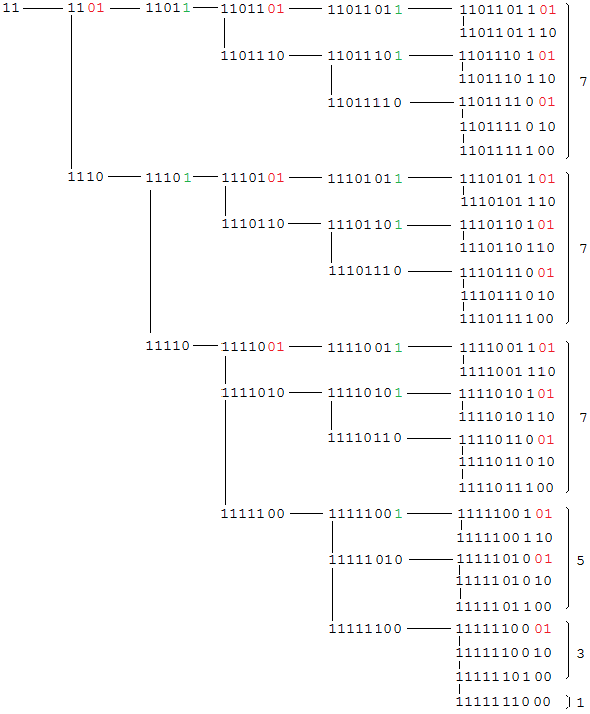
Figure 5: Directed rooted tree structure for the parity vectors up to $\mathbb{V}(6)$.

9.6 Parity vector set $\mathbb{V}(6)$ with integer solution $(x,y)$, $p$ and $h$

$\mathbb{V}(6)$

           $p$      parity vector        $(x,y)$      $h$

⬇

1 (1, 1, 0, 1, 1, 0, 1, 1, 0, 1) (1019, 545) 2

2 (1, 1, 0, 1, 1, 0, 1, 1, 1, 0) (1787, 955) 2

3 (1, 1, 0, 1, 1, 1, 0, 1, 0, 1) (2907, 1553) 2

4 (1, 1, 0, 1, 1, 1, 0, 1, 1, 0) (3675, 1963) 2

5 (1, 1, 0, 1, 1, 1, 1, 0, 0, 1) (1435, 767) 2

6 (1, 1, 0, 1, 1, 1, 1, 0, 1, 0) (2203, 1177) 2

7 (1, 1, 0, 1, 1, 1, 1, 1, 0, 0) (2587, 1382) 2

1 (1, 1, 1, 0, 1, 0, 1, 1, 0, 1) (3143, 1679) 3

2 (1, 1, 1, 0, 1, 0, 1, 1, 1, 0) (3911, 2089) 3

3 (1, 1, 1, 0, 1, 1, 0, 1, 0, 1) ( 935, 500) 3

4 (1, 1, 1, 0, 1, 1, 0, 1, 1, 0) (1703, 910) 3

5 (1, 1, 1, 0, 1, 1, 1, 0, 0, 1) (3559, 1901) 3

6 (1, 1, 1, 0, 1, 1, 1, 0, 1, 0) ( 231, 124) 3

7 (1, 1, 1, 0, 1, 1, 1, 1, 0, 0) ( 615, 329) 3

1 (1, 1, 1, 1, 0, 0, 1, 1, 0, 1) ( 463, 248) 4

2 (1, 1, 1, 1, 0, 0, 1, 1, 1, 0) (1231, 658) 4

3 (1, 1, 1, 1, 0, 1, 0, 1, 0, 1) (2351, 1256) 4

4 (1, 1, 1, 1, 0, 1, 0, 1, 1, 0) (3119, 1666) 4

5 (1, 1, 1, 1, 0, 1, 1, 0, 0, 1) ( 879, 470) 4

6 (1, 1, 1, 1, 0, 1, 1, 0, 1, 0) (1647, 880) 4

7 (1, 1, 1, 1, 0, 1, 1, 1, 0, 0) (2031, 1085) 4

1 (1, 1, 1, 1, 1, 0, 0, 1, 0, 1) (3295, 1760) 5

2 (1, 1, 1, 1, 1, 0, 0, 1, 1, 0) (4063, 2170) 5

3 (1, 1, 1, 1, 1, 0, 1, 0, 0, 1) (1823, 974) 5

4 (1, 1, 1, 1, 1, 0, 1, 0, 1, 0) (2591, 1384) 5

5 (1, 1, 1, 1, 1, 0, 1, 1, 0, 0) (2975, 1589) 5

1 (1, 1, 1, 1, 1, 1, 0, 0, 0, 1) (1087, 581) 6

2 (1, 1, 1, 1, 1, 1, 0, 0, 1, 0) (1855, 991) 6

3 (1, 1, 1, 1, 1, 1, 0, 1, 0, 0) (2239, 1196) 6

1 (1, 1, 1, 1, 1, 1, 1, 0, 0, 0) ( 383, 205) 7

In this example for $n=6$ it can be seen how the 30 parity vectors are ordered by their first 1-elements in direct progression. The number of these first 1-elements in each parity vector is equal to $h$. The listed order of the parity vectors is the exact order as the algorithm of Theorem 5 is generating the parity vectors, based on its tree structure. (cf. Figure 5)

10 Miscellaneous

All PARI/GP programs, tables and figures are written/created by the author.

This paper is dedicated to my high school mathematics teacher Dr. Franz Hagen.

Mike Winkler

Ernst-Abbe-Weg 4

45657 Recklinghausen, Germany

www.mikewinkler.co.nf

mike.winkler@gmx.de

11 References

References

- [1] David Applegate and Jeffrey C. Lagarias, Lower bounds for the total stopping time of 3x + 1 iterates, Mathematics of Computation, Vol. 72, No. 242 (June, 2002), pp. 1035 – 1049.
-
[2]
Lynn E. Garner, On the Collatz 3n + 1 Algorithm, Proc. Amer. Math. Soc., Vol. 82, No. 1 (May, 1981), pp. 19 – 22.
(http://www.jstor.org/stable/2044308) -
[3]
Jeffrey C. Lagarias, The 3x + 1 problem and its Generalizations, The American Mathematical Monthly Vol. 92, No. 1 (January, 1985), pp. 3 – 23.
(http://www.cecm.sfu.ca/organics/papers/lagarias/paper/html/paper.html) -
[4]
Matroids Matheplanet, Zahlentheorie-Forum, Beiträge 311 – 313.
(http://www.matheplanet.de/matheplanet/nuke/html/viewtopic.php?topic=222882) -
[5]
The On-Line Encyclopedia of Integer Sequences (OEIS), A020914, A020915, A022921, A056576, A076227, A100982, A177789, A293308
(http://oeis.org) -
[6]
The PARI Group - PARI/GP Version 2.9.0
(http://pari.math.u-bordeaux.fr) -
[7]
Eric Roosendaal, On the 3x + 1 problem, web document.
(http://www.ericr.nl/wondrous/terras.html) -
[8]
Riho Terras, A stopping time problem on the positive integers, Acta Arithmetica 30 (1976), 241–252.
(http://matwbn.icm.edu.pl/ksiazki/aa/aa30/aa3034.pdf) -
[9]
Wikipedia, Collatz conjecture
(https://en.wikipedia.org/wiki/Collatz_conjecture) -
[10]
Mike Winkler, New results on the stopping time behaviour of the Collatz 3x + 1 function, March 2015.
(http://arxiv.org/pdf/1504.00212v1.pdf) -
[11]
Mike Winkler, On a stopping time algorithm of the 3n + 1 function, May 2011.
(http://mikewinkler.co.nf/collatz_algorithm.pdf) -
[12]
Mike Winkler, On the structure and the behaviour of Collatz 3n + 1 sequences - Finite subsequences and the role of the Fibonacci sequence, November 2014.
(http://arxiv.org/pdf/1412.0519v1.pdf) -
[13]
Mike Winkler, Über das Stoppzeit-Verhalten der Collatz-Iteration, October 2010.
(http://mikewinkler.co.nf/collatz_algorithm_2010.pdf) -
[14]
Mike Winkler, Über die Struktur und das Wachstumsverhalten von Collatz 3n + 1 Folgen, March 2014.
(http://mikewinkler.co.nf/collatz_teilfolgen_2014.pdf)