Self-propulsion against a moving membrane: enhanced accumulation and drag force

Abstract

Self-propulsion (SP) is a main feature of active particles (AP), such as bacteria or biological micromotors, distinguishing them from passive colloids. A renowned consequence of SP is accumulation at static interfaces, even in the absence of hydrodynamic interactions. Here we address the role of SP in the interaction between AP and a moving semipermeable membrane. In particular, we implement a model of noninteracting AP in a channel crossed by a partially penetrable wall, moving at a constant velocity $c$. With respect to both the cases of passive colloids with $c>0$ and AP with $c=0$, the AP with finite $c$ show enhancement of accumulation in front of the obstacle and experience a largely increased drag force. This effect is understood in terms of an effective potential localised at the interface between particles and membrane, of height proportional to $c\tau/\xi$, where $\tau$ is the AP’s re-orientation time and $\xi$ the width characterising the surface’s smoothness ($\xi\to 0$ for hard core obstacles). An approximate analytical scheme is able to reproduce the observed density profiles and the measured drag force, in very good agreement with numerical simulations. The effects discussed here can be exploited for automatic selection and filtering of AP with desired parameters.

I Introduction

Active particles (AP) represent a large class of systems characterized by a conversion of internal energy into self-propulsion Ramaswamy (2010). The behavior of AP deeply differs from that of passive colloids in a thermal bath and shows typical features of nonequilibrium dynamics Cates (2012); Marconi et al. (2017). At the level of single trajectories, AP are characterized by persistent random walks and correlated motion. Instances of such systems can be found in the realm of bacteria and micro-organisms Marchetti et al. (2013), or in the context of man-made nano-devices Bechinger et al. (2016).

Several models have been proposed to study the physical properties of active matter systems, which show intriguing phenomena, such as nonequilibrium phase transitions, self-organization and collective behaviors. Let us mention the “run and tumble” model Tailleur and Cates (2008), characterized by directed motion interrupted by random reorientations, the “active Brownian” model Golestanian (2009); Palacci et al. (2010), where particles are pushed by a constant force, whose direction changes stochastically, and the Vicsek model Vicsek et al. (1995); Chaté et al. (2008), where the particle speed is fixed and the orientation depends on the average velocity of the neighbors. More recently, the Gaussian colored-noise (GCN) model has been proposed to account for the correlated motion (over a typical time $\tau$) characterizing AP systems Maggi et al. (2015), which allows for an analytical treatment within a specific scheme, known as Unified Colored Noise Approximation (UCNA) Jung and Hänggi (1987).

Among the several nonequilibrium phenomena observed in AP systems, a surprising result reproduced also by the GCN model, is that, in the presence of a static repulsive potential, AP do accumulate around the obstacle, producing a nontrivial density profile Wensink and Löwen (2008); Geiseler et al. (2016). This observation raises the question of what effects are produced when the obstacle is not static and moves with constant velocity, inducing a stationary current.

The study of the density profiles in (passive) colloidal systems under the action of a moving obstacle, indeed, takes on great importance in several contexts and has been addressed from different perspectives. For instance, it is the central issue in active microrheology, where a tracer is (magnetically or optically) driven through a medium to probe its structural properties Squires and Mason (2009); Puertas and Voigtmann (2014). A moving potential barrier can also be realized by means of optical fields, with travelling waves or inverted traps Volpe et al. (2014); Bianchi et al. (2016); Juniper et al. (2016). Moreover, soft potential barriers with a finite height and width are also used to model the finite thickness of a semipermeable membrane in contact with fluids Bryk (2006); Marsh et al. (1995); Margaritis and Rickayzen (1997); Zwanzig (1992), or the translocation properties of polymer chains through nanopores Sung and Park (1996); Ammenti et al. (2009). Similar problems related to the study of the stationary currents and density profiles of colloids under the effect of moving potentials have been addressed with the formalism of the density functional theory, with applications to the motion of colloidal particles in narrow channels Penna and Tarazona (2003a), or in polymer solutions Penna et al. (2003a); Tarazona and Marconi (2008).

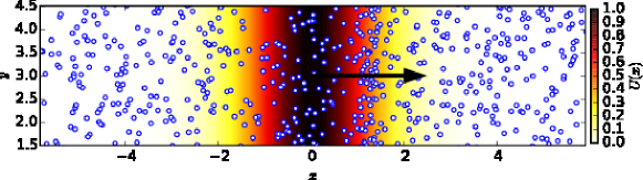
Figure 1: A semipermeable membrane, modeled as a potential barrier $U(x)$ (color-bar), moves at velocity $c$ (denoted by the arrow) in a fluid of noninteracting active particles.

In this paper, we study a simple model for a semipermeable membrane moving at constant velocity $c$ in a fluid of noninteracting GCN active particles of persistence time $\tau$, see the sketch in Fig. 1. Our analytical theory demonstrates the appearance of an effective dynamical potential arising from the coupling of self-propulsion with the nonequilibrium current induced by the moving obstacle: indeed it vanishes in both the limits of $c\to 0$, and $\tau\to 0$ (passive colloids with thermal noise). Our approach, which generalizes the UCNA to non-vanishing steady currents, gives accurate predictions - when compared to numerical simulations - for the density profiles of AP and the effective drag force, in a wide range of parameters. The most striking consequence of the current-induced effective potential is an enhanced accumulation of AP at the interface, with respect to the static case or with respect to the behavior of passive colloids. This effect yields a drag force whose intensity can be made large at will by tuning the model parameters. In the nonlinear regime of large $c$, we also observe a nonmonotonic behavior of the experienced drag force Leitmann and Franosch (2013); Bénichou et al. (2014, 2016), which is well described within our analytical approach. Our results have practical applications, e.g. in sweeping up AP from a mixture of inert/active particles, or in selecting and filtering AP with specific parameters, by tuning the properties of the moving membrane.

II Model

A channel, in generic dimension, contains suspended (active or passive) particles. A membrane separates the channel in two parts and moves with constant velocity $c$ along the direction $x$ perpendicular to itself, see Fig. 1. Since the particles are noninteracting, the only relevant direction is that parallel to the membrane movement. We assume the channel to be periodic and very large in the $x$ direction. The dynamics of each particle is described by the overdamped Langevin equation

$$\dot{x}(t) =\frac{F(x-ct)}{\zeta}+\eta(t),$$ (1)

$$F(x) =-d_{x}U(x),$$ (2)

where the potential $U(x)$ represents the moving penetrable membrane. The width of the membrane is used as unit of length (see below, Eq. (5)), while the mass of the particle is 1. The quantity $\eta(t)$ stands for a noise term, which is white (thermal) for passive colloids, or coloured, with correlation time $\tau$, for active particles: in both cases $\langle\eta(t)\rangle=0$. When Eq. (1) models passive particles, we take $\langle\eta(t)\eta(t^{\prime})\rangle=\frac{2}{\zeta}\delta(t-t^{\prime})$ and the host fluid has unitary temperature: therefore $\zeta$ is the viscosity of the host fluid in these particular units. When Eq. (1) models active particles, $\eta(t)$ is GCN (“active noise”), i.e.

$$\dot{\eta}(t) =-\zeta\eta(t)+\sqrt{2\zeta}\chi(t)$$ (3)

$$\langle\chi(t)\chi(t^{\prime})\rangle =\delta(t-t^{\prime}).$$ (4)

In this case $\zeta=1/\tau$ and the active effective temperature is set to $1$ (or, equivalently, the active speed is set to $1$). We notice that in both cases (passive and active), with chosen units, the bare diffusion coefficient of the particles (i.e. when $U(x)\equiv 0$) is $1/\zeta$. In the following, we use a smooth potential of the form

$$U(x)=U_{0}\{\tanh[(x+1)/\xi]-\tanh[(x-1)/\xi]\},$$ (5)

which is characterised by a steepness $1/\xi$.

In order to understand the main effects induced by self-propulsion in the presence of a stationary current, we focus on two quantities: i) the density profile around the moving obstacle and ii) the experienced drag force.

II.1 Effective potential

To proceed with our analysis, it is useful to notice that, when $\eta(t)$ is GCN, we can time-derive Eq. (1), obtaining

$$\dot{x}(t) =v(t),$$ (6)

$$\dot{v}(t) =-\zeta g(x-ct)v(t)+F^{*}(x-ct)+\sqrt{2\zeta}\chi(t),$$ (7)

$$F^{*}(x) =F(x)-\frac{c}{\zeta}\frac{dF(x)}{dx}=-\frac{dU(x)}{dx}+\frac{c}{\zeta}\frac{d^{2}U(x)}{dx^{2}},$$ (8)

$$g(x)= 1+\frac{1}{\zeta^{2}}\frac{d^{2}U(x)}{dx^{2}}.$$ (9)

In the above equations two terms deserve discussion: an effective force $F^{*}(x)$, which reduces to $-dU/dx$ when $c=0$, and an effective viscosity $g(x)$. The latter - which is the only effect of self-propulsion when $c=0$ - has been thoroughly discussed in Maggi et al. (2015); Marconi and Maggi (2015); Marconi et al. (2016): it can be treated within an approximate equilibrium-like solution (known as UCNA), based upon an effective static potential $U_{stat}(x)=U(x)+\frac{1}{2\zeta^{2}}\left(\frac{dU(x)}{dx}\right)^{2}-\ln|g(x)|$. In the present case, the finite velocity of the obstacle $c>0$ produces an additional contribution in the force term, which is responsible for new dynamical effects. These effects can be accounted for by a new approximate treatment (see Appendix A).

III Dynamical UCNA

In the case of a shifting barrier, one rewrites the stochastic differential equations (6)-(7) into the equivalent Fokker-Planck equation for the probability distribution of position and velocity $P(y,v)$:

$$\frac{\partial P(y,v)}{\partial t}+v\frac{\partial}{\partial y}P(y,v)+F^{*}(y)\frac{\partial}{\partial v}P(y,v)$$

$$=\zeta\frac{\partial}{\partial v}\Bigl{[}\frac{\partial}{\partial v}+g(y)v\Bigl{]}P(y,v),$$ (10)

with $y=x-ct$. In order to proceed further, we consider the steady state solution of Eq. (10) and set $\frac{\partial P(y,v)}{\partial t}=-c\frac{\partial P(y,v)}{\partial y}$. By multiplying by powers of $v$ and integrating w.r.t. $v$, one obtains a hierarchy of coupled first order ordinary differential equations for the velocity moments of $P(y,v)$, whose first two members are the continuity equation for the density $\rho(y)=\int dvP(y,v)$

$$-c\frac{d\rho(y)}{dy}+\frac{d}{dy}J(y)=0,$$ (11)

and the momentum balance equation for the current $J(y)=\int dvvP(y,v)$:

$$-c\frac{dJ(y)}{dy}+\frac{d\Pi(y)}{dy}-F^{*}(y)\rho(y)-\zeta g(y)J(y)=0,$$ (12)

where $\Pi(y)=\int dvv^{2}P(y,v)$. According to Eq. (11) the current must be proportional to the density

$$J(y)=c[\rho(y)-\bar{\rho}],$$ (13)

where $\bar{\rho}$ is a constant such that the solution is periodic, $\rho(L)=\rho(-L)$. The following distribution represents the exact solution of Eq. (10) in the regions where the force vanishes and contains adjustable parameters to obtain an approximate solution in the wall region:

$$P(y,v) = \sqrt{\frac{\beta(y)}{2\pi}}\left\{[\rho(y)-\bar{\rho}]\exp\left[-\frac{1}{2}\beta(y)(v-c)^{2}\right]\right.$$ (14)

$$+ \left.\bar{\rho}\exp\left[-\frac{1}{2}\beta(y)v^{2}\right]\right\},$$

where $\beta(y)$ is a positive definite function. Remarkably, expression (14) also represents an (approximate) closure of the infinite hierarchy of equations (of which Eqs. (11) and (12) are the first two members) generated by the transformation of the partial differential equation  (10) into a set of coupled ordinary differential equations for the velocity moments of $P$. Hence, according to the information contained in Eq. (14) the momentum flux reads $\Pi(y)=\frac{\rho(y)}{\beta(y)}+c^{2}[\rho(y)-\bar{\rho}]$, so that Eq. (12) becomes:

$$\frac{d}{dy}\frac{\rho(y)}{\beta(y)}=[F(y)-\zeta c]\rho(y)+\zeta cg(y)\bar{\rho},$$ (15)

which has the following interpretation: the “active pressure” gradient $\frac{d}{dy}\frac{\rho(y)}{\beta(y)}$ is balanced by the force due to the moving wall and by the friction force $-\zeta g(y)J(y)$ (the second term in the r.h.s.). In the case of a very weak potential, $\rho(y)\approx\bar{\rho}$ and the current vanishes, whereas for high barriers $\rho(y)\gg\bar{\rho}$ and $J(y)\approx c\rho(y)$. The static UCNA approximation is recovered by setting $c=0$, i.e. $J=0$ and $\beta(y)=g(y)$. The density profile is given by:

$$\frac{\rho(y)}{\beta(y)} = \frac{\rho(L)}{\beta(L)}e^{-w(y)+w(-L)-c\zeta(y+L)}$$ (16)

$$+ \zeta c\bar{\rho}e^{-w(y)-\zeta cy}\int_{-L}^{y}dse^{w(s)+c\zeta s}g(s),$$

where $w(y)$ is an effective potential defined by:

$$w(y)=\int_{-L}^{y}ds\beta(s)\frac{dU(s)}{ds}+\zeta c\int_{-L}^{y}ds[\beta(s)-1],$$ (17)

and $\rho(L)$ is fixed by the normalization of the number of particles. The explicit expression of the constant $\bar{\rho}$ is given in Appendix A. Interestingly, the second term in the r.h.s. of Eq. (17) can be identified with a dynamical potential $U_{dyn}(y)$ vanishing when either $c=0$ (static barrier) or $\zeta\to\infty$ (passive particles). Therefore it is a peculiar feature of our model, arising from the coupling of self-propulsion with the nonequilibrium current. This term gives an effective trap – at the front of the moving potential – of height $\sim U_{0}c/(\zeta\xi)$, and a specular effective barrier at its tail. As one can see, the solution for $c\neq 0$ is not Boltzmann-like since the system is in a truly nonequilibrium state and therefore the density profile is not symmetric with respect to the transformation $y\to-y$ which characterizes the bare potential $U(y)$.

Since the UCNA breaks down in regions with negative curvature of the potential Jung and Hänggi (1987), for the purpose of obtaining quantitative predictions for $\rho(y)$, we empirically set $\beta(y)=g(y)$ where $g(x)\geq 0$, and $\beta(y)=0$ otherwise. From the density profile $\rho(y)$ we also obtain the average drag force acting on the moving barrier $\langle F\rangle=\int_{-L}^{L}dyF(y)\rho(y)$, which obeys the sum rule

$$\langle F\rangle=\zeta c\int_{-L}^{L}dy[\rho(y)-g(y)\bar{\rho}].$$ (18)

IV Numerical results

The approximations underlying our theory have been fairly verified by comparison with numerical simulations of the model in Eq. (1), for both passive and active particles. The simulations implement a time-discretized scheme for Eq. (1) through a fourth-order Runge-Kutta algorithm Honeycutt (1992), with a time step $dt=10^{-4}$. Averages are done on a single trajectory of length $5\times 10^{8}$ in the used units. In the figures, error bars fall within the symbols.

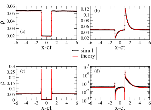
Figure 2: Density profiles with different kinds of noise (thermal or active) and different values of the barrier’s velocity $c$: (a) thermal noise, $c=0$: (b) thermal noise, $c=0.2$; (c) active noise, $c=0$; (d) active noise, $c=0.2$.

In Fig. 2 we show the density profiles for two passive cases and two active cases, with static or moving potential. A first important information is the good match between simulations and theory. In the passive case (two top frames), switching on the external velocity from $c=0$ to $c>0$ leads to an imbalance of the density distribution with an accumulation at the front of the membrane (at $x-ct=1$, see expression of the moving potential, Eq. (5)), and a depletion at its tail (at $x-ct=-1$) . The two frames on the left ($c=0$) demonstrate that switching from passive to active particles induces an accumulation of particles near both borders of the membrane potential, with a depletion inside the energetically unfavoured region. The novel effect discussed here appears, strikingly, in the active case with $c>0$ (bottom-right frame): the accumulation of particles on the moving front of the membrane becomes much more important than the passive case with $c>0$ or the active case with $c=0$ (notice the log scale on the $y$ axis).

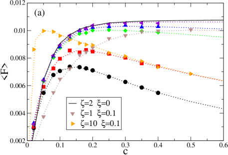
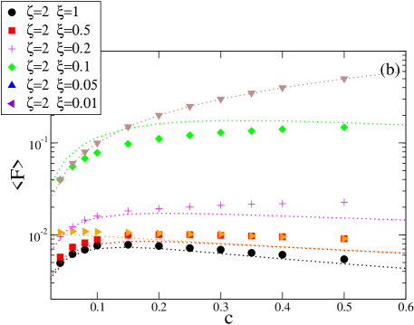
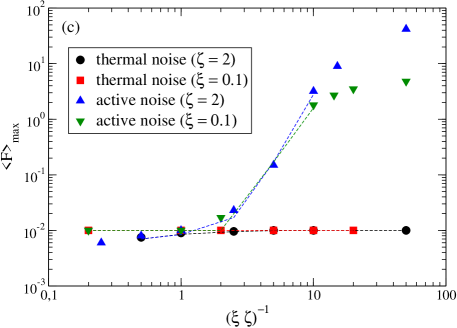
Figure 3: (a) and (b): average drag force versus velocity $c$ for thermal noise (a) and active noise (b). Symbols represent numerical simulations (legends are valid for both graphs), while dotted lines are the theoretical predictions; (c): maximum average drag force versus $(\xi\zeta)^{-1}$. Symbols are numerical simulations, while lines are from theory.

To understand the behavior of the system in full generality, exploring the effects of all parameters, we focus on the global observable $\langle F(y)\rangle$, which is the average drag force experienced by the moving membrane. Several results are shown in Fig. 3A and 3B, where a comparison is presented between passive and active cases for several values of $\zeta$ and $\xi$ in a relevant range of velocities $c$. Again, we observe a fair superposition of numerical results with theoretical predictions, Eq. (18): this is expected for the passive cases, where the theory is exact, while it is not trivial at all in the active case. Surprisingly, even at low $\xi$, a reduction of $\zeta$ (longer activity persistence time $\tau$) may improve the agreement with the simulations.

In all the cases considered (excluding the $\xi\to 0$ limit for the passive case), at constant $\xi$ and $\zeta$, the average drag reaches a maximum at some value $c^{*}$ and then decreases for $c>c^{*}$. This can be understood in terms of competition between “kinetic energy” $\sim c^{2}$ and the potential barrier. In the passive case this leads to a value of $c^{*}$ which is roughly independent of $\xi$ or $\zeta$, and a saturation of $\langle F\rangle$ when $\xi\to 0$, as seen in Fig. 3A. In the active case at large $1/(\xi\zeta)$ the dynamic potential $\sim U_{0}c/(\zeta\xi)$ dominates, so that the energetic argument leads to $c^{*}\sim U_{0}/(\zeta\xi)$. When the effective barrier is high and $c<c^{*}$, very few particles cross it and the majority goes at $\dot{x}\sim c$, so that Eq. (1) on average gives the linear behavior $\langle F\rangle\approx\zeta c$, well visible in simulations at large values of $1/(\zeta\xi)$. Estimating the maximum value of the drag force to be $\langle F\rangle_{max}\approx\zeta c^{*}$, we get for the active case $\langle F\rangle_{max}\approx U_{0}/\xi$, expected to hold at large $(\zeta\xi)^{-1}$. The active case with a moving membrane, therefore, is qualitatively different from the passive case - or from any case at $c=0$ - since the average drag force can increase indefinitely by reducing $\xi$. In Fig. 3C we have shown $\langle F\rangle_{max}$ versus $(\zeta\xi)^{-1}$ for the active and passive cases: at intermediate values of $(\zeta\xi)^{-1}$ an interesting data collapse is found, together with a sharp increase with $(\zeta\xi)^{-1}$ for the active case. Such an increase eventually saturates if $\zeta$ is further decreased at constant $\xi$, or continues if $\xi$ is reduced at constant $\zeta$, demonstrating the qualitative difference between the active and the passive cases.

V Conclusions

We have shown the existence of a dynamical enhancement of clustering and drag when a travelling barrier sweeps active particles. The synergy of two dynamical effects (active noise and non-zero current) leads to a scenario qualitatively new, as shown in Fig. 3C: indeed the average drag is sensitive to the persistence time $1/\zeta$ and to the steepness of the membrane potential $1/\xi$, and can be made indefinitely strong. We have discussed a theoretical treatment of this effect, fairly compared with numerical simulations. This is remarkable if one considers that predictive theoretical schemes are scarce in the framework of active particles, particularly in the non-linear regime with strong spatial currents as in our case. It is interesting to note that our theory truncates the Fokker-Planck hierarchy at the same order of the static UCNA scheme: however, unlike the static UCNA, it leads to a genuine non-equilibrium behavior Fodor et al. (2016); Marconi et al. (2017).

The parameter values used in our simulations are in the range of realistic systems of AP, therefore they are within reach for experimental verification, e.g. in setups with optical travelling waves or inverted traps Volpe et al. (2014); Bianchi et al. (2016); Juniper et al. (2016), taking care to avoid competing effects such as diffusiophoretic torques or hydrodynamic-induced wall-attachment Wysocki et al. (2015); Lozano et al. (2016). For instance, taking as unit of length $10\mu m$ (order of magnitude of the width of lithographed micro-membrane), typical biological swimmers with speed $\sim 10\mu m/s$ and reorientation time $\tau\sim 1s$ correspond to $\zeta\approx 1$. A straightforward application of our study is the possibility to separate a mixture of AP, filtering out those with given parameters (e.g. a certain value of $\tau$) by sweeping a membrane with well-tuned values of $c$ and $\xi$.

Appendix A Model equations

We consider a dilute solution of active particles dragged along the x-direction under the action of a travelling potential barrier with velocity $c$, modelled by a time dependent external potential, $U(x,t)=U(x-ct)$, which acts on the colloidal particles but has negligible effects on the solvent Penna and Tarazona (2003b); Penna et al. (2003b); Tarazona and Marini Bettolo Marconi (2008). For the sake of simplicity we neglect the interactions among the particles and any hydrodynamic effect and include only the friction, through a drag coefficien $\gamma$. The active forces are modelled by a coloured noise, i.e. Gaussian noise with exponential memory of characteristic time $\tau$. Note that, in this Appendix, we introduce the model with all dimensional parameters and explicitly show the change of variables necessary to obtain the Equations studied in the paper.

A.0.1 Langevin description

The following stochastic dynamics is assumed

$$\dot{x}(t)=\frac{1}{\gamma}F(x,t)+\eta(t)\,,$$ (19)

where $F=-\partial U/\partial x$ and $\eta$ mimics the self-propulsion mechanism and is assimilated to an Ornstein-Uhlenbeck process

$$\dot{\eta}(t)=-\frac{1}{\tau}\eta(t)+\frac{D^{1/2}}{\tau}\xi(t).$$ (20)

The underlying stochastic force $\xi(t)$ is a Gaussian and Markovian process distributed with zero mean and moments $\langle\xi(t)\xi(t^{\prime})\rangle=2\delta(t-t^{\prime})$. The coefficient $D$ due to the activity is related to the correlation of the Ornstein-Uhlenbeck process $\eta(t)$ via

$$\langle\eta(t)\eta(t^{\prime})\rangle=\frac{D}{\tau}\exp\Bigl{(}-\frac{|t-t^{\prime}|}{\tau}\Bigr{)}.$$ (21)

A.0.2 Fokker-Planck description

After differentiating with respect to time eq. (19) and introducing a velocity $v=\dot{x}$, we may write the following system of equations:

$$\dot{x} = v$$

$$\dot{v} = -\frac{1}{\tau}\left(1-\frac{\tau}{\gamma}\frac{\partial F}{\partial x}\right)v+\frac{1}{\tau\gamma}\Bigl{(}F+\tau\frac{\partial F}{\partial t}\Bigr{)}+\frac{D^{1/2}}{\tau}\eta\,.$$ (22)

The latter equation in the case of the shifting potential becomes:

$$\dot{v}=-\frac{1}{\tau}\left(1-\frac{\tau}{\gamma}\frac{\partial F}{\partial x}\right)v+\frac{1}{\tau\gamma}\Bigl{(}F-\tau c\frac{\partial F}{\partial x}\Bigr{)}+\frac{D^{1/2}}{\tau}\eta$$ (23)

and the associated Fokker-Planck (FP) equation for the ”phase-space” distribution $P(x,v,t)$ reads

$$\frac{\partial P}{\partial t}+v\frac{\partial P}{\partial x}+\Bigl{(}\frac{F(x,t)+\tau\frac{\partial F(x,t)}{\partial t}}{\gamma\tau}\Bigr{)}\frac{\partial P}{\partial v}=\frac{1}{\tau}\frac{\partial}{\partial v}\Bigl{(}\frac{D}{\tau}\frac{\partial}{\partial v}+g(x,t)v\Bigl{)}P\,,$$ (24)

where $g(x,t)=\left(1-\frac{\tau}{\gamma}\frac{\partial F}{\partial x}\right)$.

Now, defining $F^{*}=(F-\tau c\frac{\partial F}{\partial x})$ and considering the steady state regime of the system, where $P(x,v,t)$ must have the travelling wave form $P(x-ct,v)$, we can write:

$$-c\frac{\partial P}{\partial x}+v\frac{\partial P}{\partial x}+\frac{F^{*}(x-ct)}{\gamma\tau}\frac{\partial P}{\partial v}=\frac{1}{\tau}\frac{\partial}{\partial v}\Bigl{(}\frac{D}{\tau}\frac{\partial}{\partial v}+g(x-ct)v\Bigl{)}P.$$ (25)

In the problem at hand, the shifting external potential $U$ is localized within a finite region around the origin of the comoving reference frame and vanishes for $x\to\pm\infty$.

A.0.3 Non dimensional variables

In order to proceed further, it is time saving to adopt non dimensional variables for positions, velocities, and time, and rescale forces accordingly. We define $v_{T}=\sqrt{D/\tau}$, measure lenghts using the characteristic lenght, $\ell$, of the potential and introduce the following non dimensional variables:

$$\bar{t}\equiv t\frac{v_{T}}{l},\qquad\bar{v}\equiv\frac{v}{v_{T}},\qquad X\equiv\frac{x}{\ell},\qquad\bar{F}(\bar{x},\bar{t})\equiv\frac{\ell F(x,t)}{D\gamma},\qquad\zeta=\frac{\ell}{\tau v_{T}},\qquad\bar{P}=v_{T}\ell\,P,\qquad\bar{c}=\frac{c}{v_{T}},$$ (26)

where $\zeta$ plays the role of a non dimensional friction. To lighten the notation we shall drop the bar over the non dimensional variables without incurring in ambiguities.

In the case of a shifting barrier, one can write the following Fokker-Planck equation in terms of the coordinate $y=x-ct$ relative to the comoving reference frame:

$$-c\frac{\partial P(y,v)}{\partial y}+v\frac{\partial}{\partial y}P(y,v)+F^{*}(y)\frac{\partial}{\partial v}P(y,v)=\zeta\frac{\partial}{\partial v}\Bigl{[}\frac{\partial}{\partial v}+g(y)v\Bigl{]}P(y,v)\,$$ (27)

A.0.4 Hydrodynamic theory

In order to proceed further, it is convenient to eliminate the $v$ dependence of the phase-space distribution $P(y,v)$, by multiplying by powers of $v$ and integrating w.r.t. $v$. One obtains a set of coupled first order ordinary differential equations, the so-called Brinkman hierarchy, whose first two members are the continuity equation and the momentum balance equation, respectively:

$$-c\frac{d\rho(y)}{dy}+\frac{d}{dy}J(y)=0\,,$$ (28)

$$-c\frac{dJ(y)}{dy}+\frac{d\Pi(y)}{dy}-F^{*}(y)\rho(y)+\zeta g(y)J(y)=0$$ (29)

where we have introduced the density $\rho(y)$, the current $J(y)$ and the momentum current $\Pi(y)$, respectively, via:

$$\rho(y) = \int dvP(y,v)\,,$$ (30)

$$J(y) = \int dvvP(y,v)\,,$$ (31)

$$\Pi(y) = \int dvv^{2}P(y,v)\,.$$ (32)

According to the continuity equation (28) the current must be proportional to the density

$$J(y)=c[\rho(y)-\bar{\rho}]\,,$$ (33)

where $\bar{\rho}$ is a constant such that the solution is periodic at $\rho(L)=\rho(-L)$, where $2L$ is the box size. As we shall see later, for large systems $L\gg\ell$, $\bar{\rho}\approx\rho(\pm L)$ and the current is almost vanishing at the boundaries.

It can be easily verified that the following distribution is a solution of the eq. (27) in regions where $F^{*}(y)=0$ and $g(y)=1$:

$$P(y,v)=\Bigl{[}\rho(y)-\bar{\rho}\Bigr{]}\,H_{0}(v-c)+\bar{\rho}\,H_{0}(v)\,,$$ (34)

where

$$H_{0}(v)=\frac{1}{\sqrt{2\pi}}\exp\Bigl{(}-\frac{1}{2}v^{2}\Bigr{)}$$ (35)

is a Hermite function of zeroth order. By substituting the ansatz (34) in eq. (27) (with $F=0$) we obtain a solution provided $\rho(y)$ satisfies the following condition:

$$\frac{d\rho(y)}{dy}=-\zeta c(\rho(y)-\bar{\rho})\,.$$ (36)

A.0.5 Solution in the presence of a force field

Now, we insist in looking for a solution of eq.  (27) of the form:

$$P(y,v)=\Bigl{[}\rho(y)-\bar{\rho}\Bigr{]}\,H_{0}(y,v-c)+\bar{\rho}\,H_{0}(y,v)\,,$$ (37)

even in the region where $F(y)\neq 0$. We have introduced the following (non uniform) Hermite functions, which are position dependent through $\beta(y)$, an adjustable function:

$$H_{0}(y,v) = \sqrt{\frac{\beta(y)}{2\pi}}\exp\Bigl{(}-\frac{\beta(y)}{2}v^{2}\Bigr{)}\,,$$ (38)

$$H_{1}(y,v) = \sqrt{\frac{\beta(y)}{2\pi}}\beta^{1/2}(y)\,v\,\exp\Bigl{(}-\frac{\beta(y)}{2}v^{2}\Bigr{)}\,.$$ (39)

If we do that, i.e. if we apply the full FP operator to the trial distribution (37) we get:

$$H_{1}(y,v-c)\frac{1}{\beta^{1/2}}\Bigl{(}\frac{d\rho(y)}{dy}-\beta(F^{*}-\zeta gc)(\rho-\bar{\rho})-\frac{\beta^{\prime}}{\beta}(\rho-\bar{\rho})\Bigr{)}-H_{1}(y,v))\frac{1}{\beta^{1/2}}\Bigl{(}\beta F^{*}\bar{\rho}+\frac{\beta^{\prime}}{\beta}\bar{\rho}\Bigr{)}$$

$$+\zeta(g-\beta)\Bigl{(}(\rho-\bar{\rho})H_{2}(y,v-c)+\bar{\rho}H_{2}(y,v)\Bigr{)}-\frac{\beta^{\prime}}{2\beta^{3/2}}\Bigl{(}(\rho-\bar{\rho})H_{3}(y,v-c)+\bar{\rho}H_{3}(y,v)-c\beta^{1/2}H_{2}(y,v)\Bigr{)}=0\,,$$

(40)

where $H_{2}(y,v)$ and $H_{3}(y,v)$ are the Hermite functions of order 2 and 3, respectively, and given by the recursion relation:

$$H_{\nu+1}(y,v)=-\frac{1}{\beta^{1/2}}\frac{\partial H_{\nu}(y,v)}{\partial v}.$$

The trial solution fails to solve eq.  (27). However, if we limit ourselves to consider only the two lowest moments of the probability distribution, i.e. if after multiplying by $(v-c)$, we integrate (40) over $v$ we obtain the following condition which gives the profile equation:

$$\frac{1}{\beta}\frac{d\rho(y)}{dy}-(F-\zeta c)\rho(y)-\frac{\beta^{\prime}}{\beta^{2}}\rho(y)-\zeta cg\bar{\rho}=0\,.$$ (41)

If we continue the projection procedure beyond the first order in $(v-c)$ there will be an error in the equation for the second moment, which becomes inconsistent with the value of the second moment imposed by the trial distribution (which, in fact, is already fixed by the trial form and therefore does not contain enough parameters to satisfy the extra conditions.).

A.0.6 Construction of the solution

Eq. (41) can be rearranged as follows:

$$\frac{d}{dy}\frac{\rho(y)}{\beta(y)}=(F(y)-\zeta c)\rho(y)+\zeta cg(y)\bar{\rho}.$$ (42)

Notice that the ansatz for the phase-space distribution, gives the following expression for the momentum flux:

$$\Pi(y)=\frac{\rho(y)}{\beta(y)}+c^{2}(\rho(y)-\bar{\rho})\,.$$ (43)

Notice that eq. (41) is perfectly equivalent to eq. (29) when the latter is endowed with a closure, indeed represented by eq. (43). The static UCNA approximation is recovered by setting the arbitrary function $\beta(y)=g(y)$ and $c=0$, (i.e. $J=0$). The solution of the inhomogeneous equation in the case of $c\neq 0$ is

$$\rho(y)=\frac{\rho(L)}{\beta(L)}\beta(y)e^{-(w(y)-w(-L))-c\zeta(y+L)}\Bigl{[}1+(e^{2\zeta cL}e^{w(L)-w(-L)}-1)\frac{\int_{-L}^{y}dse^{w(s)+c\zeta s}g(s)}{\int_{-L}^{L}dse^{w(s)+c\zeta s}g^{(}s)}\Bigr{]}\,,$$ (44)

where $\rho(L)$ is fixed by the normalization and the effective potential $w(y)$ is defined by

$$w(y)=\int_{-L}^{y}ds\beta(s)\frac{dU(s)}{ds}+\zeta c\int_{-L}^{y}ds[\beta(s)-1]\,,$$ (45)

The function $\beta(y)$ is given by $g(y)$ when $g(y)>0$ and $\beta(y)=0$ otherwise.

A.0.7 Average Force and sum rule

The average drag force is given by

$$<F>=\int_{-L}^{L}dyF(y)\rho(y)=\zeta c\int_{-L}^{L}dy[\rho(y)-\bar{\rho}g(y)].$$ (46)

The constant $\bar{\rho}$ is

$$\bar{\rho}=\frac{1}{\zeta c}\frac{\rho(L)}{\beta(L)}\frac{\Bigl{(}e^{w(L)+c\zeta L}-e^{w(-L)-c\zeta L}\Bigr{)}}{\int_{-L}^{L}dye^{w(y)+c\zeta y}g(y)}$$

and we can rewrite the solution as:

$$\frac{\rho(y)}{\beta(y)}=\frac{\rho(L)}{\beta(L)}e^{-w(y)+w(-L)-c\zeta(y+L)}+\zeta c\bar{\rho}e^{-w(y)-\zeta cy}\int_{-L}^{y}dse^{w(s)+c\zeta s}g(s).$$ (47)

Finally, in order to regularize the problem we have chosen $\beta(y)=g(y)$ when $g(y)>0$ and $\beta(y)=0$ otherwise.

Appendix B The Dual picture

The same mathematical problem can describe a different physical set up. Consider a one dimensional system and a non uniform potential $U(y)$ acting in a central region only, where $F(y)=-\frac{dU}{dy}\neq 0$. The particles are subject to colored noise and to a uniform force $E$. There will be a constant current, say $J_{0}$.

The obstacle is fixed in space, represented by the force $F(y)$. There is a constant external field $E$

$$\dot{y}=\frac{F(y)+E}{\gamma}+\eta(t)$$ (48)

where $\eta(t)$ is the standard colored noise as before. Time-differentiating Eq. (48) we get

$$\dot{y}=v$$ (49)

$$\dot{v}=\frac{F^{\prime}(y)}{\gamma}v-\frac{v(t)}{\tau}+\frac{F+E}{\tau\gamma}+\frac{D^{1/2}}{\tau}\xi\,.$$ (50)

Equivalently, we write the associated FP equation:

$$\frac{\partial P}{\partial t}+v\frac{\partial P}{\partial y}+\Bigl{(}\frac{F(y)+E}{\gamma\tau}\Bigr{)}\frac{\partial P}{\partial v}=\frac{1}{\tau}\frac{\partial}{\partial v}\Bigl{(}\frac{D}{\tau}\frac{\partial}{\partial v}+g(y)v\Bigl{)}P\,,$$ (51)

which for a stationary system becomes

$$v\frac{\partial P}{\partial y}+\Bigl{(}\frac{F(y)+E}{\gamma\tau}\Bigr{)}\frac{\partial P}{\partial v}=\frac{1}{\tau}\frac{\partial}{\partial v}\Bigl{(}\frac{D}{\tau}\frac{\partial}{\partial v}+g(y)v\Bigl{)}P\,.$$ (52)

In non dimensional form we have:

$$v\frac{\partial}{\partial y}P(y,v)+(F(y)+E)\frac{\partial}{\partial v}P(y,v)=\zeta\frac{\partial}{\partial v}\Bigl{[}\frac{\partial}{\partial v}+g(y)v\Bigl{]}P(y,v)\,.$$ (53)

If one integrates over $v$ and defines $J(y)=\int dvvP(y,v)$, one finds:

$$\frac{d}{dy}J(y)=0\,.$$ (54)

The current is, now, constant: $J(y)=J_{0}$. Let us multiply by $v$ and integrate eq. (52):

$$\frac{d}{dy}\Pi(y)-(F(y)+E)\rho(y)=-\zeta g(y)J_{0}\,,$$ (55)

with $\Pi(y)=\int v^{2}P(y,v)dv$. Let us invert the relation and make the ansatz:

$$P(y,v)=\bar{\rho}H_{0}(y,v-u)+(\rho(y)-\bar{\rho})H_{0}(y,v)$$ (56)

Substituting (56) in eq. (53) when $F=0$ and $g=1$ we obtain

$$H_{1}(v)\Bigl{(}\frac{d\rho(y)}{dy}-E(\rho(y)-\bar{\rho})\Bigr{)}-\Bigl{(}E\bar{\rho}-\zeta c\bar{\rho}\Bigr{)}H_{1}(v-u)=0\,,$$ (57)

whose solution is:

$$\frac{d\rho(y)}{dy}-E(\rho(y)-\bar{\rho})=0$$ (58)

$$E\bar{\rho}=\zeta u\bar{\rho}$$ (59)

Now, we go back to eq. (55) and use the following closure (contained already in the parametric form of the solution for $P(y,v)$):

$$J(y) = J_{0}=\bar{\rho}u\,,$$ (60)

$$\Pi(y) = \bar{\rho}u^{2}+\frac{\rho(y)}{\beta(y)}\,.$$ (61)

So that the equation for $\rho(y)$ reads:

$$\frac{d}{dy}\frac{\rho(y)}{\beta(y)}-(F(y)+E)\rho(y)=-\zeta ug(y)\bar{\rho}\,.$$ (62)

Now, such an equation is identical to the equation (42) , provided we identify:

$$E = -\zeta c\,,$$ (63)

$$u = -c\,,$$ (64)

$$u = \frac{E}{\zeta}\,.$$ (65)

Thus, we have shown that the equation for $\rho(y)$ is of the same type as the Nernst-Planck (NP) equation: The NP equation assumes that the constant current $J_{0}$ results from the combined effects of a diffusive current due to the random fluctuations ( the ”thermal agitation” in other words) and a deterministic migration current due to the coupling to an external field $E$, which can be also modified by the presence of some localized potential $U=-\int^{y}F(s)ds$:

$$J_{0}=-\frac{1}{\zeta}\frac{1}{g(y)}\frac{d}{dy}\frac{\rho(y)}{\beta(y)}+\frac{1}{\zeta g(y)}(F(y)+E)\rho(y)\,,$$ (66)

with a space-dependent diffusion coefficient

$$D(y)\equiv\frac{1}{\zeta}\frac{1}{\beta(y)g(y)}$$ (67)

and a space-dependent mobility

$$\mu(y)=\frac{1}{\zeta}\frac{1}{g(y)}\,.$$ (68)

Notice that this is exactly the UCNA equation for the current, which can be derived without phase-space considerations.

Finally, let us rewrite

$$J_{0}=-\frac{d}{dy}\Bigl{(}D(y)\rho(y)\Bigr{)}+\mu(y)\Bigl{(}F(y)+E-\frac{1}{\beta(y)}\frac{d}{dy}\ln g(y)\Bigr{)}\rho(y)$$ (69)

There is an extra contribution from the drift stemming from the colored noise.

Note that the mathematics is the same as for the original problem, but the interpretation of each term is now different. If we look at the profiles, we observe a crowding of active particles at the front of the potential (where the derivative of $U$ is largest) and a depletion inside. Particle near the entrance loose mobility and therefore crowd there. With strong activity and sharp entrances ($\zeta\to 0$ and $\xi\to 0$, respectively) the current should go to zero.

References

- Ramaswamy (2010) S. Ramaswamy, Annu. Rev. Condens. Matter Phys. 1, 323 (2010).
- Cates (2012) M. Cates, Rep. Prog. Phys. 75, 042601 (2012).
- Marconi et al. (2017) U. M. B. Marconi, A. Puglisi, and C. Maggi, Sci. Rep. 7, 46496 (2017).
- Marchetti et al. (2013) M. C. Marchetti, J. F. Joanny, S. Ramaswamy, T. B. Liverpool, J. Prost, M. Rao, and R. A. Simha, Rev. Mod. Phys. 85, 1143 (2013).
- Bechinger et al. (2016) C. Bechinger, R. D. Leonardo, H. Löwen, C. Reichhardt, G. Volpe, and G. Volpe, Rev. Mod. Phys. 88, 045006 (2016).
- Tailleur and Cates (2008) J. Tailleur and M. E. Cates, Phys. Rev. Lett. 100, 218103 (2008).
- Golestanian (2009) R. Golestanian, Phys. Rev. Lett. 102, 188305 (2009).
- Palacci et al. (2010) J. Palacci, C. Cottin-Bizonne, C. Ybert, and L. Bocquet, Phys. Rev. Lett. 105, 088304 (2010).
- Vicsek et al. (1995) T. Vicsek, A. CzirÃŗk, E. Ben-Jacob, I. Cohen, and O. Shochet, Phys. Rev. Lett. 75, 1226 (1995).
- Chaté et al. (2008) H. Chaté, F. Ginelli, G. Grégoire, and F. Raynaud, Phys. Rev. E 77, 046113 (2008).
- Maggi et al. (2015) C. Maggi, U. M. B. Marconi, N. Gnan, and R. D. Leonardo, Scientific Reports 5, 10742 (2015).
- Jung and Hänggi (1987) P. Jung and P. Hänggi, Phys. Rev. A 35, 4464 (1987).
- Wensink and Löwen (2008) H. Wensink and H. Löwen, Physical Review E 78, 031409 (2008).
- Geiseler et al. (2016) A. Geiseler, P. Hänggi, and G. Schmid, Eur. Phys. J. B 89, 175 (2016).
- Squires and Mason (2009) T. M. Squires and T. G. Mason, Ann. Rev. Fluid Mech. 42, 413 (2009).
- Puertas and Voigtmann (2014) A. M. Puertas and T. Voigtmann, J. Phys.: Condens. Matter 26, 243101 (2014).
- Volpe et al. (2014) G. Volpe, G. Volpe, and S. Gigan, Sci. Rep. 4, 3936 (2014).
- Bianchi et al. (2016) S. Bianchi, R. Pruner, G. Vizsnyiczai, C. Maggi, and R. D. Leonardo, Sci. Rep. 6, 27681 (2016).
- Juniper et al. (2016) M. P. N. Juniper, A. V. Straube, D. G. A. L. Aarts, and R. P. A. Dullens, Phys. Rev. E 93, 012608 (2016).
- Bryk (2006) P. Bryk, Langmuir 22, 3214 (2006).
- Marsh et al. (1995) P. Marsh, G. Rickayzen, and M. Calleja, Mol. Phys. 84, 799 (1995).
- Margaritis and Rickayzen (1997) N. Margaritis and G. Rickayzen, Mol. Phys. 189, 90 (1997).
- Zwanzig (1992) R. Zwanzig, J. Phys. Chem. 96, 3926 (1992).
- Sung and Park (1996) W. Sung and P. J. Park, Phys. Rev. Lett. 783, 77 (1996).
- Ammenti et al. (2009) A. Ammenti, F. Cecconi, U. M. B. Marconi, and A. Vulpiani, J. Phys. Chem B 113, 10348 (2009).
- Penna and Tarazona (2003a) F. Penna and P. Tarazona, J. Chem. Phys. 119, 1766 (2003a).
- Penna et al. (2003a) F. Penna, J. Dzubiella, and P. Tarazona, Phys. Rev. E 68, 061407 (2003a).
- Tarazona and Marconi (2008) P. Tarazona and U. M. B. Marconi, J. Chem. Phys. 128, 164704 (2008).
- Leitmann and Franosch (2013) S. Leitmann and T. Franosch, Phys. Rev. Lett. 111, 190603 (2013).
- Bénichou et al. (2014) O. Bénichou, P. Illien, G. Oshanin, A. Sarracino, and R. Voituriez, Phys. Rev. Lett. 113, 268002 (2014).
- Bénichou et al. (2016) O. Bénichou, P. Illien, G. Oshanin, A. Sarracino, and R. Voituriez, Phys. Rev. E 93, 032128 (2016).
- Marconi and Maggi (2015) U. M. B. Marconi and C. Maggi, Soft Matter 11, 8768 (2015).
- Marconi et al. (2016) U. M. B. Marconi, C. Maggi, and S. Melchionna, Soft Matter 12, 5727 (2016).
- Honeycutt (1992) R. L. Honeycutt, Phys. Rev. A 45, 600 (1992).
- Fodor et al. (2016) E. Fodor, C. Nardini, M. E. Cates, J. Tailleur, P. Visco, and F. van Wijland, Phys. Rev. Lett. 117, 038103 (2016).
- Wysocki et al. (2015) A. Wysocki, J. Elgeti, and G. Gompper, Phys. Rev. E 91, 050302 (2015).
- Lozano et al. (2016) C. Lozano, B. ten Hagen, H. Löwen, and C. Bechinger, Nature Communications 7, 12828 (2016).
- Penna and Tarazona (2003b) F. Penna and P. Tarazona, The Journal of chemical physics 119, 1766 (2003b).
- Penna et al. (2003b) F. Penna, J. Dzubiella, and P. Tarazona, Physical Review E 68, 061407 (2003b).
- Tarazona and Marini Bettolo Marconi (2008) P. Tarazona and U. Marini Bettolo Marconi, The Journal of chemical physics 128, 164704 (2008).