Detecting localized eigenstates
of linear operators

Abstract.

We describe a way of detecting the location of localized eigenvectors of a linear system $Ax=\lambda x$ for eigenvalues $\lambda$ with $|\lambda|$ comparatively large. We define the family of functions $f_{\alpha}:\left\{1.2.\dots,n\right\}\rightarrow\mathbb{R}$

$$f_{\alpha}(k)=\log\left(\|A^{\alpha}e_{k}\|_{\ell^{2}}\right),$$

where $\alpha\geq 0$ is a parameter and $e_{k}=(0,0,\dots,0,1,0,\dots,0)$ is the $k-$th standard basis vector. We prove that eigenvectors associated to eigenvalues with large absolute value localize around local maxima of $f_{\alpha}$: the metastable states in the power iteration method (slowing down its convergence) can be used to predict localization. We present a fast randomized algorithm and discuss different examples: a random band matrix, discretizations of the local operator $-\Delta+V$ and the nonlocal operator $(-\Delta)^{3/4}+V$.

1. Introduction and Main Idea

1.1. Introduction

We are interested in spatially localized eigenvectors of matrices $A\in\mathbb{R}^{n\times n}$. These objects are of paramount importance in many fields of mathematics: the ground state and low-frequency behavior of quantum systems [1, 7, 10, 11, 15], the behavior of metastable random dynamical systems [3, 4, 5], the detection of central points in graphs clusters [6], the principal component analysis for sample covariance matrix [19], and many more.
The purpose of this paper is to introduce a simple idea, which provably detects localized eigenstates associated to eigenvalues with large absolute value at low computational cost. We introduce the entire relevant theory for matrices $A\in\mathbb{R}^{n\times n}$, however, a crucial ingredient is the following: when numerically computing solutions for many infinite-dimensional linear operators of interest (linear/nonlocal/fractional partial differential equations, integral equations, …), these are usually discretized and the discretization respects the spatial ordering of the underlying domain. In particular, if the original continuous object has localized eigenstates and the discretization is sufficiently accurate, then the discretized linear operator will have localized eigenstates on the associated graph. We will completely ignore the question of how operators are discretized and restrict ourselves to the question of how to find localized eigenvectors.

1.2. Main idea

We are given a matrix $A\in\mathbb{R}^{n\times n}$ (not necessarily symmetric) and are interested in finding, if they exist, the location of localized eigenvectors concentrating their mass on relatively few coordinates of

$$Ax=\lambda x$$

for $\lambda$ in the spectral edge (meaning that $|\lambda|$ is comparatively large to the rest of the spectrum, the low-lying eigenvalues, $|\lambda|$ close to 0, can be obtained via the very same method after a transformation of $A$, see below). Since strongly localized eigenstates are essentially created by localized structure, they should also be detectable by completely local operations.

Definition 1.

We define $f_{\alpha}:\left\{1,2,\ldots,n\right\}\rightarrow\mathbb{R}$ given by

$$f_{\alpha}(k)=\log\left(\|A^{\alpha}e_{k}\|_{\ell^{2}}\right),$$

where $\alpha\geq 0$ is a parameter and $e_{k}=(\delta_{ik})_{i=1}^{n}$ is the $k-$th standard basis vector.

The main idea is rather simple: if highly localized eigenvectors exist, then they have a nontrivial inner product with one of the standard basis vectors (whose size can be bounded from below depending only on the scale of localization and not on $n$). An iterated application of the matrix will then lead to larger growth than it would in other regions. The idea is vaguely related to the stochastic interpretation [16] of the Filoche-Mayboroda landscape function [11]. The logarithm counteracts the exponential growth purely for the purpose of visualization.

Example. We start by considering a numerical example (see Fig. 1): here $A=B+B^{\top}$ where $B\in\mathbb{R}^{n\times n}$, $n=300$, is given by a random band matrix with bandwidth $2$ around the diagonal (i.e., $A$ is a $5-$diagonal matrix) and every non-zero entry chosen independently randomly in the interval $[-1,1]$. A typical outcome can be seen in Figure 1 for $\alpha=50$: the function $f_{\alpha}$ has a series of local maxima and the first few eigenvectors localized around these maxima; higher peaks in the landscape corresponds to eigenvalues with larger absolute value.

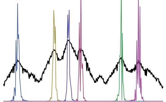
Figure 1. $f_{50}$ (black) and the plots of the absolute value of the first $6$ eigenvectors associated to the $6$ largest eigenvalues.

The value of $\alpha$ depends on the precise circumstances; larger values can lead to higher accuracy but also increase the computational cost. It is worth pointing out that it is not interesting to have $\alpha$ very large: whenever the largest eigenvalue $\lambda_{1}$ is simple and the associated eigenvector $\phi_{1}$ does not vanish, then this approach becomes less effective since

$$\lim_{\alpha\rightarrow\infty}{\frac{f_{\alpha}(k)}{\alpha}}=\bigl{\lvert}\bigl{\langle}\lambda_{1}\phi_{1},e_{k}\bigr{\rangle}\bigr{\rvert}.$$

It is not difficult to see that the convergence speed is going to depend on the spectral gap between the largest eigenvalue and the rest (in terms of absolute value of the eigenvalues)– it is commonly desirable to have a spectral gap; here, we are bound to encounter a delicate interplay between spectral gaps and the scale of localization.

2. Statament of Main result

We give one of the many possible formulation of a rigorous guarantee of the approach. Indeed, the underlying principle, as outlined in the previous section, is so simple that there are many ways of turning it into a precise statement; we give a fairly canonical one but it is by no means unique and different circumstances may call for different versions.

We start by clarifying our setup and introducing some parameters below. We first phrase everything in a way that is most natural in the setting of band matrices or matrices with rapid decay off the diagonal (which covers $-\Delta+V$ on subsets of $\mathbb{R}$, discretized by finite difference or finite volume methods) – the general case follows in a rather straightforward manner by replacing the notion of ‘interval’ by ‘subset’, we briefly discuss this below. The only restrictive assumption is the orthogonality of eigenvectors (1), which is usually given in the setting that we are interested in (localization of self-adjoint operators). (2) and (3) introduces various parameters that are always defined, however, in the non-localized regime they may result in a vacuous conclusion (see Figure 2 for an illustration).

1. The eigenvectors of $A\in\mathbb{R}^{n\times n}$ form an orthonormal basis of $\mathbb{R}^{n}$ and we order the eigenvalues via

   $$|\lambda_{1}|\geq|\lambda_{2}|\geq|\lambda_{3}|\geq\dots\geq|\lambda_{n}|.$$

2. Every one of the first $k$ eigenvectors $\phi_{i}$ has half of its $\ell^{2}-$mass supported on an interval $J_{i}\subset\left\{1,2,\dots,n\right\}$, i.e.

   $$\sum_{j\in J_{i}}{\phi_{i}(j)^{2}}\geq\frac{1}{2}$$

   and we define $\mathcal{J}$ as the longest such interval

   $$\mathcal{J}=\max_{1\leq i\leq k}{|J_{i}|}.$$

3. We assume that, for all $1\leq i\leq k$, the eigenvector $\phi_{i}$ has exponential decay away from the interval $J_{i}$, i.e. for all $1\leq i\leq k$

   $$|\left\langle\phi_{i},e_{m}\right\rangle|\leq\exp\left(-\beta\cdot\operatorname{dist}(m,J_{i})\right)$$

   for some universal constant $\beta>0$.

Figure 2. The modulus square of four eigenvectors localized in four intervals $J_{1},J_{2},J_{3},J_{4}$ bounded uniformly in length $J_{i}\leq\mathcal{J}$. The eigenvectors have exponential decay away from the intervals.

Our main result states that, depending on the size of the spectral gap and the quality of localization, there exist $\alpha,y\in\mathbb{R}$ such that the superlevel set $\left\{x:f_{\alpha}(x)\geq y\right\}$ intersects all localized intervals $J_{i}$ and $f_{\alpha}$ can only be that large in a small neighborhood of the intervals $J_{i}$. In particular, this allows for a detection of localization of the first $k$ eigenfunctions by looking at $f_{\alpha}$ alone.

Theorem.

If $\alpha\in\mathbb{N}$ is chosen such that

$$\left(\frac{\lvert\lambda_{k}\rvert}{\lvert\lambda_{k+1}\rvert}\right)^{\alpha}\geq 16\sqrt{\mathcal{J}n},$$

then there exists a critical value $y\in\mathbb{R}$ such that $f_{\alpha}$ is large on all $J_{i}$

$$\min_{1\leq i\leq k}{\max_{x\in J_{i}}{f_{\alpha}(x)}}\geq y$$

and only large in their neighborhood: if $f_{\alpha}(m)\geq y-1$, then

$$\operatorname{dist}\left(m,\bigcup_{i=1}^{k}{J_{i}}\right)\leq\frac{1}{\beta}\left(\log{\left(16\sqrt{k}\sqrt{\mathcal{J}}\right)}+\alpha\log{\left(\left|\frac{\lambda_{1}}{\lambda_{k}}\right|\right)}\right).$$

The condition on $\alpha$ depends on the spectral gap and localization properties. If the spectral gap is large, then $\alpha\sim 1$ is sufficient. If the matrix satisfies that each row has a constant number of non-zero entries (for example, if it is a local discretization of a differential operator in $d$ dimensions), this implies the computation of $f_{\alpha}$ may only require $\mathcal{O}(n)$ operations. It is clear from the proof that there are many other possible conditions under which similar result could be obtained. Natural variations include the following:

• The statement guarantees a gap of size $\geq 1$ between the values of $f_{\alpha}$ attained on the intervals and far away from their supports; in most instances a much smaller gap would suffice (especially if one identifies regions of localization via a notion of local maximum of $f_{\alpha}$, i.e., attaining a larger value than in a neighborhood of a certain size). We observe that our approach easily implies the inequalities

  $$\alpha\log{|\lambda_{1}|}-\frac{1}{2}\log{n}\leq\max_{1\leq m\leq n}{f_{\alpha}(m)}\leq\alpha\log{|\lambda_{1}|}$$

  and for any $i$

  $$\max_{m\in J_{i}}{f_{\alpha}(m)}\geq\alpha\log{|\lambda_{i}|}-\frac{1}{2}\log{n}.$$

  In combination, they suggest that the gap size $\sim 1$ could in various situations be replaced by something much smaller which would improve the error bounds.

• Orthogonality is not crucial: if the eigenvectors of $A$ form a basis and the angles between different eigenvectors are not too small, our argument easily implies similar results.

• If we know in advance that a generic localized eigenfunction is going to be roughly localized on an interval $J$ then it is clear that it suffices to compute $f_{\alpha}$ on a $\sim|\mathcal{J}|-$net which further speeds up computation time.

• $f_{\alpha}$ is defined via purely local operations and thus, by definition, its value at a certain location is stable under perturbing the matrix entries far away. On the other hand, it is entirely possible that a large perturbation will destroy the spectral structure of the matrix. With additional assumptions on the perturbation to guarantee spectral stability, it is then possible to use $f_{\alpha}$ of the unperturbed matrix to predict localization after perturbation.

We also remark that the assumptions of the theorem consists of both the existence of a gap of the spectrum and localization of the first few eigenvectors. In some situations, the localization of the eigenvectors follows from the gap assumption alone, for instance when the matrix $A$ comes from a local discretization of a differential operator, as established in [2, 13].

As $\alpha$ increases, the neighborhoods in which the result guarantees localization are growing linearly in size (though only very slowly if $|\lambda_{1}/\lambda_{k}|\sim 1$) and $f_{\alpha}(m)\geq y-1$ becomes less informative. This is not an artifact but necessary: whenever the largest eigenvalue $\lambda_{1}$ is simple and the associated eigenvector $\phi_{1}$ never vanishes, then

$$\lim_{\alpha\rightarrow\infty}{\frac{f_{\alpha}(k)}{\alpha}}=|\left\langle\lambda_{1}\phi_{1},\left(\delta_{ik}\right)_{i=1}^{n}\right\rangle|.$$

This is similar in spirit to the classical power method for computing the first eigenvector. It is noteworthy that we exploit exactly the fact that $|\lambda_{i}/\lambda_{j}|\sim 1\pm\varepsilon$ in the edge of the spectrum which makes the power method a slow method in practice. Or, put differently, our method exploits that highly localized eigenvectors associated to eigenvalues in the spectral edge correspond to metastable states for the power iteration! When $\lvert\lambda_{1}\rvert\gg\lvert\lambda_{k}\rvert$, the first eigenvector (and potentially other high lying ones) will then interfere with the performance of the procedure. In such situations, we may revise the procedure by first identifying those dominant eigenvectors and then applying the procedure while iteratively projecting onto the orthogonal complement of the subspace spanned by the dominant eigenvectors. The details are standard and left to the interested reader.

In many applications, we have the eigenvalue problem

$$Ax=\lambda x$$

with $A$ being positive definite and the dominant characteristics of the physical system being determined by the low-lying eigenvalues $\lambda$. A straightforward application of our localization technique is only going to yield the largest eigenvalues. The obvious modification is to consider the matrix

$$\mbox{Id}_{n\times n}-\frac{A}{\|A\|}\quad\mbox{instead.}$$

This operation preserves sparsity and flips the spectrum and the low-lying eigenvalues are now in the spectral edge. This is used in our numerical examples in Section 4. Alternatively, if we are given a self-adjoint, positive definite and linear map on a Hilbert space $A:H\rightarrow H$ such that $A^{-1}$ is compact, then a natural way of recovering the bottom of the spectrum is via considertion of the semigroup

$$u_{t}+Au=0.$$

An application of the spectral theorem allows us to write the semigroup as

$$e^{-tA}u=\sum_{k\geq 0}{e^{-\lambda_{k}t}\left\langle\phi_{k},u\right\rangle\phi_{k}},$$

which has slow decay for the small eigenvalues and large decay for larger eigenvalues. Note that if we Taylor expand $e^{-tA}$ and keeps only the leading order term, we get $e^{-tA}\approx\mbox{Id}-tA$, which connects with the previous trick. We refer to the Appendix A for an application.

The result, as given above, is easiest to understand in the setting of banded matrices. Banded matrices correspond naturally to localized interactions on the lattice $\mathbb{Z}$. Neighborhoods of points correspond to intervals and this is how the Theorem was phrased. At a greater level of generality, there need not be such underlying structure and we will replace intervals by general subsets $J_{i}\subset\left\{1,2,\dots,n\right\}$. The notion of distance between an element $k\in\left\{1,2,\dots,n\right\}$ and a subset $J_{i}$ is implicitly defined via assuming the inequality

$$|\left\langle\phi_{i},e_{k}\right\rangle|\leq\exp\left(-\beta\cdot\operatorname{dist}(k,J_{i})\right)$$

to hold. We emphasize that in all the interesting applications, where $A$ is the discretization of a differential operator (or somewhat localized integral operator), these notions can be made rather precise and we recover the classical notion of distance in Euclidean space.

3. Fast Randomized Algorithms

Computationally, $f_{\alpha}$ can be obtained by calculating the $\ell^{2}$-norm of the rows of the matrix $A^{\alpha}$. Thus the algorithm is particularly efficient if $A$ has structures enabling fast multiplications, such as being sparse, low rank, etc. To further accelerate the computation, we exploit the ideas from randomized numerical linear algebra (see [8] for a review) to use the following randomized version of the landscape function. For simplicity, we assume that the matrix $A$ is symmetric in this section.

Definition 2.

We define $f_{R,\alpha}:\left\{1,2,\ldots,n\right\}\rightarrow\mathbb{R}$ given by

$$f_{R,\alpha}(k)=\log\bigl{(}\lVert e_{k}^{\top}A^{\alpha}R\rVert_{\ell^{2}}\bigr{)},$$

where $\alpha\geq 0$ is a parameter, $e_{k}=(\delta_{ik})_{i=1}^{n}$ is the $k-$th standard basis vector, and $R$ is a $n\times m$ random matrix with i.i.d. $N(0,1)$ entries.

In terms of computation, if $m\ll n$, the randomized version $f_{R,\alpha}$ only requires applying the matrix $A$ on a tall skinny matrix for $\alpha$ times, and thus, the randomized version is particularly advantageous for dense $A$, as it brings down the cost from $\mathcal{O}(n^{3})$ to $\mathcal{O}(n^{2}m)$. As it turns out, the efficiency of this method is intimately coupled to very well studied concepts centered around the stability of random projection onto subspaces. To see this, we denote the columns of $R$ by $r_{1},\dots,r_{m}$ and observe that

$$\lVert e_{k}^{\top}A^{\alpha}R\rVert_{\ell^{2}}^{2}=\sum_{i=1}^{n}{\bigl{\lvert}\lambda_{i}^{\alpha}\phi_{i,k}\bigr{\rvert}^{2}\sum_{j=1}^{m}{|\left\langle\phi_{i},r_{j}\right\rangle|^{2}}},$$

while for $f_{\alpha}$, we have

$$\lVert e_{k}^{\top}A^{\alpha}\rVert^{2}=\sum_{i=1}^{n}\bigl{\lvert}\lambda_{i}^{\alpha}\phi_{i,k}\bigr{\rvert}^{2}.$$

We start by quickly discussing a very strong sufficient condition that allows to transfer results almost verbatim from our Theorem to the random case and is equivalent to classical questions in dimensionality reduction; stronger results are discussed below. We observe that certainly all the results transfer in a pointwise manner if we knew that

$$\sum_{j=1}^{m}{|\left\langle\phi_{i},r_{j}\right\rangle|^{2}}\qquad\mbox{is almost constant in the parameter}~{}i$$

for a typical realization of $m$ such random vectors. However, since the $\phi_{i}$ span the space, we are really asking that the map $h:\mathbb{S}^{n-1}\rightarrow\mathbb{R}$ given by

$$h(v)=\sum_{j=1}^{m}{|\left\langle v,r_{j}\right\rangle|^{2}}~{}\mbox{satisfies}~{}\left(1-\varepsilon\right)\frac{m}{n}\leq h(v)\leq\left(1+\varepsilon\right)\frac{m}{n}\quad\mbox{w.h.p.}$$

This is, in fact, exactly the question that underlies the study of random projections, and has been dealt with extensively (see e.g., [17]). The main conclusion is that $m\sim\log{n}$ is in many cases sufficient, however, the implicit constant may be large.

We now explain why in practice a much smaller number of random vectors suffices. The idea is rather simple and most easily explained by considering the example of one random vector in the case of a large spectral gap $\lambda_{1}\gg\lambda_{2}$. Clearly, we have

$$A^{\alpha}r=\sum_{i=1}^{n}{\lambda_{i}^{\alpha}\phi_{i}\left\langle\phi_{i},r\right\rangle}=\lambda_{1}^{\alpha}\phi_{1}\left\langle\phi_{1},r\right\rangle+\sum_{i=2}^{n}{\lambda_{i}^{\alpha}\phi_{i}\left\langle\phi_{i},r\right\rangle}.$$

The outcome now depends on the random vector $r$, however, for suitable large values of $\alpha$ it is clear that in order for the random landscape to profoundly differ from the profile of the leading eigenvector, it is required that $|\left\langle\phi_{1},r\right\rangle|$ is very small: even if it were only moderately small, it would get drastically amplified by the exponential growth and still dominate the expression. The following widely-used Lemma shows that this is not overly likely.

Lemma.

Let $v\in\mathbb{R}^{n}$ satisfy $\|v\|=1$ and let $r\in\mathbb{S}^{d-1}$ be randomly chosen w.r.t. the uniform surface measure on $\mathbb{S}^{n-1}$. Then, for $0\leq\delta\leq 1$,

$$\mathbb{P}\left(|\left\langle v,r\right\rangle|\leq\frac{\delta}{\sqrt{n}}\right)\lesssim\delta,$$

where the implicit constant depends only on the dimension.

This simple Lemma quantifies the concentration of measure phenomenon and is standard (see e.g. [9]). It explains why in the case of highly localized eigenstates it is completely sufficient to work with only one randomly chosen vector. The inner products $\left\langle\phi_{i},r\right\rangle$ are not likely to be extremely small and get amplified by an exponential growth while the strong exponential localization preserves the structure. This is easy to make precise in a variety of ways: the simplest case is a spectral gap $\lambda_{1}\gg\lambda_{2}$. The trivial estimate

$$\left\|\sum_{i=2}^{n}{\lambda_{i}^{\alpha}\phi_{i}\left\langle\phi_{i},r\right\rangle}\right\|_{\ell^{2}}\leq|\lambda_{2}|^{\alpha}\left(\sum_{i=2}^{n}{\left\langle\phi_{i},r\right\rangle^{2}}\right)^{1/2}\leq|\lambda_{2}|^{\alpha}$$

implies, together with the Lemma above,

$$\mathbb{P}\left(\left\|\lambda_{1}^{\alpha}\phi_{1}\left\langle\phi_{1},r\right\rangle\right\|_{\ell^{2}}\leq\left\|\sum_{i=2}^{n}{\lambda_{i}^{\alpha}\phi_{i}\left\langle\phi_{i},r\right\rangle}\right\|_{\ell^{2}}\right)\lesssim\sqrt{n}\left(\frac{|\lambda_{2}|}{|\lambda_{1}|}\right)^{\alpha}.$$

We emphasize that this simple argument did not even use localization of the eigenvectors; the trivial estimate is clearly quite weak if the spectrum is spread out, in that case much stronger results should hold.

Example. Let us revisit the example in Section 1.2 using the random sampling.

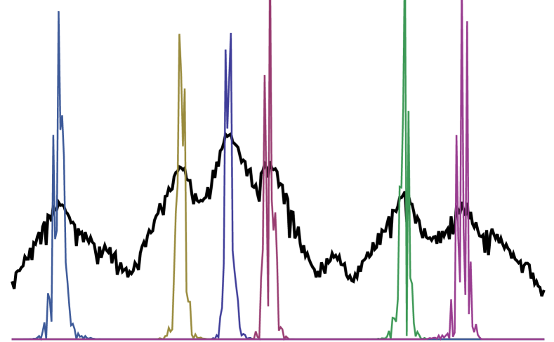
(a) $f_{50}$ without random sampling

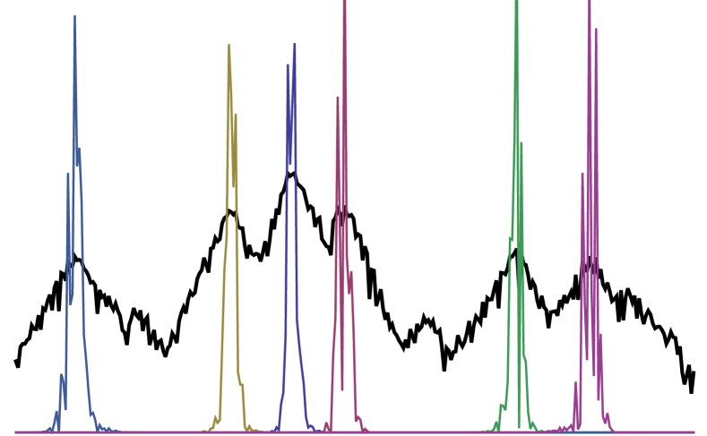
(b) $f_{R,50}$ with $1$ random vector

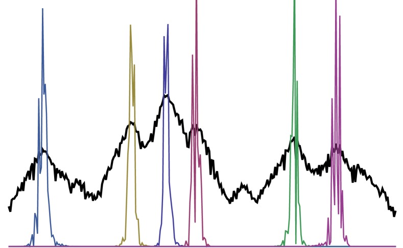
(c) $f_{R,50}$ with $3$ random vectors

(d) $f_{R,50}$ with $5$ random vectors

Figure 3. The landscape function $f_{50}$ (A), compared with its randomized sampled version with $1$ (B), $3$ (C), and $5$ (D) random vectors, are plotted in black. The absolute value of the first $6$ eigenvectors associated to the $6$ largest eigenvalues is also plotted. (A) is a replication of Figure 1.

The same random band matrix $A\in\mathbb{R}^{n\times n}$, $n=300$ for Figure 1 is used. The randomized version with number of random vectors $1$, $3$, $5$ respectively are plotted in the panels of Figure 3. We observe that the randomized landscape function even with only $1$ random vector still captures the important feature, in particular the local maxima, of the landscape function.

4. Numerical Examples

4.1. Schrödinger Operator with Potential.

The case of finding a way of numerically detecting localized eigenstates of operators of the form $-\Delta+V$ for $V\geq 0$ and Dirichlet conditions on the boundary has recently received a lot attention in the mathematics and physics literature (see e.g., [10, 11, 12, 14, 16]). We explain how our method can be applied to this case (without any restrictions on $V$). We consider the operator $-\Delta+V$ defined on $[0,1]^{2}$ with periodic boundary condition. $V$ is a smooth periodic potential generated randomly in the unit square. The pseudo-spectral discretization with mesh size $h=1/48$ is used.

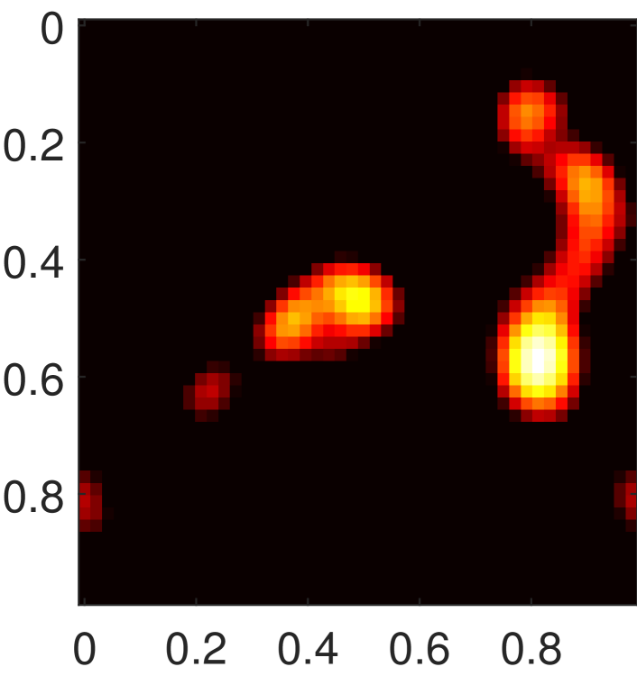
(a) $f_{R,75}$ with $10$ random vectors

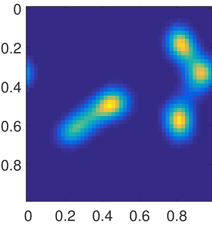
(b) Sum of modulus square: $\sum_{i=1}^{5}|\phi_{i}|^{2}$

(c) First low-lying eigenfunction $|\phi_{1}|^{2}$

(d) Second low-lying eigenfunction $|\phi_{2}|^{2}$

Figure 4. The landscape function $f_{R,75}$ (A), compared with the sum of modulus square of the low-lying $5$ eigenfunctions (B), for the operator $-\Delta+V$. The modulus square of the first two low-lying eigenfunctions are also plotted in (C) and (D) respectively.

While the resulting matrix is dense due to the Fourier differentiation of the pseudo-spectral method, the method proposed still applies. In Figure 4, we show the landscape function using $\alpha=75$ and $10$ random vectors on the left panel and the sum of the square modulus of the low-lying $5$ eigenvectors on the right panel. Good agreement is observed. For visualization, we only plotted the part of landscape function exceeding its maximum value minus $1$.

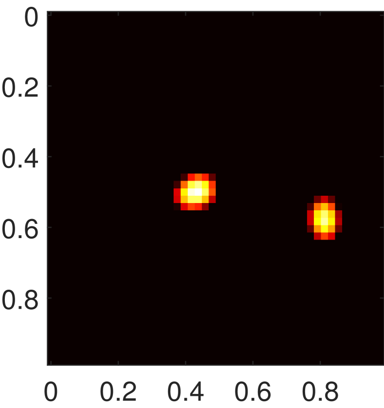
(a) $f_{R,75}$ with $10$ random vectors

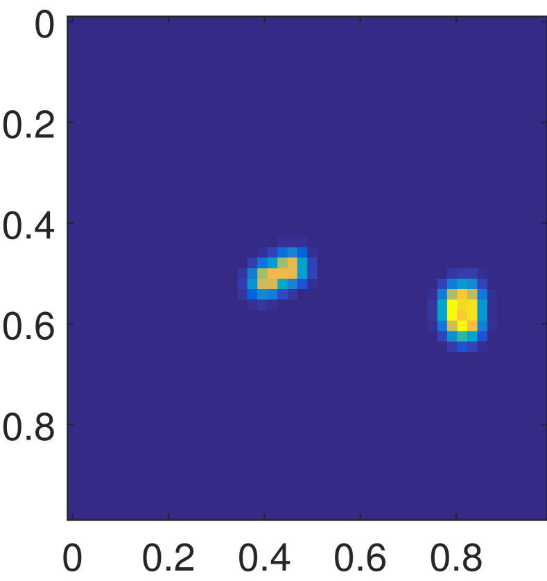
(b) Sum of modulus square: $\sum_{i=1}^{5}|\phi_{i}|^{2}$

(c) First low-lying eigenfunction $|\phi_{1}|^{2}$

(d) Second low-lying eigenfunction $|\phi_{2}|^{2}$

Figure 5. The landscape function $f_{R,75}$ (A), compared with the sum of modulus square of the low-lying $5$ eigenfunctions (B), for the operator $(-\Delta)^{3/4}+V$. The same potential as in the example of Figure 4 is used. The modulus square of the first two low-lying eigenfunctions are also plotted in (C) and (D) respectively.

4.2. Fractional Laplacian

The method extends without much difficulty to the fractional Laplacian $(-\Delta)^{s}+V$. We still consider the computational domain $[0,1]^{2}$ with periodic boundary condition and $V$ a smooth randomly generated potential. Thanks to the periodic boundary condition, the fractional Laplacian $(-\Delta)^{s}$ can be defined through spectral decomposition. Pseudo-spectral discretization is again used. Note that the fractional Laplacian is non-local, regardless of the discretization. In Figure 5, we show the result for $(-\Delta)^{3/4}+V$ where the same potential as in the example of Figure 4 is used. We again observe excellent agreement between the landscape function and the localization of the eigenfunctions.

5. Proofs

Proof of the Theorem.

We first show that $f_{\alpha}$ exceeds a certain value on all the intervals $J_{i}$ ($1\leq i\leq k$). We start by showing there is a $k\in J_{i}$ with

$$\left|\left\langle\phi_{i},e_{k}\right\rangle\right|\geq\frac{1}{2}\frac{1}{\sqrt{\mathcal{J}}}.$$

If this were false, then

$$\frac{1}{4}\leq\sum_{k\in J_{i}}{\left|\left\langle\phi_{i},e_{k}\right\rangle\right|^{2}}<\sum_{k\in J_{i}}{\frac{1}{4J}}=\frac{|J_{i}|}{4\mathcal{J}}\leq\frac{1}{4},$$

which is a contradiction. Here the first inequality comes from the assumption that $J_{i}$ contains half $\ell^{2}$-mass of $\phi_{i}$. A simple application of the spectral theorem implies that

$$\|A^{\alpha}e_{k}\|_{\ell^{2}}\geq\frac{1}{2\sqrt{\mathcal{J}}}|\lambda_{i}|^{\alpha}\geq\frac{1}{2\sqrt{\mathcal{J}}}|\lambda_{k}|^{\alpha}.$$

It remains to show that this value cannot be attained unless one is close to one of the localized eigenvectors. If $m\in\left\{1,2,\dots,n\right\}$ has at least distance $d>0$ from $\bigcup_{i=1}^{k}{J_{i}},$ then

$$\|A^{\alpha}e_{m}\|^{2}_{\ell^{2}} =\sum_{l=1}^{n}{\left|\left\langle e_{m},\phi_{l}\right\rangle\right|^{2}|\lambda_{l}|^{2\alpha}}\leq e^{-2\beta d}k|\lambda_{1}|^{2\alpha}+n|\lambda_{k+1}|^{2\alpha}$$

and thus

$$\|A^{\alpha}e_{m}\|_{\ell^{2}}\leq e^{-\beta d}\sqrt{k}|\lambda_{1}|^{\alpha}+\sqrt{n}|\lambda_{k+1}|^{\alpha}.$$

We want to relate this to the inequality

$$e^{-\beta d}\sqrt{k}|\lambda_{1}|^{\alpha}+\sqrt{n}\left(|\lambda_{k+1}|\right)^{\alpha}\leq\frac{1}{4}\left(\frac{1}{2\sqrt{\mathcal{J}}}|\lambda_{k}|^{\alpha}\right),$$

which will provide an upper bound on $d$ (meaning that if the distance is to the sets is larger than this bound, then we obtain the desired consequence). If, as we assume,

$$\left(\frac{\lvert\lambda_{k}\rvert}{\lvert\lambda_{k+1}\rvert}\right)^{\alpha}\geq 16\sqrt{\mathcal{J}n}\qquad\mbox{then}\qquad\sqrt{n}\left(|\lambda_{k+1}|\right)^{\alpha}\leq\frac{1}{8}\left(\frac{1}{2\sqrt{\mathcal{J}}}|\lambda_{k}|^{\alpha}\right).$$

The inequality

$$e^{-\beta d}\sqrt{k}|\lambda_{1}|^{\alpha}\leq\frac{1}{8}\left(\frac{1}{2\sqrt{\mathcal{J}}}|\lambda_{k}|^{\alpha}\right)$$

is equivalent to

$$d\leq\frac{1}{\beta}\left(\log{\left(16\sqrt{k}\sqrt{\mathcal{J}}\right)}+\alpha\log{\left(\left|\frac{\lambda_{1}}{\lambda_{k}}\right|\right)}\right)$$

which is the desired statement. ∎

Appendix A Localized Wannier Bases

In this appendix, we connect the landscape functions to localized Wannier bases. Localized Wannier bases [18] are maximally localized bases of low-lying eigenfunctions. Give an operator over $\Omega$ with mutually orthogonal low-lying eigenfunctions $\phi_{1},\dots,\phi_{n}\in L^{2}(\Omega)$, it is often helpful to work with a basis of $\mbox{span}\left\{\phi_{1},\dots,\phi_{n}\right\}$ where each basis element is as localized as possible (for example to obtain sparser matrices). A classical approach, see e.g., the review article [15], is to simply project the Dirac measure $\delta_{x}$ onto the finite-dimensional subspace $\mbox{span}\left\{\phi_{1},\dots,\phi_{n}\right\}$ to obtain the best possible representation of this localized point in the basis. We illustrate this with a simple example: let us consider $\left\{e^{-inx},e^{-i(n-1)x},\dots,1,\dots,e^{inx}\right\}$ on the torus $\mathbb{T}$. The projection of $\delta_{y}$ onto the span is given by

$$\pi_{n}\delta_{y}=\sum_{k}{\left\langle\delta_{y},\phi_{k}\right\rangle\phi_{k}}=\sum_{k=-n}^{n}{e^{iky}e^{-ikx}}=\sum_{k=-n}^{n}{e^{ik(x+y)}}=\frac{\sin{\left(\left(n+\frac{1}{2}\right)(x-y)\right)}}{\sin{(x-y)/2}},$$

which is merely the classical Dirichlet kernel. The function is indeed highly localized around $y$, roughly constant for $|x-y|\lesssim n^{-1}$ and then exhibits some oscillatory behavior around 0 further away from $y$. Motivated by our main idea, a slightly different idea suggests itself: instead of merely projecting, it makes sense to run the dynamical system with $\delta_{y}$ as initial datum on the subspace on which we project. More precisely, this yields a projection that depends on $t$

$$\pi_{n,t}\delta y:=\sum_{k}{e^{-\lambda_{k}t}\left\langle\delta_{y},\phi_{k}\right\rangle\phi_{k}}.$$

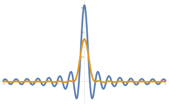
Figure 6. The projection on $\mathbb{T}$ for $n=15$ and the parametrized projection with $t=0.01$. We observe a tradeoff between localization and decay.

Basic intuition tells us that, depending on the speed of propagation within the dynamical system, at least for small values of $t$ the projection will still look pretty much like the direct propagation. Our main observation is that for sufficiently small values of $t$, the projection $\pi_{n,t}$ will be pretty much as localized as $\pi_{n}$ but will have much better decay properties. We illustrate this again on the torus $\mathbb{T}$, where

$$pi_{n,t}\delta y:=\sum_{k}{e^{-\lambda_{k}t}\left\langle\delta_{y},\phi_{k}\right\rangle\phi_{k}}=\sum_{k}{e^{-k^{2}t}e^{-iky}e^{ikx}}.$$

We observe that the infinite limit is given by the Jacobi $\theta-$function

$$\theta_{t}(x-y)=\sum_{k=\infty}^{\infty}{e^{-k^{2}t}e^{ik(x-y)}}.$$

The Jacobi $\theta-$function has exponential decay in the region $|x-y|\gtrsim t^{1/2}$ and, what is especially useful, the exponential decay in the coefficients implies that a cutoff at frequency $n$ is only going to introduce a small error. In particular, in this setting, the threshold-value for $t$ (where localization properties are not significantly worse) is $t\lesssim n^{-2}$. This example generalizes immediately to higher-dimensions, where the situation is more or less identical: the direct projection $\pi_{n}$ creates oscillations with slow decay throughout the entire space, the diffused $\pi_{n,t}$ leads to a more localized representation. Returning to our original problem for matrices $A\in\mathbb{R}^{n\times n}$, the relationship to $f_{\alpha}$ is easily explained: in the case of localized eigenvectors, we see that if $\phi$ is the eigenvector associated to the largest eigenvalue on coordinate $k\in\left\{1,2,\dots,n\right\}$, then $A^{\alpha}\left(\delta_{ik}\right)_{i=1}^{n}$ is a very good local approximation of $\phi$. The proof of this simple statement proceeds along the very same lines as the proof of our main theorem.

References

- [1] P. W. Anderson, Absence of Diffusion in Certain Random Lattices, Phys. Rev. 109 (1958), 1492–1505.
- [2] M. Benzi, P. Boito, and N. Razouk, Decay properties of spectral projectors with applications to electronic structure, SIAM Rev. 55 (2013), 3–64.
- [3] A. Bovier, M. Eckhoff, V. Gayrard and M. Klein, Metastability and low lying spectra in reversible Markov chains. Comm. Math. Phys. 228 (2002), no. 2, 219–255.
- [4] A. Bovier, M. Eckhoff, V. Gayrard, and M. Klein, Metastability in reversible diffusion processes. I. Sharp asymptotics for capacities and exit times. J. Eur. Math. Soc. 6 (2004), no. 4, 399–424.
- [5] A. Bovier, V. Gayrard and M. Klein, Metastability in reversible diffusion processes. II. Precise asymptotics for small eigenvalues. J. Eur. Math. Soc. 7 (2005), no. 1, 69–99.
- [6] X. Cheng, M. Rachh and S. Steinerberger, On the Diffusion Geometry of Graph Laplacians and Applications, preprint, arXiv:1611.03033.
- [7] Weinan E, Tiejun Li, and Jianfeng Lu, Localized bases of eigensubspaces and operator compression, Proc. Natl. Acad. Sci. USA, 107 (2010), 1273–1278.
- [8] N. Halko, P. G. Martinsson, and J. A. Tropp, Finding Structure with Randomness: Probabilistic Algorithms for Constructing Approximate Matrix Decompositions, SIAM Rev. (2011), 53(2), 217–288.
- [9] C. Kenney and A. Laub, Small-sample statistical condition estimates for general matrix functions. SIAM J. Sci. Comput. 15 (1994), no. 1, 36–61.
- [10] G. Lefebvre, A. Gondel, M. Dubois, M. Atlan, F. Feppon, A. Labbe, C. Gillot, A. Garelli, M. Ernoult, S. Mayboroda, M. Filoche, P. Sebbah, One single static measurement predicts wave localization in complex structures, Phys. Rev. Lett. 117 (2016), 074301.
- [11] M. Filoche and S. Mayboroda, Universal mechanism for Anderson and weak localization. Proc. Natl. Acad. Sci. USA 109 (2012), no. 37, 14761-14766.
- [12] M. Filoche and S. Mayboroda, The landscape of Anderson localization in a disordered medium, Contemporary Mathematics, 601 (2013), 113–121.
- [13] L. Lin and J. Lu, Decay estimates of discretized Green’s functions for Schrödinger type operators, Sci. China Math. 59 (2016) 1561–1578.
- [14] M. Lyra, S. Mayboroda and M. Filoche, Dual hidden landscapes in Anderson localization on discrete lattices, Euro. Phys. Lett. 109 (2015), 4700.
- [15] N. Marzari, A. A. Mostofi, J. R. Yates, I. Souza, D. Vanderbilt, Maximally localized Wannier functions: Theory and applications, Rev. Mod. Phys. 84 (2012), 1419–1475.
- [16] S. Steinerberger, Localization of Quantum States and Landscape Functions, Proc. Amer. Math. Soc, accepted.
- [17] S. Vempala, The random projection method. With a foreword by Christos H. Papadimitriou. DIMACS Series in Discrete Mathematics and Theoretical Computer Science, 65. American Mathematical Society, Providence, RI, 2004.
- [18] G. Wannier, The Structure of Electronic Excitation Levels in Insulating Crystals, Phys. Rev. 52 (1937), 191.
- [19] H. Zou, T. Hastie, R. Tibshirani, Sparse principal component analysis, J. Comput. Graph. Stat. 15 (2006), 262–286.