Abstract

A standard approach to reduce the complexity of very large networks is to group together sets of nodes into clusters according to some criterion which reflects certain structural properties of the network. Beyond the well-known modularity measures defining communities, there are criteria based on the existence of similar or identical connection patterns of a node or sets of nodes to the remainder of the network; this approach supports so-called positional analyses and the definition of certain structures in social, commercial and economic networks. A key notion in this context is that of structurally equivalent or twin nodes, displaying exactly the same connection pattern to the remainder of the network.

The first goal of this paper is to extend this idea to subgraphs of arbitrary order of a given network, by means of the notions of T-twin and F-twin subgraphs. This research, which leads to graph-theoretic results of independent interest, is motivated by the need to provide a systematic approach to the analysis of core-semiperiphery-periphery (CSP) structures, a notion which is widely used in network theory but that somehow lacks a formal treatment in the literature. The goal is to provide an analytical framework accommodating and extending the idea that the unique (ideal) core-periphery (CP) structure is a 2-partitioned $K_{2}$, a fact which is here understood to rely on the true-twin and false-twin notions for vertices already known in network theory. We provide a formal definition of such CSP structures in terms of core eccentricities and periphery degrees, with semiperiphery vertices acting as intermediaries between both. The T-twin and F-twin notions then make it possible to reduce the large number of resulting structures by identifying isomorphic substructures which share the connection pattern to the remainder of the graph, paving the way for the decomposition and enumeration of CSP structures. We compute explicitly the resulting CSP structures up to order six.

We illustrate the scope of our results by analyzing a subnetwork of the well-known network of metal manufactures trade arising from 1994 world trade statistics. As this example suggests, our approach can be naturally applied in complex network theory and seem to have many potential extensions, since the analytical properties of twin subgraphs and the structure of CSP and other partitioned graphs admit further study.

Keywords: graph, network, twin, structural equivalence, core-periphery, core-semiperiphery-periphery.   AMS Subject Classification: 05C50, 05C82, 90B10, 91D30, 94C15.

1 Introduction

The notion of a core-periphery (CP) structure can be traced back at least to some research on economic and commercial networks developed in the late 1970s and early 1980s [14, 32, 36], largely emanating from the influential work of Wallerstein on world systems analysis [37]. These ideas were revisited and addressed in a more formal framework by Borgatti and Everett in [8]. For these authors, the two key ideas in the definition of a core-periphery structure in a network context are those of a dense, cohesive core of heavily interconnected nodes and a sparse periphery of nodes, essentially lacking any connections among them; by contrast, the connection pattern between the core and the periphery admits several definitions and, actually, the core-periphery connection densities differ from some models to others. In idealized models, core nodes are fully connected among them, periphery nodes are isolated (within the periphery subnetwork), whereas the core and the periphery may either be fully connected or totally disconnected. Since then, a great deal of research has been directed to the detection of such core-periphery structures in real networks, measuring how well they approximate the ideal ones, and to the development of analytical and computational tools to classify nodes in such networks (cf. [9, 17, 18, 26, 27, 34, 38] and references therein). Other approaches to the definition of a core-periphery structure can be found in [13, 16, 22].

Even though the idea of a core-semiperiphery-periphery (CSP) structure can be also found in the aforementioned sociological works (cf. [36, 37]), and despite the fact that this concept has been widely used since then (see e.g. [18, 19, 30, 34]), the network literature seems to lack a formal definition and a systematic classification of these CSP structures. In the aforementioned paper by Borgatti and Everett [8], these authors indicate that there are many reasonable options to define a CSP structure and, further, discrete partitions with more than three classes. The difficulty does not seem to rely on providing a formal definition but on classifying the resulting “reasonable options”, quoting these authors; more precisely, there is a need for a notion of similar or equivalent subgraphs making it possible to somehow reduce the number of different CSP structures. When dealing with core-periphery structures, there is a well-known subgraph similarity notion which makes this reduction feasible, namely, that of structural equivalence defining so-called twin nodes (broadly, two vertices are twins if they have the same neighbors; a distinction is made between true twins and false twins depending on whether both vertices are adjacent or not; details are given in Section 2). Essentially, under structural equivalence, $K_{2}$ will be the unique core-periphery structure: details are provided later, but the reader can think for the moment e.g. in the star $S_{n}$ as a network with a unique core (the central node) to whom $n-1$ peripheric nodes are attached; all $n-1$ leaves have the same set of neighbors -namely, the central node- and are therefore structurally equivalent (more precisely, they will be false twins); then, after identifying all leaves in light of this twin notion for vertices, the quotient graph amounts to $K_{2}$.

But in the network literature there is no equivalence notion for “similar” higher order subgraphs, which would pave the way to a systematic reduction of (eventually defined) CSP structures. As explained in detail in Section 2 (see, specifically, subsection 2.3), the goal of this paper is to fill this gap by introducing a mathematical framework allowing for a systematic classification of CSP networks and other partitioned structures. The key idea is to introduce the concept of twin subgraphs, a notion which extends to arbitrary order that of twin (structurally equivalent) vertices. This mathematical framework will be developed in Sections 3 and 4, which address graph-theoretic problems of independent interest (that is, problems which go beyond the eventual application of these notions to the classification of CSP structures). These sections introduce and elaborate on the idea of F-twin and T-twin subgraphs, which in a sense are dual to each other and generalize several known properties of false twin and true twin vertices; e.g. distinct connected components of F-twin pairs will be proved to be disjoint and non-adjacent, whereas disjoint T-twin pairs will be fully connected to each other. With this background, the classification of CSP networks will then be tackled in Section 5. In Section 6 we present the lines along which these structures can be identified in real cases by analyzing a subnetwork of the network of manufactures of metal arising from 1994 world trade statistics. These data are available and analyzed in [19], in the spirit of the the aforementioned seminal work [37], and nowadays define a widely used benchmark for the positional analyses of networks. Finally, Section 7 compiles some lines for future research.

2 Background on graphs, twins, and core-periphery networks

2.1 Graph-theoretic notions

We refer the reader to [5, 6, 20, 23] for excellent introductions to graph theory. Throughout the paper we will work with undirected graphs ${\cal G}=(V,E)$ without parallel edges or self-loops, so that edges can be thought of as pairs of distinct vertices (also termed nodes). Given a graph ${\cal G}$, its vertex and edge sets will be written as $V({\cal G})$ and $E({\cal G})$, respectively, or simply as $V$ and $E$ if there is no possible ambiguity. We will only work with finite graphs, that is, the order (number of vertices) will be finite in all cases. With notational abuse, we will often write $v\in{\cal G}$ to mean $v\in V({\cal G})$ and $V_{0}\subseteq{\cal G}$ for $V_{0}\subseteq V({\cal G})$. Analogously, we will say that two graphs are disjoint when their vertex sets are disjoint (note that the latter implies that the edge sets are disjoint as well).

A path of length $k\geq 0$ is a graph with $k+1$ distinct vertices $v_{0},$ $v_{1},\ldots,v_{k}$ and edges $e_{1},\ldots,e_{k}$ with $e_{i}$ joining $v_{i-1}$ and $v_{i}$. Since we are not allowing parallel edges, a path is uniquely defined by its vertex set. We say that $v_{0}$ and $v_{k}$ are linked by such a path. When $k\geq 1$, sometimes the vertex set will be implicitly assumed to inherit the order defined by the indices and we will then speak of a path from $v_{0}$ to $v_{k}$. The distance, $d$, between a pair of distinct vertices in the same connected component of a given graph is the length of a shortest path linking them. The eccentricity of a vertex in a connected graph is the maximum distance to other vertices. The distance between two disjoint subgraphs $H_{1}$ and $H_{2}$ lying in the same connected component of a given graph is defined as ${\rm min}\{d(u,v),\ u\in H_{1}$, $v\in H_{2}\}$. We say that two disjoint subgraphs $H_{1}$ and $H_{2}$ are not adjacent if there is no adjacent pair $(u,v)$ with $u\in H_{1}$, $v\in H_{2}$; if both subgraphs lie in the same connected component of ${\cal G}$, this is equivalent to saying that $d(H_{1},H_{2})\geq 2$.

We will denote by ${\cal N}(u)$ the set of neighbors of a given vertex $u$ (namely, the set of vertices adjacent to $u$), and write ${\cal N}[u]={\cal N}(u)\cup\{u\}$. The degree of a vertex $u$ is the number of elements in ${\cal N}(u)$. We will call a vertex of degree one a leaf (note that this term is often reserved to cases in which the whole graph is acyclic, that is, a disjoint union of trees), and will say that it is attached to its unique adjacent vertex.

The null graph defined by $V=\emptyset$ will be denoted by $K_{0}$; $K_{n}$ with $n\geq 1$ stands for the complete graph on $n$ vertices. The complement of a graph ${\cal G}=(V,E)$ of order $n$ (namely, $(V,E(K_{n})-E)$) will be written as $\overline{\cal G}$, and $E_{n}$ will stand for the empty graph $\overline{K_{n}}$ on $n\geq 1$ vertices. Cycles, paths and stars on $n$ vertices will be written as $C_{n}$, $P_{n}$ and $S_{n}$, respectively, with $n\geq 3$ for cycles. As usual, the union and intersection of ${\cal G}_{i}=(V_{i},E_{i})$ ($i=1,$ $2$) are the graphs $(V_{1}\cup V_{2},E_{1}\cup E_{2})$ and $(V_{1}\cap V_{2},E_{1}\cap E_{2})$, respectively. The join ${\cal G}_{1}+{\cal G}_{2}$ of two graphs with disjoint vertex sets $V({\cal G}_{1})$, $V({\cal G}_{2})$ is the graph obtained after enlarging ${\cal G}_{1}\cup{\cal G}_{2}$ with all possible edges joining the vertices of ${\cal G}_{1}$ to those of ${\cal G}_{2}$ (sometimes we express the latter by saying that ${\cal G}_{1}$ and ${\cal G}_{2}$ are fully connected to one another).

A partitioned graph is simply a graph whose vertex set is split into (pairwise disjoint) classes. A $k$-partitioned graph is a partitioned graph with $k$ non-empty partition classes. Obviously, a partitioned graph defines an equivalence relation in the set of vertices. The quotient graph (often called a supergraph) of a partitioned graph is defined as a graph whose vertex set is the quotient set (that is, vertices in the quotient graph correspond to the partition classes in the original graph), two distinct vertices in the quotient being adjacent if and only if the original graph has at least one edge which joins vertices belonging to the corresponding pair of classes.

An isomorphism of two graphs ${\cal G}_{1}$ and ${\cal G}_{2}$ is a bijection $\varphi:V_{1}\to V_{2}$ (with $V_{i}=V({\cal G}_{i})$) which preserves adjacencies, that is, such that any given pair of vertices $u$, $v$ in ${\cal G}_{1}$ are adjacent if and only if $\varphi(u)$ and $\varphi(v)$ are adjacent in ${\cal G}_{2}$. An isomorphism of partitioned graphs is a graph isomorphism which keeps the classes invariant.

2.2 Twins

Different analytical and computational issues arise in connection to the existence and the distribution of isomorphic copies of certain subgraphs of a given graph: see e.g. [2, 15, 21, 23, 31] and references therein. From a different perspective, some attention has been focused on vertices which share the same connection pattern within a graph. Such vertices receive (at least) two different names in the literature, namely, twins and structurally equivalent vertices, as detailed in the sequel. Two (distinct) vertices $u$ and $v$ are false twins (resp. true twins) if ${\cal N}(u)={\cal N}(v)$ (resp. ${\cal N}[u]={\cal N}[v]$) [4, 11, 25, 29]. The exclusion of self-loops yields $u\notin{\cal N}(u)$ and this implies that false twins are not adjacent. In the dual case, true twins are necessarily adjacent to each other: for these reasons, true and false twins are also called adjacent and non-adjacent twins (see e.g. [4, 24, 29]). True twins correspond to 1-twins in the terminology of [12, 28]. By contrast, in the social network analysis literature twin vertices $u$ and $v$ are said to be (weakly) structurally equivalent: this means that the transposition $t_{u,v}$ of $u$ and $v$ yields an automorphism of the graph (cf. [7, 10]), a condition which is easily seen equivalent to $u$ and $v$ being (false or true) twins in the sense indicated above.

The F-twin and T-twin notions that will be introduced in Sections 3 and 4 for arbitrary subgraphs somehow combine the two ideas at the beginning of the paragraph above. Twin subgraphs will be isomorphic copies of each other and, additionally, they will share the connection pattern to the remainder of the graph; in other words, our approach will define a structural equivalence notion for (isomorphic) subgraphs which extends the one already defined for single vertices. Consistently, twin subgraphs will retain, mutatis mutandis, certain properties already known for twin vertices, such as the aforementioned adjacency properties (which will hold for disjoint twin subgraphs; cf. Corollaries 2 and 6), the duality between F-twins and T-twins in the sense that a pair of twins of one type defines a pair of the other on the complement graph (Theorem 2), or the fact that twins will have the same distance multisets to the vertex set of the graph (cf. Proposition 4). In particular, twin subgraphs will define homometric sets (Corollary 3; cf. [1, 3, 35]). Both notions will induce a classification in the family of isomorphic copies of each induced subgraph, extending the way in which false and true twin concepts classify the vertices of a graph. These, together with other related results, will be extensively discussed in Sections 3 and 4.

2.3 Core-periphery networks

Consider one of the “idealized” core-periphery (CP) networks mentioned in Section 1, namely, the one defined by a 2-partitioned graph with the following two classes of vertices:

• core vertices, which are fully connected to each other and also to the vertices in the second class (defined below);

• periphery vertices, totally disconnected from each other (and fully connected to the core, in light of the first requirement above).

As indicated in the Introduction, other core-periphery connection patterns are possible, although the one above is often used as a starting point in different analytical and computational approaches to this topic (see e.g. [8, 19]). These core-periphery networks are simply 2-partitioned graphs of the form $K_{p}+E_{r}$ (find notations in subsection 2.1; when using a 2-partitioned structure in $K_{p}+E_{r}$, we assume throughout the document and without further mention that the two partition classes are the vertex sets of $K_{p}$ and $E_{r}$). Cases with a unique core vertex amount to the star $S_{n}=K_{1,n-1}=K_{1}+E_{n-1}$. In the simplest setting ($n=2$) we get a 2-partitioned $S_{2}=K_{2}=K_{1}+K_{1}$, with a single core and a single periphery vertex; note that $E_{1}=K_{1}$, and we prefer to use the latter notation for the singleton graph.

Aiming at later developments let us note that, in a certain sense, $K_{2}$ is substantially different from all other joins $K_{p}+E_{r}$. Actually, we may think of $K_{2}=K_{1}+K_{1}$ as the quotient graph of any other join of the form $K_{p}+E_{r}$. But, in order to extend these ideas to support the definition and classification of more complex structures, we emphasize that the reduction above comprises more than a quotient reduction. Indeed, all core vertices (namely, those of $K_{p}$) are true twins as defined in subsection 2.2 above and, analogously, all periphery vertices (the ones in $E_{r}$) are false twins. In this context, $K_{2}$ arises not only as the reduction of other joins, but also as the unique twin-free network meeting the requirements (i) and (ii) above. From this point of view we may think of $K_{2}$ as the unique core-periphery structure (we use the latter term to make a distinction with the CP networks $K_{p}+E_{r}$ above, which are allowed to display twin vertices). To avoid any misunderstanding, let us clarify that $K_{2}$ is twin-free only as a 2-partitioned graph, that is, we cannot consider both vertices as (true) twins because they belong to different partition classes; cf. the beginning of Section 5.

However, when scaling these ideas to define formally core-semiperiphery-periphery (CSP) structures, and eventually other structures with more partition classes, one finds the problem that there is no appropriate analog of the twin notions mentioned above for subgraphs with more than one vertex. Since the intuitive idea behind the concept of a core is that of a set of heavily connected vertices, the true-twin notion for single vertices may well apply to reduce the number of admissible core subgraphs in these higher order structures; by contrast, in the literature one finds no way to reduce conveniently the semiperiphery-periphery subgraph.

To put it in the simplest possible setting, compare the CP network $K_{1}+E_{2}$ (Fig. 1(a)), which amounts to a 2-partitioned path $P_{3}$ with one class (the core, painted black in the figure) defined by the central node, with a 3-partitioned path $P_{5}$ in which the three classes are defined by the central vertex (core), the two vertices with eccentricity three (semiperiphery vertices, grey) and the two leaves (periphery vertices, white) (Fig. 1(b)). We may think of the latter as a (sometimes called) spider graph with a central vertex (the core) and two legs, each one a $P_{2}=K_{2}$ attached to the core by a single articulation (the semiperiphery vertices).

                                                             

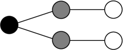
Figure 1:   (a) CP network $K_{1}+E_{2}$                       (b) A spider                               

As indicated above, in the CP case ($K_{1}+E_{2}$) the false twin notion makes it possible to identify the two peripheries into a single one, reducing the network to a 2-partitioned $K_{2}=P_{2}$ (cf. Fig. 2(a)). But, how can we reduce the CSP case (the spider) to a single $P_{3}$, which captures the essential connection pattern? (Fig. 2(b)). Note that both legs in Fig. 1(b) have exactly the same structure and, accordingly, we should find a systematic way to perform such reduction. Note also that neither the semiperiphery vertices nor the periphery ones in Fig. 1(b) are false twins, so that an eventual recourse to the notion of twin vertices would fail for our present purpose.

                                                             

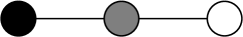
Figure 2:   (a) CP structure                            (b) CSP structure                         

Obviously, it would be easy to identify equal-length legs in spider graphs; however, more complex structures are possible: think e.g. of cases with more cores and/or with other connection patterns within the semiperiphery (actually, different CSP structures will arise in Sections 5 and 6; see Figs. 3-8). Additionally, the goal should be the development of a broader mathematical framework allowing for an identification of (say) structurally equivalent, higher order subgraphs in greater generality. The idea is to formalize the notion of isomorphic subgraphs or arbitrary order displaying, in a sense to be made precise, the same connection patterns to the remainder of the graph, generalizing the false-twin and true-twin concepts for single vertices. The F-twin notion for arbitrary subgraphs, together with the dual concept of T-twin subgraphs, are aimed at filling this gap. After introducing and discussing these ideas in Sections 3 and 4, we will be back to CSP structures in Sections 5 and 6.

3 F-twin subgraphs

3.1 Definition and elementary properties

Definition 1.

Let $H_{1}$ and $H_{2}$ be two induced subgraphs of a graph ${\cal G}$. Denote by $V_{i}$ the vertex set of $H_{i}$. $H_{1}$ and $H_{2}$ are called F-twins if they are isomorphic via a map $\varphi:V_{1}\to V_{2}$ for which the identities

$${\cal N}(u)-V_{1}={\cal N}(\varphi(u))-V_{2}$$ (1)

hold for all $u\in V_{1}.$

We may also say that the set of vertices $V_{1}$ and $V_{2}$ are F-twins, since the definition above requires $H_{1}$ and $H_{2}$ to be the subgraphs induced by $V_{1}$ and $V_{2}$ and there is no possible ambiguity. The reason for the requirement that F-twins are induced subgraphs should become apparent in light of a simple example, defined by the graph ${\cal G}=P_{3}\cup K_{3}$. Let $H_{1}$ be the $P_{3}$-component of ${\cal G}$ and $H_{2}$ any one of the three subgraphs of $K_{3}$ isomorphic to $P_{3}$. Should F-twins not be required to be induced subgraphs, $H_{1}$ and $H_{2}$ would be F-twins, because the identities (1) hold trivially since both sides are empty for all vertices. However there exists an extra edge in $K_{3}$ which make the endvertices of $H_{2}$ adjacent in ${\cal G}$ without the endvertices of $H_{1}$ being so. Since the idea of the F-twin notion is to capture identical adjacency patterns, we rule out this type of situations by requiring $H_{1}$ and $H_{2}$ to be induced subgraphs.

Note that any induced subgraph is trivially an F-twin of itself; we will say that a given induced subgraph is a proper F-twin if it has at least an F-twin different from itself (and both of them will also be said to be proper F-twins of each other). A trivial F-twin is an induced subgraph that has no F-twin but itself.

In particular, the notion above for two single distinct vertices $u$, $v$ amounts to requiring that they are false twins in the sense that ${\cal N}(u)={\cal N}(v)$, as defined in subsection 2.2. Just note that $u\not\in{\cal N}(u)$ and $v\not\in{\cal N}(v)$, so that (1) holds in this case if and only if ${\cal N}(u)={\cal N}(v)$.

Proposition 1.

Two induced subgraphs $H_{1}$ and $H_{2}$ are F-twins if and only if their connected components can be matched as pairs of F-twins.

Proof. Assume first that $H_{1}$ and $H_{2}$ are F-twins, and let $\varphi$ denote the isomorphism arising in Definition 1. Then $\varphi$ induces $k$ isomorphisms $\varphi_{1},\ \ldots,\varphi_{k}$ between the connected components of $H_{1}$ and $H_{2}$; denote these connected components by $H_{i,j}$, with $i\in\{1,2\},\ j\in\{1,\ldots,k\}$, and let accordingly $V_{i,j}$ be the vertex set of $H_{i,j}$, so that $\varphi_{j}:V_{1,j}\to V_{2,j}$. Then obviously

$$V_{i}=\bigcup_{j=1}^{k}V_{i,j}$$

and, provided that a vertex $u$ (resp. $\varphi(u)$) belongs to $V_{1,j}$ (resp. to $V_{2,j}$), it is also clear that ${\cal N}(u)\cap V_{1}\subseteq V_{1,j}$, which implies ${\cal N}(u)\cap V_{1,k}=\emptyset$ if $k\neq j$ (resp. ${\cal N}(\varphi(u))\cap V_{2}\subseteq V_{2,j}$ and then ${\cal N}(\varphi(u))\cap V_{2,k}=\emptyset$ if $k\neq j$). This yields

$${\cal N}(u)-V_{1,j}={\cal N}(u)-V_{1}={\cal N}(\varphi(u))-V_{2}={\cal N}(\varphi_{j}(u))-V_{2,j}$$ (2)

so that $H_{1,j}$ and $H_{2,j}$ are indeed F-twins.

The converse result proceeds in exactly the same manner and details are left to the reader.

$\Box$

The result above is non-trivial only when $H_{1}$ and $H_{2}$ are not connected. In this setting, even if $H_{1}$ and $H_{2}$ are proper F-twins some of their components might be trivial F-twins.

Proposition 2.

If $H_{1}$ and $H_{2}$ are proper F-twins, the intersection $V_{1}\cap V_{2}$, if non-empty, induces a set of connected components of both $H_{1}$ and $H_{2}$.

Proof. Assume that $w\in V_{1}\cap V_{2}$, and let $K_{1}$ and $K_{2}$ be the connected components of $H_{1}$ and $H_{2}$ which accommodate $w$. Assume that $K_{1}\neq K_{2}$ and, w.l.o.g., suppose that there is a vertex in $K_{2}$ not belonging to $K_{1}$. The set $V(K_{2})$ can be described as the disjoint union of $V(K_{1})\cap V(K_{2})$ and $V(K_{2})-V(K_{1})$ and, since $K_{2}$ is connected, there must exist two adjacent vertices $u$, $v$ with $u\in V(K_{1})\cap V(K_{2})$ and $v\in V(K_{2})-V(K_{1})$. The fact that $v\notin V(K_{1})$ implies $v\notin V_{1}=V(H_{1})$; indeed, should it belong to $V_{1}$, since it is adjacent to $u\in V(K_{1})\subseteq V_{1}$ it would necessarily belong to the same connected component of $u$, that is, to $K_{1}$, but we know that $v\notin V(K_{1})$. This implies that $v\in{\cal N}(u)-V_{1}$ and, in light of (1), it must happen that

$$v\in{\cal N}(\varphi(u))-V_{2},$$

whoever $\varphi(u)$ is. But this is impossible because $v\in V(K_{2})\subseteq V_{2}$ implies $v\notin{\cal N}(\varphi(u))-V_{2}$. Hence $K_{1}=K_{2}$ and since $V(K_{1})\subseteq V_{1}$, $V(K_{2})\subseteq V_{2}$ we conclude that the whole connected components $K_{1}=K_{2}$ are in the intersection $H_{1}\cap H_{2}$ as we aimed to show.

$\Box$

In particular, Proposition 2 implies that distinct connected F-twins are actually disjoint.

Corollary 1.

If $H_{1}$ and $H_{2}$ are connected proper F-twins then $V_{1}\cap V_{2}=\emptyset$.

3.2 Distance-related properties

We know from Proposition 2 that non-empty intersections of F-twins necessarily span connected components of both. On the other hand, when two F-twin subgraphs are disjoint one can easily show that they cannot be adjacent (just derive from (1) the identities ${\cal N}(u)\cap V_{2}=\emptyset$ for all $u\in V_{1}$). A stronger statement actually holds.

Proposition 3.

If $H_{1}$ and $H_{2}$ are disjoint F-twins in a given graph ${\cal G}$, then their connected components can be arranged as F-twin pairs $(H_{1,j},H_{2,j})$ in a way such that, for every $j$,

• either $H_{1,j}$ and $H_{2,j}$ are connected components of ${\cal G}$; or

• both $H_{1,j}$ and $H_{2,j}$ belong to the same connected component of ${\cal G}$ and $d(H_{1,j},H_{2,j})=2$.

Proof. Take a connected component $H_{1,j}$ of $H_{1}$ and assume that there exists a vertex $v\notin V_{1}=V(H_{1})$ adjacent to some $u\in V_{1,j}=V(H_{1,j})$. In light of (1), it follows that $v\in{\cal N}(\varphi(u))-V_{2}$, with $V_{2}=V(H_{2})$; this implies that $v\notin V_{2}$ (a property that will be used later) and also that $(u,v,\varphi(u))$ is a path. Let $H_{2,j}$ be the connected component of $H_{2}$ accommodating $\varphi(u)$: then $H_{1,j}$ and $H_{2,j}$ are isomorphic via $\varphi$; moreover, they are in the same connected component of ${\cal G}$ and, additionally, $d(H_{1,j},H_{2,j})\leq 2$. The aforementioned property that any vertex $v\notin V_{1}$ adjacent to $u\in H_{1,j}$ cannot belong to $V_{2}=V(H_{2})$ shows that, actually, $d(H_{1,j},H_{2,j})=2$.

The same reasoning applies to all connected components of $H_{1}$. Those for which there is no adjacent vertex away from $V(H_{1})$ are by definition connected components of ${\cal G}$. Exactly the same reasoning applies to the connected components of $H_{2}$ and this completes the proof.

$\Box$

Note also that for components $H_{1,j}$, $H_{2,k}$ of $H_{1}$ and $H_{2}$ which do not define an F-twin pair and which are contained in the same connected component of ${\cal G}$ it holds as well that $d(H_{1,j},H_{2,k})\geq 2$ since they cannot be adjacent to each other.

Corollary 2 follows directly from Proposition 3. Implicit in its first claim is the fact that connected, proper F-twins which are not connected component themselves must lie in the same connected component of ${\cal G}$. The second claim emphasizes that our notion extends the non-adjacency property of false twin vertices mentioned in subsection 2.2.

Corollary 2.

If $H_{1}$ and $H_{2}$ are connected proper F-twins in a given graph ${\cal G}$, then either they are connected components of ${\cal G}$ or $d(H_{1},H_{2})=2$. In either case, connected proper F-twins are not adjacent to each other.

Another distance-related property of proper F-twins is that they are homometric; this means that the distance multisets of both are the same [1, 3, 35]. The distance multiset of an order-$k$ subgraph $H$ of a connected graph ${\cal G}$ is the multiset of $\binom{k}{2}$ distances (in ${\cal G}$) between vertices of $H$.

Lemma 1.

Assume that $H_{1}$ and $H_{2}$ are disjoint F-twin subgraphs of a graph ${\cal G}$. Let $(u_{0},\ldots,u_{k})$ be a vertex sequence defining a path (of length $k$) in ${\cal G}$. Then $(v_{0},\ldots,v_{k})$, with

$$v_{i}=\begin{cases}\varphi(u_{i})&\text{ if }u_{i}\in V(H_{1})\\ \varphi^{-1}(u_{i})&\text{ if }u_{i}\in V(H_{2})\\ u_{i}&\text{ if }u_{i}\notin V(H_{1})\cup V(H_{2}),\\ \end{cases}$$

also defines a length-$k$ path.

Proof. The fact that all vertices $v_{i}$ are distinct is a direct consequence of the construction: indeed, note that $\varphi$ maps $V_{1}=V(H_{1})$ onto $V_{2}=V(H_{2})$ and, conversely, $\varphi^{-1}$ maps $V_{2}$ onto $V_{1}$. Since $V_{1}$, $V_{2}$ and $V-(V_{1}\cup V_{2})$ (with $V=V({\cal G})$) are pairwise disjoint sets, then the claim follows easily from the facts that $\varphi$, $\varphi^{-1}$ and the identity are bijections and that the vertices $u_{i}$ are all distinct.

The other fact that needs to be proved is that the pairs $\{v_{i-1},v_{i}\}$ are adjacent. Since we know that disjoint F-twins are not adjacent (cf. Proposition 3 and Corollary 2) and the isomorphisms $\varphi$ and $\varphi^{-1}$ preserve adjacencies, we only need to check that $v_{i-1}$ and $v_{i}$ are adjacent when one of them (say $v_{i-1}$) belongs to one of the twins (e.g. to $H_{2}$, for later notational simplicity) and $v_{i}$ is not in $H_{1}\cup H_{2}$. This means that $v_{i-1}=\varphi(u_{i-1})$ with $u_{i-1}\in V_{1}$ and that $v_{i}=u_{i}\notin V_{1}\cup V_{2}.$ Now use the fact that $u_{i}\in{\cal N}(u_{i-1})$ because the vertices $u_{i}$ define a path. Additionally, since $u_{i}\notin V_{1}$, from (1) we conclude that $u_{i}\in{\cal N}(\varphi(u_{i-1}))-V_{2}$. The identities $v_{i}=u_{i}$, $v_{i-1}=\varphi(u_{i-1})$, show that $v_{i}\in{\cal N}(v_{i-1})$, as we aimed to prove.

$\Box$

Proposition 4.

Assume that $H_{1}$ and $H_{2}$ are disjoint F-twin subgraphs of a connected graph ${\cal G}$, and let $u\in V(H_{1})$. Then, for any other vertex $\tilde{u}$ in ${\cal G}$ the following assertions hold.

• If $\tilde{u}\in V(H_{1})$, then $d(u,\tilde{u})=d(\varphi(u),\varphi(\tilde{u}))$.

• If $\tilde{u}\in V(H_{2})$, then $d(u,\tilde{u})=d(\varphi(u),\varphi^{-1}(\tilde{u}))$.

• If $\tilde{u}\notin V(H_{1})\cup V(H_{2})$, then $d(u,\tilde{u})=d(\varphi(u),\tilde{u})$.

Proof. The results follow in a straightforward manner from Lemma 1 since the set of paths from $u$ to $\tilde{u}$ are in a one-to-one, length-preserving correspondence to the ones that link $\varphi(u)$ to $\varphi(\tilde{u})$, $\varphi^{-1}(\tilde{u})$ or $\tilde{u}$, depending on the case. The distance identities follow as an immediate consequence simply because the distance between two vertices is the minimum length of the paths linking those vertices.

$\Box$

Another way to state item a) of Proposition 4 is the following.

Corollary 3.

Disjoint F-twin subgraphs of a connected graph ${\cal G}$ are homometric.

Note also that c) extends a known property of false twin vertices (cf. [25, Proposition 1.1]).

3.3 On the classification of F-twin subgraphs

The F-twin notion classifies the set of isomorphic copies of any induced subgraph of a given graph, as shown below.

Theorem 1.

Let $H$ be an induced subgraph of ${\cal G}$ and denote by ${\cal H}$ the set of induced subgraphs of ${\cal G}$ which are isomorphic to $H$. Then the F-twin relation stated in Definition 1 is an equivalence relation in ${\cal H}$.

Proof. The F-twin relation is obviously reflexive since we may set $\varphi$ as the identity when $H_{1}=H_{2}$ in Definition 1. The fact that it is also symmetric is also easily checked, just using the inverse $\varphi^{-1}$ of the isomorphism $\varphi$. Transitivity is also rather straightforward. Let us assume that ($H_{1}$, $H_{2}$) and ($H_{2}$, $H_{3}$) are pairs of F-twins, and denote by $\varphi$ and $\psi$ the isomorphisms between $H_{1}$ and $H_{2}$ and between $H_{2}$ and $H_{3}$, respectively. One can check that the isomorphism $\zeta=\psi\circ\varphi$ yields

$${\cal N}(u)-V_{1}={\cal N}(\zeta(u))-V_{3}$$ (3)

for all $u\in V_{1}$: indeed, this is an immediate consequence of (1) and the corresponding identity for the isomorphism $\psi$, that is, ${\cal N}(v)-V_{2}={\cal N}(\psi(v))-V_{3}$ for all $v\in V_{2}$. The identities (3) are obtained just by setting $v=\varphi(u)$.

$\Box$

Since all these classifications of induced subgraphs eventually act on the same underlying object (the graph itself), it is natural to wonder about possible interrelations between such classifications of different subgraph families. In the forthcoming subsections we provide some initial results in this direction; we explore, in particular, whether F-twin vertices may belong to larger connected F-twin structures, and also provide some remarks about the F-twin classification of the family (to be denoted as ${\cal H}_{2}$) of subgraphs isomorphic to $K_{2}$. With terminological abuse we will refer to this problem as the classification of F-twin edges (namely, we deliberately identify an edge $e$ with the $K_{2}$-graph induced by its endvertices $u,v$, the latter being in fact the graph $\left(\{u,v\},\{e\}\right)$): with this cautionary remark in mind the reader can think of ${\cal H}_{2}$ simply as the set of edges.

3.3.1 F-twin vertices within larger F-twin structures

Assume that a given graph has a class of three or more F-twin vertices. We know that they are pairwise non-adjacent and, by definition, that they share a common set of neighbors. It then follows that any two proper subsets of this class with the same number of elements (which induce two empty graphs with the same number of vertices) are themselves F-twins, since any isomorphism matching the vertices of these two empty graphs preserves the relations involved in (1). The other way round, we may think of this as an example in which two proper F-twin subgraphs contain two proper F-twin vertices (more precisely, in a way such that each vertex lies on one of the larger twins), consistently with Proposition 1. As shown below, this cannot happen, however, if such an F-twin vertex is adjacent to at least another vertex in the larger twin; this essentially means that the inclusion of pairs of F-twin vertices into pairs of larger F-twin structures is specific to singletons of these larger subgraphs.

Proposition 5.

Assume that $u$ and $\varphi(u)$ are proper F-twin vertices. If $u$ is properly contained in a connected proper F-twin $H$, then the F-twin vertex $\varphi(u)$ also belongs to $H$.

Proof. Let $v$ be a vertex in $H$ adjacent to $u$; such a vertex is guaranteed to exist because $u$ is assumed to be properly contained in the connected subgraph $H$. The F-twin vertices $u$ and $\varphi(u)$ are known to verify the relation ${\cal N}(u)={\cal N}(\varphi(u))$, and $v\in{\cal N}(u)$ then yields $v\in{\cal N}(\varphi(u))$; for later use we recast this relation as $\varphi(u)\in{\cal N}(v)$.

Let us suppose that $\varphi(u)\notin V(H)$, and denote by $\psi$ the isomorphism mapping $H$ to its F-twin $\psi(H)$. For this F-twin relation, the identities (1) yield in particular for $v\in H$

$${\cal N}(v)-V(H)={\cal N}(\psi(v))-\psi(V(H)).$$

Now, if $\varphi(u)\notin V(H)$ and given the fact that $\varphi(u)\in{\cal N}(v)$ as shown above, we obtain $\varphi(u)\in{\cal N}(\psi(v))$; as before, we recast this as $\psi(v)\in{\cal N}(\varphi(u))$. But using again ${\cal N}(u)={\cal N}(\varphi(u))$ we would get $\psi(v)\in{\cal N}(u)$ and this is in contradiction with Corollary 2 because $u\in H$ and $\psi(v)\in\psi(H)$, meaning that the connected F-twin structures $H$ and $\psi(H)$ would be adjacent to each other. This implies that necessarily $\varphi(u)\in V(H)$ and the claim is proved.

$\Box$

Corollary 4 follows from the case in which the proper F-twin $H$ in Proposition 5 is isomorphic to $K_{2}$. In this case there is no way in which $H$ may accommodate two distinct F-twin vertices, since they would obviously be adjacent to each other and this would contradict Corollary 2.

Corollary 4.

Vertices and edges admitting proper F-twins define mutually disjoint vertex sets.

We finish this section with a pretty obvious but useful remark following Corollary 4.

Corollary 5.

Graphs of order $\leq 5$ cannot display simultaneously proper F-twin vertices and proper F-twin edges.

3.3.2 Non-trivial vertex set intersections between classes of F-twin edges

Obviously, in any graph the classification of F-twin vertices yields pairwise disjoint vertex classes. Things may get more involved when studying the interrelation between different F-twin classes of subgraphs not isomorphic to a single vertex. For instance, a 6-cycle (cf. the proof of Proposition 6 below) accommodates three pairs of F-twin edges with non-empty vertex intersections among classes. In a way, such a 6-cycle is the essential structure to signal this phenomenon. We recall that ${\cal H}_{2}$ denotes the set of subgraphs of ${\cal G}$ isomorphic to $K_{2}$.

Proposition 6.

Assume that two elements of ${\cal H}_{2}$ within a graph ${\cal G}$ belong to different proper F-twin classes and have a common vertex. Then ${\cal G}$ contains the cycle $C_{6}$ as an induced subgraph.

Proof. Let $H_{1}$ and $J_{1}$ be two subgraphs in ${\cal H}_{2}$ (namely, isomorphic to $K_{2}$) which belong to different nontrivial F-twin classes, and denote by $H_{2}$ and $J_{2}$ two proper F-twins of $H_{1}$ and $J_{1}$, respectively (with the corresponding isomorphisms to be denoted by $\varphi$ and $\psi$). Assume that $v$ belongs to both $H_{1}$ and $J_{1}$, and let $u$ and $w$ be the other vertex of $H_{1}$ and $J_{1}$, respectively. We claim that $\varphi(u)=\psi(w)$ and that the subgraph induced by $\{u,v,w,\varphi(v),\varphi(u),\psi(v)\}$ is a 6-cycle.

To show this, write the F-twin identity for $v\in H_{1}$ as

$${\cal N}(v)-V(H_{1})={\cal N}(\varphi(v))-V(H_{2}).$$ (4)

Since $w\in{\cal N}(v)$ and $w\notin V(H_{1})$, we derive

$$w\in{\cal N}(\varphi(v)).$$ (5)

For later use, notice that this implies $\varphi(v)\notin V(J_{2})$ (that is, $\psi(v)\neq\varphi(v)\neq\psi(w)$), since otherwise there would be two adjacent vertices in $J_{1}$ and $J_{2}$ (namely, $w$ and $\varphi(v)$), against Corollary 2.

Note that $v$ also belongs to $J_{1}$ and therefore, analogously, ${\cal N}(v)-V(J_{1})={\cal N}(\psi(v))-V(J_{2})$ and, proceeding as above (use $u\in{\cal N}(v)-V(J_{1})$), we get

$$u\in{\cal N}(\psi(v)),$$ (6)

and also $\psi(v)\notin V(H_{2})$, that is $\psi(v)\neq\varphi(u)$ (we already knew that $\psi(v)\neq\varphi(v)$).

Now, restate (5) as $\varphi(v)\in{\cal N}(w)$ and, from the fact that $\varphi(v)\notin V(J_{1})$ (to check this just note that $v\neq\varphi(v)\neq w$, the latter being clear in the light of (5)) and the F-twin identity for $w\in V(J_{1})$,

$${\cal N}(w)-V(J_{1})={\cal N}(\psi(w))-V(J_{2}),$$ (7)

derive $\varphi(v)\in{\cal N}(\psi(w))$ or, equivalently,

$$\psi(w)\in{\cal N}(\varphi(v)).$$ (8)

We show in the sequel that, indeed, it is $\psi(w)=\varphi(u)$. Suppose $\psi(w)\neq\varphi(u)$; as shown above we have $\psi(w)\neq\varphi(v)$ and both conditions together would mean $\psi(w)\notin V(H_{2})$. Equations (4) and (8) would then yield $\psi(w)\in{\cal N}(v)$. But then $v\in V(J_{1})$ and $\psi(w)\in V(J_{2})$ would be adjacent to each other. We conclude that necessarily $\psi(w)=\varphi(u)$, as claimed.

The fact that $u,v,w,\varphi(v),\varphi(u)=\psi(w),\psi(v)$ yield a 6-cycle follows from the adjacency relations defined by $H_{1}$, $J_{1}$, (5), $H_{2}$, $J_{2}$, and (6), respectively. It only remains to show that this cycle is actually induced by these vertices, namely, that there are no additional adjacencies among them. Apart from the six edges defining the aforementioned cycle, there are other nine possible links between the six vertices listed above; seven of these are ruled out by Corollary 2 (namely, those connecting $u,$ $v$ with $\varphi(u),$ $\varphi(v)$, since both pairs define the F-twins $H_{1}$, $H_{2}$, respectively, and $v,$ $w$ with $\psi(v)$, $\psi(w)$, which define $J_{1}$ and $J_{2}$; note that $\varphi(u)=\psi(w)$ and therefore the pairs $\{v,\varphi(u)\}$ and $\{v,\psi(w)\}$ are the same). The two remaining pairs are $\{u,w\}$ and $\{\varphi(v),\psi(v)\}$; consider the first one and note that $u\notin V(J_{1})$, so that the assumption $u\in{\cal N}(w)$ would imply $u\in{\cal N}(\psi(w))$ in light of (7), but this is impossible because $u\in V(H_{1})$ and $\psi(w)=\varphi(u)\in V(H_{2})$ cannot be adjacent to each other. The fact that $\varphi(v)$ cannot be adjacent to $\psi(v)$ can be checked in the same terms, and the proof is complete.

$\Box$

We close this section by saying that the classification of F-twin structures (beyond F-twin vertices) possibly defines other mathematical problems of interest. This is a topic for future study.

4 T-twins

We present in this section the dual concept of T-twin subgraphs, which extends the notion of true twin vertices discussed in subsection 2.2. This section will be briefer than the previous one; we just aim at providing a complete framework extending to arbitrary subgraphs the idea behind false and true twin vertices. We will also show (Theorem 2) that in a precise sense the notions supporting F-twins and T-twins are dual to each other, again extending a known property of false and true twin vertices [10, 25].

Definition 2.

Let $H_{1}$ and $H_{2}$ be two induced subgraphs of a graph ${\cal G}$ and denote by $V_{i}$ the vertex set of $H_{i}$. $H_{1}$ and $H_{2}$ are called T-twins if they are isomorphic via a map $\varphi:V_{1}\to V_{2}$ for which the identities

$${\cal N}(u)\cup V_{1}={\cal N}(\varphi(u))\cup V_{2}$$ (9)

hold for all $u\in V_{1}.$

Again this extends the notion of true twin vertices introduced in subsection 2.2, which are defined by the identities ${\cal N}[u]={\cal N}[v]$, that is, ${\cal N}(u)\cup\{u\}={\cal N}(v)\cup\{v\}$, consistently with (9).

As in the F-twin case, we use the term proper T-twins for distinct T-twins.

Proposition 7.

Let $H_{1}$ and $H_{2}$ be T-twins. Then $V_{1}\cap V_{2}$, $V_{1}-V_{2}$ and $V_{2}-V_{1}$ are fully connected to each other.

Proof. From (9) it is clear that all vertices in $V_{2}-V_{1}$ belong to ${\cal N}(u)$ for all $u\in V_{1}$, and this means that $V_{2}-V_{1}$ is fully connected to $V_{1}$ (in particular, to $V_{1}-V_{2}$). Analogously, $V_{1}-V_{2}$ is fully connected to $V_{2}$. Using both properties together we conclude that the intersection $V_{1}\cap V_{2}$ is fully connected to both $V_{1}-V_{2}$ and $V_{2}-V_{1}$ and the claim is proved.

$\Box$

Corollary 6.

If $H_{1}$ and $H_{2}$ are disjoint T-twins, then $V_{1}$ is fully connected to $V_{2}$.

The following result gives a precise meaning to the claim that the F-twin and T-twin notions are dual to each other.

Theorem 2.

Two induced subgraphs $H_{1}$ and $H_{2}$ of a given graph ${\cal G}$ are T-twins (resp. F-twins) if and only if $\overline{H_{1}}$ and $\overline{H_{2}}$ are F-twins (resp. T-twins) in $\overline{{\cal G}}$.

Proof. The reader can check in advance that if $H$ is an induced subgraph of ${\cal G}$, then $\overline{H}$ is an induced subgraph of $\overline{\cal G}$. Assume now that $H_{1}$ and $H_{2}$ are T-twins, and let $\varphi$ be the isomorphism arising in Definition 2; one can see that $\varphi$ is also an isomorphism between the complements $\overline{H_{1}}$ and $\overline{H_{2}}$. Denoting by $\overline{{\cal N}}(u)$ the neighborhood of $u$ in $\overline{{\cal G}}$, we need to show that the identities

$$\overline{{\cal N}}(u)-V_{1}=\overline{{\cal N}}(\varphi(u))-V_{2}$$ (10)

hold in $\overline{{\cal G}}$ for all $u$ in $V_{1}=V(\overline{H_{1}})=V(H_{1})$. We use the fact that

$$\overline{{\cal N}}(u)=V({\cal G})-({\cal N}(u)\cup\{u\}),\ \overline{{\cal N}}(\varphi(u))=V({\cal G})-({\cal N}(\varphi(u))\cup\{\varphi(u)\})$$

by definition of the complement. These relations yield

$$\overline{{\cal N}}(u)-V_{1}=V({\cal G})-({\cal N}(u)\cup\{u\}\cup V_{1})=V({\cal G})-({\cal N}(u)\cup V_{1})$$ (11)

(where we have used $u\in V_{1}$) and, analogously,

$$\overline{{\cal N}}(\varphi(u))-V_{2}=V({\cal G})-({\cal N}(\varphi(u))\cup\{\varphi(u)\}\cup V_{2})=V({\cal G})-({\cal N}(\varphi(u))\cup V_{2}).$$ (12)

The relations depicted in (10) then follow from (11) and (12) because $H_{1}$ and $H_{2}$ are T-twins, which means ${\cal N}(u)\cup V_{1}={\cal N}(\varphi(u))\cup V_{2}$.

Both the case in which $H_{1}$ and $H_{2}$ are F-twins and the converse results proceed in the same manner and details are left to the reader.

$\Box$

At first sight, a reader might be slightly surprised with Theorem 2 since T-twins may have non-empty intersections in the vertex sets and (connected proper) F-twins seemingly not, as stated in Corollary 1. But note that the latter holds as a consequence of Proposition 2 for connected F-twins: now assume $V_{1}\cap V_{2}\neq\emptyset$ for (even possibly connected) T-twins $H_{1}$, $H_{2}$. From Proposition 7 it follows that $V_{1}\cap V_{2}$ is fully connected to both $V_{1}-V_{2}$ and to $V_{2}-V_{1}$, so that, in the complementary (F-twin) subgraphs $\overline{H_{1}}$ and $\overline{H_{2}}$, $V_{1}\cap V_{2}$ is isolated from both $V_{1}-V_{2}$ and $V_{2}-V_{1}$. This means that $V_{1}\cap V_{2}$ induces a set of connected components of both $\overline{H_{1}}$ and $\overline{H_{2}}$ and there is no contradiction with Proposition 2.

Finally, we mention that the T-twin relation also induces a classification in the families ${\cal H}$ of isomorphic copies of induced subgraphs $H$. Details are entirely analogous to those in Theorem 1 and are left to the reader.

5 Core-semiperiphery-periphery structures

We take now a look back at subsection 2.3; specifically, we provide here a definition of core-semiperiphery-periphery (CSP) structures extending the ideas presented there and reducing the number of structures via the exclusion of twin substructures, according to the notions introduced in Sections 3 and 4. We will work in this section with 3-partitioned graphs (cf. subsection 2.1) and we make the remark that the F-twin and T-twin notions introduced in Definitions 1 and 2 apply also in this context just by assuming that the isomorphism $\varphi$ is now an isomorphism of partitioned graphs, namely, that it leaves the classes invariant (it maps core vertices into core vertices, etc.).

5.1 A parameterized definition of core-semiperiphery-periphery structures

We first note that the condition depicted in item (i) on page (i), defining core vertices, may be recast as the requirement that all of them have eccentricity one. This approach is intimately related to the closeness centrality notion, widely used in network theory [10, 33]. This idea has been previously used in the definition of core vertices within core-periphery structures [27, 34], and paves the way for the definition presented below.

Definition 3.

A core-semiperiphery-periphery structure is a 3-partitioned connected graph with the following (non-empty) vertex classes:

• core vertices, with eccentricity not greater than two;

• semiperiphery vertices, adjacent (at least) to a pair of non-adjacent vertices from the other two classes; and

• periphery vertices, with degree one.

Moreover, the graph is required not to have proper T-twin core vertices or proper F-twin semiperiphery-periphery subgraphs.

Here, semiperiphery vertices are simply required to act as intermediaries between (at least) a core and a periphery, whereas for the latter we impose a minimal connection to the rest of the network, in a way which implies in particular that periphery vertices are isolated from each other (cf. item (ii) on page (ii)). Note that the requirements depicted for each class may be satisfied by vertices from other classes: e.g. a core may have degree one and/or connect a pair of (non-adjacent) semiperiphery and periphery vertices, whereas a semiperiphery or a periphery vertex might well have eccentricity not greater than two. It is pretty clear, however, that the requirements in items (ii) and (iii) are mutually exclusive.

It is worth emphasizing that this approach admits further extensions; on the one hand we may consider the maximum core eccentricity (mce) and maximum periphery degree (mpd) as parameters which in our present framework are fixed to the values two and one in (i) and (iii), respectively. Allowing these parameters to take on higher values may well lead to other structures of interest. Additionally, in a setting with mce $\geq 3$ we might also define structures with more than three (ranked) classes, by distinguishing several semiperiphery layers defined by vertices which are adjacent to vertex pairs coming from a higher-rank and a lower-rank class (examples of networks with four classes can be found in [19, 30]). These ideas define tentative lines for future research.

The twin-free conditions stated at the end of Definition 3, supported on the ideas discussed in Sections 3 and 4, are the key element to reduce the seemingly large number of CSP structures. As already indicated in the Introduction and in subsection 2.3, the core should be thought as a set of heavily interconnected vertices, amounting to a fully connected set in idealized cases; for this reason the true-twin notion for vertices is enough to reduce the eventual number of core subgraphs within core-semiperiphery-periphery structures. On the other hand, the F-twin concept for the semiperiphery-periphery subgraph arises as a natural extension of the false-twin notion for periphery vertices discussed in subsection 2.3, allowing one to reduce the number of semiperiphery-periphery subgraphs as well. Note also that the the non-adjacency property stated in Corollary 2 captures the fact that twin semiperiphery-periphery substructures to be reduced should be somehow independent, being related only through the core vertices; in other words, if two (or more) semiperiphery vertices are adjacent then it is natural to consider them as part of the same substructure.

5.2 Decomposition of CSP structures

Definition 3 allows for an explicit description of core-semiperiphery-periphery structures, as detailed below.

Theorem 3.

Core-semiperiphery-periphery structures meeting Definition 3 admit the decomposition described in the sequel.

1. The core subgraph ${\cal C}$ is a join ${\cal C}_{0}+{\cal C}_{1}$, where

   • ${\cal C}_{0}$ is a complete graph $K_{n_{0}}$; and

   • ${\cal C}_{1}$ is any graph of order $n_{1}$ without T-twin vertices.

2. The core-semiperiphery subgraph is a join ${\cal C}+{\cal S}$, where ${\cal C}$ has the form described above and ${\cal S}$ is any graph or order $n_{s}$ without F-twin subgraphs.

3. The periphery subgraph ${\cal P}$ is an empty graph of order $n_{p}=n_{0}+n_{s}$. Periphery vertices are leaves attached in a one-to-one basis either to a vertex from ${\cal C}_{0}$ or from ${\cal S}$.

The orders $n_{c}=n_{0}+n_{1}$, $n_{s}$ and $n_{p}$ do not vanish, but either $n_{0}$ or $n_{1}$ may do.

Proof. Note in advance that the splitting of core vertices in two groups ${\cal C}_{0}$ and ${\cal C}_{1}$ is defined from the fact that those in ${\cal C}_{0}$ are connected to a periphery vertex whereas those in ${\cal C}_{1}$ are not, as stated in item 3. In this regard, it is obvious that periphery vertices are only connected either to a core (in ${\cal C}_{0}$) or to a semiperiphery vertex because of the degree one condition stated in item (iii) of Definition 3; notice that a single $K_{2}$ consisting of two peripheries is ruled out by the requirement that the graph has at least one core and one semiperiphery vertex. Conversely, semiperiphery vertices are necessarily connected to a single periphery (in addition to cores and, possibly, other semiperipheries), since two or more peripheries eventually connected to the same semiperiphery vertex would be false twins. For the same reason, a core vertex in ${\cal C}_{0}$ is attached to one periphery (again, in addition to connections to other cores and to semiperipheries). These properties fully describe the structure of the periphery subgraph ${\cal P}$ and will be used throughout the rest of the proof.

Regarding the structure of the core subgraph, ${\cal C}_{0}$ is a complete graph (maybe the null one $K_{0}$) and, moreover, it defines a join with (i.e. it is fully connected to) ${\cal C}_{1}$, if non-empty, because of the eccentricity requirement for core vertices. Indeed, suppose there is a pair of non-adjacent core vertices, at least one of which is adjacent to a periphery (i.e. at least one of which is in ${\cal C}_{0}$): the distance of this periphery vertex to the other core in that pair would be at least three, against the assumption that the maximum eccentricity of core vertices is two as stated in item (i) of Definition 3.

The core and the semiperiphery are fully connected as well. Again, assuming the contrary, the distance between such a core and the periphery vertex adjacent to that semiperiphery would be greater than two, against the aforementioned eccentricity requirement.

It remains to show that the exclusion of twin structures in Definition 3 is equivalent to the absence of the corresponding twin structures in the core or semiperiphery subgraph, respectively, in the terms stated in this Proposition. Regarding core vertices, note first that ${\cal C}_{0}$ may never include T-twins (meant in the full graph) since the peripheries attached to these cores are adjacent only to one core and, therefore, these peripheries necessarily make a difference in the neighborhoods of the corresponding cores; for the same reason, cores in ${\cal C}_{0}$ and in ${\cal C}_{1}$ may never be T-twins in the full graph. Additionally, the absence of T-twins in ${\cal C}_{1}$ can be equivalently checked in the full graph or in the core subgraph because of the fact that cores in ${\cal C}_{1}$ are not adjacent to any peripheries and, on the contrary, fully connected to both ${\cal C}_{0}$ and ${\cal S}$; this means that the neighborhoods of two ${\cal C}_{1}$-cores in the full graph differ if and only if these core vertices have different neighbors within ${\cal C}_{1}$.

Concerning the equivalence between F-twin structures, let us first assume that two subgraphs $H_{1}$ and $H_{2}$ within the semiperiphery-periphery subgraph are F-twins in the full graph, and let $\varphi$ denote the corresponding isomorphism, so that (1) holds for all $u\in V_{1}=V(H_{1})$. Let $\varphi_{s}$ stand for the restriction of this isomorphism to $H_{1}\cap{\cal S}$, and denote $V_{1s}=V_{1}\cap V({\cal S})$, $V_{2s}=V_{2}\cap V({\cal S})$. From (1) we get

$$({\cal N}(u)-V_{1})\cap V({\cal S})=({\cal N}(\varphi(u))-V_{2})\cap V({\cal S}),$$

an identity that can be recast as

$${\cal N}_{s}(u)-V_{1s}={\cal N}_{s}(\varphi(u))-V_{2s}$$ (13)

by making use of the property $(A-B)\cap C=A\cap C-B\cap C$ for arbitrary sets $A$, $B$, $C$ (here ${\cal N}_{s}(u)$ denotes ${\cal N}(u)\cap V({\cal S})$). By noting that (13) holds for all $u\in V_{1s}$ and that $\varphi(u)=\varphi_{s}(u)$ for vertices in $V_{1s}$, it follows that $H_{1}\cap{\cal S}$ and $H_{2}\cap{\cal S}$ are F-twins as subgraphs of ${\cal S}$ via the restricted isomorphism $\varphi_{s}$, as we aimed to show.

Conversely, let $H_{1s}$ and $H_{2s}$ be F-twin structures as subgraphs of ${\cal S}$, and denote by $\varphi_{s}$ the corresponding isomorphism. Denote by $V_{1s}$ and $V_{2s}$ the vertex sets of $H_{1s}$ and $H_{2s}$, respectively. Let $H_{1}$ (resp. $H_{2}$) be the subgraph induced in the full graph by the vertices of $V_{1s}$ (resp. $V_{2s}$) and their adjacent peripheries, and write as $V_{1}$ (resp. $V_{2}$) be the vertex set of $H_{1}$ (resp. $H_{2}$). Now, for every $u\in V({\cal S})$ write as $p(u)$ the unique periphery vertex attached to $u$ in the full graph and, conversely, for every $u\in{\cal P}$ let $s(u)$ be the unique semiperiphery vertex adjacent to $u$. With this notation we extend the isomorphism $\varphi_{s}$ to the whole of $H_{1}$ by setting

$$\varphi(u)=\begin{cases}\varphi_{s}(u)&\text{ if }u\in H_{1}\cap{\cal S}\\ p(\varphi_{s}(s(u)))&\text{ if }u\in H_{1}\cap{\cal P}.\vspace{1mm}\end{cases}$$

We claim that $\varphi$ makes $H_{1}$ and $H_{2}$ F-twin subgraphs in the full graph. First, note that by construction (13) is met for all $u\in H_{1}\cap{\cal S}$, and then

$$\big{(}V({\cal C})\cup{\cal N}_{s}(u)\big{)}-V_{1s}=\big{(}V({\cal C})\cup{\cal N}_{s}(\varphi(u))\big{)}-V_{2s}$$ (14)

holds because $V({\cal C})\cap V_{1s}=V({\cal C})\cap V_{2s}=\emptyset$; additionally, since $V_{1}-V_{1s}$ and $V_{2}-V_{2s}$ are in the periphery, we may rewrite (14) as

$$\big{(}V({\cal C})\cup{\cal N}_{s}(u)\big{)}-V_{1}=\big{(}V({\cal C})\cup{\cal N}_{s}(\varphi(u))\big{)}-V_{2}.$$ (15)

Moreover, using the fact that $p(u)\in V_{1},\ p(\varphi(u))\in V_{2}$, (15) yields

$$\big{(}V({\cal C})\cup{\cal N}_{s}(u)\cup\{p(u)\}\big{)}-V_{1}=\big{(}V({\cal C})\cup{\cal N}_{s}(\varphi(u))\cup\{p(\varphi(u))\}\big{)}-V_{2}.$$ (16)

In light of the join structure proved above for ${\cal C}+{\cal S}$ we have ${\cal N}(u)=V({\cal C})\cup{\cal N}_{s}(u)\cup\{p(u)\}$ and ${\cal N}(\varphi(u))=V({\cal C})\cup{\cal N}_{s}(\varphi(u))\cup\{p(\varphi(u))\}$ for every $u\in H_{1}\cap{\cal S}$, so that (16) is equivalent to (1).

It remains to show that (1) also holds for $u\in H_{1}\cap{\cal P}$, but this is a much simpler check. Indeed, we have ${\cal N}(u)=\{s(u)\}$ and, by construction, $s(u)\in V_{1}$, so that the left-hand side of (1) is ${\cal N}(u)-V_{1}=\emptyset$. Analogously, $\varphi(u)=p(\varphi_{s}(s(u)))$ and therefore ${\cal N}(\varphi(u))=\{\varphi_{s}(s(u))\}$; again, $\varphi_{s}(s(u))\in V_{2}$ and the right-hand side of (1) also verifies ${\cal N}(\varphi(u))-V_{2}=\emptyset.$ This means that (1) holds trivially if $u\in H_{1}\cap{\cal P}$ and this, together with the remarks in the previous paragraph, shows that $H_{1}$ and $H_{2}$ as constructed above are F-twins in the full graph.

Note finally that, apart from the twin-free requirements above, both ${\cal C}_{1}$ and ${\cal S}$ admit any topology since no additional restrictions emanate from Definition 3. This completes the proof of Theorem 3.

$\Box$

5.3 Enumeration of CSP structures

Theorem 3 above essentially reduces the enumeration problem for CSP structures to a combination of a subgraph ${\cal C}_{1}$ within the core displaying no true twin vertices, and a semiperiphery subgraph ${\cal S}$ without any kind of F-twins, with the eventual addition (join) of a complete graph ${\cal C}_{0}$ with its corresponding peripheries attached. In this problem one is faced with two different sub-problems of independent mathematical interest: enumerating graphs without true twin vertices on the one hand, and graphs without F-twin subgraphs on the other. We let $t_{n}$ and $s_{n}$ be the numbers of graphs on $n$ vertices without true twin vertices and without F-twin subgraphs, respectively. It is worth mentioning that, in light of Theorem 2, these two numbers coincide with those of graphs without false twin vertices and graphs without T-twin subgraphs, although we will not make use of this except for the obvious remark that $s_{n}\leq t_{n}$. Related enumeration problems are finding the numbers of graphs without any type of twin vertices (that is, without either true or false twin vertices) and without either T-twin or F-twin subgraphs.

The number of core-semiperiphery-periphery structures can be computed in arbitrary order ($\geq 3$) in terms of the quantities $t_{n}$ and $s_{n}$ defined above. We will do so by splitting the computation in two parts. First we compute the number $x_{n}$ of core-semiperiphery-periphery structures of order $n$ in which all periphery vertices are adjacent to the semiperiphery: this corresponds to the case $n_{0}=0$ (or ${\cal C}_{0}=K_{0}$) in the notation of Theorem 3. Later on we will add a number $y_{n}$ of structures with $n_{0}>0$ to get the total number $z_{n}=x_{n}+y_{n}$ of CSP structures on $n$ vertices.

In order to compute $x_{n}$, by means of Theorem 3 the number of joins ${\cal C}_{1}+{\cal S}$ is easily seen to be given by all combinations of $t_{n_{c}}$ core subgraphs on $n_{c}$ vertices without true twins and $s_{n_{s}}$ semiperiphery subgraphs on $n_{s}$ vertices without F-twin subgraphs. Using the fact that in this setting $n_{s}=n_{p}$ and then $n=n_{c}+2n_{s}$, some easy computations yield

$$x_{n}=\begin{cases}\displaystyle\sum_{k=1}^{\frac{n-1}{2}}t_{2k-1}s_{\frac{n+1}{2}-k}&\text{ if }n\text{ is odd}\\ \vspace{-2mm}\\ \displaystyle\sum_{k=1}^{\frac{n-2}{2}}t_{2k}s_{\frac{n}{2}-k}&\text{ if }n\text{ is even,}\\ \end{cases}$$ (17)

for $n\geq 3$.

On the other hand, we can compute $y_{n}$ in a recursive manner, just using the remark that all structures with $n_{0}>0$ can be obtained from a lower order structure just joining (the core vertex of) a core-periphery pair to the cores and semiperipheries of this lower order structure. This leads to

$$y_{n}=\begin{cases}z_{n-2}&\text{ if }n\text{ is odd}\\ z_{n-2}+s_{\frac{n}{2}-1}&\text{ if }n\text{ is even,}\\ \end{cases}$$ (18)

again for $n\geq 3$. The additional term $s_{\frac{n}{2}-1}$ for even $n$ captures the structures with only one core which belongs to ${\cal C}_{0}$. Note that we make recursive use of the total number $z_{n}=x_{n}+y_{n}$ of core-semiperiphery-periphery structures, setting $z_{1}=z_{2}=0$ for consistency.

Equations (17) and (18) together define recursively the total number of core-semiperiphery-periphery structures on $n$ vertices, which (omitting details for the sake of brevity) read, in terms of the numbers $n$ (total number of vertices) and $n_{c}$ (number of core vertices), as

$$z_{n,n_{c}}=\begin{cases}\displaystyle\sum_{k=0}^{\min\{E(\frac{n_{c}-1}{2}),\frac{n-n_{c}-3}{2}\}}t_{n_{c}-2k-1}s_{\frac{n-n_{c}-1}{2}-k}&\text{ if }n-n_{c}\text{ is odd}\\ \vspace{-2mm}\\ \displaystyle\sum_{k=0}^{\min\{E(\frac{n_{c}}{2}),\frac{n-n_{c}}{2}-1\}}t_{n_{c}-2k}s_{\frac{n-n_{c}}{2}-k}&\text{ if }n-n_{c}\text{ is even.}\\ \end{cases}$$ (19)

Finally, $z_{n}$ is the sum of the above values of $z_{n,n_{c}}$ for $n_{c}=1\ldots n-2$.

Table 1: Number of graphs without (true) twin vertices

Order ($n$)	#Graphs without (true) twin vertices ($t_{n}$)
1	1
2	1
3	2
4	5
5	16
6	78

In the sequel we use the above derived formulas to compute the number of core-semiperiphery-periphery structures in low order (up to $n=8$), in terms of the previously defined quantities $t_{n}$ and $s_{n}$. To the knowledge of the author, the number $t_{n}$ of graphs without true twin vertices (or without false twins vertices) is not known in general; however, computationally this is a very simple task in low order and for later use we depict the numbers $t_{n}$ up to $n=6$ in Table 1.

Table 2: Number of core-semiperiphery-periphery structures

Order ($n$)	Number of CSP structures ($z_{n}$)
3	1
4	2
5	4
6	9
7	24
8	96

The computation of $s_{n}$ (that is, the number of graphs on $n$ vertices without any kind of F-twin subgraphs) is more involved even from a computational point of view. Nevertheless, it is very easy to check that the lowest order structure involving F-twin subgraphs with order greater than one is $K_{2}\cup K_{2}$; this obviously implies that $s_{n}=t_{n}$ for $n\leq 3$. Additionally, one can easily see that only the subindices $i=1,2,3$ for $s_{i}$ are involved in the computation of the number of CSP structures up to order eight. Using these remarks, the numbers $z_{n}$ up to $n=8$ are given in Table 2.

5.4 CSP structures in low order

The core-semiperiphery-periphery structures in order up to 6 are displayed in Figures 3 and 4. Core, semiperiphery and periphery vertices are painted black, grey and white, respectively. Worth commenting are the facts that with $n=3$ one gets the expected “elementary” CSP structure, and that one of the two cases with $n=4$ arises from the addition of a periphery vertex connected to a (say) ${\cal C}_{0}$ core vertex; a structure with two cores is already displayed in order four. Note also that up to three and four cores are displayed with $n=5$ and $n=6$.

                                                                                

                                                            
                                                                         

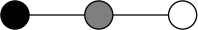
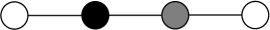
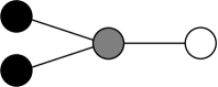
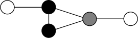
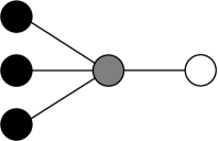
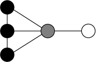
Figure 3: CSP structures up to order five

                                                                                  
                                                                                   
                                                                                   

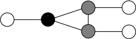
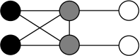
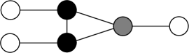
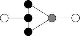
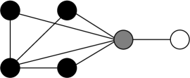
Figure 4: CSP structures in order six

6 CSP structure within the Asia-Africa-Oceania subnetwork of 1994 metal manufactures trade

The approach developed in previous sections provides a formal definition and a criterion for the systematic classification of core-semiperiphery-periphery structures in networks. In order to identify such structures in real problems, we need to develop additional results based on positional analyses allowing one to assign systematically vertices to clusters and to evaluate the extent to which the quotient network fits a CSP structure. This task, in its broad generality, exceeds the scope of the present paper and will be the object of future research. However, we discuss below a roadmap for this research by examining a given subnetwork of the network of miscellaneous imports of metal manufactures between 80 countries in 1994. These data, coming from world trade statistics, have been previously addressed in [19] along the lines discussed in the original work of Wallerstein [37]. This data set is freely available on the web (cf. [19]).

Since the results in this section have illustrative purposes and in order to simplify the discussion we restrict the attention to a subnetwork of the abovementioned network, namely the one defined by the countries from Asia, Africa and Oceania for which data are available in the original dataset. Note that the large amount of exports of high-technology products from East Asian countries makes this analysis relevant, looking in particular for their relation patterns with developing and least-developed countries from Africa, Oceania and other regions of Asia. In our model, every edge in the network is weighted with the total amount of trade between the two countries (that is, we add imports and exports). To reduce dimensionality we remove edges in which this amount does not reach 10M (10 million) USD or links involving countries whose total amount of trade does not reach 25M USD; note that these quantities barely represent a few parts per thousand of the total amount of trade in this network which is over 8 billion USD. Exceptions are made when such a removal renders the network disconnected: for the involved countries we then retain the edge displaying the highest amount of trade with any of their commercial neighbors. This yields a connected network with 29 nodes and 69 edges (data are displayed on the Appendix).

In order to examine the presence of CSP structures in this network, as well as the eventual reduction of twin substructures, we use two different criteria to cluster vertices. The first one is very elementary and just uses a threshold in the volume of trade between pairs of countries: we use this basic approach to provide simple examples of CSP structures and twin subgraphs. The second criterion is more elaborate: in order to identify clusters we combine the amount of trade between countries, as above, with a dissimilarity measure capturing similar relation patterns. This will result in a refinement of the CSP structures which arise under the first clustering criterion. Details are given below.

As indicated above, let us first cluster the different countries using the connected components of the graph which results from removing edges below a given trade threshold. Let us for instance consider pairs of countries exchanging at least 75M USD. This yields a main cluster defined by 11 countries, namely China, Hong Kong, Japan, Thailand, Korea (to be referred in the sequel as East Asian countries), together with Malaysia, Singapore, Indonesia, the Philippines (Southeast Asia), and Australia and New Zealand (both countries being jointly referred to as Australasia). This cluster comprises more than 7.7 billion USD trade, that is, more than 95% of the total amount of trade in the network. None of the remaining countries reaches the above threshold with any neighbor, so that each one of the other clusters is identified with a single country.

With this clustering, the quotient graph displays 3 countries (Algeria, South Africa, and India) which are adjacent to the main cluster and to 5 countries with degree one (Tunisia (Algeria), Israel, Mauritius, Reunion (South Africa), and Oman (India), respectively). There are 10 countries with degree one which are adjacent to the main cluster (Pakistan, Bangladesh, Egypt, Jordan, Kuwait, Morocco, Madagascar, Seychelles, Sri Lanka and Fiji). This quotient network is displayed in Figure 5(a); we explicitly label the vertices corresponding to Algeria, South Africa and India for better clarity.

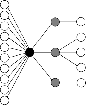
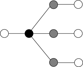
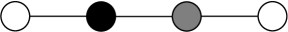
Figure 5: Clustering with threshold 75M USD: (a) CSP network; (b) Reduction of false twin vertices; (c) CSP structure.

This quotient graph admits a classification of all the clusters either as a core, semiperiphery or periphery, according to the criteria given in Definition 3. The core is composed of the East and Southeast Asian countries together with Australia and New Zealand, whereas the semiperiphery is composed of three countries (Algeria, South Africa, and India), and the fifteen countries with degree one define the periphery. Among the latter, the three ones adjacent to South Africa are false twins (we use Israel as their representative) and, analogously, the ten countries with degree one attached to the core are false twins as well (with Pakistan as the representative of this class). After identifying false twin vertices, the resulting graph is displayed in Figure 5(b). In turn, this figure clearly displays three subgraphs which are F-twins, namely, the semiperiphery-periphery pairs defined by Algeria and Tunisia, South Africa and Israel, and India and Oman, respectively. After identifying these three subgraphs (with the pair South Africa-Israel being chosen as the representative of this relation pattern), the resulting CSP structure is depicted in Figure 5(c) (it has four vertices and can be also found in Figure 3). We emphasize that the F-twin notion makes it possible to capture the elementary pattern displayed by the three semiperiphery-periphery pairs mentioned above.

Another pattern arises if we raise the threshold to cluster countries say to 125M USD. Since now neither Australia nor New Zealand trades such an amount with any Asian country, but they do with each other, they turn to define a cluster by themselves (Australasia in the sequel), independently of the East and Southeast Asian countries which are still joined together into a big cluster, trading more than 7 billion USD. The latter still meets the requirement defining a core in Definition 3, but the Australasian cluster does not, since it does not satisfy the eccentricity-two criterion (e.g. its distance to Israel is three). Australasia may by contrast be classified as a semiperiphery: note that Fiji is now attached to the Australasian cluster. The new quotient graph is displayed in Figure 6(a). As before, we depict in Figure 6(b) and (c), respectively, the network without false twin vertices and the CSP structure which finally results from removing F-twin structures (now only the Algeria-Tunisia and South Africa-Israel pairs).

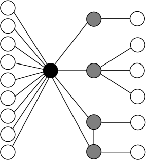
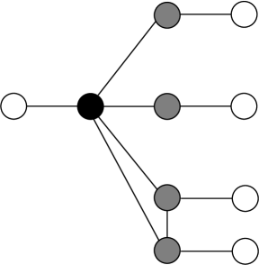
Figure 6: Clustering with threshold 125M USD: (a) CSP network; (b) Reduction of false twin vertices; (c) CSP structure.

As indicated earlier, the clustering criterion above already paves the way to illustrate some relation patterns; in a deeper analysis, however, it displays a severe limitation. Clustering countries according to their amount of trade works well for (eventually defined) core clusters, and also for some semiperipheries. But it does not accommodate the identification of semiperiphery countries which, not trading a significant amount between themselves, display however a similar (or even identical) connection pattern to the rest of the network. To incorporate this, the criterion above should be combined with a similarity (or dissimilarity) measure identifying countries with similar relation patterns.

To illustrate this idea we first raise the trade threshold above to 500M USD. This yields a smaller cluster defined by the five East Asian countries (trading more than 4.6 billion USD among themselves). Second, since we are dealing with a weighted network we define a dissimilarity criterion as follows: for each country we label each one of its incident edges with the percentage of trade that it carries, computed over the country’s total amount of trade. This percentage is zero for absent edges, that is, for pairs of countries not adjacent to each other. Denoting this percentage by $w_{ij}$ for the edge connecting vertices $i$ and $j$, the dissimilarity measure for countries $i$, $j$ is then defined as

$$\delta_{ij}=\sum_{i\neq k\neq j}|w_{ik}-w_{jk}|.$$

This means that two countries which have exactly the same connection pattern to the rest of the network have a dissimilarity measure close to zero (not exactly zero, in most cases, because even if the connections are the same the percentages will typically be different); on the contrary, if $i$ and $j$ are not adjacent and do not have any neighbor in common then the dissimilarity measure reaches the maximum value $\delta_{ij}=2$.

Ignoring peripheries, we may now define new clusters (that is, besides the main one above) in terms of this dissimilarity measure: for instance, we may join together a set of countries into a single cluster if the dissimilarities of all pairs within this set do not reach a threshold of 1.0. Two non-trivial clusters arise this way: the four Southeast Asian countries are joined into a single cluster (the six dissimilarities range from 0.33 (Malaysia-Singapore) to 0.95 (Singapore-Philippines); the total internal trade in this cluster reaches 585M USD), and so do Australia and New Zealand (with a dissimilarity of 0.59; the trade among themselves is 168M USD). The remaining countries remain isolated. Note that none of these countries reach, in any connection, the threshold of peer-to-peer trade of 500M USD defined above.

The quotient graph which results from this new clustering is displayed in Figure 7(a); now Sri Lanka is not adjacent to the core but to the Southeast Asian cluster, via Singapore. As already depicted in this figure, the five East Asian countries qualify again as a core, whereas the other clusters do not because of the eccentricity criterion. The reductions of false twin vertices and of F-twin pairs yielding a CSP structure can be found in Figure 7(b)-(c).

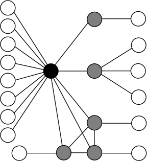
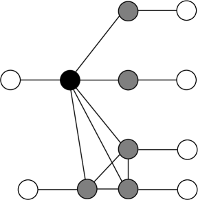
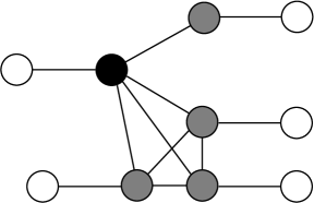
Figure 7: Adding a dissimilarity measure: (a) CSP network; (b) Reduction of false twin vertices; (c) CSP structure.

Finally, in order to further illustrate the eventual presence of other F-twin substructures, let us ignore in Figure 7(c) the edge connecting India and Australasia: among the three semiperipheries at the bottom of this figure, this is clearly the one carrying less trade (20,2M USD, whereas Southeast Asia trades 47,9M with India and over 177M with Australasia). The resulting network is depicted in Figure 8(a). Note that now the Australasia-Fiji and India-Oman pairs become F-twins; they are isomorphic, disjoint and non-adjacent, and the connection pattern to the remainder of the network is the same (both Australasia and India are connected to the core and to Southeast Asia). We can therefore reduce this new relation pattern and the resulting structure is displayed in Figure 8(b). Worth clarifying is that the Australasia-Fiji pair now stands as the representative of this pattern, which is also met by the India-Oman pair.

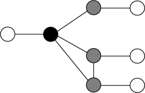
Figure 8: (a) The removal of the Australasia-India edge yields a new pair of F-twin subgraphs; (b) Resulting CSP structure.

As indicated earlier in this section, the network here analyzed is intended to illustrate the lines along which the results presented in this paper can be applied to real problems. Future study should provide a systematic analysis of clustering criteria in this context; these criteria should combine density and similarity measures. In a second step, quality measures defining the extent to which the nodes in the quotient (clustered) graph may be classified either as cores, semiperipheries or peripheries would indicate to what degree the network fits a CSP structure. When a CSP structure is actually met, the twin notions here introduced make it possible to reduce identical substructures, capturing the relation patterns depicted in the network.

The example here considered suggests that the roadmap above is a promising one. Note that the threshold parameters within the aforementioned clustering criteria (involving e.g. the amount of trade or the degree of dissimilarity between countries) has allowed for a progressive refinement of the clusters, providing gradually more detailed information about the network structure. Indeed, the (say) giant core in Figure 5(b) yields two clusters in Figure 6(b), namely East/Southeast Asia and Australasia; in turn, the East-Southeast Asian core is split in two in Figure 7(b). Accordingly, the corresponding CSP structures in Figures 5(c), 6(c) and 7(c) (with four, eight and ten nodes, respectively) gradually display more detailed information about the network structure. The network example here considered also shows how different twin structures may be identified and reduced. These include not only twin vertices but different semiperiphery-periphery patterns: compare e.g. in Figure 8(a) the Algeria-Tunisia and South Africa-Israel pairs, on the one hand, and India-Oman and Australasia-Fiji, on the other. Naturally, more complicated semiperiphery-periphery patterns would arise in larger networks.

7 Concluding remarks

Many problems related to twin subgraphs and to core-semiperiphery-periphery structures remain open for future study. We compile here some of them. First, the T-twin and F-twin notions for subgraphs introduced in Sections 3 and 4 have for sure a connection to automorphic and orbital equivalences, much as twin vertices arise in situations in which a transposition yields a graph automorphism. Note in this regard that, for vertices, the true and false twin notions accommodate all possible cases of structurally equivalent vertices, but for higher order subgraphs other twin notions besides T-twins and F-twins might be considered (for this reason we avoid using the “true” and “false” labels for our T-twin and F-twin notions, since the former labels seem to cover exhaustively all possible cases). The classification of twin structures partially addressed in subsection 3.3 also seems to have several potential extensions, in particular connected to the interrelations between the classification of different families of twin subgraphs.

Concerning the results considered in Section 5, it would be interesting to examine systematically to what extent the set of actors (countries, companies, etc.) in real social or economic networks can be clustered in a way that matches some of the structures displayed in subsection 5.4 after a suitable reduction of twin patterns: the example discussed in Section 6 suggests a plan for future research in this direction. Motivated by the enumeration of CSP structures (cf. subsection 5.3), several enumeration problems arise in connection to the absence of twin substructures in graphs: specifically, it would of interest to get a general enumeration formula for graphs without true twin vertices (or equivalently, in light of Theorem 2, for graphs without false twin vertices), and also for graphs without any kind of T-twin (or, analogously, F-twin) subgraphs. Closely related are the problems of enumerating graphs without any kind of twin vertices, or without any kind of twin subgraphs. It also seems to be worth studying other (say, layered) structures emanating from greater parameter values in Definition 3, that is, accommodating core eccentricities greater than two and/or periphery degrees greater than one. All these topics are in the scope of future research.

Appendix: The Asia-Africa-Oceania metal manufactures network

Table 3: Asia-Africa-Oceania metal manufactures trade in 1994 (from [19])

Country #1	Country #2	Trade (thoushands of USD)
China	Hong Kong	1482824
Japan	Thailand	894820
Japan	Korea	880295
China	Japan	630342
Malaysia	Singapore	484350
Japan	Malaysia	453463
Japan	Singapore	380454
Hong Kong	Japan	351919
Indonesia	Japan	200451
China	Korea	181392
Australia	New Zealand	168680
Japan	Philippines	138348
China	Singapore	135616
Japan	Australia	115283
Hong Kong	Singapore	110574
Singapore	Thailand	107720
China	Australia	90620
Australia	Indonesia	72387
Korea	Hong Kong	65315
Australia	Singapore	62392
Korea	Thailand	56160
Korea	Singapore	50098
Korea	Australia	45517
China	Thailand	44387
Australia	Malaysia	43068
Korea	Indonesia	41827
Indonesia	Malaysia	40291
China	Malaysia	39617
Singapore	Indonesia	39206
Malaysia	Thailand	37963
China	Indonesia	32817
India	Singapore	32130
Korea	Malaysia	31255
Japan	India	27655
Japan	South Africa	24555

References

- [1] M. O. Albertson, J. Pach and M. E. Young, Disjoint homometric sets in graphs, Ars Mathematica Combinatorica 4 (2011) 1-4.
- [2] N. Alon and B. Bollobás, Graphs with a small number of distinct induced subgraphs, Discrete Mathematics 75 (1989) 23-30.
- [3] M. Axenovich and L. Özkahya, On homometric sets in graphs, Electronic Notes in Discrete Mathematics 38 (2011) 83-86.
- [4] H.-J. Bandelt and H. M. Mulder, Distance-hereditary graphs, J. Combinatorial Theory B 41 (1986) 182-208.
- [5] B. Bollobás, Modern Graph Theory, Springer-Verlag, 1998.
- [6] J. A. Bondy and U. S. R. Murty, Graph Theory, Springer, 2008.
- [7] S. P. Borgatti and M. G. Everett, Regular equivalence: General Theory, J. Math. Sociology 19 (1994) 29-52.
- [8] S. P. Borgatti and M. G. Everett, Models of core/periphery structures, Social Networks 21 (1999) 375-395.
- [9] S. P. Borgatti, M. G. Everett and J. C. Johnson, Analyzing Social Networks, SAGE, 2013.
- [10] U. Brandes and T. Erlebach (eds.), Network Analysis. Methodological Foundations, Springer, 2005.
- [11] M. Burlet and J. P. Uhry, Parity graphs, in C. Berge and V. Chvátal (eds.), Topics on Perfect Graphs, Annals Discr. Mathematics, 21 (1984) 253-277.
- [12] I. Charon, I. Honkala, O. Hudry and A. Lobstein, Structural properties of twin-free graphs, The Electronic J. of Combinatorics 14 (2007) #R16.
- [13] G. Chartrand, L. Hansen, R. Rashidi, C. Chase and N. Sherwani, Distance in stratified graphs, Czechoslovak Mathematical Journal 50 (2000), 35-46.
- [14] C. Chase-Dunn, The effects of international economic dependence on development and inequality: A cross-national study, American Sociological Review 40 (1975) 720-738.
- [15] F. R. K. Chung, P. Erdős and R. L. Graham, Minimal decompositions of graphs into mutually isomorphic subgraphs, Combinatorica 1 (1981) 13-24.
- [16] P. Csermely, A. London, L.-Y. Wu and B. Uzzi, Structure and dynamics of core/periphery networks, J. Complex Networks 1 (2013) 93-123.
- [17] M. R. da Silva, H. Ma and A.-P. Zeng, Centrality, network capacity, and modularity as parameters to analyze the core-periphery structure in metabolic networks, Proc. IEEE 96 (2008) 1411-1420.
- [18] F. Della Rossa, F. Dercole and C. Piccardi, Profiling core-periphery network structure by random walkers, Sci. Reports 3 (2013) 1467.
- [19] W. de Nooy, A. Mrvar and V. Batagelj, Exploratory Social Network Analysis with Pajek, Cambridge Univ. Press, 2011.
- [20] R. Diestel, Graph Theory, Springer-Verlag, 2000.
- [21] P. Erdős and A. Hajnal, On the number of distinct induced subgraphs of a graph, Annals of Discrete Mathematics 43 (1989) 145-154.
- [22] J. Gamble, H. Chintakunta, A. Wilkerson and H. Krim, Node dominance: Revealing community and core-periphery structure in social networks, IEEE Trans. on Signal and Information Processing over Networks 2 (2016) 186-199.
- [23] F. Harary, Graph Theory, Addison-Wesley, 1969.
- [24] C. Hernando, M. Mora, I. M. Pelayo, C. Seara and D. R. Wood, Extremal graph theory for metric dimension and diameter, Electronic Notes in Discrete Mathematics 29 (2007) 339-343.
- [25] C. Hernando, M. Mora and I. M. Pelayo, On the partition dimension and the twin number of a graph, ArXiV, 2016.
- [26] C. A. Hidalgo, B. Klinger, A.-L. Barabási and R. Hausmann, The product space conditions the development of nations, Science 317 (2007) 482-487.
- [27] P. Holme, Core-periphery organization of complex networks, Phys. Rev. E 72 (2005) 046111.
- [28] I. Honkala, O. Hudry and A. Lobstein, On the number of optimal identifying codes in a twin-free graph, Discrete Applied Mathematics 180 (2015) 111-119.
- [29] E. Korach, U. N. Peled and U. Rotics, Equistable distance-hereditary graphs, Discrete Applied Mathematics 156 (2008) 462-477.
- [30] E. Lazega, Synchronization costs in the organizational society: Intermediary relational infrastructures in the dynamics of multilevel networks, in E. Lazega and T. Snijders (eds.), Multilevel Network Analysis for the Social Sciences, pp. 47-77, Springer, 2016.
- [31] C. Lee, P.-S. Loh and B. Sudakov, Self-similarity of graphs, SIAM Journal on Discrete Mathematics 27 (2013) 959-972
- [32] R. J. Nemeth and D. A. Smith, International trade and world-system structure: A multiple network analysis, Review 8 (1985) 517-560.
- [33] M. E. J. Newman, Networks, Oxford Univ. Press, 2010.
- [34] M. P. Rombach, M. A. Porter, J. H. Fowler and P. J. Mucha, Core-periphery structure in networks, SIAM J. Appl. Math. 74 (2014) 167-190.
- [35] J. Rosenblatt and P. D. Seymour, The structure of homometric sets, SIAM J. Algebraic Discrete Methods 3 (1982) 343-350.
- [36] D. Snyder and E. L. Kick, Structural position in the world system and economic growth, 1955-1970: A multiple-network analysis of transnational interactions, American Journal of Sociology 84 (1979) 1096-1126.
- [37] I. Wallerstein, The Modern World-System: Capitalist Agriculture and the Origins of the European World-Economy in the Sixteenth Century, Academic Press, 1974.
- [38] X. Zhang, T. Martin and M. E. J. Newman, Identification of core-periphery structure in networks, Phys. Rev. E 91 (2015) 032803.