Principal component analysis and sparse polynomial chaos expansions for global sensitivity analysis and model calibration: application to urban drainage simulation

Abstract

This paper presents an efficient surrogate modeling strategy for the uncertainty quantification and Bayesian calibration of a hydrological model. In particular, a process-based dynamical urban drainage simulator that predicts the discharge from a catchment area during a precipitation event is considered. The goal is to perform a global sensitivity analysis and to identify the unknown model parameters as well as the measurement and prediction errors. These objectives can only be achieved by cheapening the incurred computational costs, that is, lowering the number of necessary model runs. With this in mind, a regularity-exploiting metamodeling technique is proposed that enables fast uncertainty quantification. Principal component analysis is used for output dimensionality reduction and sparse polynomial chaos expansions are used for the emulation of the reduced outputs. Sensitivity measures such as the Sobol indices are obtained directly from the expansion coefficients. Bayesian inference via Markov chain Monte Carlo posterior sampling is drastically accelerated.

The quantification of uncertainty has become an integral aspect of computational science and engineering in the last two decades [1, 2]. Algorithmic advances on the one hand and hardware improvements on the other hand allow for an increasingly detailed simulation of complex systems. That the underlying models are hardly perfect and the model parameters are barely known with certainty prompts scientist and engineers to conduct an end-to-end analysis of the encountered errors. This process, for which one commonly relies on probability theory, is known as uncertainty quantification (UQ).

Nowadays, the study and possible reduction of uncertainties are important to virtually all engineering fields. Some UQ applications can be found in [3, 4] for instance. Due to the prevalence of uncertainties in the mathematical modeling and numerical simulation of environmental and water systems, UQ is of special importance to hydrological disciplines [5, 6]. Recent reviews of UQ in the latter context are for example found in [7, 8, 9].

The overall goal of UQ is the fair assessment and subsequent improvement of the accuracy of predictive models. This provides the basis for model-assisted decision making [10, 11] and real-time control [12], which ultimately supports the effective management of engineered and environmental systems. In this sense, the adequate representation, thorough analysis and treatment of uncertainty is an ambitious project whose realization typically involves a variety of sub-tasks. These standard UQ tasks encompass expert elicitation [13, 14], uncertainty propagation [15, 16], sensitivity analysis [17, 18] and Bayesian analysis [19, 20].

In forward propagation, one starts by assigning a probability distribution to the uncertain parameters of a predictive model. Afterwards, the goal is to determine the corresponding distribution of the model response [21, 22]. While the input distribution reflects the degree as to which one does not know the parameter values precisely, the output distribution quantifies the lack of confidence that we must have in the model predictions. A standard method to perform uncertainty forward propagation is Monte Carlo (MC) simulation [23]. Here, one draws independent samples from the input distribution and computes the corresponding model responses. Thereupon, the statistical moments and a histogram-based representation of the output distribution can be obtained. MC sampling is very robust and rests on mild assumptions, yet it is very expensive and suffers from a slow convergence rate.

The study of how important the various input parameters are with respect to the model response is called sensitivity analysis [24, 25]. There are certainly different possibilities of defining and analyzing sensitivity measures. In a global variance-based analysis one compares and ranks the input variables according to their contribution to the total response variance [26, 27]. This does not only provide valuable insight into the input-output relationship established by the model, it also allows one to restrict the attention to the most influential parameters and to allocate the available resources accordingly. Though, the practical computation of global sensitivity indices, e.g. in a MC sampling framework, is usually expensive because it requires a moderate to high number of model evaluations.

Bayesian inference is a probabilistic framework for statistical inference and uncertainty reduction [28, 29]. The initial uncertainty of the parameters, before the data have been realized or at least before they are analyzed, is formulated as the prior probability distribution. A conditional statistical model of the observables given values of the unknown parameters, which for the actual data gives rise to the likelihood function, is constructed. Eventually, the posterior distribution ensues from Bayes’ law. This is a distribution of the unknown parameters conditioned on the acquired observations, i.e. it represents the new state of knowledge and reduced uncertainty after the information contained in the data has been processed. The mean or the mode of the posterior are often taken as point estimates of the parameters, whereas the spread of the posterior can be regarded as a measure of the statistical estimation uncertainty. Bayesian inference does not only establish a consistent foundation for parameter estimation and inverse modeling, it can also provide solid answers to the delicate question of model discrepancy [30, 31]. Moreover, model evidences can be judged, which in turn enables model comparison, selection and averaging [32, 33].

The chief task in Bayesian inference is the computation of the posterior distribution. Sampling-based approaches such as Markov chain Monte Carlo (MCMC) [34, 35] are by far the most widespread techniques for computational Bayesian inference. Here, the idea is to construct an ergodic Markov chain that exhibits the posterior as the stationary distribution. The posterior can be sampled that way and all relevant conditional expectation values can be estimated. Unfortunately, due to the sample autocorrelation, MCMC is less efficient than standard MC simulation with independent samples. Therefore, the procedure usually calls for a large number of algorithmic iterations and evaluations of the forward model. This causes an excessive computational cost which easily exceeds the available budget. A plethora of advanced sampling methods exists, e.g. gradient-driven updating schemes with auxiliary variables [36, 37] or population-based samplers resting on a tempering schedule [38, 39]. Beyond that, there are some fundamentally different alternatives to MCMC sampling, e.g. based on variational strategies [40, 41], optimal transportation theory [42, 43] or spectral likelihood expansions [44]. But despite these efforts, Bayesian model calibration remains a costly endeavor. Additional costs are even occasioned when the relative evidences of various competing models have to be assessed [45, 46].

Following these remarks, one has to recognize that UQ tasks are extremely computing-intensive, especially for hydrological applications where the underlying processes are often studied by reference to nonlinear and highly parametrized models. This brings about long computation times and complicates all rigorous uncertainty analyses that require many model runs, i.e. forward propagation, sensitivity analysis and statistical inference. In the worst case, hydrologists would be precluded from carrying out important activities, e.g. the intelligent operation of urban infrastructure through state-of-the-art model-based predictive control methods could be completely prohibited thereby. It is also conceivable that, because the evidence-grounded inference of physical parameters is rendered impossible, parameter values have to be chosen in an ad-hoc fashion. This could lead to questionable predictions and results.

If one does not want to resort to oversimplified models or to discard some system analyses and control strategies, one may consider employing a fast metamodel or surrogate model [47, 48]. This possibility has received much attention lately. A surrogate model is constructed so as to emulate the input-output relation of the original simulator, i.e. it is a function approximation. The most important behavioral characteristics should be reproduced and the emulator must be cheap to evaluate. Very often, this goal can be achieved with Gaussian process regression [49, 50] or a polynomial chaos expansion (PCE) [51, 52]. The former is an interpolation routine that is predicated on the conditioning of a Gaussian process prior for the simulator. The latter approach bears on a basis decomposition of the response random variable into orthogonal polynomials in the input variables. In a non-intrusive manner, a representative sample of model inputs and the associated model responses can be used to train either of the mentioned emulators.

After a metamodel is constructed, it can replace the simulator in any of the discussed UQ analyses, e.g. in MC simulation for uncertainty forward propagation. It turns out that UQ can be significantly accelerated that way. The reason is that metamodeling allows one to exploit structures and regularity properties of the forward problem. In Gaussian process regression one can incorporate prior knowledge about the functional relationship through the mean and covariance function of the Gaussian process. Physical understanding and expectations regarding the smoothness can be integrated hereby. Polynomial expansions rest on the assumption that the model response can be represented well in the global basis. They allow for finding and utilizing compressibility (i.e. the spectrum of the coefficients decays fast) and sparsity (i.e. only a small fraction of the terms contribute significantly).

Of course, in the construction of a sufficiently accurate and fast emulator one may also face problems. The curse of dimensionality stands for a number of phenomena that form obstacles to the study of high-dimensional systems. In the first instance, this relates to the high-dimensionality of the input space, which impedes UQ analyses in general. For the computation of PCE-based metamodels in particular, as mentioned above, one can alleviate the curse by seeking sparsity with the aid of regularized regression [53, 54, 55] and its Bayesian variants [56, 57, 58]. Another problem, that very often arises in the simulation of time-dependent hydrological processes, is related to high-dimensional model outputs. In order to understand and eventually approximate the functional relationship between the uncertain hydrological parameters and the corresponding predictions at successive time instants, the latter have to be seen as different output variables. Since current metamodeling techniques treat each of these scalar outputs separately, and long time series may comprise some ten thousand points, this might become a critical problem in hydrological applications.

Motivated by the preceding discussion, the goal of this paper is the development of efficient surrogate models in the context of dynamical rainfall-runoff simulation, and the subsequent facilitation of the sensitivity analysis and Bayesian calibration of a slow process-based urban water simulator. The following regularity-exploiting strategy is pursued to that end. First, principal component analysis is used for reducing the dimensionality of the combined model output, that comprises the predicted runoffs at various time instants. This allows us to exploit the fact that discharge is a rather well-structured phenomenon, i.e. as function of the random inputs, the discharge at adjacent times is highly correlated. Second, the low number of principal components obtained this way is metamodeled through sparse polynomial expansions. Thereby we utilize the sparsity found in the basis decomposition of the hydrological model. Principal component analysis and polynomial chaos expansions, each taken by itself, are well-established tools. Their synergy potential, however, has attracted little to no attention so far.

Another novelty is that, third, we introduce a new estimator of time-variant variance-based sensitivity measures in connection with the chosen emulation approach. We show that one can obtain the sensitivities of the original simulator outputs with respect to the uncertain inputs from the expansion coefficients of the principal components. Last, a comprehensive Bayesian analysis of the parametric uncertainties and modeling errors is conducted. An explicitly parametrized term is introduced that represents the systematic model discrepancy as a function of time. This term acts additively on the model predictions and it can be inferred together with the unknown model parameters. In order to demonstrate the proposed methods, a case study is executed that involves a drainage model of an urban catchment area in Switzerland and real experimental data. Notwithstanding that all developed methods are explained and demonstrated on the basis of this specific problem, they are more generally applicable and can be readily adapted to other water resources or environmental applications.

The remainder of the paper is organized as follows. An overview of the forward problem setup and the information available for the model calibration is provided in Section 1. The construction of the multivariate emulator by means of output dimensionality reduction and sparse polynomial chaos expansions is described in Section 2. Details on the estimation of global variance-based sensitivity measures are given in Section 3. Bayesian parameter estimation and predictive model correction are performed in Section 4. Finally it is summarized and concluded in Section 5.

1 Problem setup

In hydrology one distinguishes between physical process-based and purely data-driven modeling approaches [59, 60]. Due to complicated interactions of the relevant compartments at several spatial and temporal scales, the physics-oriented simulation of urban water systems is a peculiarly uncertainty-prone procedure [61, 62]. This motivates a thorough error and uncertainty analysis. In this paper, such an analysis is performed for a computer model which predicts the time-varying runoff from an urban drainage basin that receives precipitation, see [63] for a more detailed description. The dynamical simulation of the outflow is based on a series of rainfall intensity measurements, and it requires knowledge of model parameters such as the Gauckler–Manning roughness coefficients or the sub-catchment slopes. Unfortunately, the values of those parameters are not precisely known, i.e. they are uncertain. Moreover, even if the input parameters could be known perfectly, the predicted outputs would be still subject to inevitable model-immanent errors and discrepancies.

For the analysis and eventual reduction of the aforementioned uncertainties, we have the following pieces of information at hand. Bounds and prior distributions of the unknown hydrological parameters are established. They represent the parametric uncertainties before the data are analyzed. About six hundred measurements of the rainfall intensity during a precipitation event, observed by a single rain gauge in the catchment, and the runoff at a single outlet are available. Besides, we have the precomputed results of roughly two thousand training runs of the simulator. They were performed for the recorded rainfall data, while the uncertain parameters had taken on different values in each of those runs. Before we begin with surrogate modeling, sensitivity analysis and model calibration, this section contains a brief description of the urban drainage model under consideration and the experimental data at our disposal.

The storm water management model (SWMM) is a dynamic rainfall-runoff simulation program for urban areas [64]. It can be used to predict water levels in sewer manholes and the runoff from catchment areas during dry and wet weather. A model of the drainage basin of Adliswil, a municipality in the canton of Zürich in the northeast of Switzerland, was developed with the SWMM at the Swiss Federal Institute of Aquatic Science and Technology. In Fig. 1 a map is provided that shows the surrounding area of the size $5\,\mathrm{km}\times 3\,\mathrm{km}$. About $160\,\mathrm{ha}$ of this area, i.e. approximately ten percent, are considered in the model. As very detailed land-use information is available, the catchment is represented with approximately one hundred sub-catchments that are drained by a network consisting of five hundred pipes.

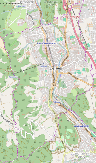
Figure 1: Adliswil, Switzerland (1:50000). From OpenStreetMap under CC BY-SA 2.0. © OpenStreetMap contributors.

All sub-catchments and sewer pipes are associated with their own set of unknown parameters. This amounts to a fairly large number of unknowns which is reduced by considering spatial averages only, i.e. physical quantities of the same type are averaged over the sub-catchments or channels. The resulting averages thus relate to the catchment as a whole. Moreover, the parameters are normalized so as to be dimensionless and to lie in between reasonable bounds. A compilation of the so-obtained scaled parameters $x_{i}\in\mathcal{D}_{x_{i}}$ for $i=1,\ldots,8$ and their bounded domains $\mathcal{D}_{x_{i}}=[\underline{x}_{i},\overline{x}_{i}]$ is presented in Table 1. Here, the lower and upper bounds are denoted as $\underline{x}_{i}$ and $\overline{x}_{i}$, respectively. The physical quantities described and their unscaled averages are also provided in the table. While the first seven parameters relate to the sub-catchments, only the last one characterizes the pipes.

Table 1: Hydrological model parameters.

$x_{i}$	$\mathcal{D}_{x_{i}}$	Physical parameter	Spatial average
$x_{1}$	$[0.5,1.1]$	Percentage of the impervious area	$36\,\mathrm{\%}$
$x_{2}$	$[0.5,1.5]$	Characteristic width of the overland flow path	$35.7\,\mathrm{m}$
$x_{3}$	$[0.5,1.5]$	Slope of the sub-catchments	$11.4\,\mathrm{\%}$
$x_{4}$	$[0.5,1.5]$	Depression storage height of the impervious area	$2\,\mathrm{mm}$
$x_{5}$	$[0.5,1.5]$	Manning roughness coefficient of the impervious area	$0.12\,\mathrm{s\cdot m^{-1/3}}$
$x_{6}$	$[0.5,1.5]$	Depression storage height of the pervious area	$2\,\mathrm{mm}$
$x_{7}$	$[0.5,1.5]$	Percentage of the impervious area without depression storage	$19.04\,\mathrm{\%}$
$x_{8}$	$[1.0,1.5]$	Manning roughness coefficient of the channels	$0.012\,\mathrm{s\cdot m^{-1/3}}$

A single $15$-hour rainfall event is considered that had occurred on May 28, 2013. Time is denoted as $t$ in the following. The experiment extends over a period with $t/120\,\mathrm{s}\in[0,600]$. Measurements of the varying rainfall intensity $I$ and the catchment outflow $Q$ are taken in regular intervals of two minutes over the full duration. For $i=0,\ldots,600$ the time instants of the observations are denoted as $t_{i}$. Both rainfall and outflow measurements were made at single locations within the drainage basin, e.g. the outflow was measured at the outlet of the system, close to the wastewater treatment plant. In Fig. 2 the available data are summarized. The observations of the rainfall intensity $I(t_{i})$ are indicated by the black dots in Fig. 2. Owing to the resolution of the measurement device, the recorded intensity takes on discrete values only. The recorded outflows $Q(t_{i})$ at the sewage treatment plant are shown in Fig. 2.

Beyond the observational data just described, the results of approximately two thousand runs of the SWMM simulator are available. These will constitute the training runs for the computation of the surrogate model in the next section. They were conducted for the rainfall data shown in Fig. 2 and uniformly distributed values of the uncertain hydrological parameters. The runtime for a single SWMM simulation amounts to approximately twenty seconds. For the sake of illustration, a hundred trajectories from these computer simulations are depicted in Fig. 2. They can be compared to the actually measured runoffs in the same plot.

The model manages to capture the main trends and characteristics of the data. However, in the time interval $t/120\,\mathrm{s}\in[150,200]$ the model systematically underpredicts the outflow. An even stronger systematic discrepancy is detected for the time span $t/120\,\mathrm{s}\in[250,500]$ during which the outflow is overpredicted. It is also noticed that the model predictions for different values of the uncertain inputs do not differ significantly, i.e. they cannot be discriminated very well by their ability to trace the data. The effect is especially obvious in the second half of the experiment with $t/120\,\mathrm{s}\in[300,600]$. Here, the mismatch between the data and the model predictions is apparently dominated by systematic errors and random noise rather than by variations of the model inputs. This motivates the study of model discrepancy as a function of time. While random noise can be at least partially attributed to uncertainties in the measurement process, the systematic errors are a consequence of the model simplifications. Especially the limitation to spatial parameter averages only, instead of a more refined representation as spatially variable fields for example, is believed to be a major factor contributing to the observed time-dependent discrepancies.

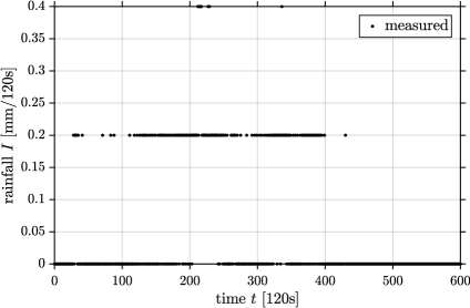
(a) Rainfall intensity.

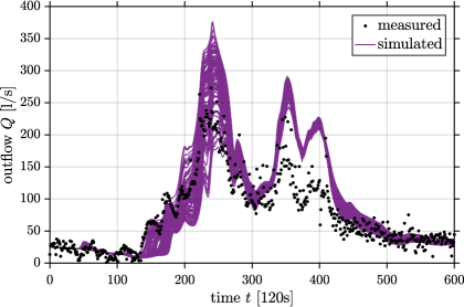
(b) Catchment outflow.

Figure 2: Available data. Observations of the time-dependent rainfall intensity are shown in Fig. 2. Their discrete values reflect the resolution of the measurement procedure. The actually measured outflows during the event can be compared against an ensemble of one hundred simulations in Fig. 2. While the simulations and measurements are in rough accordance with each other, some systematic deviations can be identified in the time interval $[150,200]$ and, more obviously, in $[250,500]$.

2 Surrogate modeling

In computing-intensive studies it has become common practice to replace an expensive-to-run simulator of the system by a cheap-to-evaluate surrogate [47, 48]. These so-called metamodels or emulators try to mimic the originally defined input-output relationship as closely as possible. Dynamic simulators can be emulated in a purely statistics-based manner, e.g. by conditioning a Gaussian process prior on the experimental design. Mechanism-based approaches try to enhance the emulation through an appropriate incorporation of the available physical understanding [65, 66]. In particular, the solution of a simplified problem is incorporated into the prior and subsequently corrected so as to emulate the full simulator. An application of this approach to the Adliswil watershed can be found in [67].

Polynomial chaos expansions [68, 69] establish an alternative to Gaussian process–based metamodels. In this context, structure-exploiting regression formulations [53, 56] do not only capitalize on the smoothness of the forward model, they also allow one to seek for and eventually benefit from sparsity in the expansions. At the same time, this promises high accuracy and good scalability with the dimensionality of the input space and the size of the training data. Examples for the use of sparse polynomial surrogates in hydrological applications are found in [70, 71] for instance.

In this section we pursue an integrated strategy that draws on both dimension reduction and polynomial metamodeling. First, the dimensionality of combined model output, which consists of all time-indexed predictions, is reduced through principal component analysis. This allows us to minimize the degree of redundancy that is inherent in the simulation of a highly structured process such as the time-variant outflow. Then, chaos expansions are computed for the main components as functions of the uncertain inputs, which allows for revealing and leveraging certain sparsity patterns of the forward model. Last, the obtained expansions are combined in order to obtain a multivariate surrogate model for the full time series of the outflow. In so doing, the regular properties of the forward problem can be fully taken advantage of. That the method is fully non-intrusive, i.e. it is solely based on precomputed input-output pairs, allows for a straightforward adaptation to other problems.

2.1 Training runs

The SWMM implementation of the catchment predicts a complete discharge time series at the system outlet close to the wastewater treatment plant throughout the precipitation event. For the given rainfall intensity record, the model only acts as a function of the uncertain input parameters listed in Table 1. Thus we gather the unknown model input parameters in a vector $\bm{x}=(x_{1},\ldots,x_{M})^{\top}$ with $M=8$. Similarly we proceed for the rainfall data $\bm{d}=(d_{0},\ldots,d_{N})^{\top}$ with $N=600$. For $i=0,\ldots,N$ we have introduced $d_{i}=I(t_{i})$ for the observed rainfall intensities at the measurement time instants $t_{i}$.

The numerical model predicts the vector $\tilde{\bm{y}}=(\tilde{y}_{0},\ldots,\tilde{y}_{N})^{\top}$ whose entries are the outflows $\tilde{y}_{i}=\tilde{Q}(t_{i})$ at the times $t_{i}$. All in all, $\tilde{\bm{y}}=\mathcal{M}(\bm{x},\bm{d})$ reflects the structure of the hydrological simulations. Since we only consider a single precipitation event and disregard errors in the rainfall data, we absorb the dependence on the rainfall into the definition of the forward model $\mathcal{M}_{\bm{d}}$ by

$$\tilde{\bm{y}}=\mathcal{M}_{\bm{d}}(\bm{x}).$$ (1)

Note that the dynamical nature of the original system is now completely captured through the pooled multivariate output structure of the model in Eq. 1.

We now switch to a probabilistic formulation, where the inputs are modeled as independent $\mathcal{D}_{x_{i}}$-valued random variables $X_{i}\sim\mathcal{U}(x_{i}\>\!|\>\!\underline{x}_{i},\overline{x}_{i})$ with uniform distributions over the intervals $[\underline{x}_{i},\overline{x}_{i}]$ for $i=1,\ldots,M$. The random vector $\bm{X}\sim\prod_{i=1}^{M}\mathcal{U}(x_{i}\>\!|\>\!\underline{x}_{i},\overline{x}_{i})$ with values in $\mathcal{D}_{x_{1}}\times\mathcal{D}_{x_{2}}\times\ldots\times\mathcal{D}_{x_{M}}$ then represents the input uncertainty. When the model $\mathcal{M}_{\bm{d}}$ is applied to the random inputs $\bm{X}$, the output uncertainty is described by the $\mathds{R}^{N+1}$-valued random vector

$$\tilde{\bm{Y}}=\mathcal{M}_{\bm{d}}(\bm{X}).$$ (2)

For later considerations, i.e. stochastic spectral expansions and variance decompositions, we will assume from now on tacitly that all components of this random response vector have a finite variance.

In order to construct a metamodel that allows us to cheaply predict to model response for arbitrary values of the inputs, in total $K=2,048$ training runs were conducted. Realizations $\bm{x}^{(k)}$ of the input variables had to be obtained for $k=1,\ldots,K$ and the corresponding realizations $\tilde{\bm{y}}^{(k)}=\mathcal{M}_{\bm{d}}(\bm{x}^{(k)})$ of Eq. 2 had to be computed. The inputs were created by Latin hypercube sampling [72] in two chunks of $1,024$ samples each. Altogether they constitute the experimental design $\mathcal{X}=(\bm{x}^{(1)},\ldots,\bm{x}^{(K)})$. The computed model responses, some of which were already shown in Fig. 2, are collected into the data matrix

$$\mathcal{Y}=\begin{pmatrix}\tilde{\bm{y}}^{{(1)}^{\top}}\\ \tilde{\bm{y}}^{{(2)}^{\top}}\\ \vdots\\ \tilde{\bm{y}}^{{(K)}^{\top}}\\ \end{pmatrix}=\begin{pmatrix}\tilde{y}_{0}^{(1)}&\tilde{y}_{1}^{(1)}&\ldots&\tilde{y}_{N}^{(1)}\\ \tilde{y}_{0}^{(2)}&\tilde{y}_{1}^{(2)}&\ldots&\tilde{y}_{N}^{(2)}\\ \vdots&\vdots&\ddots&\vdots\\ \tilde{y}_{0}^{(K)}&\tilde{y}_{1}^{(K)}&\ldots&\tilde{y}_{N}^{(K)}\\ \end{pmatrix}.$$ (3)

2.2 Principal component analysis

The coordinates of the model output with respect to a certain reference system, e.g. the canonical basis, could now be metamodeled individually. In our case, this would require to handle about six hundred different metamodels simultaneously. That is inconvenient and may even become infeasible for problems with much longer time series. Also, it involves a high degree of redundancy, i.e. the simulation outputs at contiguous times are highly correlated.

To find a remedy one can choose a basis that is qualified for purposes of dimension reduction and data compression. Here we use principal component analysis (PCA) [73] to that end. While this technique is mainly used for compressing big real-world data sets with many features, it can be similarly used for reducing the model output in the context of computer simulations [74, 75]. A discussion of the population PCA for a random vector, which is the discrete variant of the Karhunen–Loève (KL) expansion of a stochastic process [76], is found at the end of the paper in Appendix A. The empirical sample PCA is recalled in the following.

Much in the same way as the population PCA works for a random vector, i.e. an orthogonal transformation is applied such that linearly uncorrelated variables with decreasing variances are obtained, a set of observed realizations from the random vector is processed in the sample PCA. We consider the random vector $\tilde{\bm{Y}}$ that represents the model output and a number of realizations $\mathcal{Y}=(\tilde{\bm{y}}^{(1)},\ldots,\tilde{\bm{y}}^{(K)})^{\top}$ from it. Instead of the exact mean $\bm{\mu}_{\tilde{\bm{Y}}}=\mathds{E}[\tilde{\bm{Y}}]$ and covariance matrix $\bm{\Sigma}_{\tilde{\bm{Y}}}=\mathrm{Cov}[\tilde{\bm{Y}}]$, which cannot be determined exactly, one takes their empirical estimates

$$\overline{\bm{\mu}}_{\tilde{\bm{Y}}}=\frac{1}{K}\sum\limits_{k=1}^{K}\tilde{\bm{y}}^{(k)},\quad\overline{\bm{\Sigma}}_{\tilde{\bm{Y}}}=\frac{1}{K-1}\sum\limits_{k=1}^{K}(\tilde{\bm{y}}^{(k)}-\overline{\bm{\mu}}_{\tilde{\bm{Y}}})(\tilde{\bm{y}}^{(k)}-\overline{\bm{\mu}}_{\tilde{\bm{Y}}})^{\top}.$$ (4)

For $i=0,\ldots,N$ the eigenvectors $\overline{\bm{\phi}}_{i}$ and eigenvalues $\overline{\lambda}_{i}$ of the empirical covariance fulfill $\overline{\bm{\Sigma}}_{\tilde{\bm{Y}}}\overline{\bm{\phi}}_{i}=\overline{\lambda}_{i}\overline{\bm{\phi}}_{i}$. The eigenvalues are arranged in the descending order $\overline{\lambda}_{0}\geq\overline{\lambda}_{1}\geq\ldots\geq\overline{\lambda}_{N}$.

Then one finds the smallest $N^{\prime}\leq N$ for which the proportion $\sum_{i=0}^{N^{\prime}}\overline{\lambda}_{i}/\sum_{i=0}^{N}\overline{\lambda}_{i}$ of the total empirical variance is larger or at least equal than a prespecified threshold. The matrix $\overline{\bm{\Phi}}_{N^{\prime}}=(\overline{\bm{\phi}}_{0},\overline{\bm{\phi}}_{1},\ldots,\overline{\bm{\phi}}_{N^{\prime}})$ is composed and for $k=1,\ldots,K$ one defines

$$\tilde{\bm{z}}^{(k)}=\overline{\bm{\Phi}}_{N^{\prime}}^{\top}(\tilde{\bm{y}}^{(k)}-\overline{\bm{\mu}}_{\tilde{\bm{Y}}}).$$ (5)

This is the reduced PCA representation of $\tilde{\bm{y}}^{(k)}$ in terms of the empirical principal components $\tilde{z}_{i}^{(k)}=\overline{\bm{\phi}}_{i}^{\top}(\tilde{\bm{y}}^{(k)}-\overline{\bm{\mu}}_{\tilde{\bm{Y}}})$ for $i=0,\ldots,N^{\prime}$. The data set is compressed while retaining most of the total variation by

$$\mathcal{Z}=\begin{pmatrix}\tilde{\bm{z}}^{{(1)}^{\top}}\\ \tilde{\bm{z}}^{{(2)}^{\top}}\\ \vdots\\ \tilde{\bm{z}}^{{(K)}^{\top}}\\ \end{pmatrix}=\begin{pmatrix}\tilde{z}_{0}^{(1)}&\tilde{z}_{1}^{(1)}&\ldots&\tilde{z}_{N^{\prime}}^{(1)}\\ \tilde{z}_{0}^{(2)}&\tilde{z}_{1}^{(2)}&\ldots&\tilde{z}_{N^{\prime}}^{(2)}\\ \vdots&\vdots&\ddots&\vdots\\ \tilde{z}_{0}^{(K)}&\tilde{z}_{1}^{(K)}&\ldots&\tilde{z}_{N^{\prime}}^{(K)}\\ \end{pmatrix}.$$ (6)

The compression of the data is lossy, but one can reconstruct the originally observed samples for $k=1,\ldots,K$ approximately as

$$\tilde{\bm{y}}^{(k)}\approx\overline{\bm{\mu}}_{\tilde{\bm{Y}}}+\overline{\bm{\Phi}}_{N^{\prime}}\tilde{\bm{z}}^{(k)}=\overline{\bm{\mu}}_{\tilde{\bm{Y}}}+\sum\limits_{i=0}^{N^{\prime}}\tilde{z}_{i}^{(k)}\overline{\bm{\phi}}_{i}.$$ (7)

Now we perform PCA to our sample of SWMM simulator responses $\mathcal{Y}=(\tilde{\bm{y}}^{(1)},\ldots,\tilde{\bm{y}}^{(K)})^{\top}$. Using $N^{\prime}+1=9$ principal components captures $99\,\mathrm{\%}$ of the total variance of the signal. Hundred realizations contained in the compressed data set $\mathcal{Z}=(\tilde{\bm{z}}^{(1)},\ldots,\tilde{\bm{z}}^{(K)})^{\top}$ are visualized in the parallel coordinate plot in Fig. 3. These are the empirical principal components of the sample of training runs that were already shown in Fig. 2. It can be seen that the main components are centered around zero and ordered according to their individual contribution to the total variance.

Figure 3: Principal component analysis. The simulated outflows are compressed into the first eight principal components. This is visualized for the hundred realizations that were already depicted in Fig. 2.

2.3 Polynomial chaos expansions

In order to construct a surrogate model of the $N+1$ components of the forward model response $\tilde{\bm{Y}}$ as a function of the unknown parameters $\bm{X}$, we now only have to metamodel the first principal components $\tilde{z}_{p}(\bm{X})=\tilde{Z}_{p}$ for $p=0,\ldots,N^{\prime}$ in Eq. 35. This can be done through PCEs [51, 52]. Here, one starts with a family of polynomials $\{\Psi_{\alpha_{i}}^{(i)}(X_{i})\}_{\alpha_{i}\in\mathds{N}}$ in a single input variable $X_{i}\in\mathcal{D}_{x_{i}}$ that is indexed by the polynomial degree $\alpha_{i}\in\mathds{N}$. The polynomials are assumed to be orthonormal in the sense that $\mathds{E}[\Psi^{(i)}_{\alpha_{i}}(X_{i})\Psi^{(i)}_{\beta_{i}}(X_{i})]=\delta_{\alpha_{i}\beta_{i}}$.

This way, a couple of well-known probability distributions are associated with certain families of orthogonal polynomials [77]. A list of four univariate distributions, their supports and the corresponding polynomials is provided in Table 2. The first six members of the Legendre polynomials $\{\Psi_{\alpha}(x)\}_{\alpha=0}^{5}$ in a single variable $x\in[-1,1]$, that are orthogonal with respect to the uniform distribution $\pi(x)=\mathcal{U}(x\>\!|\>\!-1,1)$, are shown in Fig. 4. When the random model parameters do not have a standard form, i.e. they do not follow a classical distribution, one has to transform to standardized variables that follow such a distribution. As an alternative, one can numerically construct a sequence of polynomials that are orthogonal with respect to an arbitrary non-standard input distribution [78].

Table 2: Orthogonal polynomials.

Distribution	Support	Polynomials
Gaussian	$(-\infty,\infty)$	Hermite
Uniform	$[-1,1]$	Legendre
Beta	$[-1,1]$	Jacobi
Gamma	$[0,\infty)$	Laguerre

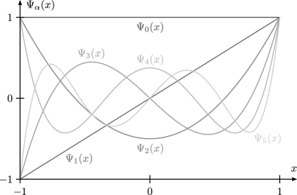
Figure 4: Legendre polynomials.

Assuming that the input density factorizes as $\pi(\bm{x})=\pi_{1}(x_{1})\ldots\pi_{M}(x_{M})$, one can construct a family $\{\Psi_{\bm{\alpha}}(\bm{X})\}_{\bm{\alpha}\in\mathds{N}^{M}}$ of multivariate polynomials by $\Psi_{\bm{\alpha}}(\bm{X})=\Psi^{(1)}_{\alpha_{1}}(X_{1})\ldots\Psi^{(M)}_{\alpha_{M}}(X_{M})$. The multi-index $\bm{\alpha}=(\alpha_{1},\ldots,\alpha_{M})\in\mathds{N}^{M}$ characterizes the polynomials. This basis can be used to expand the random variables $\tilde{z}_{p}(\bm{X})$ for $p=0,\ldots,N^{\prime}$ with finite variance as

$$\tilde{z}_{p}(\bm{X})=\sum\limits_{\bm{\alpha}\in\mathds{N}^{M}}a_{p,\bm{\alpha}}\Psi_{\bm{\alpha}}(\bm{X}).$$ (8)

Here, the set of coefficients $\{a_{p,\bm{\alpha}}\}_{\bm{\alpha}\in\mathds{N}^{M}}$ is defined through the orthogonal projections $a_{p,\bm{\alpha}}=\mathds{E}[\tilde{z}_{p}(\bm{X})\Psi_{\bm{\alpha}}(\bm{X})]$. The series in Eq. 8 has to be truncated in practice. This can be done by limiting the total polynomial degree $\lVert\bm{\alpha}\rVert_{1}=\sum_{p=1}^{M}\lvert\alpha_{p}\rvert\leq\gamma$ to a certain $\gamma\in\mathds{N}$. Only terms with $\bm{\alpha}\in\mathcal{A}_{\gamma}=\{\bm{\beta}\in\mathds{N}^{M}\colon\lVert\bm{\beta}\rVert_{1}\leq\gamma\}$ are then kept in the truncated PCEs

$$\tilde{z}_{p}(\bm{X})\approx\sum\limits_{\bm{\alpha}\in\mathcal{A}_{\gamma}}a_{p,\bm{\alpha}}\Psi_{\bm{\alpha}}(\bm{X}).$$ (9)

The truncated expansion in Eq. 9 is optimal in the sense that $\mathds{E}[(\tilde{z}_{p}(\bm{X})-\sum_{\bm{\alpha}\in\mathcal{A}_{\gamma}}a_{p,\bm{\alpha}}\Psi_{\bm{\alpha}}(\bm{X}))^{2}]=\operatorname*{inf}_{\tilde{z}^{\star}\in\mathrm{span}(\{\Psi_{\bm{\alpha}}\}_{\bm{\alpha}\in\mathcal{A}_{\gamma}})}\mathds{E}[(\tilde{z}_{p}(\bm{X})-\tilde{z}^{\star}(\bm{X}))^{2}]$. Moreover, for $\gamma\rightarrow\infty$ the series converges in mean square, i.e. $\mathds{E}[(\tilde{z}_{p}(\bm{X})-\sum_{\bm{\alpha}\in\mathcal{A}_{\gamma}}a_{p,\bm{\alpha}}\Psi_{\bm{\alpha}}(\bm{X}))^{2}]\rightarrow 0$. Another advantage of polynomial chaos–based representations of black-box models is that they provide some interpretable insights. First of all, one can classify the terms according to their polynomial degrees and input variables. Furthermore, their statistical moments are intimately related to the coefficients of the expansions. For example, due to the orthogonality of the polynomial basis, for the mean and variance one has $\mathds{E}[\tilde{z}_{p}(\bm{X})]=a_{p,\bm{0}}$ and $\mathrm{Var}[\tilde{z}_{p}(\bm{X})]=\sum_{\bm{\alpha}\in\mathds{N}^{M}\setminus\{\bm{0}\}}a_{p,\bm{\alpha}}^{2}$, respectively.

For each expansion with $p=0,\ldots,N^{\prime}$, approximations $\{\hat{a}_{p,\bm{\alpha}}\}_{\bm{\alpha}\in\mathcal{A}_{\gamma}}$ of the PCE coefficients in Eq. 9 can be computed in non-intrusive fashion [79]. Pairs of input and output values are processed to that end. Here we analyze the representative sample $\mathcal{X}=(\bm{x}^{(1)},\ldots,\bm{x}^{(K)})$ of input values, the experimental design, together with the corresponding values of the principal components $\mathcal{Z}_{p}=(\tilde{z}_{p}^{(1)},\ldots,\tilde{z}_{p}^{(K)})^{\top}=(\tilde{z}_{p}(\bm{x}^{(1)}),\ldots,\tilde{z}_{p}(\bm{x}^{(K)}))^{\top}$. The latter constitute the $p$-th column of the matrix $\mathcal{Z}=(\mathcal{Z}_{0},\ldots,\mathcal{Z}_{N^{\prime}})$ in Eq. 6. In order to approximate the expansion coefficients, one can then use linear regression analysis.

We employ least angle regression (LAR) [80, 81], a powerful regularized regression technique that promotes sparsity in the PCE coefficient vectors. Regressors are penalized in such a way that only the most dominant ones are retained. This allows us to mitigate the curse of dimensionality and has been proven very efficient in the context of polynomial metamodeling [53]. We use our own implementation of the LAR algorithm [82, 83] and separately compute PCEs of the principal components $\tilde{z}_{p}(\bm{X})$ based on the available experimental design $\mathcal{X}$ and the reduced output data $\mathcal{Z}$. The parameters in Table 1 are linearly transformed so as to match the uniform standard form in Table 2. Following this, normalized multivariate Legendre polynomials in the standardized random inputs constitute the expansion basis for all PCEs. As it turns out, the hydrological model is indeed approximately sparse in the polynomial basis used. Less than one percent of the total number of regressors is retained in each of the nine expansions.

The mean squared prediction errors can be used in order to assess the emulation quality of the sparse PCEs. However, their empirical estimation by the average of the squared errors over the experimental design is overly optimistic. We therefore use cross validation during the computations, see e.g. [84] for details. This protects from overfitting and allows us to adequately estimate how well the surrogate models generalize beyond the experimental design. The leave-one-out errors for expansions with $K=1,024$ (first batch of samples only) and $K=2,048$ (first and second batch combined) are reported in Table 3. They are normalized through division by the sample variance pertaining to the experimental design. As expected, the PCE with the richer experimental design generalizes better than the one with the poorer design for which the error is approximately twice as high. One can observe the general trend that the accuracy of the approximation decays with the order of the principal components. Moreover, the metamodeling errors amount to, with only one exception, less than one percent of the response variance that is caused by the input uncertainty. This is deemed accurate enough.

Table 3: Normalized leave-one-out errors.

$K$	$\tilde{z}_{0}$	$\tilde{z}_{1}$	$\tilde{z}_{2}$	$\tilde{z}_{3}$	$\tilde{z}_{4}$	$\tilde{z}_{5}$	$\tilde{z}_{6}$	$\tilde{z}_{7}$	$\tilde{z}_{8}$
$1,024$	$2.58\times 10^{-5}$	$1.42\times 10^{-4}$	$3.94\times 10^{-4}$	$2.22\times 10^{-4}$	$3.37\times 10^{-3}$	$2.70\times 10^{-3}$	$7.35\times 10^{-3}$	$7.37\times 10^{-3}$	$1.11\times 10^{-2}$
$2,048$	$1.49\times 10^{-5}$	$6.87\times 10^{-5}$	$1.73\times 10^{-4}$	$1.06\times 10^{-4}$	$1.41\times 10^{-3}$	$1.23\times 10^{-3}$	$2.56\times 10^{-3}$	$2.97\times 10^{-3}$	$3.16\times 10^{-3}$

After the computation of a PCE $\tilde{z}_{p}(\bm{X})\approx\sum_{\bm{\alpha}\in\mathcal{A}_{\gamma}}\hat{a}_{p,\bm{\alpha}}\Psi_{\bm{\alpha}}(\bm{X})$ for each principal component with $p=0,\ldots,N^{\prime}$, the random vector $\tilde{\bm{Y}}=\mathcal{M}_{\bm{d}}(\bm{X})$ containing the model outputs can be approximated as

$$\tilde{\bm{Y}}\approx\overline{\bm{\mu}}_{\tilde{\bm{Y}}}+\sum\limits_{p=0}^{N^{\prime}}\tilde{z}_{p}(\bm{X})\overline{\bm{\phi}}_{p}\approx\overline{\bm{\mu}}_{\tilde{\bm{Y}}}+\sum\limits_{p=0}^{N^{\prime}}\left(\sum\limits_{\bm{\alpha}\in\mathcal{A}_{\gamma}}\hat{a}_{p,\bm{\alpha}}\Psi_{\bm{\alpha}}(\bm{X})\right)\overline{\bm{\phi}}_{p}.$$ (10)

This expansion is henceforth used as a metamodel of the original response vector.

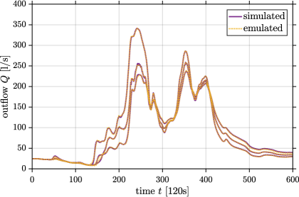
Figure 5: Final metamodel predictions. Three simulations (solid lines) and their approximations (dashed lines) are exemplarily shown. Solid and dashed lines that lie on top of each other correspond to the same inputs. Hence, the metamodel is considered as sufficiently accurate.

In Fig. 5 the simulated and emulated outflows are shown for three different input values in the experimental design that were randomly chosen. It is again ascertained that the obtained metamodel is sufficiently accurate for uncertainty quantification purposes. Although our regression approach does not explicitly guarantee the absence of negative outflow predictions, that would be unphysical, such predictions are not observed in our experiments.

3 Sensitivity analysis

Now we want to perform a global sensitivity analysis of the urban drainage simulator. Variance-based sensitivity analysis is based on apportioning the variance of a model response quantity among several uncertain input variables [26, 27]. This provides relevant insights into the model in question and gives rise to model reduction schemes [17, 18], e.g. one could construct a simplified model by fixing relatively unimportant parameters to their nominal values and varying only the most influential parameters. For a single response quantity, sensitivity measures such as Sobol’ indices can be efficiently computed with the aid of surrogate models [85], e.g. for a PCE one can estimate the sensitivities by a postprocessing of the expansion coefficients [86]. In the vector-valued case, one would have to estimate the sensitivity indices for each output quantity separately. If the model predictions are high-dimensional, such as the time series in almost every hydrological study, this would become inconvenient and time-consuming.

An original solution to this problem is proposed in this section. It is based on the combined metamodeling approach presented in the last section. Instead of computing the desired Sobol’ indices for the time-variant outflows directly, we consider the indices of the principal components first. Then we investigate how the obtained results can be reused for assessing the sensitivities of the discharge. As it turns out, this is feasible through a multivariate extension of the PCE coefficient postprocessing. This method for the global sensitivity analysis of high-dimensional outputs is explained in the following.

3.1 Sobol’ indices

Recall that we assumed the input variables $\bm{X}\sim\pi(\bm{x})=\pi_{1}(x_{1})\ldots\pi_{M}(x_{M})$ to be independent. For now, we consider a scalar-valued model response $\tilde{Y}_{f}=f(\bm{X})$ with finite variance, e.g. the catchment outflow $\tilde{Y}_{t}=f(\bm{X})$ at a time instant $t\in\{0,\ldots,N\}$ or a principal component $\tilde{Z}_{p}=f(\bm{X})$ with $p\in\{0,\ldots,N^{\prime}\}$. Variance-based global sensitivity analysis then rests on a decomposition of the model response into functions with an increasing number of input parameters. This so-called functional analysis of variance (ANOVA) or Hoeffding–Sobol decomposition [87, 88], which is sometimes also referred to as a high-dimensional model representation (HDMR) [89, 90], can be written as

$$f(\bm{X}) =f_{0}+\sum\limits_{1\leq i\leq M}f_{i}(X_{i})+\sum\limits_{1\leq i<j\leq M}f_{ij}(X_{i},X_{j})+\ldots+f_{1,\ldots,M}(X_{1},\ldots,X_{M})$$ (11)

$$=f_{0}+\sum\limits_{1\leq p\leq M}\sum\limits_{1\leq i_{1}<\ldots<i_{p}\leq M}f_{i_{1},\ldots,i_{p}}(X_{i_{1}},\ldots,X_{i_{p}})=\sum\limits_{u\subseteq\{1,\ldots,M\}}f_{u}(\bm{X}_{u}).$$

Here, $f_{0}$ is a constant and $f_{i}(X_{i})$ with $1\leq i\leq M$ are functions of a single variable. The last-mentioned functions are called main effects. Functions of more than one variable, such as $f_{ij}(X_{i},X_{j})$ with $1\leq i<j\leq M$, are called interactions. An intuitive indexing scheme for organizing the terms is introduced in the second line of Eq. 11. Here, $f_{u}(\bm{X}_{u})$ denotes the interaction of all variables $X_{i_{q}}$ with $i_{q}\in u$ that are contained in a certain set $u\subseteq\{1,\ldots,M\}$ and $f_{\varnothing}=f_{0}$ signifies the constant term.

The Hoeffding–Sobol decomposition is unique if one imposes the vanishing condition that $\mathds{E}[f_{u}(\bm{X}_{u})]=\int f_{u}(\bm{x}_{u})\,\pi_{i_{q}}(x_{i_{q}})\,\mathrm{d}x_{i_{q}}=0$ for $\varnothing\neq u\subseteq\{1,\ldots,M\}$ and $i_{q}\in u$. It follows that all terms but the constant have zero mean and they are mutually uncorrelated, i.e. for $u,v\subseteq\{1,\ldots,M\}$ with $u\neq v$ one has $\mathds{E}[f_{u}(\bm{X}_{u})f_{v}(\bm{X}_{v})]=\int f_{u}(\bm{x}_{u})f_{v}(\bm{x}_{v})\,\pi(\bm{x})\,\mathrm{d}\bm{x}=0$. Moreover, one can easily express the unconditional and conditional expectation values of the model response as

$$\mathds{E}[\tilde{Y}_{f}]=f_{0},\quad\mathds{E}[\tilde{Y}_{f}\>\!|\>\!X_{i}]=f_{0}+f_{i}(X_{i}),\quad\mathds{E}[\tilde{Y}_{f}\>\!|\>\!X_{i},X_{j}]=f_{0}+f_{i}(X_{i})+f_{j}(X_{j})+f_{ij}(X_{i},X_{j}).$$ (12)

Further conditional expectations are given analogously to Eq. 12. On this basis, one can obtain the terms $f_{0}=\mathds{E}[\tilde{Y}_{f}]$, $f_{i}(X_{i})=\mathds{E}[\tilde{Y}_{f}\>\!|\>\!X_{i}]-f_{0}$, $f_{ij}(X_{i},X_{j})=\mathds{E}[\tilde{Y}_{f}\>\!|\>\!X_{i},X_{j}]-f_{0}-f_{i}(X_{i})-f_{j}(X_{j})$ and so on recursively. One often utilizes that a real system model can be well described by an approximation where at most bivariate interactions are included, i.e. $f(\bm{X})\approx f_{0}+\sum_{1\leq i\leq M}f_{i}(X_{i})+\sum_{1\leq i<j\leq M}f_{ij}(X_{i},X_{j})$.

Note that the ANOVA/HDMR representation contains only finitely many summands, namely $\sum_{i=0}^{M}\binom{M}{i}=2^{M}$, all of which feature a finite variance. This allows one to meaningfully partition the variance of the model response $\mathrm{Var}[\tilde{Y}_{f}]=\mathds{E}[\tilde{Y}_{f}^{2}]-f_{0}^{2}$. The variance $\mathrm{Var}[\tilde{Y}_{f}]=\mathrm{Var}[\sum_{\varnothing\neq u\subseteq\{1,\ldots,M\}}f_{u}(\bm{X}_{u})]$ of the sum of the uncorrelated random variables in Eq. 11 is the sum of the individual variances

$$\mathrm{Var}[\tilde{Y}_{f}]=\sum\limits_{1\leq p\leq M}\sum\limits_{1\leq i_{1}<\ldots<i_{p}\leq M}\mathrm{Var}[f_{i_{1},\ldots,i_{p}}(X_{i_{1}},\ldots,X_{i_{p}})]=\sum\limits_{\varnothing\neq u\subseteq\{1,\ldots,M\}}\mathrm{Var}[f_{u}(\bm{X}_{u})].$$ (13)

Here, $\mathrm{Var}[f_{i_{1},\ldots,i_{p}}(X_{i_{1}},\ldots,X_{i_{p}})]=\mathds{E}[f_{i_{1},\ldots,i_{p}}^{2}(X_{i_{1}},\ldots,X_{i_{p}})]$ with $1\leq p\leq M$ is termed a partial variance. It quantifies the contribution of the combination of variables $(X_{i_{1}},\ldots,X_{i_{p}})$ to the total variance $\mathrm{Var}[\tilde{Y}_{f}]$. One then defines the Sobol’ index as the corresponding fraction of the total variance

$$S_{i_{1},\ldots,i_{p}}=\frac{\mathrm{Var}[f_{i_{1},\ldots,i_{p}}(X_{i_{1}},\ldots,X_{i_{p}})]}{\mathrm{Var}[\tilde{Y}_{f}]}.$$ (14)

The first-order indices $S_{i}=\mathrm{Var}[f_{i}(X_{i})]/\mathrm{Var}[\tilde{Y}_{f}]$ with $1\leq i\leq M$ measure the influence of the main effects. Similarly, the second-order indices $S_{ij}=\mathrm{Var}[f_{ij}(X_{i},X_{j})]/\mathrm{Var}[\tilde{Y}_{f}]$ with $1\leq i<j\leq M$ quantify the effect of the bivariate interactions. In total, there are $2^{M}-1$ sensitivity indices specified this way. They are often summarized by reference to the total Sobol’ index of a variable $X_{i_{q}}$ with $1\leq i_{q}\leq M$ [91]. It is defined as

$$T_{i_{q}}=\sum\limits_{1\leq p\leq M}\sum\limits_{1\leq i_{1}<\ldots<i_{q}<\ldots<i_{p}\leq M}S_{i_{1},\ldots,i_{q},\ldots,i_{p}}=\sum\limits_{\begin{subarray}{c}\varnothing\neq u\subseteq\{1,\ldots,M\}\\ i_{q}\in u\end{subarray}}S_{u}.$$ (15)

One can interpret the total index as the total effect due to the input parameter $X_{i_{q}}$, either in isolation or in conjunction with other variables. While the indices in Eq. 14 satisfy $\sum_{1\leq p\leq M}\sum_{1\leq i_{1}<\ldots<i_{p}\leq M}S_{i_{1},\ldots,i_{p}}=1$, the total Sobol’ indices in Eq. 15 do not have to add up to one. Instead one has $0\leq T_{i_{q}}\leq 1$ and $\sum_{1\leq i_{q}\leq M}T_{i_{q}}\geq 1$ for the total indices.

Note that the conditional expectations $\mathds{E}[\tilde{Y}_{f}\>\!|\>\!X_{i}]$ and $\mathds{E}[\tilde{Y}_{f}\>\!|\>\!X_{i},X_{j}]$ in Eq. 12 are actually random variables. This follows from their dependence on $X_{i}$ and $X_{j}$. Hence, one can consider the variances of the conditional expectation values. These are given as

$$\mathrm{Var}[\mathds{E}[\tilde{Y}_{f}\>\!|\>\!X_{i}]]=\mathrm{Var}[f_{i}(X_{i})],\quad\mathrm{Var}[\mathds{E}[\tilde{Y}_{f}\>\!|\>\!X_{i},X_{j}]]=\mathrm{Var}[f_{i}(X_{i})]+\mathrm{Var}[f_{j}(X_{j})]+\mathrm{Var}[f_{ij}(X_{i},X_{j})].$$ (16)

While the conditional expectations are related to the terms of the ANOVA/HDMR decomposition, their variances in Eq. 16 admit interesting interpretations of the partial variances and Sobol’ indices. For instance, the first partial variances are given as $\mathrm{Var}[f_{i}(X_{i})]=\mathrm{Var}[\mathds{E}[\tilde{Y}_{f}\>\!|\>\!X_{i}]]$ and $\mathrm{Var}[f_{ij}(X_{i},X_{j})]=\mathrm{Var}[\mathds{E}[\tilde{Y_{f}}\>\!|\>\!X_{i},X_{j}]]-\mathrm{Var}[f_{i}(X_{i})]-\mathrm{Var}[f_{j}(X_{j})]$, respectively. Consequentially, the Sobol’ indices can be expressed as $S_{i}=\mathrm{Var}[\mathds{E}[\tilde{Y}_{f}\>\!|\>\!X_{i}]]/\mathrm{Var}[\tilde{Y}_{f}]$ and $S_{ij}=\mathrm{Var}[\mathds{E}[\tilde{Y}_{f}\>\!|\>\!X_{i},X_{j}]]/\mathrm{Var}[\tilde{Y}_{f}]-S_{i}-S_{j}$. As a consequence of Eq. 13 and the law of total variance, the total index can be written as $T_{i}=1-\mathrm{Var}[\mathds{E}[\tilde{Y}_{f}\>\!|\>\!\bm{X}_{\sim i}]]/\mathrm{Var}[\tilde{Y}_{f}]=\mathds{E}[\mathrm{Var}[\tilde{Y}_{f}\>\!|\>\!\bm{X}_{\sim i}]]/\mathrm{Var}[\tilde{Y}_{f}]$, where we have defined $\bm{X}_{\sim i}=(X_{1},\ldots,X_{i-1},X_{i+1},\ldots,X_{M})$.

Notice that for dependent input variables $\bm{X}\sim\pi(\bm{x})\neq\pi_{1}(x_{1})\ldots\pi_{M}(x_{M})$, the model representation in Eq. 11 contains terms of increasing input dimensionality and, hence, the variance decomposition in Eq. 13, is not unique anymore [92, 93]. Although one could still use $S_{i}=\mathrm{Var}[\mathds{E}[\tilde{Y}_{f}\>\!|\>\!X_{i}]]/\mathrm{Var}[\tilde{Y}_{f}]$ as the definition of a sensitivity measure, it would reflect both the model structure and the input dependencies [94]. The interpretation is therefore not as straightforward as in the case of independent inputs.

3.2 Multivariate output

So far we have discussed the sensitivity analysis of a scalar-valued response variable $\tilde{Y}_{f}=f(\bm{X})$ only, but model responses such as $\tilde{\bm{Y}}=\mathcal{M}_{\bm{d}}(\bm{X})$ in Eq. 2 are often vector-valued. Two related ways of defining sensitivity measures for multivariate outputs have been established in the literature. First, in [95, 96] a multivariate generalization of the Sobol’ indices was proposed that is based on the trace of a decomposition of the model output covariance matrix. Second, in [97] it was suggested to expand the model outputs in a certain basis first, and then to determine the standard Sobol’ indices of the expansions coefficients with respect to the uncertain model inputs. A comparison of those approaches is found in [98].

Determining the Sobol’ indices of the principal components is a special case of the last-mentioned output decomposition approach [99, 100]. It lends itself to the multivariate sensitivity analysis of models with time-dependent [101, 102] or spatially distributed [103, 104] responses quantities. However, the sensitivity measures of the principal components obtained this way, or of artificial coefficients in general, are difficult to interpret. We therefore establish a link between the sensitivities of the expansion coefficients and the ones of the physically meaningful model outputs. This possibility has been often overlooked.

In our case, the principal components $\tilde{\bm{Z}}$ and the actual model outputs $\tilde{\bm{Y}}$ are related through the orthogonal transformation $\tilde{\bm{Z}}=\bm{\Phi}^{\top}(\tilde{\bm{Y}}-\bm{\mu}_{\tilde{\bm{Y}}})$ in Eq. 32, and vice versa through $\tilde{\bm{Y}}=\bm{\mu}_{\tilde{\bm{Y}}}+\bm{\Phi}\tilde{\bm{Z}}$ in Eq. 33. For $t=0,\ldots,N$ the model outputs are given as $\tilde{Y}_{t}=\mu_{\tilde{Y}_{t}}+\sum_{p=0}^{N}\tilde{Z}_{p}\phi_{p,t}$. Here, $\mu_{\tilde{Y}_{t}}$ is the $t$-th entry of the mean vector $\bm{\mu}_{\tilde{\bm{Y}}}$ and $\phi_{p,t}$ is the corresponding entry of the $p$-th eigenvector $\bm{\phi}_{p}$ of the covariance matrix in Eq. 30. One consequentially has $\mathds{E}[\tilde{Y}_{t}\>\!|\>\!X_{i}]=\mu_{\tilde{Y}_{t}}+\sum_{p=0}^{N}\mathds{E}[\tilde{Z}_{p}\>\!|\>\!X_{i}]\phi_{p,t}$ for the conditional expectation of $\tilde{Y}_{t}$ with respect to an input $X_{i}$ with $i\in\{1,\ldots,M\}$. The variance of this conditional expectation is given as

$$\mathrm{Var}[\mathds{E}[\tilde{Y}_{t}\>\!|\>\!X_{i}]]=\sum\limits_{p=0}^{N}\mathrm{Var}[\mathds{E}[\tilde{Z}_{p}\>\!|\>\!X_{i}]]\phi^{2}_{p,t}+2\sum\limits_{p<q}\mathrm{Cov}[\mathds{E}[\tilde{Z}_{p}\>\!|\>\!X_{i}],\mathds{E}[\tilde{Z}_{q}\>\!|\>\!X_{i}]]\phi_{p,t}\phi_{q,t}.$$ (17)

One can now relate the first-order Sobol’ index of the output $\tilde{Y}_{t}$ with respect to the input $X_{i}$ to the corresponding indices of the principal components $\tilde{Z}_{p}$ for $p=0,\ldots,N$. From Eq. 17 one obtains

$$S_{i}^{\tilde{Y}_{t}}=\frac{\mathrm{Var}[\mathds{E}[\tilde{Y}_{t}\>\!|\>\!X_{i}]]}{\mathrm{Var}[\tilde{Y}_{t}]}=\sum\limits_{p=0}^{N}S_{i}^{\tilde{Z}_{p}}\frac{\mathrm{Var}[\tilde{Z}_{p}]}{\mathrm{Var}[\tilde{Y}_{t}]}\phi^{2}_{p,t}+2\sum\limits_{p<q}\frac{\mathrm{Cov}[\mathds{E}[\tilde{Z}_{p}\>\!|\>\!X_{i}],\mathds{E}[\tilde{Z}_{q}\>\!|\>\!X_{i}]]}{\mathrm{Var}[\tilde{Y}_{t}]}\phi_{p,t}\phi_{q,t}.$$ (18)

Here, $S_{i}^{\tilde{Z}_{p}}=\mathrm{Var}[\mathds{E}[\tilde{Z}_{p}\>\!|\>\!X_{i}]]/\mathrm{Var}[\tilde{Z}_{p}]$ denotes the Sobol’ index of a principal component $\tilde{Z}_{p}$ with respect to an input variable $X_{i}$. Hence, Eq. 18 allows one to reuse these indices for the sensitivity analysis of original outputs. It is noted that the covariances $\mathrm{Cov}[\mathds{E}[\tilde{Z}_{p}\>\!|\>\!X_{i}],\mathds{E}[\tilde{Z}_{q}\>\!|\>\!X_{i}]]$ of the conditional expectations $\mathds{E}[\tilde{Z}_{p}\>\!|\>\!X_{i}]$ and $\mathds{E}[\tilde{Z}_{q}\>\!|\>\!X_{i}]$ for $p,q=1,\ldots,N$ with $p\neq q$ emerge in the above expression. One can proceed similarly for the second-order and higher indices. In practice, when instead of Eq. 33 a reduced number of principal components with $N^{\prime}\leq N$ is used in Eq. 35, one employs the induced approximations of Eqs. 17 and 18.

3.3 Practical computation

The practical computation of the discussed sensitivity measures in Eqs. 14 and 15 can be based on Monte Carlo simulation [105, 106]. As it was originally proven in [86], however, one can obtain the Sobol’ indices of an output quantity from an appropriate rearrangement of a PCE of that quantity, too. This is usually more efficient and, in our case, it is also more convenient. Since we employ a polynomial representation of the principal components, their Sobol’ indices can be estimated right away. Besides, as it is demonstrated next, one can extract the corresponding indices of the discharge. This allows for a time-variant global sensitivity analysis.

The terms of $\tilde{z}_{p}(\bm{X})=\sum_{\bm{\alpha}\in\mathds{N}^{M}}a_{p,\bm{\alpha}}\Psi_{\bm{\alpha}}(\bm{X})$ in Eq. 8 can be reordered for all $p=0,\dots,N^{\prime}$ so as to match the structure of the Hoeffding decomposition in Eq. 11, i.e. the PCE terms are grouped according to their input variables. To that effect, let us define the set of multi-indices $\mathcal{A}_{u}=\{(\alpha_{1},\ldots,\alpha_{M})\in\mathds{N}^{M}\colon k\in u\Leftrightarrow\alpha_{k}\neq 0\}$ for any non-empty set $u\subseteq\{1,\ldots,M\}$. Following this, the rearrangement into terms with an increasing number of input variables is given as

$$\tilde{z}_{p}(\bm{X})=a_{p,\bm{0}}+\sum\limits_{\varnothing\neq u\subseteq\{1,\ldots,M\}}\sum\limits_{\bm{\alpha}\in\mathcal{A}_{u}}a_{p,\bm{\alpha}}\Psi_{\bm{\alpha}}(\bm{X})=a_{p,\bm{0}}+\sum\limits_{\varnothing\neq u\subseteq\{1,\ldots,M\}}\tilde{z}_{p,u}(\bm{X}_{u}).$$ (19)

Each summand $\tilde{z}_{p,u}(\bm{X})=\sum_{\bm{\alpha}\in\mathcal{A}_{u}}a_{p,\bm{\alpha}}\Psi_{\bm{\alpha}}(\bm{X})$ in Eq. 19 contains only the PCE terms with multi-indices $\bm{\alpha}\in\mathcal{A}_{u}$. Since we have $\mathrm{Var}[\tilde{z}_{p}(\bm{X})]=\sum_{\bm{\alpha}\in\mathds{N}^{M}\setminus\{\bm{0}\}}a_{p,\bm{\alpha}}^{2}$ and $\mathrm{Var}[\tilde{z}_{p,u}(\bm{X}_{u})]=\sum_{\bm{\alpha}\in\mathcal{A}_{u}}a_{p,\bm{\alpha}}^{2}$, the Sobol’ indices in Eq. 14 can be easily determined from the PCE coefficients. For instance, the first-order Sobol’ index of the principal component $\tilde{Z}_{p}$ with respect to the input parameter $X_{i}$ is obtained for $u=\{i\}$ as

$$S_{i}^{\tilde{Z}_{p}}=\frac{\sum_{\bm{\alpha}\in\mathcal{A}_{\{i\}}}a_{p,\bm{\alpha}}^{2}}{\sum_{\bm{\alpha}\in\mathds{N}^{M}\setminus\{\bm{0}\}}a_{p,\bm{\alpha}}^{2}}.$$ (20)

The first-order index $S_{i}^{\tilde{Y}_{t}}$ of the time-variant output $\tilde{Y}_{t}$ with respect to an input $X_{i}$ is given by Eq. 18. This formula contains the covariances $\mathrm{Cov}[\mathds{E}[\tilde{Z}_{p}\>\!|\>\!X_{i}],\mathds{E}[\tilde{Z}_{q}\>\!|\>\!X_{i}]]$ of the conditional expectations $\mathds{E}[\tilde{Z}_{p}\>\!|\>\!X_{i}]$ and $\mathds{E}[\tilde{Z}_{q}\>\!|\>\!X_{i}]$ with $1\leq p<q\leq N$. According to Eq. 12 one has $\mathds{E}[\tilde{Z}_{p}\>\!|\>\!X_{i}]=a_{p,\bm{0}}+\sum_{\bm{\alpha}\in\mathcal{A}_{\{i\}}}a_{p,\bm{\alpha}}\Psi_{\bm{\alpha}}(\bm{X})$ and an analogous expression for $\mathds{E}[\tilde{Z}_{q}\>\!|\>\!X_{i}]$. Due to the orthogonality of the polynomial basis, the covariance terms can then be written as

$$\mathrm{Cov}[\mathds{E}[\tilde{Z}_{p}\>\!|\>\!X_{i}],\mathds{E}[\tilde{Z}_{q}\>\!|\>\!X_{i}]]=\sum\limits_{\bm{\alpha}\in\mathcal{A}_{\{i\}}}a_{p,\bm{\alpha}}a_{q,\bm{\alpha}}.$$ (21)

The first-order index $S_{i}^{\tilde{Y}_{t}}$ is eventually determined by Eq. 18 with Eqs. 20 and 21. In practice, instead of the infinite series in Eq. 8, one uses the truncated one in Eq. 9 in order to obtain approximations of the Sobol’ indices.

Following this discussion, we compute the Sobol’ indices $S_{i}^{\tilde{Z}_{p}}$ and $S_{i}^{\tilde{Y}_{t}}$ for all principal components $\tilde{Z}_{p}$ with $p=0,\ldots,8$ and time-dependent discharges $\tilde{Y}_{t}$ with $t=0,\ldots,600$, with respect to all inputs $X_{i}$ with $i=1,\ldots,8$. The results are plotted in Fig. 6.

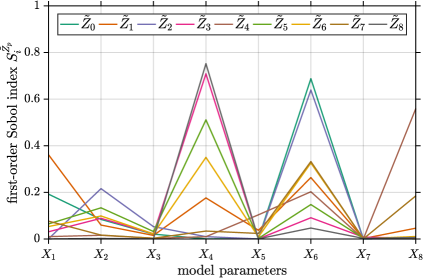
(a) Principal components.

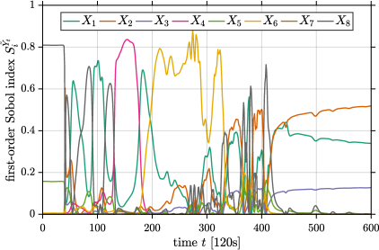
(b) Time-variant outflow.

Figure 6: First-order Sobol’ indices. The first Sobol’ indices of the principal components are shown in Fig. 6. They are obtained by an analysis of the corresponding PCE coefficients. The first Sobol’ indices of the time-variant outflow are plotted in Fig. 6 They can be reconstructed from the sensitivity indices of the principal components. While the parameters $X_{4}$ and $X_{6}$ are revealed to be the most influential, $X_{7}$ contributes insignificantly.

First of all, Fig. 6 shows the first-order Sobol’ indices of the principal components $\tilde{Z}_{p}$ with respect to the input variables $X_{i}$. On the basis of Eq. 20, the indices are straightforwardly extracted from the corresponding PCEs. Second of all, the first-order Sobol’ indices of the time-variant outputs $\tilde{Y}_{t}$ with respect to the inputs are depicted in Fig. 6. They are computed with the aid of Eqs. 18, 20 and 21 in a further postprocessing step.

Regarding the contribution to the variances of the principal components, Fig. 6 reveals that the input parameters $X_{4}$ and $X_{6}$ are the most important. They describe the depression storage height of the impervious and pervious areas, respectively. While $X_{6}$ influences the first principal components, $X_{4}$ mainly impacts on the last. The model input parameter $X_{7}$, describing the percentage of the impervious area without depression storage, hardly contributes at all to the variances of the principal components. While the sensitivities of the principal components with respect to the input parameters are difficult to interpret, the time-evolution of the Sobol’ indices in Fig. 6 may be more intuitive to grasp. In roughly the interval $t/120\,\mathrm{s}\in[100,400]$, which corresponds to heavy rain and high outflow in Fig. 2, the parameters $X_{4}$ and $X_{6}$ are the most dominant. In contrast, $X_{7}$ is again the least influential parameter on the whole.

4 Bayesian calibration

We now turn towards probabilistic model calibration. The goal is to infer the unknown hydrological parameters with the available outflow data. Bayesian inference establishes a principled framework for data analysis and uncertainty reduction [28, 29]. Unknown parameters can be inferred from indirectly related measurements. A prior probability distribution is assigned to the unknown parameters, which reflects the epistemic uncertainty of the parameters before the data are analyzed. The prior is then conditioned on the realized data, which gives rise to the posterior distribution. It represents the reduced uncertainty after the data have been processed. Markov chain Monte Carlo is usually used in order to numerically explore the posterior [34, 35]. Beyond parametric uncertainties, Bayesian inference allows one to cope with model discrepancy as well [30, 31]. This is especially important in hydrological applications where predictions are typically uncertain and biased [107, 108].

In this section, two different Bayesian models are employed in order to account for the high level of uncertainty and error in hydrological model predictions. The first model is a formulation of nonlinear inverse modeling with an unknown level of additive noise. A residual term following a multivariate Gaussian distribution with zero mean and unknown variance is used to represent the deviation of the predicted outflows from the measured values. The deviations at different times are assumed to be uncorrelated. Measurement uncertainty and modeling errors are lumped together in this formulation. The unknown parameters as well as the unknown error variance can be inferred with the first simple model.

A more complex Bayesian model is devised that allows us to additionally capture error correlation and model discrepancy. The deviations between the model predictions and the data are now represented as the sum of two terms. Similar as in the simple model, the first term represents Gaussian random errors, but now the errors at different times are allowed to be correlated. On top of that, the second term represents a systematic model discrepancy as a low-order polynomial function of time. This more realistic model does not only allow us to estimate the uncertain parameters and the noise level and its correlation structure, it also enables us to learn the discrepancy function. It is remarked that the discrepancy here pertains to both the model and the analyzed rainfall event, i.e. it captures the systematic error of the model over the duration of the event.

4.1 Independent random errors

Recall that the measurement data $\bm{y}=(y_{0},\ldots,y_{600})^{\top}$ comprise the observations of the outflow $y_{i}=Q(t_{i})$ for $i=0,\ldots,600$. Assuming that random measurement errors act additively and independently on the forward model predictions, in the first simple model the measured data are represented as

$$\bm{y}=\mathcal{M}_{\bm{d}}(\bm{x})+\bm{\varepsilon}.$$ (22)

Here, $\bm{\varepsilon}$ is a realization of a random vector with a Gaussian distribution $\pi(\bm{\varepsilon}\>\!|\>\!\sigma)=\mathcal{N}(\bm{\varepsilon}\>\!|\>\!\bm{0},\sigma^{2}\bm{I})$, where the noise level $\sigma>0$ is unknown. Consequently the following statistical model arises

$$\pi_{1}(\bm{y}\>\!|\>\!\bm{x},\sigma)=\mathcal{N}(\bm{y}\>\!|\>\!\mathcal{M}_{\bm{d}}(\bm{x}),\sigma^{2}\bm{I}).$$ (23)

The likelihood function is simply $\mathcal{L}_{1}(\bm{x},\sigma)=\mathcal{N}(\bm{y}\>\!|\>\!\mathcal{M}_{\bm{d}}(\bm{x}),\sigma^{2}\bm{I})$. Instead of merely maximizing the likelihood, a fully Bayesian approach is pursued. For any given prior distribution $\pi_{1}(\bm{x},\sigma)$, the corresponding posterior is

$$\pi_{1}(\bm{x},\sigma\>\!|\>\!\bm{y})\propto\mathcal{L}_{1}(\bm{x},\sigma)\pi_{1}(\bm{x},\sigma).$$ (24)

In order to complete the setup, we specify a joint prior of the unknowns with the product structure $\pi_{1}(\bm{x},\sigma)=\pi_{1}(\bm{x})\pi_{1}(\sigma)$ and $\pi_{1}(\bm{x})=\pi_{1}(x_{1})\ldots\pi_{1}(x_{8})$. While the previously used uniform marginals were motivated by coverage considerations, we now respect the following expert recommendations. The priors for the hydrological parameters $x_{i}\in[\underline{x}_{i},\overline{x}_{i}]$ are normal distributions $\pi_{1}(x_{i})=\mathcal{N}(x_{i}\>\!|\>\!\mu_{x_{i}},\sigma_{x_{i}}^{2},\underline{x}_{i},\overline{x}_{i})$ truncated at the respective parameter bounds $\underline{x}_{i}$ and $\overline{x}_{i}$. Before the truncation, the distributions are centered around the midpoint $\mu_{x_{i}}=(\underline{x}_{i}+\overline{x}_{i})/2$ and their standard deviations $\sigma_{i}=(\overline{x}_{i}-\underline{x}_{i})/6$ are set to the sixth part of the admissible range. Note that the prior for the hydrological parameters is different from the uniform distribution that the experimental design was sampled from. A uniform distribution $\pi_{1}(\sigma)=\mathcal{U}(\sigma\>\!|\>\!\underline{\sigma},\overline{\sigma})$ with $\underline{\sigma}=0\times\mathrm{l/s}$ and $\overline{\sigma}=100\times\mathrm{l/s}$ is selected as the prior for the unknown noise level $\sigma$. The lower bound emerges naturally, whereas the upper bound is chosen so that it is highly probable that the true or best value is really contained in the supported interval.

4.2 Systematic model discrepancy

The second model is more sophisticated in that it also acknowledges other sources of uncertainty and error. In particular, model discrepancy and random error correlation are captured. We start the discussion by representing the measurement data as

$$\bm{y}=\mathcal{M}_{\bm{d}}(\bm{x})+\bm{\delta}(\bm{b})+\bm{\varepsilon}.$$ (25)

This is the sum of the model response $\mathcal{M}_{\bm{d}}(\bm{x})$ at the true $\bm{x}$ and two other terms that allow for a refined treatment of discrepancy and noise. The systematic modeling errors are absorbed into the term $\bm{\delta}(\bm{b})$, whereas $\bm{\varepsilon}$ captures the noise. We assume that the discrepancy is an unknown function of time that can be sufficiently well represented as

$$\delta(\bm{b},t)=\sum\limits_{\alpha=0}^{\gamma}b_{\alpha}\Psi_{\alpha}(t).$$ (26)

Here, $\{\Psi_{\alpha}(t)\}_{\alpha=0}^{\gamma}$ is a function basis with $\Gamma=\gamma+1$ elements and $\bm{b}=(b_{0},\ldots,b_{\gamma})^{\top}$ denotes the unknown coefficients. The values $\delta_{i}(\bm{b})=\delta(\bm{b},t_{i})$ of the discrepancy function at the measurement instants $t_{i}$ for $i=0,\ldots,600$ generate the discrepancy vector $\bm{\delta}(\bm{b})=(\delta_{0}(\bm{b}),\ldots,\delta_{600}(\bm{b}))^{\top}$.

The term $\bm{\varepsilon}$ is a realization of a random vector following a multivariate Gaussian distribution $\pi(\bm{\varepsilon}\>\!|\>\!\sigma,\tau)=\mathcal{N}(\bm{\varepsilon}\>\!|\>\!\bm{0},\bm{\Sigma}(\sigma,\tau))$ with an unknown covariance matrix $\bm{\Sigma}(\sigma,\tau)$. For $i,j=0,\ldots,600$ the entries of the covariance matrix are represented as

$$\Sigma_{i,j}(\sigma,\tau)=\sigma^{2}\exp\left(-\frac{\lvert t_{i}-t_{j}\rvert}{\tau}\right).$$ (27)

As before, the standard deviation $\sigma$ determines the noise level. The additionally introduced correlation length $\tau$ establishes a characteristic time scale of the error correlation. Both parameters $\sigma$ and $\tau$ describing the covariance structure of the error process are unknown. In total, we have established the probabilistic data model

$$\pi_{2}(\bm{y}\>\!|\>\!\bm{x},\bm{b},\sigma,\tau)=\mathcal{N}(\bm{y}\>\!|\>\!\mathcal{M}_{\bm{d}}(\bm{x})+\bm{\delta}(\bm{b}),\bm{\Sigma}(\sigma,\tau)).$$ (28)

The likelihood function $\mathcal{L}_{2}(\bm{x},\bm{b},\sigma,\tau)=\mathcal{N}(\bm{y}\>\!|\>\!\mathcal{M}_{\bm{d}}(\bm{x})+\bm{\delta}(\bm{b}),\bm{\Sigma}(\sigma,\tau))$ arises as a result. If one has a joint prior $\pi_{2}(\bm{x},\bm{b},\sigma,\tau)$, one obtains the posterior distribution by

$$\pi_{2}(\bm{x},\bm{b},\sigma,\tau\>\!|\>\!\bm{y})\propto\mathcal{L}_{2}(\bm{x},\bm{b},\sigma,\tau)\pi_{2}(\bm{x},\bm{b},\sigma,\tau).$$ (29)

Some prior specifications are now overdue. We impose a joint prior distribution with the block-wise independence structure $\pi_{2}(\bm{x},\bm{b},\sigma,\tau)=\pi_{2}(\bm{x})\pi_{2}(\bm{b})\pi_{2}(\sigma)\pi_{2}(\tau)$. While the priors $\pi_{2}(\bm{x})=\pi_{1}(\bm{x})$ and $\pi_{2}(\sigma)=\pi_{1}(\sigma)$ are not altered, we only have to set $\pi_{2}(\bm{b})$ and $\pi_{2}(\tau)$. The latter is chosen as $\pi_{2}(\tau)=\mathcal{U}(\tau\>\!|\>\!\underline{\tau},\overline{\tau})$ with the lower bound $\underline{\tau}=0\times 120\,\mathrm{s}$ and a conservatively high upper bound $\overline{\tau}=100\times 120\,\mathrm{s}$.

We believe that the discrepancy $\delta(\bm{b},t)$ is a rather smooth function of time. It is thus expanded in terms of the first normalized Legendre polynomials $\{\Psi_{\alpha}(t)\}_{\alpha=0}^{\gamma}$ up to rather low degree $\gamma=5$. These are the polynomials shown in Fig. 4. The time variable is translated and stretched such that it follows the standard uniform distribution in Table 2. In fact there is no need to be picky while choosing the polynomial family here. Since the expansion coefficients $\bm{b}$ are mere tuning parameters which do not correspond to physically interpretable quantities, the specification of the prior $\pi_{2}(\bm{b})=\pi_{2}(b_{0})\ldots\pi_{2}(b_{5})$ is a bit delicate. We opt for Laplace distributions $\pi_{2}(b_{i})=\mathrm{Laplace}(b_{i}\>\!|\>\!\mu_{x_{i}},s_{x_{i}})=(2s_{x_{i}})^{-1}\exp(-\lvert b_{i}-\mu_{x_{i}}\rvert/s_{x_{i}})$ for all $i=0,\ldots,5$. They peak at the mean $\mu_{x_{i}}=0$ and have the scale parameter $s_{x_{i}}=10$ which leads to a standard deviation $\sigma_{x_{i}}=s_{x_{i}}\sqrt{2}\approx 15$.

The double-exponential density $\mathrm{Laplace}(b_{i}\>\!|\>\!\mu_{x_{i}},s_{x_{i}})$ decays exponentially with the absolute difference from the mean, whereas the bell-shaped density $\mathcal{N}(b_{i}\>\!|\>\!\mu_{x_{i}},\sigma_{x_{i}}^{2})=(2\pi\sigma_{x_{i}}^{2})^{-1/2}\exp(-(b_{i}-\mu_{x_{i}})^{2}/(2\sigma_{x_{i}}^{2}))$ dies down with the squared difference. Accordingly, the Laplace distribution has a spikier peak and fatter tails than the Gaussian at the same time. Both sparsity of the coefficient vector and robustness with respect to the prior choice are promoted that way. While sparsity is not our main concern at this point, robustness can be indeed adduced as an argument for the Laplace prior. The specification of the scale parameter, however, remains more or less arbitrary after all.

4.3 Posterior distributions

Now we perform fully Bayesian analyses by computing the two posterior distributions $\pi_{1}(\bm{x},\sigma\>\!|\>\!\bm{y})$ and $\pi_{2}(\bm{x},\bm{b},\sigma,\tau\>\!|\>\!\bm{y})$ by means of MCMC sampling. The obtained surrogate model $\hat{\mathcal{M}}_{p}(\bm{x})$ is used in place of the original simulator $\mathcal{M}_{\bm{d}}(\bm{x})$ throughout the analyses. A random walk Metropolis algorithm with a Gaussian proposal distribution is deployed. Thirty parallel chains with $10^{6}$ MCMC iterations are run for both Bayesian models. For the first model the parameters $(\bm{x},\sigma)$ are updated altogether, while for the second model $\bm{x}$ and $(\sigma,\tau,\bm{b})$ are updated in two separate blocks. Roughly speaking, the posterior computations take half a day for the simple and about a week for the more complex model. The non-diagonal covariance matrix and the block-wise MCMC updates for the second model are responsible for the runtime difference.

Remember that a single run of the original SWMM simulator takes around twenty seconds to terminate. Notwithstanding that this is actually quite fast, in case the original model would be used in the MCMC algorithms described above, the total runtime would amount to more than two hundred days. On top of the final runs, MCMC always demands the execution of preliminary runs on the basis of which the algorithm is tuned and convergence is monitored. Since this would be obviously infeasible with the original SWMM simulator, only the employment of the fast surrogate model here enables us to carry out a Bayesian uncertainty analysis.

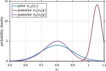
(a) Model parameter $x_{1}$.

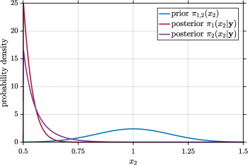
(b) Model parameter $x_{2}$.

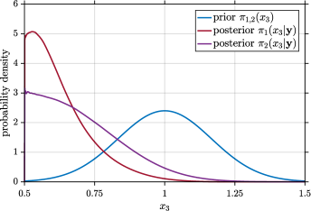
(c) Model parameter $x_{3}$.

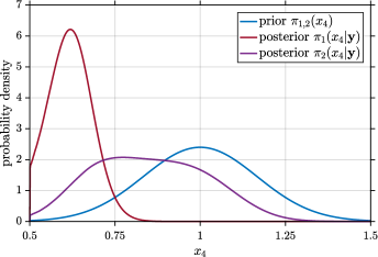
(d) Model parameter $x_{4}$.

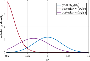
(e) Model parameter $x_{5}$.

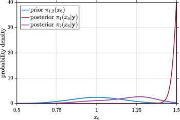
(f) Model parameter $x_{6}$.

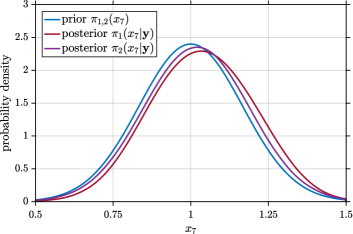
(g) Model parameter $x_{7}$.

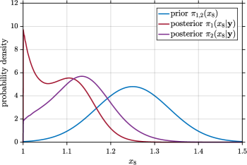
(h) Model parameter $x_{8}$.

Figure 7: Posterior marginals for the hydrological model. The posterior marginals of the parameters $x_{1},\ldots,x_{8}$ are shown above. While the marginal of $x_{8}$ shown in Fig. 7 features a distinct posterior structure, the posterior of $x_{7}$ in Fig. 7 is hardly different from its prior. The other marginals peak close to or directly at one of the parameter bounds.

First of all, we discuss the posterior marginals of the uncertain hydrological parameters $\bm{x}$. All marginals shown in the following are obtained through kernel density estimation. For $i=1,\ldots,8$ the marginals $\pi_{1}(x_{i}\>\!|\>\!\bm{y})$ and $\pi_{2}(x_{i}\>\!|\>\!\bm{y})$ of both Bayesian models are plotted in Fig. 7. Some marginals of the simple model feature posterior modes close to their bounds, i.e. see Figs. 7, 7 and 7 where the posteriors of $x_{1}$, $x_{3}$ and $x_{4}$ are depicted. Other marginals peak directly at the parameter bounds, i.e. the marginals of $x_{2}$, $x_{5}$ and $x_{6}$ in Figs. 7, 7 and 7, respectively. The posterior of $x_{7}$ in their bounds, i.e. see Fig. 7 is hardly different from the prior. A more complex structure is found in the marginal of $x_{8}$ that is shown in their bounds, i.e. see Fig. 7. It has two modes, one of which peaks at the lower parameter bound. As compared to the simple model, the marginal posteriors of the second model with the discrepancy term are generally flattened out and shifted towards the prior means.

The posterior marginals of the parameters describing the random error model are shown in Fig. 8. As it can be seen from Fig. 8, the marginal $\pi_{1}(\sigma\>\!|\>\!\bm{y})$ suggests a higher value of the standard deviation $\sigma$ than the marginal $\pi_{2}(\sigma\>\!|\>\!\bm{y})$. The reason is that according to the first model all errors are attributed to independent noise only. In the second model, those errors are also captured by the error correlation and model discrepancy. The marginal $\pi_{2}(\tau\>\!|\>\!\bm{y})$ of the correlation length $\tau$ is plotted in Fig. 8. It concentrates around a surprisingly low value. We speculate that the introduction and estimation of the discrepancy term effectively decorrelates the remaining sources of random error, which would explain this observation. In Fig. 8 all marginals $\pi_{2}(b_{i}\>\!|\>\!\bm{y})$ of the coefficients $b_{i}$ with $i=0,\ldots,5$ are shown. Their actual units are discarded for the sake of simplicity. It is interesting to note that the parameters $\bm{b}$ of the discrepancy function are estimated quite clearly. Especially the constant and the linear term with their coefficients $b_{0}$ and $b_{1}$ have pronounced posterior shapes.

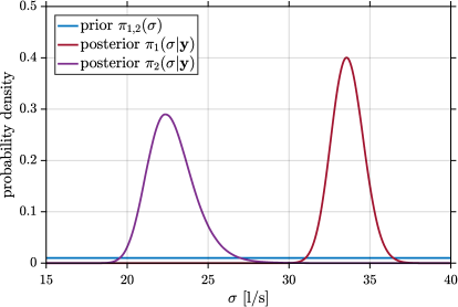
(a) Noise level $\sigma$.

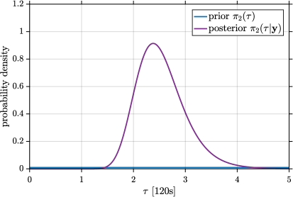
(b) Correlation length $\tau$.

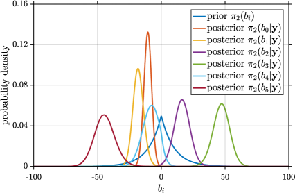
(c) Discrepancy coefficients $b_{i}$.

Figure 8: Posterior marginals for the error model. The posterior marginals of the error model parameters $\sigma,\tau$ and $b_{0},\ldots,b_{5}$ are depicted. It can be understood from Fig. 8 that the posterior estimate of the noise level parameter $\sigma$ is higher for the first error model than for the second one. The reason is that the latter involves further sources of uncertainty that are parametrized through $\tau$ and $b_{0},\ldots,b_{5}$.

Some summaries of the posterior distributions $\pi_{1}(\bm{x},\sigma\>\!|\>\!\bm{y})$ and $\pi_{2}(\bm{x},\bm{b},\sigma,\tau\>\!|\>\!\bm{y})$ are compiled in Table 4. These are point estimates of the unknown parameters, e.g. the posterior mean vectors $(\hat{\bm{x}},\hat{\sigma})=\mathds{E}[\bm{x},\sigma\>\!|\>\!\bm{y}]$ and $(\hat{\bm{x}},\hat{\bm{b}},\hat{\sigma},\hat{\tau})=\mathds{E}[\bm{x},\bm{b},\sigma,\tau\>\!|\>\!\bm{y}]$. Quantities whose dimension does not equal one are expressed in comparison to the units that were previously adopted. Posteriors that peak at the prior bounds are not summarized well by their mean values only. Therefore the modes $(\hat{\bm{x}},\hat{\sigma})_{\mathrm{MAP}}=\operatorname{arg\,max}_{\bm{x},\sigma}\pi_{1}(\bm{x},\sigma\>\!|\>\!\bm{y})$ and $(\hat{\bm{x}},\hat{\bm{b}},\hat{\sigma},\hat{\tau})_{\mathrm{MAP}}=\operatorname{arg\,max}_{\bm{x},\bm{b},\sigma,\tau}\pi_{2}(\bm{x},\bm{b},\sigma,\tau\>\!|\>\!\bm{y})$ of the joint posterior densities are shown, too. They have been obtained through maximizing the logarithms of the unnormalized posterior densities, i.e. the log–likelihood function plus the log–prior density. Note that the individual components of the joint posterior density mode do not have to coincide with the maxima of the marginal densities.

Table 4: Posterior summaries.

		$\hat{x}_{1}$	$\hat{x}_{2}$	$\hat{x}_{3}$	$\hat{x}_{4}$	$\hat{x}_{5}$	$\hat{x}_{6}$	$\hat{x}_{7}$	$\hat{x}_{8}$	$\hat{\sigma}$	$\hat{\tau}$	$\hat{b}_{0}$	$\hat{b}_{1}$	$\hat{b}_{2}$	$\hat{b}_{3}$	$\hat{b}_{4}$	$\hat{b}_{5}$
$\pi_{1}(\cdot\>\!|\>\!\bm{y})$	Mean	$1.05$	$0.54$	$0.63$	$0.62$	$0.59$	$1.48$	$1.04$	$1.09$	$33.63$	-	-	-	-	-	-	-
	Mode	$1.06$	$0.50$	$0.55$	$0.62$	$0.50$	$1.49$	$0.99$	$1.00$	$33.04$	-	-	-	-	-	-	-
$\pi_{2}(\cdot\>\!|\>\!\bm{y})$	Mean	$0.79$	$0.56$	$0.70$	$0.85$	$0.84$	$1.18$	$1.02$	$1.13$	$22.78$	$2.53$	$-10.63$	$-17.97$	$16.33$	$47.05$	$-8.38$	$-44.31$
	Mode	$0.71$	$0.50$	$0.50$	$0.71$	$0.59$	$0.91$	$1.01$	$1.03$	$19.95$	$1.80$	$-13.33$	$-20.25$	$19.39$	$46.70$	$-10.25$	$-42.72$

After having explored the posterior distribution, one can check the obtained results for consistency by comparing an ensemble of prior and posterior predictions with the data. We start by comparing the posterior $\pi_{1}(\bm{x},\sigma\>\!|\>\!\bm{y})$ of the first model with the correspondent prior $\pi_{1}(\bm{x},\sigma)$ in this regard. See Fig. 9 for that purpose. In Fig. 9 the forecasts of the discharge are shown for one hundred input values that were randomly sampled from the prior. Likewise Fig. 9 shows the predictions for the same number of posterior samples that were obtained from the MCMC chains by an appropriate thinning. Moreover, the time trajectory for the posterior mode is highlighted. The measurement uncertainty is not accounted for in those figures. As it can be seen, the prediction ensemble for the prior contains more uncertainty than for the posterior.

The adjustment of the model parameters associated with the Bayesian update does not significantly reduce the systematic discrepancy between the simulated and the measured outflows from the drainage basin. The underlying reason is that varying the input parameters of the hydrological simulator and the level of independent noise does not allow for establishing full consistency between the simulations and the observations, especially in the second half of the covered time interval. This was already clear after the discussion of Fig. 2 and actually led to the inclusion of a correlation and discrepancy term in the second model.

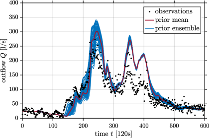
(a) Prior predictions.

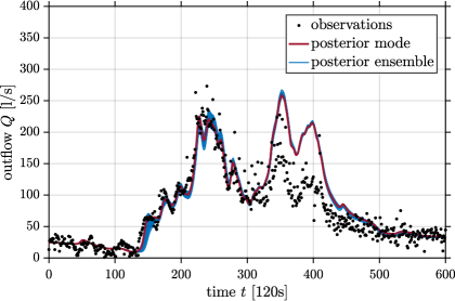
(b) Posterior predictions.

Figure 9: Stochastic model predictions. Ensembles of predictions pertaining to the prior and posterior mode are shown in Figs. 9 and 9, respectively. As already seen in Fig. 2, pronounced discrepancies between the predicted and observed outflow are found in the time intervals $[150,200]$ and $[250,500]$.

We now investigate how well the posterior mode of $\pi_{2}(\bm{x},\bm{b},\sigma,\tau\>\!|\>\!\bm{y})$ aligns with the data. The mode estimate of the discrepancy function $\hat{\delta}(t)=\delta(\hat{\bm{b}},t)$ is plotted in Fig. 10. It indicates a trend that the model underpredicts the actual rainfall in roughly the interval $t/120\,\mathrm{s}\in[100,250]$ and overpredicts in $t/120\,\mathrm{s}\in[250,500]$. These mis-predictions occur more or less for the period $t/120\,\mathrm{s}\in[100,450]$ of the precipitation event that was shown in Fig. 2. At the boundaries, say for $t/120\,\mathrm{s}\in[0,100]$ and $t/120\,\mathrm{s}\in[500,600]$, the discrepancy vanishes as far as the low-degree polynomial representation admits. The accordingly corrected predictions $\hat{\mathcal{M}}_{p}(\hat{\bm{x}})+\hat{\bm{\delta}}$ are depicted in Fig. 11. They align with the data reasonably well. One, two and three $\hat{\sigma}$ prediction intervals are added so as to visualize the posterior mode prediction uncertainty.

While the learned discrepancy term effectively captures the model errors as a function of time, it is again noted that its specific form in Fig. 10 pertains to the model and the studied rainfall event, i.e. it does not generalize to unseen events. The procedure, however, of separating and representing random noise and systematic error can be applied more generally. It is further remarked that, due to the additive and symmetric noise model, the prediction intervals in Fig. 11 extend to negative outflow values. Since these values are physically nonsensical, they shall be ignored.

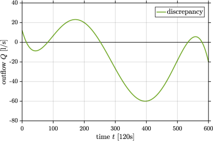
Figure 10: Model discrepancy. The posterior mode reveals the bias of the simulator, especially in the time intervals $[150,200]$ and $[250,500]$, where mispredictions of the outflow occurred in Fig. 2.

Figure 11: Corrected predictions. Incorporating the bias identified in Fig. 10 and the level of random errors corresponding to the posterior mode in Fig. 8 leads to well-calibrated predictions and uncertainty envelopes.

5 Discussion and conclusion

An efficient method for the non-intrusive emulation of time-dependent hydrological systems was presented in this paper. The idea was to exploit typical characteristics of the system response based on principal component analysis and sparse polynomial chaos expansions. First of all, the dimensionality of the output space was reduced by means of principal component analysis. This takes advantage of a linear correlation of the different response quantities. Following this, the reduced outputs were represented as polynomial chaos expansions. This enabled the utilization of sparsity patterns in the basis decompositions. All in all, a very fast and accurate emulator was constructed this way.

The availability of a fast metamodel facilitated the probabilistic uncertainty quantification of an urban drainage simulator. Variance-based global sensitivity analysis and computational Bayesian inference were accomplished for the dynamical simulation of a small catchment area. It was shown how the Sobol’ indices of the predicted outflow at various time instants can be efficiently computed based on the polynomial expansions of the principal components. The calibration of the unknown hydrological parameters, random measurement uncertainties and systematic model errors through Markov chain Monte Carlo sampling was made possible. In this context, a significant speedup was achieved through the substitution of the original simulator with the developed surrogate model.

After all, it has to be said that the problem studied was rather simple. While the catchment area under study had multiple outlets, only a single one at the wastewater treatment plant was considered. A very coarse-grained parametrization of the unknowns based on crude averages over hundreds of sub-catchments and channels was used. Besides, the whole case study was dependent on a single precipitation event for which the rainfall record was taken as if it were measured without error. It is therefore envisaged to address more complex and realistic problems in the future. This may include problems that feature a finer-grained representation of the spatially dependent input parameters and their uncertainties, and models that explicitly acknowledge errors in the rainfall input data. This may also include the analysis of various different precipitation events and longer time series data. The resulting increase of the input and output dimensionality can be coped with on the basis of the proposed technique for structure-exploiting surrogate modeling.

Software availability

The urban drainage simulator was implemented with the storm water management model (SWMM) [64]. For further details the reader is redirected to the website https://www.epa.gov/water-research/storm-water-management-model-swmm. A metamodel based on principal component analysis and polynomial chaos expansions was computed with UQLab [82, 83], a Matlab-based framework for uncertainty quantification (UQ). The software is free for academic use and can be obtained from http://www.uqlab.com/.

Appendix A Principal component analysis

Consider the random vector $\tilde{\bm{Y}}$ with mean $\bm{\mu}_{\tilde{\bm{Y}}}=\mathds{E}[\tilde{\bm{Y}}]$ and covariance matrix $\bm{\Sigma}_{\tilde{\bm{Y}}}=\mathrm{Cov}[\tilde{\bm{Y}}]=\mathds{E}[(\tilde{\bm{Y}}-\bm{\mu}_{\tilde{\bm{Y}}})(\tilde{\bm{Y}}-\bm{\mu}_{\tilde{\bm{Y}}})^{\top}]$. Since $\bm{\Sigma}_{\tilde{\bm{Y}}}$ is symmetric and positive definite, one can find linearly independent eigenvectors $\bm{\phi}_{i}$ with positive eigenvalues $\lambda_{i}>0$ for $i=0,\ldots,N$. The characteristic vectors and values satisfy

$$\bm{\Sigma}_{\tilde{\bm{Y}}}\bm{\phi}_{i}=\lambda_{i}\bm{\phi}_{i}.$$ (30)

Eigenvectors corresponding to distinct eigenvalues are orthogonal anyway, while they can be always chosen as such for degenerate eigenvalues. We assume that the eigenvalues are arranged in decreasing order $\lambda_{0}\geq\lambda_{1}\geq\ldots\geq\lambda_{N}$ and that eigenvectors are normalized such that $\bm{\phi}_{i}^{\top}\bm{\phi}_{j}=\delta_{ij}$ for $i,j=0,\ldots,N$. Leaving degeneracy aside, this way the eigenvectors are uniquely defined up to a multiplication by $-1$.

The set of eigenvectors constitutes an orthonormal basis of $\mathds{R}^{N+1}=\mathrm{span}(\{\bm{\phi}_{i}\}_{i=0}^{N})$. One can define the orthogonal matrix $\bm{\Phi}=(\bm{\phi}_{0},\bm{\phi}_{1},\ldots,\bm{\phi}_{N})$ with $\bm{\Phi}^{\top}\bm{\Phi}=\bm{\Phi}\bm{\Phi}^{\top}=\bm{I}$. It diagonalizes the covariance matrix by

$$\bm{\Phi}^{\top}\bm{\Sigma}_{\tilde{\bm{Y}}}\bm{\Phi}=\bm{\Lambda}=\begin{pmatrix}\lambda_{0}&0&\ldots&0\\ 0&\lambda_{1}&\ldots&0\\ \vdots&\vdots&\ddots&\vdots\\ 0&0&\ldots&\lambda_{N}\\ \end{pmatrix}.$$ (31)

Vice versa, one obtains the spectral eigendecomposition of the covariance matrix $\bm{\Sigma}_{\tilde{\bm{Y}}}=\bm{\Phi}\bm{\Lambda}\bm{\Phi}^{\top}=\sum_{i=0}^{N}\lambda_{i}\bm{\phi}_{i}\bm{\phi}_{i}^{\top}$. Now consider the orthogonal transformation

$$\tilde{\bm{Z}}=\bm{\Phi}^{\top}(\tilde{\bm{Y}}-\bm{\mu}_{\tilde{\bm{Y}}}).$$ (32)

The linearly transformed random vector has mean zero $\mathds{E}[\tilde{\bm{Z}}]=\bm{0}$ and the diagonal covariance matrix $\mathrm{Cov}[\tilde{\bm{Z}}]=\mathds{E}[\tilde{\bm{Z}}\tilde{\bm{Z}}^{\top}]=\bm{\Lambda}$, i.e. it has been centered and decorrelated. Independence is not necessarily implied thereby. Though, the special case involving Gaussianity forms an exception. The back-transformation reads

$$\tilde{\bm{Y}}=\bm{\mu}_{\tilde{\bm{Y}}}+\bm{\Phi}\tilde{\bm{Z}}=\bm{\mu}_{\tilde{\bm{Y}}}+\sum\limits_{i=0}^{N}\tilde{Z}_{i}\bm{\phi}_{i}.$$ (33)

This is the discrete KL expansion of the random vector $\tilde{\bm{Y}}$. The random variables $\tilde{Z}_{i}=\bm{\phi}_{i}^{\top}(\tilde{\bm{Y}}-\bm{\mu}_{\tilde{\bm{Y}}})$ for $i=0,\ldots,N$ are called the principal components.

Define the total variance of $\tilde{\bm{Y}}$ as the sum $\sum_{i=0}^{N}\mathrm{Var}[\tilde{Y}_{i}]$ of the individual variances of $\tilde{Y}_{i}$. The orthogonal transformation preserves the total variance in the sense that

$$\sum_{i=0}^{N}\mathrm{Var}[\tilde{Y}_{i}]=\operatorname{tr}(\bm{\Sigma}_{\tilde{\bm{Y}}})=\operatorname{tr}(\bm{\Lambda})=\sum_{i=0}^{N}\mathrm{Var}[\tilde{Z}_{i}]=\sum_{i=0}^{N}\lambda_{i}.$$ (34)

This follows from the invariance of the trace under cyclic permutations. The KL expansion is optimal with respect to compaction of the total variance. Consider keeping only the first $N^{\prime}+1\leq N+1$ terms in

$$\tilde{\bm{Y}}\approx\bm{\mu}_{\tilde{\bm{Y}}}+\sum\limits_{i=0}^{N^{\prime}}\tilde{Z}_{i}\bm{\phi}_{i}.$$ (35)

This is the expansion that contains most of the total variance with $N^{\prime}+1$ terms only. The number of terms is normally chosen such that at least a predetermined fraction $\sum_{i=0}^{N^{\prime}}\lambda_{i}/\sum_{i=0}^{N}\lambda_{i}$ of the total variance is explained.

References

- [1] R. C. Smith. Uncertainty Quantification: Theory, Implementation, and Applications. Computational Science and Engineering. Society for Industrial and Applied Mathematics (SIAM), Philadelphia, Pennsylvania, USA, 2014.
- [2] C. Soize. Uncertainty Quantification: An Accelerated Course with Advanced Applications in Computational Engineering. Number 47 in Interdisciplinary Applied Mathematics. Springer International Publishing AG, Cham, Switzerland, 2017.
- [3] H. Bijl, D. Lucor, S. Mishra, and C. Schwab, editors. Uncertainty Quantification in Computational Fluid Dynamics. Number 92 in Lecture Notes in Computational Science and Engineering. Springer International Publishing, Cham, Switzerland, 2013.
- [4] S. Sarkar and J. A. S. Witteveen, editors. Uncertainty Quantification in Computational Science: Theory and Application in Fluids and Structural Mechanics. World Scientific Publishing Co. Pte. Ltd., Singapore, 2017.
- [5] K. Beven. Environmental Modelling: An Uncertain Future? Routledge, Abingdon, Oxfordshire, UK, 2009.
- [6] K. Beven. Rainfall-Runoff Modelling: The Primer. Wiley-Blackwell, Chichester, West Sussex, UK, 2 edition, 2012.
- [7] J. C. Refsgaard, J. P. van der Sluijs, A. L. Højberg, and P. A. Vanrolleghem. Uncertainty in the environmental modelling process – A framework and guidance. Environ. Modell. Software, 22(11):1543–1556, 2007.
- [8] A. Deletic, C. B. S. Dotto, D. T. McCarthy, M. Kleidorfer, G. Freni, G. Mannina, M. Uhl, M. Henrichs, T. D. Fletcher, W. Rauch, J. L. Bertrand-Krajewski, and S. Tait. Assessing uncertainties in urban drainage models. Phys. Chem. Earth., 42–44:3–10, 2012.
- [9] C. M. DeChant and H. Moradkhani. Hydrologic prediction and uncertainty quantification. In S. Eslamian, editor, Handbook of Engineering Hydrology: Modeling, Climate Change, and Variability, chapter 20, pages 387–414. CRC Press, Boca Raton, Florida, USA, 2014.
- [10] J. C. Ascough, H. R. Maier, J. K. Ravalico, and M. W. Strudley. Future research challenges for incorporation of uncertainty in environmental and ecological decision-making. Ecol. Modell., 219(3–4):383–399, 2008.
- [11] L. Uusitalo, A. Lehikoinen, I. Helle, and K. Myrberg. An overview of methods to evaluate uncertainty of deterministic models in decision support. Environ. Modell. Software, 63:24–31, 2015.
- [12] L. García, J. Barreiro-Gomez, E. Escobar, D. Téllez, N. Quijano, and C. Ocampo-Martinez. Modeling and real-time control of urban drainage systems: A review. Adv. Water Resour., 85:120–132, 2015.
- [13] B. M. Ayyub. Elicitation of Expert Opinions for Uncertainty and Risks. CRC Press, Boca Raton, Florida, USA, 2001.
- [14] A. O’Hagan, C. E. Buck, A. Daneshkhah, J. R. Eiser, P. H. Garthwaite, D. J. Jenkinson, J. E. Oakley, and T. Rakow. Uncertain Judgements: Eliciting Experts’ Probabilities. Statistics in Practice. John Wiley & Sons, Ltd., Chichester, West Sussex, UK, 2006.
- [15] J. Lei and W. Schilling. Parameter uncertainty propagation analysis for urban rainfall runoff modelling. Water Sci. Technol., 29(1–2):145–154, 1994.
- [16] S. Gabellani, G. Boni, L. Ferraris, J. von Hardenberg, and A. Provenzale. Propagation of uncertainty from rainfall to runoff: A case study with a stochastic rainfall generator. Adv. Water Resour., 30(10):2061–2071, 2007.
- [17] G. Baroni and S. Tarantola. A general probabilistic framework for uncertainty and global sensitivity analysis of deterministic models: A hydrological case study. Environ. Modell. Software, 51:26–34, 2014.
- [18] F. Pianosi, K. Beven, J. Freer, J. W. Hall, J. Rougier, D. B. Stephenson, and T. Wagener. Sensitivity analysis of environmental models: A systematic review with practical workflow. Environ. Modell. Software, 79:214–232, 2016.
- [19] D. Huard and A. Mailhot. A Bayesian perspective on input uncertainty in model calibration: Application to hydrological model “abc”. Water Resour. Res., 42(7):1–14, 2006.
- [20] W. Fernandes and A. T. Silva. Introduction to Bayesian analysis of hydrologic variables. In M. Naghettini, editor, Fundamentals of Statistical Hydrology, chapter 11, pages 497–536. Springer International Publishing, Cham, Switzerland, 2017.
- [21] S. H. Lee and W. Chen. A comparative study of uncertainty propagation methods for black-box-type problems. Struct. Multidiscip. Optim., 37(3):239–253, 2009.
- [22] M. Arnst and J.-P. Ponthot. An overview of nonintrusive characterization, propagation, and sensitivity analysis of uncertainties in computational mechanics. Int. J. Uncertainty Quantification, 4(5):387–421, 2014.
- [23] J. C. Helton, J. D. Johnson, C. J. Sallaberry, and C. B. Storlie. Survey of sampling-based methods for uncertainty and sensitivity analysis. Reliab. Eng. Syst. Saf., 91(10–11):1175–1209, 2006.
- [24] A. Saltelli, S. Tarantola, F. Campolongo, and M. Ratto. Sensitivity Analysis in Practice: A Guide to Assessing Scientific Models. John Wiley & Sons, Ltd., Chichester, West Sussex, UK, 2004.
- [25] A. Saltelli, M. Ratto, T. Andres, F. Campolongo, J. Cariboni, D. Gatelli, M. Saisana, and S. Tarantola. Global Sensitivity Analysis: The Primer. John Wiley & Sons, Ltd., Chichester, West Sussex, UK, 2008.
- [26] B. Iooss and P. Lemaître. A review on global sensitivity analysis methods. In G. Dellino and C. Meloni, editors, Uncertainty Management in Simulation-Optimization of Complex Systems: Algorithms and Applications, number 59 in Operations Research/Computer Science Interfaces Series, pages 101–122. Springer, New York, 2015.
- [27] C. Prieur and S. Tarantola. Variance-based sensitivity analysis: Theory and estimation algorithms. In R. Ghanem, D. Higdon, and H. Owhadi, editors, Handbook of Uncertainty Quantification, chapter 35, pages 1217–1239. Springer International Publishing, Cham, Switzerland, 2017.
- [28] J. B. Nagel and B. Sudret. Bayesian multilevel model calibration for inverse problems under uncertainty with perfect data. J. Aerosp. Inf. Syst., 12(1):97–113, 2015.
- [29] J. B. Nagel and B. Sudret. A unified framework for multilevel uncertainty quantification in Bayesian inverse problems. Probab. Eng. Mech., 43:68–84, 2016.
- [30] M. C. Kennedy and A. O’Hagan. Bayesian calibration of computer models. J. R. Stat. Soc. Ser. B, 63(3):425–464, 2001.
- [31] J. Brynjarsdóttir and A. O’Hagan. Learning about physical parameters: the importance of model discrepancy. Inverse Prob., 30(11):1–24, 2014.
- [32] J. Beck and K. Yuen. Model selection using response measurements: Bayesian probabilistic approach. J. Eng. Mech., 130(2):192–203, 2004.
- [33] I. Park and R. V. Grandhi. Quantifying multiple types of uncertainty in physics-based simulation using Bayesian model averaging. AIAA J., 49(5):1038–1045, 2011.
- [34] C. P. Robert and G. Casella. Monte Carlo Statistical Methods. Springer Series in Statistics. Springer, New York, 2 edition, 2004.
- [35] R. Y. Rubinstein and D. P. Kroese. Simulation and the Monte Carlo Method. Wiley Series in Probability and Statistics. John Wiley & Sons, Inc., Hoboken, New Jersey, USA, 3 edition, 2017.
- [36] S. Duane, A. D. Kennedy, B. J. Pendleton, and D. Roweth. Hybrid Monte Carlo. Phys. Lett. B, 195(2):216–222, 1987.
- [37] M. Betancourt. A conceptual introduction to Hamiltonian Monte Carlo, 2017. arXiv:1701.02434.
- [38] P. Angelikopoulos, C. Papadimitriou, and P. Koumoutsakos. Bayesian uncertainty quantification and propagation in molecular dynamics simulations: A high performance computing framework. J. Chem. Phys., 137(14):1–19, 2012.
- [39] P. E. Hadjidoukas, P. Angelikopoulos, C. Papadimitriou, and P. Koumoutsakos. 4U: A high performance computing framework for Bayesian uncertainty quantification of complex models. J. Comput. Phys., 284:1–21, 2015.
- [40] I. M. Franck and P. S. Koutsourelakis. Sparse variational Bayesian approximations for nonlinear inverse problems: Applications in nonlinear elastography. Comput. Meth. Appl. Mech. Eng., 299:215–244, 2016.
- [41] I. M. Franck and P. S. Koutsourelakis. Multimodal, high-dimensional, model-based, Bayesian inverse problems with applications in biomechanics. J. Comput. Phys., 329:91–125, 2017.
- [42] T. A. El Moselhy and Y. M. Marzouk. Bayesian inference with optimal maps. J. Comput. Phys., 231(23):7815–7850, 2012.
- [43] M. Parno, T. Moselhy, and Y. Marzouk. A multiscale strategy for Bayesian inference using transport maps. SIAM/ASA J. Uncertainty Quantification, 4(1):1160–1190, 2016.
- [44] J. B. Nagel and B. Sudret. Spectral likelihood expansions for Bayesian inference. J. Comput. Phys., 309:267–294, 2016.
- [45] A. Schöniger, T. Wöhling, L. Samaniego, and W. Nowak. Model selection on solid ground: Rigorous comparison of nine ways to evaluate Bayesian model evidence. Water Resour. Res., 50(12):9484–9513, 2014.
- [46] P. Liu, A. S. Elshall, M. Ye, P. Beerli, X. Zeng, D. Lu, and Y. Tao. Evaluating marginal likelihood with thermodynamic integration method and comparison with several other numerical methods. Water Resour. Res., 52(2):734–758, 2016.
- [47] M. Ratto, A. Castelletti, and A. Pagano. Emulation techniques for the reduction and sensitivity analysis of complex environmental models. Environ. Modell. Software, 34:1–4, 2012.
- [48] A. Castelletti, S. Galelli, M. Ratto, R. Soncini-Sessa, and P. C. Young. A general framework for dynamic emulation modelling in environmental problems. Environ. Modell. Software, 34:5–18, 2012.
- [49] T. J. Santner, B. J. Williams, and W. I. Notz. The Design and Analysis of Computer Experiments. Springer Series in Statistics. Springer, New York, 2003.
- [50] C. E. Rasmussen and C. K. I. Williams. Gaussian Processes for Machine Learning. Adaptive Computation and Machine Learning. The MIT Press, Cambridge, Massachusetts, USA, 2006.
- [51] O. P. Le Maître and O. M. Knio. Spectral Methods for Uncertainty Quantification: With Applications to Computational Fluid Dynamics. Scientific Computation. Springer, Dordrecht, Netherlands, 2010.
- [52] D. Xiu. Numerical Methods for Stochastic Computations: A Spectral Method Approach. Princeton University Press, Princeton, New Jersey, USA, 2010.
- [53] G. Blatman and B. Sudret. Adaptive sparse polynomial chaos expansion based on least angle regression. J. Comput. Phys., 230(6):2345–2367, 2011.
- [54] J. D. Jakeman, M. S. Eldred, and K. Sargsyan. Enhancing -minimization estimates of polynomial chaos expansions using basis selection. J. Comput. Phys., 289:18–34, 2015.
- [55] J. Peng, J. Hampton, and A. Doostan. On polynomial chaos expansion via gradient-enhanced -minimization. J. Comput. Phys., 310:440–458, 2016.
- [56] K. Sargsyan, C. Safta, H. N. Najm, B. J. Debusschere, D. Ricciuto, and P. Thornton. Dimensionality reduction for complex models via Bayesian compressive sensing. Int. J. Uncertainty Quantification, 4(1):63–93, 2014.
- [57] G. Karagiannis, B. A. Konomi, and G. Lin. A Bayesian mixed shrinkage prior procedure for spatial–stochastic basis selection and evaluation of gPC expansions: Applications to elliptic SPDEs. J. Comput. Phys., 284:528–546, 2015.
- [58] Q. Shao, A. Younes, M. Fahs, and T. A. Mara. Bayesian sparse polynomial chaos expansion for global sensitivity analysis. Comput. Meth. Appl. Mech. Eng., 318:474–496, 2017.
- [59] V. P. Singh and D. A. Woolhiser. Mathematical modeling of watershed hydrology. J. Hydrol. Eng., 7(4):270–292, 2002.
- [60] E. Todini. History and perspectives of hydrological catchment modelling. Hydrol. Res., 42(2–3):73–85, 2011.
- [61] P. M. Bach, W. Rauch, P. S. Mikkelsen, D. T. McCarthy, and A. Deletic. A critical review of integrated urban water modelling – Urban drainage and beyond. Environ. Modell. Software, 54:88–107, 2014.
- [62] E. Salvadore, J. Bronders, and O. Batelaan. Hydrological modelling of urbanized catchments: A review and future directions. J. Hydrol., 529:62–81, 2015.
- [63] D. Machac. Mechanistic Emulators as Surrogates to Slow Hydrological Models. PhD thesis, Swiss Federal Institute of Technology (ETH Zürich), Zürich, Switzerland, 2015.
- [64] L. A. Rossman. Storm Water Management Model: User’s Manual. US EPA Office of Research and Development, Washington, D.C., USA, 2015.
- [65] D. Machac, P. Reichert, and C. Albert. Emulation of dynamic simulators with application to hydrology. J. Comput. Phys., 313:352–366, 2016.
- [66] J. P. Carbajal, J. P. Leitão, C. Albert, and J. Rieckermann. Appraisal of data-driven and mechanistic emulators of nonlinear simulators: The case of hydrodynamic urban drainage models. Environ. Modell. Software, 92:17–27, 2017.
- [67] D. Machac, P. Reichert, J. Rieckermann, and C. Albert. Fast mechanism-based emulator of a slow urban hydrodynamic drainage simulator. Environ. Modell. Software, 78:54–67, 2016.
- [68] P. Sochala and O. P. Le Maître. Polynomial chaos expansion for subsurface flows with uncertain soil parameters. Adv. Water Resour., 62:139–154, 2013.
- [69] Y. R. Fan, W. Huang, G. H. Huang, K. Huang, and X. Zhou. A PCM-based stochastic hydrological model for uncertainty quantification in watershed systems. Stochastic Environ. Res. Risk Assess., 29(3):915–927, 2015.
- [70] N. Fajraoui, T. A. Mara, A. Younes, and R. Bouhlila. Reactive transport parameter estimation and global sensitivity analysis using sparse polynomial chaos expansion. Water Air Soil Pollut., 223(7):4183–4197, 2012.
- [71] A. H. Elsheikh, I. Hoteit, and M. F. Wheeler. Efficient Bayesian inference of subsurface flow models using nested sampling and sparse polynomial chaos surrogates. Comput. Meth. Appl. Mech. Eng., 269:515–537, 2014.
- [72] M. D. McKay, R. J. Beckman, and W. J. Conover. A comparison of three methods for selecting values of input variables in the analysis of output from a computer code. Technometrics, 21(2):239–245, 1979.
- [73] I. T. Jolliffe. Principal Component Analysis. Springer Series in Statistics. Springer-Verlag, New York, 2 edition, 2002.
- [74] G. Blatman and B. Sudret. Principal component analysis and least angle regression in spectral stochastic finite element analysis. In M. H. Faber, J. Köhler, and K. Nishijima, editors, 11th International Conference on Applications of Statistics and Probability in Civil Engineering (ICASP11), chapter 82, pages 669–676. CRC Press/Balkema, Leiden, Netherlands, 2011.
- [75] G. Blatman and B. Sudret. Sparse polynomial chaos expansions of vector-valued response quantities. In G. Deodatis, B. R. Ellingwood, and D. M. Frangopol, editors, 11th International Conference on Structural Safety and Reliability (ICOSSAR 2013), chapter 434, pages 3245–3252. CRC Press/Balkema, Leiden, Netherlands, 2013.
- [76] M. Loève. Probability Theory. Number 45–46 in Graduate Texts in Mathematics. Springer-Verlag, New York, 4 edition, 1977–1978.
- [77] D. Xiu and G. E. Karniadakis. The Wiener–Askey polynomial chaos for stochastic differential equations. SIAM J. Sci. Comput., 24(2):619–644, 2002.
- [78] J. A. S. Witteveen, S. Sarkar, and H. Bijl. Modeling physical uncertainties in dynamic stall induced fluid–structure interaction of turbine blades using arbitrary polynomial chaos. Comput. Struct., 85(11–14):866–878, 2007.
- [79] D. Xiu. Stochastic collocation methods: A survey. In R. Ghanem, D. Higdon, and H. Owhadi, editors, Handbook of Uncertainty Quantification, chapter 20, pages 699–716. Springer International Publishing, Cham, Switzerland, 2017.
- [80] D. Vidaurre, C. Bielza, and P. Larrañaga. A survey of regression. Int. Stat. Rev., 81(3):361–387, 2013.
- [81] H. Zhang and R. H. Zamar. Least angle regression for model selection. Wiley Interdiscip. Rev. Comput. Stat., 6(2):116–123, 2014.
- [82] S. Marelli and B. Sudret. UQLab: A framework for uncertainty quantification in Matlab. In M. Beer, S.-K. Au, and J. W. Hall, editors, 2nd International Conference on Vulnerability, Uncertainty, and Risk: Quantification, Mitigation, and Management (ICVRAM-ISUMA 2014), chapter 257, pages 2554–2563. American Society of Civil Engineers (ASCE), Reston, Virginia, USA, 2014.
- [83] S. Marelli and B. Sudret. UQLab user manual – Polynomial Chaos Expansions. Chair of Risk, Safety & Uncertainty Quantification, ETH Zürich, 2018. Report # UQLab-V1.1-104.
- [84] G. Blatman and B. Sudret. An adaptive algorithm to build up sparse polynomial chaos expansions for stochastic finite element analysis. Probab. Eng. Mech., 25(2):183–197, 2010.
- [85] L. L. Gratiet, S. Marelli, and B. Sudret. Metamodel-based sensitivity analysis: Polynomial chaos expansions and Gaussian processes. In R. Ghanem, D. Higdon, and H. Owhadi, editors, Handbook of Uncertainty Quantification, chapter 38, pages 1289–1325. Springer International Publishing, Cham, Switzerland, 2017.
- [86] B. Sudret. Global sensitivity analysis using polynomial chaos expansions. Reliab. Eng. Syst. Saf., 93(7):964–979, 2008.
- [87] W. Hoeffding. A class of statistics with asymptotically normal distribution. Ann. Math. Stat., 19(3):293–325, 1948.
- [88] I. M. Sobol’. Sensitivity estimates for nonlinear mathematical models. Math. Model. Comput. Exp., 1(4):407–414, 1993.
- [89] H. Rabitz, Ö. F. Alış, J. Shorter, and K. Shim. Efficient input–output model representations. Comput. Phys. Commun., 117(1):11–20, 1999.
- [90] H. Rabitz and Ö. F. Alış. General foundations of high-dimensional model representations. J. Math. Chem., 25(2):197–233, 1999.
- [91] T. Homma and A. Saltelli. Importance measures in global sensitivity analysis of nonlinear models. Reliab. Eng. Syst. Saf., 52(1):1–17, 1996.
- [92] G. Li and H. Rabitz. General formulation of HDMR component functions with independent and correlated variables. J. Math. Chem., 50(1):99–130, 2012.
- [93] G. Chastaing, F. Gamboa, and C. Prieur. Generalized Hoeffding-Sobol decomposition for dependent variables - application to sensitivity analysis. Electron. J. Stat., 6:2420–2448, 2012.
- [94] J. E. Oakley and A. O’Hagan. Probabilistic sensitivity analysis of complex models: a Bayesian approach. J. R. Stat. Soc. Ser. B, 66(3):751–769, 2004.
- [95] F. Gamboa, A. Janon, T. Klein, and A. Lagnoux. Sensitivity indices for multivariate outputs. C. R. Mathematique, 351(7):307–310, 2013.
- [96] F. Gamboa, A. Janon, T. Klein, and A. Lagnoux. Sensitivity analysis for multidimensional and functional outputs. Electron. J. Stat., 8(1):575–603, 2014.
- [97] K. Campbell, M. D. McKay, and B. J. Williams. Sensitivity analysis when model outputs are functions. Reliab. Eng. Syst. Saf., 91(10–11):1468–1472, 2006.
- [98] O. Garcia-Cabrejo and A. Valocchi. Global sensitivity analysis for multivariate output using polynomial chaos expansion. Reliab. Eng. Syst. Saf., 126:25–36, 2014.
- [99] M. Lamboni, D. Makowski, S. Lehuger, B. Gabrielle, and H. Monod. Multivariate global sensitivity analysis for dynamic crop models. Field Crops Res., 113(3):312–320, 2009.
- [100] M. Lamboni, H. Monod, and D. Makowski. Multivariate sensitivity analysis to measure global contribution of input factors in dynamic models. Reliab. Eng. Syst. Saf., 96(4):450–459, 2011.
- [101] T. Sumner, E. Shephard, and I. D. L. Bogle. A methodology for global-sensitivity analysis of time-dependent outputs in systems biology modelling. J. R. Soc. Interface, 9(74):2156–2166, 2012.
- [102] J. Rohmer. Dynamic sensitivity analysis of long-running landslide models through basis set expansion and meta-modelling. Nat. Hazards, 73(1):5–22, 2014.
- [103] A. Marrel, B. Iooss, M. Jullien, B. Laurent, and E. Volkova. Global sensitivity analysis for models with spatially dependent outputs. Environmetrics, 22(3):383–397, 2011.
- [104] A. Marrel, N. Perot, and C. Mottet. Development of a surrogate model and sensitivity analysis for spatio-temporal numerical simulators. Stochastic Environ. Res. Risk Assess., 29(3):959–974, 2015.
- [105] I. M. Sobol’. Global sensitivity indices for nonlinear mathematical models and their Monte Carlo estimates. Math. Comput. Simul., 55(1–3):271–280, 2001.
- [106] I. Dimov and R. Georgieva. Monte Carlo algorithms for evaluating Sobol’ sensitivity indices. Math. Comput. Simul., 81(3):506–514, 2010.
- [107] D. Del Giudice, M. Honti, A. Scheidegger, C. Albert, P. Reichert, and J. Rieckermann. Improving uncertainty estimation in urban hydrological modeling by statistically describing bias. Hydrol. Earth Syst. Sci., 17(10):4209–4225, 2013.
- [108] D. Del Giudice, P. Reichert, V. Bareš, C. Albert, and J. Rieckermann. Model bias and complexity – Understanding the effects of structural deficits and input errors on runoff predictions. Environ. Modell. Software, 64:205–214, 2015.