Enumeration of Labelled and Unlabelled Hamiltonian Cycles
in Complete $k$-partite Graphs

Abstract

We enumerate labelled and unlabelled Hamiltonian cycles in complete $n$-partite graphs $K_{d,d,\ldots,d}$ having exactly $d$ vertices in each part (in other words, Turán graphs $T(nd,n))$. We obtain recurrence relations that allow us to find the exact values $b_{n}^{(d)}$ of such cycles for arbitrary $n$ and $d$.

Keywords: Hamiltonian cycles; Turán graphs; complete $n$-partite graphs; chord diagrams; linear diagrams; labelled and unlabelled enumeration.

1 Introduction

The problem of enumerating Hamiltonian cycles in different classes of graphs is one of the most difficult problems of enumerative combinatorics. Apart from some trivial examples (like Hamiltonian cycles in complete graphs), only a few exact results of this type are known. Due to the inherent complexity of such problems, the efforts of researchers have been largely concentrated on obtaining upper and lower bounds on the numbers of Hamiltonian cycles in different classes of graphs (see [1],[2],[3],[4],[5]). Even fewer results regarding unlabelled Hamiltonian cycles have been obtained so far.

Figure 1: A chord diagram

One exception in this regard is the work [6] in which the author derived an analytic formula for the numbers $H_{n}$ of labelled Hamiltonian cycles in $n$-dimensional octahedrons (http://oeis.org/A003436), that is, in $n$-partite graphs $K_{2,2,\ldots,2}$ having $2n$ vertices. That article also contains a table of the corresponding numbers for unlabelled Hamiltonian cycles, numerically computed for small $n$. 20 years later the numbers $H_{n}$ appeared once again in the problem of enumerating loopless chord diagrams [7]. A chord diagram consists of $2n$ points on a circle labelled with the numbers $1,2,\ldots,2n$ in a circular order and joined pairwise by chords (figure 1). A chord is said to be a loop if it connects two neighboring points (chord $\{1,2\}$ on Figure 1). A loopless chord diagram is a diagram without loops.

In the paper [8] a bijection between Hamiltonian paths in octahedrons and loopless chord diagrams was noted. Take an $n$-dimensional octahedron with a distinguished Hamiltonian cycle (Figure 2(a)) and draw it in such a way that this cycle forms a circle on a plane (Figure 2(b)). Then remove all of its edges that don’t belong to the Hamiltonian cycle and add chords between those vertices that weren’t connected by an edge before (Figure 2(c)). The resulting object is a chord diagram which is necessarily loopless: traversing a Hamiltonian cycle in $K_{2,2,\ldots,2}$ we can’t visit two vertices of the same part one after another. Clearly, this transformation is invertible.

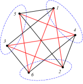
(a)

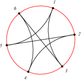
(b)

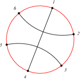
(c)

Figure 2: Correspondence between Hamiltonian cycles in octahedrons and chord diagrams

In the present work we extend this approach to a more general case of an $n$-partite graph $K_{d,d,\ldots,d}$, which has $d$ vertices in each part. Any Hamiltonian cycle in such graph can be represented by a generalized chord diagram built on $n\mathchar 8705\relax\nobreak d$ vertices (Figure 3). The class of such diagrams will be denoted as $B_{n}^{(d)}$. A generalized chord diagram consists of “chords” isomorphic to graphs $K_{d}$ connecting $d$ points of the diagram. Similarly to the special case $d\mathchar 12349\relax\nobreak 2$, in a loopless generalized chord diagram any pair of neighboring points must belong to two different chords.

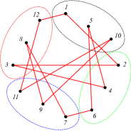
(a) Hamiltonian cycle in $K_{3,3,3,3}$

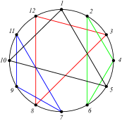
(b) Generalized chord diagram

Figure 3:

The first part of this paper is devoted to enumerating generalized loopless chord diagrams without considering symmetries or, equivalently, to enumerating labelled Hamiltonian cycles in $K_{d,d,\ldots,d}$. The approach is based on reduction $B_{n}^{(d)}$ to so-called linear diagrams $A_{n}^{(d)}$ [8]. Linear diagrams have a self-contained meaning; in particular, permutations in certain classes can be depicted as linear diagrams (see, for example, [9]).

Depending on the notion of isomorphism used, two diagrams are said to be isomorphic if one could be obtained from the other either by a rotation or by a combination of rotations and reflections of the circle. Isomorphism classes of labelled generalized chord diagrams are said to be unlabelled generalized chord diagrams. In the second part of the paper we derive a system of recurrence relations that can be used to efficiently compute the numbers of unlabelled diagrams, and hence enumerate unlabelled Hamiltonian cycles in the graphs $K_{d,d,\ldots,d}$. We provide answers for both notions of isomorphism: for rotations only, as well as for rotations and reflections.

2 Enumeration of labelled Hamiltonian cycles in $K_{d,d,\ldots,d}$

As we’ve noted before, it will be convenient to find the numbers $b_{n}^{(d)}$ of generalized loopless chord diagrams instead of doing that for Hamiltonian cycles in the graphs $K_{d,d,\ldots,d}$ directly (Figure 3 (b)).

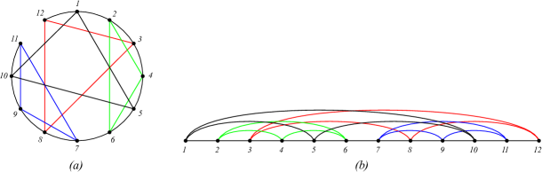
Figure 4: Cutting a triangle diagram

Each generalized chord diagram $B_{n}^{(d)}$ can be mapped to a unique linear diagram $A_{n}^{(d)}$ with $n\mathchar 8705\relax\nobreak d$ points (Figure 4) by cutting it (Figure 4 (a)) along the arc that connects the points $1$ and $n\mathchar 8705\relax\nobreak d$. The result is a loopless generalized linear diagram $A_{n}^{(d)}$ (Figure 4 (b)).

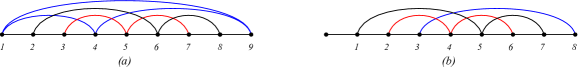
Figure 5:

Let $a_{n,k}^{(d)}$ be the number of generalized linear diagrams $A_{n}^{(d)}$ consisting of $d\mathchar 8705\relax\nobreak n$ points, $n$ complete subgraphs $K_{d}$ and having $k$ loops, $0\mathrel{\leqslant\nobreak}k\mathrel{\leqslant\nobreak}n(d\mathchar 8704\relax\nobreak 1)$. The numbers $b_{n}^{(d)}$ of generalized chord diagrams can be expressed through $a_{n,k}^{(d)}$ by the formula

$$b_{n}^{(d)}=a_{n,0}^{(d)}-\sum\limits_{k=0}^{d-2}{{d(n-1)-k-1}\choose{d-2-k}}a_{n-1,k}^{(d)}.$$ (1)

Indeed, among all $a_{n,0}^{(d)}$ generalized linear diagrams $A_{n,0}^{(d)}$ without loops we should retain only those that have no chord connecting two end vertices. Assume that after deleting such chord $K_{d}$ in a diagram that contains it, we obtain a linear diagram with $k$ loops. The number of ways to obtain a generalized linear diagram $A_{n,0}^{(d)}$ from an arbitrary linear diagram $A_{n\mathchar 8704\relax\nobreak 1,k}^{(d)}$ could be counted as follows. A diagram $A_{n\mathchar 8704\relax\nobreak 1,k}^{(d)}$ has exactly $d(n\mathchar 8704\relax\nobreak 1)\mathchar 8235\relax\nobreak 1$ positions to place the vertices of the new subgraph $K_{d}$. We must use the first and the last of these positions, among the remaining $(d\mathchar 8704\relax\nobreak 2)$ vertices of $K_{d}$ we must choose some $k$ to insert them into $k$ loops, and then distribute the remaining $d\mathchar 8704\relax\nobreak 2\mathchar 8704\relax\nobreak k$ vertices among $d(n\mathchar 8704\relax\nobreak 1)\mathchar 8704\relax\nobreak 1\mathchar 8704\relax\nobreak k$ positions. The latter could be done in ${{d(n\mathchar 8704\relax\nobreak 1)\mathchar 8704\relax\nobreak k\mathchar 8704\relax\nobreak 1}\choose{d\mathchar 8704\relax\nobreak 2\mathchar 8704\relax\nobreak k}}$ ways. Summing ${{d(n\mathchar 8704\relax\nobreak 1)\mathchar 8704\relax\nobreak k\mathchar 8704\relax\nobreak 1}\choose{d\mathchar 8704\relax\nobreak 2\mathchar 8704\relax\nobreak k}}a_{n\mathchar 8704\relax\nobreak 1,k}^{(d)}$ over all possible $k$ we obtain the total number of all diagrams $A_{n,0}^{(d)}$ which have a chord connecting the first and the last point.

To find the numbers $b_{n}^{(d)}$ using the formula (1) we need some recurrence relations for the numbers $a_{n,k}^{(d)}$, $k\mathchar 12349\relax\nobreak 0,\ldots,d\mathchar 8704\relax\nobreak 2$. It will be easier to start with some recurrence relations for a broader range of possible values of $k$. Namely, we claim that for $k\mathchar 12349\relax\nobreak 0,\ldots,n(d\mathchar 8704\relax\nobreak 1)$ the following is true:

$$a_{n,k}^{(d)}=\sum\limits_{t=k-d+1}^{k+d-1}{c_{n,k,t}^{(d)}\mathchar 8705\relax\nobreak a_{n-1,t}^{(d)}},\qquad n>0,\quad 0\mathrel{\leqslant\nobreak}k\mathrel{\leqslant\nobreak}n(d-1),$$ (2)

$$c_{n,k,t}^{(d)}=\sum\limits_{i=0}^{d-1}{{d-1}\choose i}{t\choose t+i-k}{{d(n-1)-t}\choose d-2i-t+k-1},$$ (3)

$$a_{0,0}^{(d)}\mathchar 12349\relax\nobreak 1,\qquad\qquad a_{n,k}^{(d)}\mathchar 12349\relax\nobreak 0\qquad\text{for $n\mathchar 12604\relax\nobreak 0$, $k\mathchar 12604\relax\nobreak 0$ and $k\mathchar 12606\relax\nobreak n(d\mathchar 8704\relax\nobreak 1)$}.$$

The proof of relations (2)–(3) is based on the procedure of removing the subgraph $K_{d}$ which contains the rightmost point of some generalized linear diagram $A_{n,k}^{(d)}$. Since removing $K_{d}$ adds or removes not more than $d\mathchar 8704\relax\nobreak 1$ loops, after removing it from some diagram $A_{n,k}^{(d)}$ we obtain a generalized linear diagram $A_{n\mathchar 8704\relax\nobreak 1,t}^{(d)}$ with $t$ loops, $t\mathrel{\mathchar 8754\relax\nobreak}[k\mathchar 8704\relax\nobreak(d\mathchar 8704\relax\nobreak 1),k\mathchar 8235\relax\nobreak(d\mathchar 8704\relax\nobreak 1)]$.

Figure 6: Generalized linear diagram $A_{3,8}^{(6)}$

As an example on Figure 6 we show a generalized linear diagram $A_{n,k}^{(d)}$ for $n\mathchar 12349\relax\nobreak 3$, $d\mathchar 12349\relax\nobreak 6$ and $k\mathchar 12349\relax\nobreak 8$. Removing the subgraph $K_{6}$ that contains its rightmost point $18$ yields a generalized linear diagram $A_{2,6}^{(6)}$.

Now assume that we are given a diagram $A_{n\mathchar 8704\relax\nobreak 1,t}^{(d)}$. The number of ways to transform it into a diagram $A_{n,k}^{(d)}$ by adding a subgraph $K_{d}$ which would contain its rightmost point could be counted as follows. Denote by $i$ the number of loops formed by neighboring vertices of $K_{d}$ after adding it to $A_{n\mathchar 8704\relax\nobreak 1,t}^{(d)}$ ($i\mathchar 12349\relax\nobreak 3$ for the subgraph $K_{5}$, depicted on Figure 6). For the diagram $A_{n,k}^{(d)}$ to have exactly $k$ loops after adding $K_{d}$, this subgraph $K_{d}$ must destroy $t\mathchar 8235\relax\nobreak i\mathchar 8704\relax\nobreak k$ existing loops ($t\mathchar 8235\relax\nobreak i\mathchar 8704\relax\nobreak k\mathchar 12349\relax\nobreak 1$ for the diagram $A_{2,6}^{(6)}$) by its vertices placed under these loops. Finally we have $d(n\mathchar 8704\relax\nobreak 1)\mathchar 8704\relax\nobreak t$ remaining positions among which we can distribute $d\mathchar 8704\relax\nobreak i\mathchar 8704\relax\nobreak 1\mathchar 8704\relax\nobreak(t\mathchar 8235\relax\nobreak i\mathchar 8704\relax\nobreak k)$ remaining vertices of the subgraph $K_{d}$ ($6$ positions for the only vertex for the example shown on Figure 6). Counting the total number of ways to perform these combinatorial actions, we prove the formulas (2) – (3).

Note the following special cases for the relations (1)–(3). For $d\mathchar 12349\relax\nobreak 2$ the formula (1) becomes the formula (LABEL:eq:dd_b_nk), and the formulas (2)–(3) become (LABEL:eq:dd_a_nk). For $d\mathchar 12349\relax\nobreak 3$ the expression for $b_{n}^{(3)}$ takes the form

$$b_{n}^{(3)}\mathchar 12349\relax\nobreak a_{n,0}\mathchar 8704\relax\nobreak(3n\mathchar 8704\relax\nobreak 4)a_{n\mathchar 8704\relax\nobreak 1,0}^{(3)}\mathchar 8235\relax\nobreak a_{n\mathchar 8704\relax\nobreak 1,1}^{(3)},$$

and the system (2)–(3) gets simplified to

$$a_{n,k}\mathchar 12349\relax\nobreak a_{n\mathchar 8704\relax\nobreak 1,k\mathchar 8704\relax\nobreak 2}\mathchar 8235\relax\nobreak 2\,[3(n\mathchar 8704\relax\nobreak 1)\mathchar 8704\relax\nobreak(k\mathchar 8704\relax\nobreak 1)]\,a_{n\mathchar 8704\relax\nobreak 1,k\mathchar 8704\relax\nobreak 1}\mathchar 8235\relax\nobreak\left[{{3(n\mathchar 8704\relax\nobreak 1)\mathchar 8704\relax\nobreak k}\choose{2}}\mathchar 8235\relax\nobreak 2k\right]a_{n\mathchar 8704\relax\nobreak 1,k}\mathchar 8235\relax\nobreak$$

$$\mathchar 8235\relax\nobreak(k\mathchar 8235\relax\nobreak 1)\,[3(n\mathchar 8704\relax\nobreak 1)\mathchar 8704\relax\nobreak(k\mathchar 8235\relax\nobreak 1)]\,a_{n\mathchar 8704\relax\nobreak 1,k\mathchar 8235\relax\nobreak 1}\mathchar 8235\relax\nobreak{{k\mathchar 8235\relax\nobreak 2}\choose{2}}a_{n\mathchar 8704\relax\nobreak 1,k\mathchar 8235\relax\nobreak 2}.$$

3 A closed system of recurrence relations for $a_{n,k}^{(d)}$, $k\mathchar 12349\relax\nobreak 0,\ldots,d\mathchar 8704\relax\nobreak 1$

The recurrence relations (2)–(3) in principle allow us to obtain the values of $a_{n,i}^{(d)}$, $i\mathchar 12349\relax\nobreak 0,\ldots,d\mathchar 8704\relax\nobreak 2$ that are sufficient for finding $b_{n}^{(d)}$. However, from the computational point of view this approach could be improved; ideally we would find a system of recurrences involving only those values of $a_{n,k}^{(d)}$ that explicitly appear in (1). For $d\mathchar 12349\relax\nobreak 2$ the approach described in [8] was to rewrite the system (2)–(3) as a system of recurrence relations, find the generating function $w(z,t)$ for $a_{n,k}$ and then substitute $z\mathchar 12349\relax\nobreak 0$ into it. The generating function $\varphi(t)\mathchar 12349\relax\nobreak w(z,0)$ obtained as a result of substitution defines the numbers $a_{n,0}^{(2)}\mathrel{\mathchar 8721\relax\nobreak}a_{n}^{(2)}$ sufficient for calculating $b_{n}^{(2)}$. Unfortunately this approach does not generalize well for $d\mathchar 12606\relax\nobreak 2$. One alternative approach would be to derive the corresponding system by a combinatorial argument. This approach works perfectly for $d\mathchar 12349\relax\nobreak 2$ (see [7],[8]), but even for $d\mathchar 12349\relax\nobreak 3$ an analogous combinatorial proof becomes quite cumbersome, and for $d\mathchar 12606\relax\nobreak 3$ the problem becomes practically intractable.

In turns out that we can actually use a combined approach: use combinatorial arguments together with the already obtained system of recurrence relations (2)–(3) for the numbers $a_{n,k}^{(d)}$. With this approach we can obtain a closed system for the sequences $a_{n,k}^{(d)}$, $k\mathchar 12349\relax\nobreak 0,\ldots,d\mathchar 8704\relax\nobreak 1$, the number of which exceeds the number of terms $a_{n,k}^{(d)}$ in the formula (1) by just one. Namely, substituting $k\mathchar 12349\relax\nobreak 0$ into the formula (2) we obtain the recurrence relation

$$a_{n,0}^{(d)}=\sum\limits_{t=0}^{d-1}{c_{n,0,t}^{(d)}\mathchar 8705\relax\nobreak a_{n-1,t}^{(d)}}.$$ (4)

Figure 7: Generalized linear diagram $A_{3,2}^{(5)}$

Figure 8: Reduced linear diagram

Figure 9: Generalized linear diagram $A_{2,2}^{(5)}$

For the values of $k$ from $1$ to $d\mathchar 8704\relax\nobreak 1$ the relations for $a_{n,k}^{(d)}$ could be obtained using combinatorial arguments. Namely, consider a generalized linear diagram $A_{n,k}^{(d)}$ that has $k$ loops distributed over $l$ subgraphs isomorphic to $K_{d}$, $1\mathrel{\leqslant\nobreak}l\mathrel{\leqslant\nobreak}k\mathchar 12604\relax\nobreak d$. We will begin with the simplest case $l\mathchar 12349\relax\nobreak 1$ for which all $k$ loops are formed by a single subgraph $K_{d}$ (Figure 7, the corresponding subgraph $K_{3}$ is shown in blue).

Contracting the loops, we transform $K_{d}$ into a subgraph $K_{d\mathchar 8704\relax\nobreak k}$ in a reduced diagram which is now loopless (Figure 8). After removing this subgraph we obtain a generalized linear diagram $A_{n\mathchar 8704\relax\nobreak 1,m}^{(d)}$ with $m$ loops, $0\mathrel{\leqslant\nobreak}m\mathrel{\leqslant\nobreak}d\mathchar 8704\relax\nobreak k$ (Figure 9, case $m\mathchar 12349\relax\nobreak 2$). Conversely, take any diagram $A_{n\mathchar 8704\relax\nobreak 1,m}^{(d)}$ and add a vertex of some new subgraph $K_{d\mathchar 8704\relax\nobreak k}$ under $m$ of its loops. The remaining $d\mathchar 8704\relax\nobreak k\mathchar 8704\relax\nobreak m$ vertices of the subgraph $K_{d\mathchar 8704\relax\nobreak k}$ should be distributed among $d(n\mathchar 8704\relax\nobreak 1)\mathchar 8235\relax\nobreak 1\mathchar 8704\relax\nobreak m$ possible positions in ${{d(n\mathchar 8704\relax\nobreak 1)\mathchar 8235\relax\nobreak 1\mathchar 8704\relax\nobreak m}\choose{d\mathchar 8704\relax\nobreak k\mathchar 8704\relax\nobreak m}}$ ways. Finally, $d\mathchar 8704\relax\nobreak k$ vertices of the subgraph $K_{d\mathchar 8704\relax\nobreak k}$ should be transformed into a subgraph $K_{d}$ by replacing $k$ of its vertices with loops of the diagram. This could be done in $\left(\!\!{{d\mathchar 8704\relax\nobreak k}\choose{k}}\!\!\right)\mathchar 12349\relax\nobreak{{d\mathchar 8704\relax\nobreak 1}\choose{k}}$ ways. Summing over $m$ from $0$ to $d\mathchar 8704\relax\nobreak k$, we obtain that for $l\mathchar 12349\relax\nobreak 1$ the numbers $a_{n,k,l\mathchar 12349\relax\nobreak 1}^{(d)}$ can be expressed as

$$a_{n,k,l=1}^{(d)}={{d-1}\choose{k}}\sum\limits_{m=0}^{d-k}{{d(n-1)+1-m}\choose{d-k-m}}a_{n-1,m}^{(d)},\qquad\qquad k=1,\ldots,d-1.$$ (5)

Figure 10: Generalized linear diagram $A_{4,3}^{(5)}$

For $l\mathchar 12606\relax\nobreak 1$ an analogous consideration becomes slightly more complicated. Indeed, let $d\mathchar 8704\relax\nobreak r_{i}$, $i\mathchar 12349\relax\nobreak 1,\ldots,l$ be the number of loops in a diagram $A_{n,k}^{(d)}$ which belong to the $i$-th subgraph $K_{d}$, and let

$$\sum_{i=1}^{l}(d-r_{i})=k,\qquad 1\mathrel{\leqslant\nobreak}r_{1}\mathrel{\leqslant\nobreak}r_{2}\mathrel{\leqslant\nobreak}\ldots\mathrel{\leqslant\nobreak}r_{l}$$ (6)

(see a diagram $A_{4,3}^{(5)}$ with $l\mathchar 12349\relax\nobreak 2$, $r_{1}\mathchar 12349\relax\nobreak 3$, $r_{2}\mathchar 12349\relax\nobreak 4$ on Figure 10).

Figure 11: Reduced linear diagram

Contracting each such loop into a point, we obtain a reduced linear diagram with $n\mathchar 8704\relax\nobreak l$ subgraphs $K_{d}$, and $l$ subgraphs $K_{r_{i}}$ (Figure 11).

Figure 12: Generalized linear diagram $A_{2,4}^{(5)}$

Assume that after deleting the subgraphs $K_{r_{i}}$ we obtain a generalized linear diagram $A_{n\mathchar 8704\relax\nobreak l,m}^{(d)}$, $m\mathchar 12349\relax\nobreak 0,\ldots,ld\mathchar 8704\relax\nobreak k$ (see Figure 12 corresponding to the diagram $A_{2,4}^{(5)}$). We need to determine how many diagrams $A_{n,k}^{(d)}$ with $k$ loops distributed among $l$ subgraphs $K_{r_{i}}$ could be obtained from this diagram $A_{n\mathchar 8704\relax\nobreak l,m}^{(d)}$.

Figure 13: Generalized linear diagram $A_{2,4}^{(5)}$ with a subgraph $K_{r_{1}}$ added

Consider a diagram $A_{n\mathchar 8704\relax\nobreak l,m_{1}}^{(d)}$, $m_{1}\mathrel{\mathchar 8721\relax\nobreak}m$ and add a subgraph $K_{r_{1}}$ to it (Figure 13). Some of the existing loops may be destroyed by the vertices of $K_{r_{1}}$. An the same time the new diagram may have additional loops formed by neighboring vertices of the subgraph $K_{r_{1}}$. Denote by $s_{1}$ the number of loops destroyed by $K_{r_{1}}$, and by $j_{1}$ the number of loops formed by the vertices of $K_{r_{1}}$ ($s_{1}\mathchar 12349\relax\nobreak 2$, $j_{1}\mathchar 12349\relax\nobreak 1$ for the diagram shown on Figure 13).

Figure 14: A generalized linear diagram $A_{2,4}^{(5)}$ with an added reduced subgraph $K_{t_{1}}$

Consider instead of $K_{r_{1}}$ some other subgraph $K_{t_{1}}$, $t_{1}\mathchar 12349\relax\nobreak r_{1}\mathchar 8704\relax\nobreak j_{1}$ obtained by contracting $j_{1}$ loops of the subgraph $K_{r_{1}}$ (Figure 14). This subgraph $K_{t_{1}}$ could be placed into the original diagram $A_{n\mathchar 8704\relax\nobreak l,m_{1}}^{(d)}$ in such a way that $s_{1}$ vertices of the subgraph $K_{t_{1}}$ split the loops of the diagram $A_{n\mathchar 8704\relax\nobreak l,m_{1}}^{(d)}$ and the remaining $t_{1}\mathchar 8704\relax\nobreak s_{1}$ vertices are distributed among $v_{1}\mathchar 8704\relax\nobreak m_{1}$ positions free of loops, $v_{1}:\mathchar 12349\relax\nobreak d(n\mathchar 8704\relax\nobreak l)\mathchar 8235\relax\nobreak 1$, in ${{m_{1}}\choose{s_{1}}}{{v_{1}\mathchar 8704\relax\nobreak m_{1}}\choose{t_{1}\mathchar 8704\relax\nobreak s_{1}}}$ ways. Splitting $t_{1}$ vertices of the subgraph $K_{t_{1}}$ into $r_{1}$ vertices such that the vertices of the obtained subgraph $K_{r_{1}}$ form $j_{1}$ additional loops could be done in $\left(\!\!{{t_{1}}\choose{j_{1}}}\!\!\right)\mathchar 12349\relax\nobreak\left(\!\!{{r_{1}\mathchar 8704\relax\nobreak j_{1}}\choose{j_{1}}}\!\!\right)\mathchar 12349\relax\nobreak{{r_{1}\mathchar 8704\relax\nobreak 1}\choose{j_{1}}}$ ways. The number

$${{m_{1}}\choose{s_{1}}}{{v_{1}\mathchar 8704\relax\nobreak m_{1}}\choose{r_{1}\mathchar 8704\relax\nobreak j_{1}\mathchar 8704\relax\nobreak s_{1}}}{{r_{1}\mathchar 8704\relax\nobreak 1}\choose{j_{1}}}$$

of ways obtained in the first step should be multiplied by the number

$${{m_{2}}\choose{s_{2}}}{{v_{2}\mathchar 8704\relax\nobreak m_{2}}\choose{r_{2}\mathchar 8704\relax\nobreak j_{2}\mathchar 8704\relax\nobreak s_{2}}}{{r_{2}\mathchar 8704\relax\nobreak 1}\choose{j_{2}}}$$

of ways to add a subgraph $K_{r_{2}}$ into $v_{2}:\mathchar 12349\relax\nobreak v_{1}\mathchar 8235\relax\nobreak r_{1}$ positions to destroy $s_{2}$ loops of the linear diagram with $m_{2}\mathchar 12349\relax\nobreak m_{1}\mathchar 8235\relax\nobreak j_{1}\mathchar 8704\relax\nobreak s_{1}$ loops and add $j_{2}$ loops.

Continuing this process further, we will reach the final step where we will need to add a subgraph $K_{r_{l}}$ to a linear diagram. This step is special because after this addition there must be no loops in the diagram: after adding $K_{r_{1}},\ldots,K_{r_{l}}$ we must obtain a loopless reduced linear diagram (see Figure 11). Consequently, in this final step we must destroy all loops obtained on the previous step (that is, set $m_{l}\mathchar 12349\relax\nobreak s_{l}$) and the subgraph $K_{r_{l}}$ should not form any loops itself (that is, $j_{l}\mathchar 12349\relax\nobreak 0$).

Taking that into account, one could obtain the following final formula for the numbers $a_{n,k}^{(d)}$ for $l\mathchar 12606\relax\nobreak 1$:

$$a_{n,k,l>1}^{(d)}=\sum\limits_{R}\dfrac{\alpha_{R}}{\beta_{1}!\mathchar 8705\relax\nobreak\ldots\mathchar 8705\relax\nobreak\beta_{d-1}!}\sum\limits_{m=0}^{ld-k}p_{n,R,m}\mathchar 8705\relax\nobreak a_{n-l,m}^{(d)}.$$ (7)

Here $R$ is an ordered multiset $\{r_{1},\ldots,r_{l}\}$ that satisfies the conditions (6), the outer summation runs over all such multisets $R$ that

$$p_{n,R,m}:\mathchar 12349\relax\nobreak\sum\limits_{j_{1}\mathchar 12349\relax\nobreak 0}^{r_{1}\mathchar 8704\relax\nobreak 1}\ldots\sum\limits_{j_{l\mathchar 8704\relax\nobreak 1}\mathchar 12349\relax\nobreak 0}^{r_{l\mathchar 8704\relax\nobreak 1}\mathchar 8704\relax\nobreak 1}\sum\limits_{s_{1}\mathchar 12349\relax\nobreak 0}^{\min\{m_{1},r_{1}\mathchar 8704\relax\nobreak j_{1}\}}\ldots\sum\limits_{s_{l\mathchar 8704\relax\nobreak 1}\mathchar 12349\relax\nobreak 0}^{\min\{m_{l\mathchar 8704\relax\nobreak 1},r_{l\mathchar 8704\relax\nobreak 1}\mathchar 8704\relax\nobreak j_{l\mathchar 8704\relax\nobreak 1}\}}\prod\limits_{i\mathchar 12349\relax\nobreak 1}^{l\mathchar 8704\relax\nobreak 1}{{m_{i}}\choose{s_{i}}}{{v_{i}\mathchar 8704\relax\nobreak m_{i}}\choose{r_{i}\mathchar 8704\relax\nobreak j_{i}\mathchar 8704\relax\nobreak s_{i}}}{{r_{i}\mathchar 8704\relax\nobreak 1}\choose{j_{i}}}{{v_{l}\mathchar 8704\relax\nobreak m_{l}}\choose{r_{l}\mathchar 8704\relax\nobreak m_{l}}},$$

$$m_{i\mathchar 8235\relax\nobreak 1}:\mathchar 12349\relax\nobreak m_{i}\mathchar 8235\relax\nobreak j_{i}\mathchar 8704\relax\nobreak s_{i},\quad v_{i\mathchar 8235\relax\nobreak 1}:\mathchar 12349\relax\nobreak v_{i}\mathchar 8235\relax\nobreak r_{i},\quad i\mathchar 12606\relax\nobreak 1;\qquad m_{1}:\mathchar 12349\relax\nobreak m,\quad v_{1}:\mathchar 12349\relax\nobreak d(n\mathchar 8704\relax\nobreak l)\mathchar 8235\relax\nobreak 1,$$

$$\alpha_{R}:\mathchar 12349\relax\nobreak\prod\limits_{i\mathchar 12349\relax\nobreak 1}^{l}\left(\!\!{{r_{i}}\choose{d\mathchar 8704\relax\nobreak r_{i}}}\!\!\right)\mathchar 12349\relax\nobreak\prod\limits_{i\mathchar 12349\relax\nobreak 1}^{l}{{d\mathchar 8704\relax\nobreak 1}\choose{r_{i}\mathchar 8704\relax\nobreak 1}}.$$

The multiplier $\alpha_{R}$ in the formula (7) describes the number of ways to transform the subgraphs $K_{r_{i}}$ into $K_{d}$. The coefficient $1/(\beta_{1}!\mathchar 8705\relax\nobreak\ldots\mathchar 8705\relax\nobreak\beta_{d\mathchar 8704\relax\nobreak 1}!)$ takes into account the fact that we delete the subgraphs $K_{r_{i}}$ not simultaneously but one after another; that is, all the cliques $K_{r_{i}}$ with the same number of loops are distinct. Consequently, if we have $\beta_{u}$ instances of a subgraph $K_{u}$ among all cliques $K_{r_{i}}$, we should divide the result by $\beta_{u}!$.

Finally, note that for $l\mathchar 12606\relax\nobreak 1$ the numbers $a_{n\mathchar 8704\relax\nobreak l,m}^{(d)}$ with $m\mathrel{\geqslant\nobreak}d$ appear in the formula (7) for $a_{n,k}^{(d)}$. These numbers can always be eliminated using the recurrence relation (2) rewritten as

$$a_{n-1,k+d-1}^{(d)}=\frac{a_{n,k}^{(d)}-\sum\limits_{t=k-d+1}^{k+d-2}{c_{n,k,t}^{(d)}\mathchar 8705\relax\nobreak a_{n-1,t}^{(d)}}}{c_{n,k,k+d-1}^{(d)}}.$$ (8)

For instance, substituting $n\mathchar 8704\relax\nobreak 1$ instead of $n$ into (8), we express the numbers $a_{n\mathchar 8704\relax\nobreak 2,d}^{(d)}$, $a_{n\mathchar 8704\relax\nobreak 2,d\mathchar 8235\relax\nobreak 1}^{(d)}$, … through the numbers $a_{n\mathchar 8704\relax\nobreak 1,k}^{(d)}$ and $a_{n\mathchar 8704\relax\nobreak 2,m}^{(d)}$, $0\mathrel{\leqslant\nobreak}k,m\mathrel{\leqslant\nobreak}d\mathchar 8704\relax\nobreak 1$:

$$a_{n\mathchar 8704\relax\nobreak 2,d}^{(d)}\mathchar 12349\relax\nobreak\dfrac{a_{n\mathchar 8704\relax\nobreak 1,1}^{(d)}\mathchar 8704\relax\nobreak\sum\limits_{t\mathchar 12349\relax\nobreak 2\mathchar 8704\relax\nobreak d}^{d\mathchar 8704\relax\nobreak 1}{c_{n\mathchar 8704\relax\nobreak 1,1,t}^{(d)}\mathchar 8705\relax\nobreak a_{n\mathchar 8704\relax\nobreak 2,t}^{(d)}}}{c_{n\mathchar 8704\relax\nobreak 1,1,d}^{(d)}},\qquad a_{n\mathchar 8704\relax\nobreak 2,d\mathchar 8235\relax\nobreak 1}^{(d)}\mathchar 12349\relax\nobreak\dfrac{a_{n\mathchar 8704\relax\nobreak 1,2}^{(d)}\mathchar 8704\relax\nobreak\sum\limits_{t\mathchar 12349\relax\nobreak 3\mathchar 8704\relax\nobreak d}^{d}{c_{n\mathchar 8704\relax\nobreak 1,2,t}^{(d)}\mathchar 8705\relax\nobreak a_{n\mathchar 8704\relax\nobreak 2,t}^{(d)}}}{c_{n\mathchar 8704\relax\nobreak 1,2,d\mathchar 8235\relax\nobreak 1}^{(d)}},\qquad\ldots$$

In a similar manner we can express the numbers $a_{n\mathchar 8704\relax\nobreak 3,m}^{(d)}$, $a_{n\mathchar 8704\relax\nobreak 4,m}^{(d)}$, … up to $a_{n\mathchar 8704\relax\nobreak l,m}^{(d)}$.

Next we illustrate this approach using the special cases $d\mathchar 12349\relax\nobreak 2$ and $d\mathchar 12349\relax\nobreak 3$ as an example. Substituting $d\mathchar 12349\relax\nobreak 2$ into the formula (4), we obtain the recurrence relation of the form

$$a_{n,0}^{(2)}\mathchar 12349\relax\nobreak(2n\mathchar 8704\relax\nobreak 2)a_{n\mathchar 8704\relax\nobreak 1,0}^{(2)}\mathchar 8235\relax\nobreak a_{n\mathchar 8704\relax\nobreak 1,1}^{(2)}.$$

It can be seen that along with the numbers $a_{n,0}^{(2)}$ this equation also contains the numbers $a_{n,1}^{(2)}$ which describe linear diagrams $A_{n,1}^{(2)}$ with a single loop. For these numbers we can use the recurrence relation (5). Substituting the values $k\mathchar 12349\relax\nobreak 1$, $d\mathchar 12349\relax\nobreak 2$ into it, we have

$$a_{n,1}^{(2)}\mathchar 12349\relax\nobreak(2n\mathchar 8704\relax\nobreak 1)a_{n\mathchar 8704\relax\nobreak 1,0}^{(2)}\mathchar 8235\relax\nobreak a_{n\mathchar 8704\relax\nobreak 1,1}^{(2)}.$$

Expressing the numbers $a_{n,1}^{(2)}$ from these relations we obtain a second-order recurrence relation

$$a_{n\mathchar 8235\relax\nobreak 1,0}^{(2)}\mathchar 12349\relax\nobreak(2n\mathchar 8235\relax\nobreak 1)a_{n,0}^{(2)}\mathchar 8235\relax\nobreak a_{n\mathchar 8704\relax\nobreak 1,0}^{(2)};\qquad\qquad a_{0,0}^{(2)}\mathchar 12349\relax\nobreak 1,\quad a_{1,0}^{(2)}\mathchar 12349\relax\nobreak 0$$

for the number of loopless linear diagrams.

Consider a more representative example $d\mathchar 12349\relax\nobreak 3$. Substituting $d\mathchar 12349\relax\nobreak 3$ into (4) we have

$$a_{n,0}^{(3)}\mathchar 12349\relax\nobreak{{3n\mathchar 8704\relax\nobreak 3}\choose{2}}a_{n\mathchar 8704\relax\nobreak 1,0}^{(3)}\mathchar 8235\relax\nobreak(3n\mathchar 8704\relax\nobreak 4)\,a_{n\mathchar 8704\relax\nobreak 1,1}^{(3)}\mathchar 8235\relax\nobreak a_{n\mathchar 8704\relax\nobreak 1,2}^{(3)}.$$

The relation for $a_{n,1}^{(3)}$ as well as the recurrence relation for the numbers $a_{n,2}^{(3)}$ which corresponds to the case of both loops belonging to a single subgraph $K_{3}$ could be obtained from the formula (5):

$$a_{n,1}^{(3)}\mathchar 12349\relax\nobreak 2\biggl{[}\binom{3n\mathchar 8704\relax\nobreak 2}{2}a_{n\mathchar 8704\relax\nobreak 1,0}^{(3)}\mathchar 8235\relax\nobreak(3n\mathchar 8704\relax\nobreak 3)\,a_{n\mathchar 8704\relax\nobreak 1,1}^{(3)}\mathchar 8235\relax\nobreak a_{n\mathchar 8704\relax\nobreak 1,2}^{(3)}\biggr{]},$$

$$a_{n,2,l\mathchar 12349\relax\nobreak 1}^{(3)}\mathchar 12349\relax\nobreak(3n\mathchar 8704\relax\nobreak 2)\,a_{n\mathchar 8704\relax\nobreak 1,0}^{(3)}\mathchar 8235\relax\nobreak a_{n\mathchar 8704\relax\nobreak 1,1}^{(3)}.$$

However, in contrast with the case $d\mathchar 12349\relax\nobreak 2$, it could happen that both loops of the diagram $A_{n,2}^{(3)}$ belong to two different subgraphs $K_{3}$. To count the number of such diagrams we can use the formula (7). In the current special case

$$l\mathchar 12349\relax\nobreak 2,\qquad R\mathchar 12349\relax\nobreak\{r_{1},r_{2}\}\mathchar 12349\relax\nobreak\{2,2\},\qquad\alpha_{R}\mathchar 12349\relax\nobreak 2\mathchar 8705\relax\nobreak 2,\qquad\beta_{2}\mathchar 12349\relax\nobreak 2!,\qquad j_{1}\mathchar 12349\relax\nobreak j_{2}\mathchar 12349\relax\nobreak 1,$$

consequently

$$a_{n,2,l\mathchar 12349\relax\nobreak 2}^{(3)}\mathchar 12349\relax\nobreak\frac{2\mathchar 8705\relax\nobreak 2}{2!}\sum\limits_{m\mathchar 12349\relax\nobreak 0}^{4}\sum\limits_{j\mathchar 12349\relax\nobreak 0}^{1}\sum\limits_{s\mathchar 12349\relax\nobreak 0}^{\min(m,2\mathchar 8704\relax\nobreak j)}{{m}\choose{s}}{{3(n\mathchar 8704\relax\nobreak 2)\mathchar 8235\relax\nobreak 1\mathchar 8704\relax\nobreak m}\choose{2\mathchar 8704\relax\nobreak j\mathchar 8704\relax\nobreak s}}{{3(n\mathchar 8704\relax\nobreak 2)\mathchar 8235\relax\nobreak 3\mathchar 8704\relax\nobreak m\mathchar 8704\relax\nobreak j\mathchar 8235\relax\nobreak s}\choose{2\mathchar 8704\relax\nobreak m\mathchar 8704\relax\nobreak j\mathchar 8235\relax\nobreak s}}a_{n\mathchar 8704\relax\nobreak 2,m}^{(3)}.$$

In its turn, the numbers $a_{n\mathchar 8704\relax\nobreak 2,3}^{(3)}$ and $a_{n\mathchar 8704\relax\nobreak 2,4}^{(3)}$ are expressed through $a_{n\mathchar 8704\relax\nobreak 1,i}^{(3)}$ and $a_{n\mathchar 8704\relax\nobreak 2,j}^{(3)}$ through the relation (8):

$$a_{n\mathchar 8704\relax\nobreak 2,3}^{(3)}\mathchar 12349\relax\nobreak\frac{a_{n\mathchar 8704\relax\nobreak 1,1}^{(3)}\mathchar 8704\relax\nobreak\sum\limits_{t\mathchar 12349\relax\nobreak 0}^{2}{c_{n\mathchar 8704\relax\nobreak 1,1,t}^{(3)}\mathchar 8705\relax\nobreak a_{n\mathchar 8704\relax\nobreak 2,t}^{(3)}}}{c_{n\mathchar 8704\relax\nobreak 1,3,3}^{(3)}},\qquad\qquad a_{n\mathchar 8704\relax\nobreak 2,4}^{(3)}\mathchar 12349\relax\nobreak\frac{a_{n\mathchar 8704\relax\nobreak 1,2}^{(3)}\mathchar 8704\relax\nobreak\sum\limits_{t\mathchar 12349\relax\nobreak 0}^{3}{c_{n\mathchar 8704\relax\nobreak 1,2,t}^{(3)}\mathchar 8705\relax\nobreak a_{n\mathchar 8704\relax\nobreak 2,t}^{(3)}}}{c_{n\mathchar 8704\relax\nobreak 1,2,4}^{(3)}}.$$

The obtained system of recurrence relations for $d\mathchar 12349\relax\nobreak 3$ can be simplified and rewritten as

$$a_{n,0}^{(3)} \mathchar 12349\relax\nobreak\binom{3n\mathchar 8704\relax\nobreak 3}{2}a_{n\mathchar 8704\relax\nobreak 1,0}^{(3)}\mathchar 8235\relax\nobreak(3n\mathchar 8704\relax\nobreak 4)a_{n\mathchar 8704\relax\nobreak 1,1}^{(3)}\mathchar 8235\relax\nobreak a_{n\mathchar 8704\relax\nobreak 1,2}^{(3)},$$

$$a_{n,1}^{(3)} \mathchar 12349\relax\nobreak 2a_{n,0}^{(3)}\mathchar 8235\relax\nobreak 2(3n\mathchar 8704\relax\nobreak 3)a_{n\mathchar 8704\relax\nobreak 1,0}^{(3)}\mathchar 8235\relax\nobreak 2a_{n\mathchar 8704\relax\nobreak 1,1}^{(3)},$$

$$a_{n,2}^{(3)} \mathchar 12349\relax\nobreak 2a_{n,0}^{(3)}\mathchar 8235\relax\nobreak(9n\mathchar 8704\relax\nobreak 10)a_{n\mathchar 8704\relax\nobreak 1,0}^{(3)}\mathchar 8235\relax\nobreak 5a_{n\mathchar 8704\relax\nobreak 1,1}^{(3)}\mathchar 8235\relax\nobreak 2a_{n\mathchar 8704\relax\nobreak 2,0}^{(3)}.$$

4 Enumeration of Hamiltonian cycles in $K_{d,d,\ldots,d}$ up to rotational symmetry

In this section we solve the problem of enumerating Hamiltonian cycles in unlabelled graphs $K_{d,d,\ldots,d}$; more precisely, we will solve an equivalent problem of enumerating unlabelled generalized chord diagrams without loops. The number $\widetilde{b}_{n}^{(d)}$ of such diagrams can be calculated using the Burnside’s lemma

$$\widetilde{b}_{n}^{(d)}=\dfrac{1}{|G|}\sum\limits_{g\mathrel{\mathchar 8754\relax\nobreak}G}|{\rm Fix}(g)|.$$ (9)

Here $|\mathop{{\rm Fix}}\nolimits(g)|$ is the number of labelled diagrams fixed by the action of an element $g$ of some group $G$ that defines the isomorphism relation between diagrams. In our case $G$ will be either the cyclic group $C_{d\mathchar 8705\relax\nobreak n}$ of diagrams’ rotations or the dihedral group $D_{d\mathchar 8705\relax\nobreak n}$ of rotations and reflections.

Consider the simpler case of the cyclic group $C_{d\mathchar 8705\relax\nobreak n}$ and the action of this group on the set of generalized chord diagrams with $d\mathchar 8705\relax\nobreak n$ points and $n$ chords. Let $m$ be a divisor of $d\mathchar 8705\relax\nobreak n$, $\varphi(m)$ be the Euler function of it. There are $\varphi(m)$ elements of order $m$ in $C_{d\mathchar 8705\relax\nobreak n}$. Any such element fixes the same number $f(d\mathchar 8705\relax\nobreak n,m)$ of diagrams which will be called $m$-symmetric. Consequently, (9) could be rewritten as

$$\widetilde{b}_{n}^{(d)}=\dfrac{1}{d\mathchar 8705\relax\nobreak n}\sum\limits_{m\,|\,d\mathchar 8705\relax\nobreak n}\varphi(m)\,f(d\mathchar 8705\relax\nobreak n,m).$$ (10)

To calculate the values of $f(d\mathchar 8705\relax\nobreak n,m)$ it will be convenient to begin with counting so-called generalized $m$-linear diagrams (Figure 15(a) and 16(a)). Any such diagram with $d\mathchar 8705\relax\nobreak n$ points is obtained by cutting the circle of an $m$-symmetric generalized chord diagram into $m$ sectors between points $v$ and $v\mathchar 8235\relax\nobreak 1$, $2v$ and $2v\mathchar 8235\relax\nobreak 1$, $\ldots$, $m\mathchar 8705\relax\nobreak v$ and $1$. Each of the sectors will have $v:\mathchar 12349\relax\nobreak d\mathchar 8705\relax\nobreak n/m$ points. By cutting between points $i$ and $i\mathchar 8235\relax\nobreak 1$ we mean that these points are no longer considered to be neighbors. Note that $1$-linear diagrams are just linear diagrams considered in the previous section.

(a) Diagram $A_{8,0}^{(3,4)}$

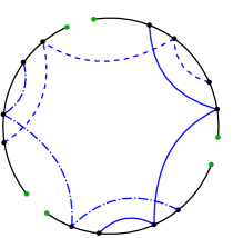
(b) Diagram $A_{4,1}^{(3,4)}$

Figure 15:

If we cut an $m$-symmetric loopless generalized chord diagram, we obtain a loopless generalized $m$-linear diagram. The converse is not true: if points $v$ and $v\mathchar 8235\relax\nobreak 1$, $2v$ and $2v\mathchar 8235\relax\nobreak 1$, $\ldots$, $m\mathchar 8705\relax\nobreak v$ and $1$ are connected by edges in a loopless generalized $m$-linear diagram, then gluing this diagram back into a chord diagram results in $m$ loops in it (Figure 15(a) and 16(a)). Denote by $A_{v,k}^{(m,d)}$ the set of generalized $m$-linear diagrams having exactly $k$ loops in each of $m$ of its sectors. The numbers $f(d\mathchar 8705\relax\nobreak n,m)$ can be expressed through the numbers $\widetilde{a}_{v,k}^{(m,d)}$ of generalized $m$-linear diagrams $A_{v,k}^{(m,d)}$ by the formula

$$f(d\mathchar 8705\relax\nobreak n,m)=\widetilde{a}_{v,0}^{(m,d)}-\sum\limits_{l\mid m}\sum\limits_{k=0}^{\widetilde{d}-2}\dfrac{l^{k}}{(\widetilde{d}-2-k)!}\mathchar 8705\relax\nobreak\widetilde{p}_{k}^{\,(\widetilde{d},l)}\mathchar 8705\relax\nobreak\widetilde{a}_{v-\widetilde{d},k}^{(m,d)},$$ (11)

where $\widetilde{d}\mathchar 12349\relax\nobreak ld/m$. To prove this formula we need to show that the number of generalized loopless $m$-linear diagrams having vertices $i\mathchar 8705\relax\nobreak v$ and $i\mathchar 8705\relax\nobreak v\mathchar 8235\relax\nobreak 1$, $i\mathchar 12349\relax\nobreak 1,2,\ldots,m$ connected by edges $e_{i}\mathchar 12349\relax\nobreak\{i\mathchar 8705\relax\nobreak v,i\mathchar 8705\relax\nobreak v\mathchar 8235\relax\nobreak 1\}$ is expressed by the formula

$$\sum\limits_{l\mid m}\sum\limits_{k\mathchar 12349\relax\nobreak 0}^{\widetilde{d}\mathchar 8704\relax\nobreak 2}\dfrac{l^{k}}{(\widetilde{d}\mathchar 8704\relax\nobreak 2\mathchar 8704\relax\nobreak k)!}\mathchar 8705\relax\nobreak\widetilde{p}_{k}^{\,(\widetilde{d},l)}\mathchar 8705\relax\nobreak\widetilde{a}_{v\mathchar 8704\relax\nobreak\widetilde{d},k}^{(m,d)}.$$

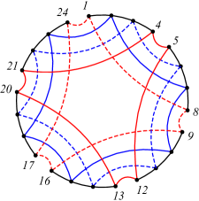
(a) Diagram $A_{4,0}^{(6,6)}$

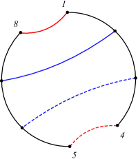
(b) Reduced diagram $A_{4,0}^{(2,2)}$

Figure 16:

In the general case, $m$ edges $e_{i}$ may belong to $l$ different subgraphs $K_{d}$, $l\mathchar 12349\relax\nobreak 1,\ldots,m$ (see Figure 16(a)). Due to the symmetry of the diagram, $l$ must divide $m$. In addition, each clique $K_{d}$ covers $m/l$ loops and hence is $m/l$ symmetric. Consequently, $m/l$ must divide $d$.

Note that it is sufficient to consider the case $l\mathchar 12349\relax\nobreak m$ where every edge $e_{i}$ belongs to its own subgraph $K_{d}$ (see Figure 15(a)). Indeed, for any diagram with $l\mathrel{\not\mathchar 12349\relax\nobreak\nobreak}m$ (see Figure 16(a)) we can select $l$ neighboring sectors ($l\mathchar 12349\relax\nobreak 2$ on Figure 16(a)) and build a reduced diagram with $l\mathchar 8705\relax\nobreak v$ points and $K_{\widetilde{d}}$ subgraphs (see Figure 16(b)), in which every edge $e_{i}$ that connects the points $i\mathchar 8705\relax\nobreak v$ and $i\mathchar 8705\relax\nobreak v\mathchar 8235\relax\nobreak 1$ belongs to its own subgraphs $K_{\widetilde{d}}$. Conversely, taking $m/l$ copies of such reduced diagrams and gluing them one after another we will obtain the diagram $A_{v,0}^{(m,d)}$. Consequently, it is sufficient to prove the formula (11) for the special case $l\mathchar 12349\relax\nobreak m$ and $\widetilde{d}\mathchar 12349\relax\nobreak d$. In other words, it is sufficient to prove that the number of generalized $m$-linear diagrams in which the points $i\mathchar 8705\relax\nobreak v$ and $i\mathchar 8705\relax\nobreak v\mathchar 8235\relax\nobreak 1$, $i\mathchar 12349\relax\nobreak 1,2,\ldots,m$ are connected by edges $e_{i}\mathchar 12349\relax\nobreak\{i\mathchar 8705\relax\nobreak v,i\mathchar 8705\relax\nobreak v\mathchar 8235\relax\nobreak 1\}$ each belonging to a separate subgraph $K_{d}$ can be calculated by the formula

$$\sum\limits_{k=0}^{\widetilde{d}-2}\dfrac{m^{k}}{(d-2-k)!}\mathchar 8705\relax\nobreak\widetilde{p}_{d-2-k}^{\,(d,m)}\mathchar 8705\relax\nobreak\widetilde{a}_{v-d,k}^{(l,d)}.$$ (12)

In order to prove (12) consider a diagram $A_{v,0}^{(m,d)}$ and delete from it all $m$ subgraphs $K_{d}$ that contain edges $e_{i}$, $i\mathchar 12349\relax\nobreak 1,\ldots,m$. The resulting diagram has $v\mathchar 8704\relax\nobreak d$ vertices and $k$ loops in each of $m$ sectors ($v\mathchar 8704\relax\nobreak d\mathchar 12349\relax\nobreak 4$, $k\mathchar 12349\relax\nobreak 1$ on Figure 15 (b)). The parameter $k$ varies from zero to $d\mathchar 8704\relax\nobreak 2$; in particular the maximal value $k\mathchar 12349\relax\nobreak d\mathchar 8704\relax\nobreak 2$ corresponds to the case where for every point being deleted appears a new loop, unless this point is an end point of a sector. The number of ways to create a generalized $m$-linear diagram with $k$ loops is equal to $a_{v\mathchar 8704\relax\nobreak d,k}^{(m,d)}$. We need to count the number of ways to form a chord diagram $A_{v,0}^{(m,d)}$ with edges $e_{i}$ connecting the vertices $i\mathchar 8705\relax\nobreak v$ and $i\mathchar 8705\relax\nobreak v\mathchar 8235\relax\nobreak 1$, $i\mathchar 12349\relax\nobreak 1,\ldots,m$ from each such diagram $A_{v\mathchar 8704\relax\nobreak d,k}^{(m,d)}$.

Note that there are no chords in a diagram $A_{v,0}^{(m,d)}$. Hence we must insert a vertex into each of $k$ loops of the diagram $A_{v\mathchar 8704\relax\nobreak d,k}^{(m,d)}$. That could be done in $m^{k}$ ways. In addition, we must insert $d\mathchar 8704\relax\nobreak k\mathchar 8704\relax\nobreak 2$ internal (that would not lie on a sector end) vertices of the cliques $K_{d}$ into each sector of the diagram. We can add these vertices one after another, and that explains the divisor $(d\mathchar 8704\relax\nobreak 2\mathchar 8704\relax\nobreak k)!$ in the denominator of the formula (12). In addition, we will assume that the points that fall into any of $k$ loops of the diagram are placed to the right of any $k$ points that were inserted into $k$ loops of the diagram $A_{v\mathchar 8704\relax\nobreak d,k}^{(m,d)}$ on the first step.

Figure 17:

Consider a sector of a diagram $A_{v\mathchar 8704\relax\nobreak d,k}^{(m,d)}$ (Figure 17). Assume that we’ve already added $j$ points into it. On Figure 17 those $v\mathchar 8704\relax\nobreak d$ points that belong to the original diagram $A_{v\mathchar 8704\relax\nobreak d,k}^{(m,d)}$ are shown in blue, $k$ points inserted on the first step are shown in yellow, and $j$ additional points are shown in red. Note that the process of adding points to the diagram $A_{v\mathchar 8704\relax\nobreak d,k}^{(m,d)}$ potentially creates some $\widetilde{k}$ additional loops ($\widetilde{k}\mathchar 12349\relax\nobreak 2$ on Figure 17). The number $q_{\widetilde{k},j\mathchar 8235\relax\nobreak 1}$ of ways to insert $j\mathchar 8235\relax\nobreak 1$ points into a sector in such a way that the number of loops $\widetilde{k}$ stays the same can be expressed through the numbers $q_{\widetilde{k}\mathchar 8704\relax\nobreak 1,j}$, $q_{\widetilde{k},j}$ and $q_{\widetilde{k}\mathchar 8235\relax\nobreak 1,j}$ by the formula

$$\begin{array}[]{c}q_{\widetilde{k},j+1}=[2j+k-(\widetilde{k}-1)]\,q_{\widetilde{k}-1,j}+(\widetilde{k}+1)(m-1)q_{\widetilde{k}+1,j}+\\[8.61108pt] +[m(v-d+j+1)-(2j-\widetilde{k}+k)-\widetilde{k}(m-1)]q_{\widetilde{k},j},\\[8.61108pt] q_{0,0}=1,\qquad\qquad q_{\widetilde{k},j}=0\,\,\text{for $\widetilde{k}\mathchar 12604\relax\nobreak 0$ or $\widetilde{k}\mathchar 12606\relax\nobreak j$}.\end{array}$$ (13)

Indeed, consider a diagram with $j$ red points and $\widetilde{k}\mathchar 8704\relax\nobreak 1$ loops. To add a new red point into it in a way that creates one new loop, we can add it either on the left or on the right of any of $j$ red points, or to the right of any yellow point. However this counts each position that falls into one of $\widetilde{k}\mathchar 8704\relax\nobreak 1$ loops twice. Consequently, the total number of positions to insert $(j\mathchar 8235\relax\nobreak 1)$-th point is equal to $2j\mathchar 8235\relax\nobreak k\mathchar 8704\relax\nobreak(\widetilde{k}\mathchar 8704\relax\nobreak 1)$.

To explain the multiplier $(\widetilde{k}\mathchar 8235\relax\nobreak 1)(m\mathchar 8704\relax\nobreak 1)$ of $q_{\widetilde{k}\mathchar 8235\relax\nobreak 1,j}$ recall that we must insert a point to destroy one of $\widetilde{k}\mathchar 8235\relax\nobreak 1$ existing loops. Let such loop belong to some subgraph $K_{d}$. We destroy this loop in case the new point belongs to one of $m\mathchar 8704\relax\nobreak 1$ remaining complete subgraphs $K_{d}$. Consequently, there are $(\widetilde{k}\mathchar 8235\relax\nobreak 1)(m\mathchar 8704\relax\nobreak 1)$ ways to insert this point.

Finally consider a diagram with $j$ red points and $\widetilde{k}$ loops. This diagram has $v\mathchar 8704\relax\nobreak d\mathchar 8235\relax\nobreak j\mathchar 8235\relax\nobreak 1$ positions for inserting a new red point. More than that, this red point may belong to any of $m$ subgraphs $K_{d}$ that will be added. This fact explains the multiplier $m(v\mathchar 8704\relax\nobreak d\mathchar 8235\relax\nobreak j\mathchar 8235\relax\nobreak 1)$ in formula (13). However we should exclude those positions that lead to a new loop or to a destruction of an existing loop. A new loop can be added in $2j\mathchar 8704\relax\nobreak\widetilde{k}\mathchar 8235\relax\nobreak k$ ways, and one of the existing loops can be destroyed in $(m\mathchar 8704\relax\nobreak 1)\widetilde{k}$ ways.

Using the recurrence relation (13) we can calculate the numbers $q_{\widetilde{k},j}$ up to $j\mathchar 12349\relax\nobreak d\mathchar 8704\relax\nobreak 2\mathchar 8704\relax\nobreak k$. We will need the numbers $q_{0,j}$ which describe the ways to add $j$ points so that there are no loops after the addition.

The final step of building a loopless $m$-linear diagram is the addition of two end vertices to each sector. If these vertices do not belong to the same subgraph $K_{d}$ as their neighbors, there are no loops added and the number of ways to do that coincides with $q_{0,\widetilde{v}}$, $\widetilde{v}:\mathchar 12349\relax\nobreak d\mathchar 8704\relax\nobreak 2\mathchar 8704\relax\nobreak k$. However there exists a possibility that one or two of the end vertices creates a new loop. Hence the number $\widetilde{p}_{v}$ of loopless diagrams with added end vertices can be expressed through the numbers $q_{0,j}$ using inclusion-exclusion principle:

$$\widetilde{p}_{\widetilde{v}}^{\,(d,m)}\mathchar 12349\relax\nobreak\sum\limits_{i\mathchar 12349\relax\nobreak 0}^{\widetilde{v}}\sum\limits_{j\mathchar 12349\relax\nobreak 0}^{\widetilde{v}\mathchar 8704\relax\nobreak i}(\mathchar 8704\relax\nobreak 1)^{i\mathchar 8235\relax\nobreak j}\mathchar 8705\relax\nobreak\frac{\widetilde{v}!}{(\widetilde{v}\mathchar 8704\relax\nobreak i\mathchar 8704\relax\nobreak j)!}\mathchar 8705\relax\nobreak q_{0,\widetilde{v}\mathchar 8704\relax\nobreak i\mathchar 8704\relax\nobreak j}.$$

In this formula the summation runs over the number $i$ of leftmost points that belong to the same clique as the point being added, and over an analogous number $j$ of rightmost points.

To use the formula (11) it remains to obtain some recurrence relations for the numbers $a_{v,k}^{(m,d)}$. In fact, these numbers can be counted by the following formulas:

$$a_{v,k}^{(m,d)}=\sum\limits_{l\mid m}\sum\limits_{t=k-\widetilde{d}+1}^{k+\widetilde{d}-1}c_{k,t}\mathchar 8705\relax\nobreak a_{v-\widetilde{d},t}^{(l,\widetilde{d})},$$ (14)

where

$$c_{k,t}=\sum\limits_{i=0}^{\widetilde{d}-1}{{\widetilde{d}-1}\choose{i}}\mathchar 8705\relax\nobreak{{t}\choose{t+i-k}}\mathchar 8705\relax\nobreak\dfrac{l^{t+i-k}}{(\widetilde{d}-2i-t+k-1)!}\mathchar 8705\relax\nobreak\widehat{p}_{d-2i-t+k-1}.$$ (15)

Note that to prove the formulas (14)–(15) it is also sufficient to consider the case $l\mathchar 12349\relax\nobreak m$, $\widetilde{d}\mathchar 12349\relax\nobreak d$: all the other cases can be reduced to it analogously as for (11).

In particular, to prove (14) remove $m$ cliques that contain the leftmost points of each of $m$ sectors. This yields a diagram $A_{v\mathchar 8704\relax\nobreak d,t}^{(m,d)}$ with $v\mathchar 8704\relax\nobreak d$ vertices and $t$ loops in each sector. The number of ways to obtain such diagram is $a_{v\mathchar 8704\relax\nobreak d,t}^{(m,d)}$. It remains to find the numbers $c_{k,t}$ of ways to add $m$ cliques back to an arbitrary diagram $A_{v\mathchar 8704\relax\nobreak d,t}^{(m,d)}$.

Denote by $i$ the number of loops belonging to a clique $K_{d}$. Contracting such loops we obtain a clique with $d\mathchar 8704\relax\nobreak i$ vertices. The loops can be restored in $\left(\!\!{{d\mathchar 8704\relax\nobreak i}\choose{i}}\!\!\right)\mathchar 12349\relax\nobreak{{d\mathchar 8704\relax\nobreak 1}\choose{i}}$ ways. Then, similarly to the derivation of (3), we have to obtain $k$ loops in each sector, hence out of the existing $t$ loops we must destroy $t\mathchar 8235\relax\nobreak i\mathchar 8704\relax\nobreak k$. Since each loop could be destroyed by any of $m$ cliques, we should multiply the binomial coefficient ${{t}\choose{t\mathchar 8235\relax\nobreak i\mathchar 8704\relax\nobreak k}}$ by $m^{t\mathchar 8235\relax\nobreak i\mathchar 8704\relax\nobreak k}$. It remains to add $v:\mathchar 12349\relax\nobreak d\mathchar 8704\relax\nobreak 2i\mathchar 8704\relax\nobreak t\mathchar 8235\relax\nobreak k\mathchar 8704\relax\nobreak 1$ vertices to each sector (or to each clique). These vertices can be added one by one, and that explains the divisor $(d\mathchar 8704\relax\nobreak 2i\mathchar 8704\relax\nobreak t\mathchar 8235\relax\nobreak k\mathchar 8704\relax\nobreak 1)$ in the formula (15). Finally, the numbers $\widehat{p}$ express the number of ways to add the vertices in such a way that the resulting diagram has no loops. The numbers $\widehat{p}$ are expressed through $q_{0,j}$ by the formula

$$\widehat{p}_{\widehat{v}}\mathchar 12349\relax\nobreak\sum\limits_{i\mathchar 12349\relax\nobreak 0}^{\widehat{v}}(\mathchar 8704\relax\nobreak 1)^{i}\mathchar 8705\relax\nobreak\frac{\widehat{v}!}{(\widehat{v}\mathchar 8704\relax\nobreak i)!}\mathchar 8705\relax\nobreak q_{0,\widehat{v}\mathchar 8704\relax\nobreak i}.$$

5 Enumeration of Hamiltionian cycles in $K_{d,d,\ldots,d}$ up to reflections and rotations

In this section we enumerate non-isomorphic chord diagrams under the action of the dihedral group $D_{d\mathchar 8705\relax\nobreak n}$. The Burnside lemma could be rewritten for this case as

$$\widetilde{b}_{n}=\dfrac{1}{2dn}\sum\limits_{m\,|\,dn}\varphi(m)\,f(dn,m)+\dfrac{h^{(0)}(n)+2h^{(1)}(n)+h^{(2)}(n)}{2},$$ (16)

where $h^{(i)}(n)$ denotes the number of chord diagrams symmetric under reflection about the axis passing through $i$ points of the diagram and consisting of $n$ subgraphs $K_{d}$ (see Figure 18).

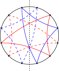
(a) Diagram $H^{(0)}(4)$

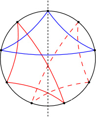
(b) Diagram $H^{(1)}(3)$

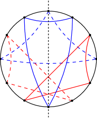
(c) Diagram $H^{(2)}(4)$

Figure 18:

First consider the case of the axis of symmetry not passing through any vertices (Figure 18 (a)). The number $dn$ of points must be even in this case. We can transform any such diagram into some generalized $2$-linear diagram having $dn/2$ points by cutting the circle between the points $1$ and $dn$, between the points $dn/2$ and $dn/2\mathchar 8235\relax\nobreak 1$ (Figure 19 (a)), and then reflecting one half of the diagram along the horizontal axis (Figure 19 (b)). However, the mapping described by this transformation may be not bijective: if a $2$-linear diagram has edges $e_{1}$ and $e_{2}$ connecting the vertices $1$ and $dn/2\mathchar 8235\relax\nobreak 1$, as well as $dn$ and $dn/2$, the reverse mapping would create two loops in the new diagram.

(a) Diagram $H^{(0)}(4)$

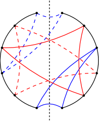
(b) Diagram $A_{6,0}^{(2,3)}$

Figure 19:

Note that for an odd $d$ the described mapping is actually bijective. Indeed, any edge $e_{i}$ must belong to some subgraph $K_{d}$ which must be transformed into itself by a reflection along the vertical axis, and that is impossible for odd $d$. So for odd $d$ we have

$$h^{(0)}(n)\mathchar 12349\relax\nobreak a_{dn/2,0}^{(2,d)}.$$

For an even $d$ the formula is more complex: a generalized $2$-linear diagram may have both edges $e_{i}$ or any of them separately. Then for $h^{(0)}(n)$ we have the following formula:

$$h^{(0)}(n)\mathchar 12349\relax\nobreak a_{dn/2,0}^{(2,d)}\mathchar 8704\relax\nobreak 2\sum\limits_{k\mathchar 12349\relax\nobreak 0}^{d/2\mathchar 8704\relax\nobreak 1}\alpha^{(1)}_{k}\mathchar 8705\relax\nobreak a_{d(n\mathchar 8704\relax\nobreak 1)/2,k}^{(2,d)}\mathchar 8235\relax\nobreak\sum\limits_{k\mathchar 12349\relax\nobreak 0}^{d\mathchar 8704\relax\nobreak 2}\alpha^{(2)}_{k}\mathchar 8705\relax\nobreak a_{d(n\mathchar 8704\relax\nobreak 2)/2,k}^{(2,d)}\mathchar 8704\relax\nobreak\sum\limits_{k\mathchar 12349\relax\nobreak 0}^{d/2\mathchar 8704\relax\nobreak 2}\alpha^{(3)}_{k}\mathchar 8705\relax\nobreak a_{d(n\mathchar 8704\relax\nobreak 2)/2,k}^{(2,d)},$$

$$\alpha^{(1)}_{k}:\mathchar 12349\relax\nobreak{{(n\mathchar 8704\relax\nobreak 1)d/2\mathchar 8704\relax\nobreak 1\mathchar 8704\relax\nobreak k}\choose{d/2\mathchar 8704\relax\nobreak 1\mathchar 8704\relax\nobreak k}},\qquad\qquad\alpha^{(3)}_{k}:\mathchar 12349\relax\nobreak{{(n\mathchar 8704\relax\nobreak 1)d/2\mathchar 8704\relax\nobreak 1\mathchar 8704\relax\nobreak k}\choose{d/2\mathchar 8704\relax\nobreak 2\mathchar 8704\relax\nobreak k}},$$

$$\alpha^{(2)}_{k}:\mathchar 12349\relax\nobreak\sum\limits_{j\mathchar 12349\relax\nobreak 0}^{d/2\mathchar 8704\relax\nobreak 1}\sum\limits_{s\mathchar 12349\relax\nobreak 0}^{\min(k,d/2\mathchar 8704\relax\nobreak 1\mathchar 8704\relax\nobreak j)}{{d/2\mathchar 8704\relax\nobreak 1}\choose{j}}\mathchar 8705\relax\nobreak{{k}\choose{s}}\mathchar 8705\relax\nobreak{{d/2(n\mathchar 8704\relax\nobreak 2)\mathchar 8704\relax\nobreak k}\choose{d/2\mathchar 8704\relax\nobreak 1\mathchar 8704\relax\nobreak j\mathchar 8704\relax\nobreak s}}\mathchar 8705\relax\nobreak{{d/2(n\mathchar 8704\relax\nobreak 1)\mathchar 8704\relax\nobreak 1\mathchar 8704\relax\nobreak(k\mathchar 8235\relax\nobreak j\mathchar 8704\relax\nobreak s)}\choose{d/2\mathchar 8704\relax\nobreak 1\mathchar 8704\relax\nobreak(k\mathchar 8235\relax\nobreak j\mathchar 8704\relax\nobreak s)}}.$$

The coefficients $\alpha^{(1)}_{k}$ describe the diagrams which have an edge $e$ connecting either the pair $1$ and $dn/2\mathchar 8235\relax\nobreak 1$ or the pair $dn$ and $dn/2$; the coefficients $\alpha^{(2)}_{k}$ describe the diagrams that have both of these pairs of vertices connected by edges $e_{i}$, $i\mathchar 12349\relax\nobreak 1,2$, belonging to two different subgraphs $K_{d}$; the coefficients $\alpha^{(3)}_{k}$ describe an analogous case when both $e_{i}$ belong to the same subgraph $K_{d}$.

To find the coefficients $\alpha^{(1)}_{k}$ delete the subgraph $K_{d}$ containing the edge $e$ from a generalized $2$-linear diagram $A_{nd/2,0}^{(2,d)}$. This yields a generalized $2$-linear diagram $A_{d/2(n\mathchar 8704\relax\nobreak 1),k}^{(2,d)}$ with $k$ loops in each sector, $k\mathchar 12349\relax\nobreak 0,\ldots,d/2\mathchar 8704\relax\nobreak 2$. There are $\alpha^{(1)}_{k}$ ways to add a subgraph $K_{d}$ back to this diagram. Indeed, exactly $k$ out of $d/2\mathchar 8704\relax\nobreak 1$ points of the subgraph $K_{d}$ must be placed into $k$ loops of each of two sectors, one point must be placed on the end of each sector, and then the remaining $d/2\mathchar 8704\relax\nobreak 1\mathchar 8704\relax\nobreak k$ points of the subgraph $K_{d}$ can be distributed among $(n\mathchar 8704\relax\nobreak 1)d/2\mathchar 8704\relax\nobreak 1$ positions in ${{(n\mathchar 8704\relax\nobreak 1)d/2\mathchar 8704\relax\nobreak 1\mathchar 8704\relax\nobreak k}\choose{d/2\mathchar 8704\relax\nobreak 1\mathchar 8704\relax\nobreak k}}$ ways.

Consider the case of a linear diagram $A_{nd/2,0}^{(2,d)}$ having both pairs of edges connected by $e_{i}$. These edges could belong either to the same subgraph $K_{d}$ or to two different subgraphs. It would be easier to deal with the former subcase first. Removing the subgraph $K_{d}$ yields a diagram $A_{d/2(n\mathchar 8704\relax\nobreak 1),k}^{(2,d)}$, for which $d/2\mathchar 8704\relax\nobreak 2\mathchar 8704\relax\nobreak k$ points of the subgraph $K_{d}$ must be distributed among $d/2\mathchar 8704\relax\nobreak 2\mathchar 8704\relax\nobreak k$ positions. This could be done in $\alpha^{(3)}_{k}$ ways. In the latter subcase removing both subgraphs $K_{d}$ yields a $2$-linear diagram $A_{d/2(n\mathchar 8704\relax\nobreak 2),k}^{(2,d)}$ with $k$ loops $k\mathchar 12349\relax\nobreak 0,\ldots,d\mathchar 8704\relax\nobreak 2$. Enumerating the ways to add these two subgraphs back results in almost the same considerations as those that were performed to find the coefficients $p_{n,R,m}$.

Namely, first we add the subgraph $K_{d}$ that contains the edge $e_{1}$ into a diagram $A_{d/2(n\mathchar 8704\relax\nobreak 2),k}^{(2,d)}$. Denote by $s$ the number of loops of the diagram that are destroyed by the vertices of $K_{d}$. Denote by $j$ the number of loops belonging to $K_{d}$ which are created in each sector. Contracting these loops we obtain a reduced subgraph with $d\mathchar 8704\relax\nobreak 2j$ vertices. One vertex of this subgraph must be placed onto the first position of a sector. Then there are ${{k}\choose{s}}$ ways to place the vertices into $s$ loops and ${{(n\mathchar 8704\relax\nobreak 2)d/2\mathchar 8704\relax\nobreak k}\choose{d/2\mathchar 8704\relax\nobreak 1\mathchar 8704\relax\nobreak j\mathchar 8704\relax\nobreak s}}$ ways to distribute the remaining vertices over positions not covered by loops. Finally there are ${{d/2\mathchar 8704\relax\nobreak 1}\choose{j}}$ ways to split $j$ vertices and transform them into the loops of $K_{d}$. The last binomial coefficient in $\alpha^{(2)}_{k}$ describes the number of ways to add the second subgraph $K_{d}$ so that the obtained diagram has no loops.

The numbers $h^{(1)}_{n}$ describing symmetric diagrams with a single vertex lying on the axis of symmetry may be different from $0$ only for odd $n$ and $d$. Removing the subgraph $K_{d}$ which contains the vertex lying on the axis of symmetry and flipping one half of the diagram yields a generalized $2$-linear diagram $A_{d(n\mathchar 8704\relax\nobreak 1)/2,k}^{(2,d)}$ containing $k$ loops in each sector. Since the reverse transformation could be done in ${{(n\mathchar 8704\relax\nobreak 1)d/2\mathchar 8704\relax\nobreak 1\mathchar 8704\relax\nobreak k}\choose{(d\mathchar 8704\relax\nobreak 1)/2\mathchar 8704\relax\nobreak k}}$ ways, the numbers $h^{(1)}(n)$ are equal to

$$h^{(1)}(n)\mathchar 12349\relax\nobreak\sum\limits_{k\mathchar 12349\relax\nobreak 0}^{(d\mathchar 8704\relax\nobreak 1)/2}{{(n\mathchar 8704\relax\nobreak 1)d/2\mathchar 8704\relax\nobreak 1\mathchar 8704\relax\nobreak k}\choose{(d\mathchar 8704\relax\nobreak 1)/2\mathchar 8704\relax\nobreak k}}\mathchar 8705\relax\nobreak a_{d(n\mathchar 8704\relax\nobreak 1)/2,k}^{(2,d)}.$$

It remains to consider the case of the axis of symmetry crossing two vertices. For an even $d$ these vertices must belong to the same clique $K_{d}$. Considerations analogous to those performed above for counting $h^{(1)}(n)$ yield that

$$h^{(2)}(n)\mathchar 12349\relax\nobreak\sum\limits_{k\mathchar 12349\relax\nobreak 0}^{d/2\mathchar 8704\relax\nobreak 1}\alpha^{(1)}_{k}\mathchar 8705\relax\nobreak a_{d(n\mathchar 8704\relax\nobreak 1)/2,k}^{(2,d)},\qquad\qquad\text{$d$ is even}.$$

For an odd $d$ the numbers $h^{(2)}(n)$ may be different from $0$ only if $n$ is even. They can be calculated by the formula

$$h^{(2)}(n)\mathchar 12349\relax\nobreak\sum\limits_{k\mathchar 12349\relax\nobreak 0}^{d\mathchar 8704\relax\nobreak 1}\sum\limits_{j\mathchar 12349\relax\nobreak 0}^{(d\mathchar 8704\relax\nobreak 1)/2}\sum\limits_{s\mathchar 12349\relax\nobreak 0}^{\min(k,(d\mathchar 8704\relax\nobreak 1)/2\mathchar 8704\relax\nobreak j)}{{(d\mathchar 8704\relax\nobreak 1)/2}\choose{j}}{{k}\choose{s}}{{d/2(n\mathchar 8704\relax\nobreak 2)\mathchar 8704\relax\nobreak k}\choose{(d\mathchar 8704\relax\nobreak 1)/2\mathchar 8704\relax\nobreak j\mathchar 8704\relax\nobreak s}}\mathchar 8706\relax\nobreak$$

$$\mathchar 8706\relax\nobreak{{d/2(n\mathchar 8704\relax\nobreak 1)\mathchar 8704\relax\nobreak 1\mathchar 8704\relax\nobreak(k\mathchar 8235\relax\nobreak j\mathchar 8704\relax\nobreak s)}\choose{(d\mathchar 8704\relax\nobreak 1)/2\mathchar 8704\relax\nobreak(k\mathchar 8235\relax\nobreak j\mathchar 8704\relax\nobreak s)}}\mathchar 8705\relax\nobreak a_{d(n\mathchar 8704\relax\nobreak 2)/2,k}^{(2,d)}.$$

Conclusion

In this paper labelled and unlabelled generalized loopless chord and linear diagrams were enumerated. Labelled chord diagrams can be thought of as directed Hamiltonian cycles with a distinguished starting point in unlabelled graphs $K_{d,d,\ldots,d}$. Considering chord diagrams up to rotations removes the starting point but keeps the direction chosen. Finally, chord diagrams considered up to rotations and reflections is nothing but undirected unlabelled Hamiltonian cycles in unlabelled graphs $K_{d,d,\ldots,d}$. The final numbers for various classes of linear and chord diagrams as well as Hamiltonian cycles considered above can be found in Tables 1–5.

$n$	0Linear0	0Chord labelled0	0Up to rotations0	0Up to all symmetries0
1	0	0	0	0
2	1	1	1	1
3	5	4	2	2
4	36	31	7	7
5	329	293	36	29
6	3655	3326	300	196
7	47844	44189	3218	1788
8	721315	673471	42335	21994
9	12310199	11588884	644808	326115
10	234615096	222304897	11119515	5578431
11	4939227215	4704612119	213865382	107026037
12	113836841041	108897613826	4537496680	2269254616
13	2850860253240	2737023412199	105270612952	52638064494
14	77087063678521	74236203425281	2651295555949	1325663757897
15	2238375706930349	2161288643251828	72042968876506	36021577975918
16	69466733978519340	67228358271588991	2100886276796969	1050443713185782
17	2294640596998068569	2225173863019549229	65446290562491916	32723148860301935
18	80381887628910919255	78087247031912850686	2169090198219290966	1084545122297249077
19	2976424482866702081004	2896042595237791161749	76211647261082309466	38105823782987999742
20	116160936719430292078411	113184512236563589997407	2829612806029873399561	1414806404051118314077

Table 1: Loopless diagrams by number of $K_{2}$

$n$	0Linear0	0Chord labelled0	0Up to rotations0	0Up to all symmetries0
1	0	0	0	0
2	1	1	1	1
3	29	22	4	4
4	1721	1415	126	83
5	163386	140343	9367	4848
6	22831355	20167651	1120780	562713
7	4420321081	3980871156	189565588	94810999
8	1133879136649	1035707510307	43154533233	21577786374
9	372419001449076	343866839138005	12735808866899	6367912802891
10	152466248712342181	141979144588872613	4732638168795171	2366319275431001
11	76134462292157828285	71386289535825383386	2163220895025390670	1081610451348718567
12	45552714996556390334921	42954342000612934599071	1193176166690983987122	596588083450068950934
13	32173493282909179882613934	30482693813120122213093587	781607533669746761791541	390803766837390136477505

Table 2: Loopless diagrams by number of $K_{3}$

$n$	0Linear0	0Chord labelled0	0Up to rotations0	0Up to all symmetries0
1	0	0	0	0
2	1	1	1	1
3	182	134	15	13
4	94376	75843	4790	2576
5	98371884	83002866	4151415	2081393
6	182502973885	158861646466	6619291247	3309962320
7	551248360550999	490294453324924	17510518983528	8755277273334
8	2536823683737613858	2292204611710892971	71631394311300461	35815698613833466
9	16904301142107043464659	15459367618357013402267	429426878302882412435	214713439275724149414
10	156690501089429126239232946	144663877588996810362218074	3616596939726424941979785	1808298469877117320495867

Table 3: Loopless diagrams by number of $K_{4}$

$n$	0Linear0	0Chord labelled0	0Up to rotations0	0Up to all symmetries0
1	0	0	0	0
2	1	1	1	1
3	1198	866	60	42
4	5609649	4446741	222477	112418
5	66218360625	55279816356	2211192688	1105696796
6	1681287695542855	1450728060971387	48357603758012	24178822553773
7	81644850343968535401	72078730629785795963	2059392303708166507	1029696155560021174
8	6945222145021508480249929	6235048155225093080061949	155876203880714141444480	77938101941693076258854

Table 4: Loopless diagrams by number of $K_{5}$

$n$	0Linear0	0Chord labelled0	0Up to rotations0	0Up to all symmetries0
1	0	0	0	0
2	1	1	1	1
3	8142	5812	335	203
4	351574834	276154969	11508322	5765385
5	47940557125969	39738077935264	1324603148183	662305416760
6	16985819072511102549	14571371516350429940	404760320241653655	202380163158922023
7	13519747358522016160671387	11876790400066163254723167	282780723811372935744420	141390361908351519807928

Table 5: Loopless diagrams by number of $K_{6}$

References

[1]
Carsten Thomassen.
On the number of hamiltonian cycles in bipartite graphs.
Combinatorics, Probability and Computing, 5:437–442, 1996.
[2]
Noga Alon.
The maximum number of hamiltonian paths in tournaments.
Combinatorica, 10(4):319–324, 1990.
[3]
Endre Szemeredi Gabor N. Sarkozya, Stanley M. Selkowa.
On the number ofhamiltonian cycles in dirac graphs.
Discrete Mathematics, 265(237-250), 2003.
[4]
Allen J. Schwenk.
Enumeration of hamiltonian cycles in certain generalized petersen
graphs.
J. Combin. Theory Ser. B, 47:53–59, 1989.
[5]
E. Dixon and S. Goodman.
On the number of hamiltonian circuits in the n-cube.
Proceedings of the American Mathematical Society, 50:500–504,
1975.
[6]
David Singmaster.
Hamiltonian circuits on the n-dimensional octahedron.
Journal of Combinatorial Theory, Series B, 19(1):1–4, 1975.
[7]
M. Hazewinkel and V.V. Kalashnikov.
Counting Interlacing Pairs on the Circle.
Department of Analysis, Algebra and Geometry: Report AM. Stichting
Mathematisch Centrum, 1995.
[8]
A.V.Omelchenko E.S.Krasko.
Enumeration of chord diagrams without loops and parallel chords.
The Electronic Journal of Combinatorics, 2017.
[9]
Richard J. Mathar.
A class of multinomial permutations avoiding object clusters.
viXra:1511.0015.