A solvable model of Vlasov-kinetic plasma turbulence in Fourier-Hermite phase space

Abstract

A class of simple kinetic systems is considered, described by the 1D Vlasov–Landau equation with Poisson or Boltzmann electrostatic response and an energy source. Assuming a stochastic electric field, a solvable model is constructed for the phase-space turbulence of the particle distribution. The model is a kinetic analog of the Kraichnan–Batchelor model of chaotic advection. The solution of the model is found in Fourier–Hermite space and shows that the free-energy flux from low to high Hermite moments is suppressed, with phase mixing cancelled on average by anti-phase-mixing (stochastic plasma echo). This implies that Landau damping is an ineffective route to dissipation (i.e., to thermalisation of electric energy via velocity space). The full Fourier–Hermite spectrum is derived. Its asymptotics are $m^{-3/2}$ at low wave numbers and high Hermite moments ($m$) and $m^{-1/2}k^{-2}$ at low Hermite moments and high wave numbers ($k$). These conclusions hold at wave numbers below a certain cut off (analog of Kolmogorov scale), which increases with the amplitude of the stochastic electric field and scales as inverse square of the collision rate. The energy distribution and flows in phase space are a simple and, therefore, useful example of competition between phase mixing and nonlinear dynamics in kinetic turbulence, reminiscent of more realistic but more complicated multi-dimensional systems that have not so far been amenable to complete analytical solution.

1 Introduction

One of the most distinctive properties of a weakly collisional plasma as a physical system is the intricate phase-space dynamics associated with the interaction between electromagnetic fields and charged particles. The signature plasma-physics phenomenon of Landau (1946) damping consists essentially in the removal of free energy from an electromagnetic perturbation and its transfer “into phase space”, i.e., into fine-scale structure of the perturbed distribution function in velocity space (“phase mixing”). It has long been realised that nonlinear effects can lead to Landau damping shutting down, both for broad-spectrum fields and individual monochromatic waves (Vedenov et al., 1962; O’Neil, 1965; Mazitov, 1965; Manheimer & Dupree, 1968; Weiland, 1992), or even to apparently damped perturbations coming back from phase space, a phenomenon called “plasma echo” (Gould et al., 1967; Malmberg et al., 1968). Fast-forwarding over several decades of plasma-turbulence theory (see Krommes 2015 and Laval et al. 2016 for review and references), the notion of “phase-space turbulence”, pioneered by Dupree (1972), has, in the recent years, again become a popular object of study, treated either, Dupree-style, in terms of formation of phase-spaces structures and their effect on the transport properties of the plasma (Kosuga & Diamond, 2011; Kosuga et al., 2014, 2017; Lesur et al., 2014a, b) or in terms of a kinetic cascade carrying free energy to collisional scales in velocity space (Watanabe & Sugama, 2004; Schekochihin et al., 2008, 2009; Tatsuno et al., 2009; Plunk et al., 2010; Plunk & Tatsuno, 2011; Bañón Navarro et al., 2011; Teaca et al., 2012, 2016; Hatch et al., 2014; Kanekar, 2015; Schekochihin et al., 2016; Parker et al., 2016; Servidio et al., 2017).

Within the latter strand, a direct precursor to the present study is the paper by Schekochihin et al. (2016), who proposed, using electrostatic drift-kinetic turbulence as a prototypical example of kinetic turbulence, that a key effect of nonlinearity on phase-space dynamics would be an effective suppression of Landau damping—meaning that the free-energy flux from small to large scales in velocity space associated with stochastic echos (“anti-phase-mixing”, or “phase unmixing”) largely cancels the phase-mixing flux (“Landau damping”) from large to small scales. A signature of this effect is a Hermite spectrum of free energy that is steeper for the nonlinear, turbulent perturbations than for the linear, Landau-damped ones (seen in numerical simulations of Watanabe & Sugama 2004, Hatch et al. 2014 and Parker et al. 2016). As a result, the limit of vanishing collisionality ceases to be a singular limit at long wavelengths (as it is in the linear regime; see, e.g., Kanekar et al. 2015) and most of the entropy production occurs below the Larmor scale (i.e., outside the drift-kinetic approximation).

While some theoretical predictions of Schekochihin et al. (2016) appear to have found a degree of numerical backing (Parker et al., 2016), their theory of stochastic echo was a qualitative one, relying on plausible scaling arguments, rather like the theory of hydrodynamic turbulence mostly does to this day (Davidson, 2004). In addition to such arguments, understanding of fluid turbulence has benefited greatly from the development of simplified solvable models, the most famous of which is the “passive-scalar” model describing the behaviour of a scalar field chaotically advected by an externally determined random flow (Kraichnan, 1968, 1974, 1994; Falkovich et al., 2001). Under certain assumptions about the nature of this flow, it is possible to solve for the passive-scalar statistics analytically, leading to a number of interesting and nontrivial predictions, some of which appear to carry over qualitatively or even quantitatively to more realistic turbulent systems and all of which have proved stimulating to turbulence theorists. In view of this experience, seeking a maximally simplified but analytically solvable model appears to be worthwhile.

In this paper, we propose such a solvable model, based on the much-studied 1D Vlasov–Poisson system. The phase space for this system is two-dimensional (one spatial and one velocity coordinate). The particle distribution function in a turbulent state can be described in terms of its Fourier–Hermite spectrum. We show that, given a stochastic electric field, the only physically sensible solution features zero net free-energy flux from low (“fluid”) to high (“kinetic”) Hermite moments, meaning that the Landau damping is suppressed and the low moments are energetically insulated from the rest of the phase space. The underlying mechanism of this suppression is the stochastic-echo effect. The resulting Hermite spectrum is, asymptotically, $m^{-3/2}$ at large Hermite orders $m$ (compared to $m^{-1/2}$ for linear Landau damping; see Zocco & Schekochihin 2011 and Kanekar et al. 2015) and so the limit of small collisionality is nonsingular (collisional dissipation tends to zero if the collision rate does). The corresponding Fourier spectrum of the low-$m$ Hermite moments is $m^{-1/2}k^{-2}$. Surveyed over the entire phase space, the phase-mixing (Landau-damped) and anti-phase-mixing (echoing) components of the distribution function have an interesting and not entirely trivial self-similar structure, which can nevertheless be fully extracted analytically and bears some resemblance to what is seen in various numerical simulations. A finite collision rate imposes a finite wave-number cutoff on this solution, which is the analog of the Kolmogorov scale for the Vlasov-kinetic turbulence.

The rest of the paper is organised as follows. In section 2, we describe a family of plasma systems that can be reasonably modelled by the equations studied in this paper (electron Langmuir turbulence, ion-acoustic turbulence, Zakharov turbulence). In section 3, we recast these equations in Fourier–Hermite space and introduce the formalism within which the phase mixing anti-phase-mixing can be studied explicitly (this formalism is similar to one developed by Schekochihin et al. 2016, but with minor adjustments). In section 4, we make the approximations required to render the problem solvable and derive an equation for the Fourier–Hermite spectrum of the distribution function. In section 5, we solve this equation, obtaining the results promised above (a qualitative summary of this solution and an assessment of the effect of finite collisionality on it are given in section 5.4; a quicker, but perhaps less mathematically complete route to it than one pursued in the main text is described in appendix B). Finally, results are summarised and limitations, implications, applications and future directions discussed in section 6.

2 Models: Vlasov–Poisson system and its cousins

The standard Vlasov–Poisson system describes a plasma in the absence of magnetic field. For each species ($s=e$ electrons or $s=i$ ions), the distribution function obeys the Vlasov–Landau equation

$$\frac{\partial f_{s}}{\partial t}+\boldsymbol{v}\cdot\boldsymbol{\nabla}f_{s}-\frac{q_{s}}{m_{s}}(\boldsymbol{\nabla}\phi)\cdot\frac{\partial f_{s}}{\partial\boldsymbol{v}}=\left(\frac{\partial f_{s}}{\partial t}\right)_{\mathrm{c}},$$ (1)

where $q_{s}$ and $m_{s}$ are the charge and mass of the particles, the term in the right-hand side is the collision operator, and $\phi$ is the electrostatic potential, satisfying Poisson’s equation

$$-\nabla^{2}\phi=4\pi\sum_{s}q_{s}\int\mathrm{d}^{3}\boldsymbol{v}\,\delta\!f_{s}.$$ (2)

We are formally splitting the distribution function into mean and perturbed parts,

$$f_{s}=f_{0s}(\boldsymbol{v})+\delta\!f_{s}(t,\boldsymbol{r},\boldsymbol{v}),$$ (3)

where $f_{0s}$ is spatially homogeneous and we assume that there is no mean electric field. Only $\delta\!f_{s}$ enters the Poisson equation (2) because the plasma is neutral on average. We do not require that $\delta\!f_{s}\ll f_{0s}$ everywhere, although we do assume that any temporal evolution of the mean distribution is slow compared to that of the perturbation. We take the mean distribution to be Maxwellian,

$$f_{0s}=\frac{n_{0s}}{(\pi v_{{\rm th}s}^{2})^{3/2}}e^{-|\boldsymbol{v}|^{2}/v_{{\rm th}s}^{2}},$$ (4)

where $v_{{\rm th}s}=\sqrt{2T_{s}/m_{s}}$ is the thermal speed of the particles of species $s$ and $n_{0s}$ and $T_{s}$ are their number density and temperature, respectively.

Several simplified models can be constructed, leading to mathematically similar sets of equations.

2.1 Electron Vlasov–Poisson plasma

Assuming cold ions, or, equivalently, restricting our consideration to perturbations with frequencies of the order of the electron plasma frequency,

$$\omega\sim\omega_{\mathrm{p}e}=\sqrt{\frac{4\pi e^{2}n_{0e}}{m_{e}}},$$ (5)

where $-e\equiv q_{e}$, we may set $\delta\!f_{i}=0$. Further restricting our consideration to a single spatial dimension, $x$, we have $\delta\!f_{e}=\delta\!f_{e}(x,\boldsymbol{v})$. We may now introduce the following reduced, non-dimensionalised fields and variables:

$$g(x,v)=\frac{v_{{\rm th}e}}{n_{0e}}\int\mathrm{d}v_{y}\mathrm{d}v_{z}\delta\!f_{e},\quad F_{\mathrm{M}}(v)=\frac{1}{\sqrt{\pi}}\,e^{-v^{2}},\quad v=\frac{v_{x}}{v_{{\rm th}e}},\quad\varphi=-\frac{e\phi}{T_{e}}.$$ (6)

We may also non-dimensionalise $t\omega_{\mathrm{p}e}\to t$ and $x/\sqrt{2}\,\lambda_{\mathrm{D}e}\to x$, where $\lambda_{\mathrm{D}e}=v_{{\rm th}e}/\sqrt{2}\,\omega_{\mathrm{p}e}$ is the electron Debye length. In this notation, the Vlasov–Poisson system becomes

$$\frac{\partial g}{\partial t}+v\frac{\partial g}{\partial x}+vF_{\mathrm{M}}\frac{\partial\varphi}{\partial x}-\frac{1}{2}\frac{\partial\varphi}{\partial x}\frac{\partial g}{\partial v}=C[g],$$ (7)

$$\varphi=\alpha\int\mathrm{d}v\,g+\chi,$$ (8)

where $-\alpha$ is twice the inverse Laplacian operator, $\alpha_{k}=2/k^{2}$ in Fourier space. We have added an “external” potential $\chi$ to represent energy injection in an analytically convenient fashion (it will also acquire concrete physical meaning in sections 2.3 and 2.4). Finally, we make a further simplification by using the Lenard & Bernstein (1958) collision operator

$$C[g]=\nu\frac{\partial}{\partial v}\left(\frac{1}{2}\frac{\partial}{\partial v}+v\right)g,$$ (9)

with the proviso that it must be adjusted to conserve momentum and energy. This will not be a problem as the collision frequency $\nu$ will always be assumed small and so will only matter for the part of $g$ that varies quickly with $v$.

Besides being interesting in itself, the 1D Vlasov–Poisson system (7–8) is an appealing minimal model that contains all the ingredients necessary for phase-space turbulence featuring a competition between phase mixing and nonlinearity.

2.2 Ion-acoustic turbulence

Another, mathematically similar, model describes electrostatic perturbations at low frequencies, where it is ion kinetics that matter, namely,

$$\omega\sim kv_{{\rm th}i}.$$ (10)

Since $m_{e}\ll m_{i}$ and assuming $T_{i}\sim T_{e}$, the electrons’ velocities are $(m_{i}/m_{e})^{1/2}$ larger than the ions’ and so the kinetic equation (1) for $s=e$ becomes, on ion time scales,

$$\boldsymbol{v}\cdot\boldsymbol{\nabla}f_{e}+\frac{e}{m_{e}}(\boldsymbol{\nabla}\phi)\cdot\frac{\partial f_{e}}{\partial\boldsymbol{v}}=\left(\frac{\partial f_{e}}{\partial t}\right)_{\mathrm{c}}.$$ (11)

This is solved by the Maxwell–Boltzmann distribution

$$f_{e}=\frac{n_{0e}}{(2\pi T_{e}/m_{e})^{3/2}}\exp\left[-\frac{1}{T_{e}}\left(\frac{m_{e}|\boldsymbol{v}|^{2}}{2}-e\phi\right)\right].$$ (12)

The electrons, therefore, have a Boltzmann response:

$$n_{e}=n_{0e}e^{e\phi/T_{e}}\approx n_{0e}\left(1+\frac{e\phi}{T_{e}}\right),$$ (13)

assuming $e\phi/T_{e}\ll 1$. If $k\lambda_{\mathrm{D}e}\ll 1$, the Poisson equation (2) turns into the quasineutrality constraint:

$$\frac{\delta n_{i}}{n_{0i}}=\frac{\delta n_{e}}{n_{0e}}=\frac{e\phi}{T_{e}},$$ (14)

where the last equality follows from (13) and the ion density perturbation has to be calculated from the perturbed ion distribution function, $\delta n_{i}=\int\mathrm{d}^{3}\boldsymbol{v}\,\delta\!f_{i}$. Restricting consideration again to 1D perturbations, $\delta\!f_{i}=\delta\!f_{i}(x,\boldsymbol{v})$, and defining

$$g(x,v)=\frac{v_{{\rm th}i}}{n_{0i}}\int\mathrm{d}v_{y}\mathrm{d}v_{z}\delta\!f_{i},\quad F_{\mathrm{M}}(v)=\frac{1}{\sqrt{\pi}}\,e^{-v^{2}},\quad v=\frac{v_{x}}{v_{{\rm th}i}},\quad\varphi=\frac{Ze\phi}{T_{i}},$$ (15)

where $Ze\equiv q_{i}$, we find that $g$ again satisfies (7). Using (14) and again adding an external forcing $\chi$, we have

$$\varphi-\chi=\frac{ZT_{e}}{T_{i}}\frac{\delta n_{i}}{n_{0i}}=\frac{ZT_{e}}{T_{i}}\int\mathrm{d}v\,g\equiv\alpha\int\mathrm{d}v\,g.$$ (16)

This is the same as (8), except now $\alpha=ZT_{e}/T_{i}$ is a constant rather than a differential operator.

Note that the spatial and temporal coordinates in (7) can now be normalised $x/L\to x$ and $tv_{{\rm th}i}/L\to t$ with an entirely arbitrary scale $L$ because the fundamental dynamics described by the ion equations—(damped) sound waves—do not have a special length scale.

2.3 Zakharov turbulence

Models allowing perturbations only on electron or only on ion scales are, in fact, of limited relevance to real plasma turbulence because interactions of Langmuir waves will promote coupling to low-frequency modes at the ion scales while those low-frequency modes will locally alter the plasma frequency, giving rise to a “modulational” nonlinearity in the electron-scale dynamics. Such a “two-scale” system has been extensively studied, mostly using the so-called Zakharov (1972) equations, or, to be precise, a version of them in which both the electron and ion densities obey fluid-like equations (see reviews by Thornhill & ter Haar 1978, Rudakov & Tsytovich 1978, Goldman 1984, Zakharov et al. 1985, Musher et al. 1995, Tsytovich 1995, Robinson 1997 and Kingsep 2004, of which the first and the last are the most readable) For electrons, the fluid approximation requires $k\lambda_{\mathrm{D}e}\ll 1$ and for ions, $T_{i}\ll T_{e}$, so neither electron nor ion Landau damping is then important (because the phase velocities of the Langmuir and sound waves are much greater than $v_{{\rm th}e}$ and $v_{{\rm th}i}$, respectively).

In a traditional approach to plasma turbulence, turbulence is what occurs at the scales (and in parameter regimes) where the dominant interactions are between wave modes (e.g., Langmuir or sound), which conserve fluctuation energy and transfer it, via a “cascade”, to scales where waves can interact with particles—usually via Landau damping, linear and/or nonlinear. The latter processes are expected to lead to absorption of the wave energy by particles, i.e., its conversion into heat. Thus, regimes and scale ranges in which kinetic physics matters are viewed as dissipative (analogous to viscous scales in hydrodynamic turbulence).

If one is not committed to such a dismissive attitude to kinetics in the way that a turbulence theorist in search of a fluid model might be, one may wish to explore how Zakharov’s turbulence interfaces with the phase space. While the fluid approximation for electrons at long wave lengths ($k\lambda_{\mathrm{D}e}\ll 1$) is sensible, the assumption of cold ions and hence unfettered sound propagation is fairly restrictive, so one may wish to remove it. It is then possible to derive a kinetic version of Zakharov’s equations (as Zakharov 1972 in fact did), in which the ion kinetic equation stays intact [this is (1) with $s=i$ and $q_{s}=Ze$], but the potential $\phi$ in this equation is the ion-time-scale ($\sim 1/kv_{{\rm th}i}$) averaged potential—a kind of mean field against the background of electron-time-scale Langmuir oscillations. This mean potential is determined from the Poisson equation, which, since $k\lambda_{\mathrm{D}e}\ll 1$, again takes the form of the quasineutrality constraint (14), but the ion-time-scale electron-density perturbation now contains both the Boltzmann response and the so-called ponderomotive one—essentially an effective pressure due to the average energy density of the Langmuir oscillations:

$$\frac{\delta n_{i}}{n_{0i}}=\frac{\delta\bar{n}_{e}}{n_{0e}}=\frac{e\bar{\phi}}{T_{e}}-\frac{\overline{|{\mathfrak{E}}|^{2}}}{8\pi n_{0e}T_{e}},$$ (17)

where overbars denote averages over the electron time scales and ${\mathfrak{E}}$ is the electric field associated with the Langmuir waves. The resulting ion equations are the same as those derived in section 2.2, viz., the kinetic equation (7) with the definitions (15) (but $\phi\to\bar{\phi}$) and $\varphi$ given by (16), or, equivalently, by (8), but with the “external” forcing now having a concrete physical meaning:

$$\chi=\frac{\overline{|{\mathfrak{E}}|^{2}}}{8\pi n_{0i}T_{i}}.$$ (18)

This forcing is, in fact, not independent of either $\varphi$ or $\delta\!f_{i}$, as ${\mathfrak{E}}$ satisfies a “fluid” equation for the Langmuir oscillations with the plasma frequency modulated by $\delta\bar{n}_{e}$ (see Zakharov 1972 or any of the reviews cited above; a systematic derivation of Zakharov’s equations from kinetics, which is surprisingly difficult to locate in the literature, can be found in Schekochihin 2017).

Thus, yet again, we have a system of equations that is mathematically similar to the 1D Vlasov–Poisson system (7) and (8).

2.4 Stochastic-acceleration problem

A simpler problem than the three preceding ones is to consider a population of “test particles”, embedded in an externally imposed, statistically stationary stochastic electric field $\boldsymbol{E}=-\boldsymbol{\nabla}\phi$, and seek these particles’ distribution function. It satisfies Vlasov’s equation (1), with collision integral now omitted. It can be restricted to 1D either by fiat or by considering particles in a magnetic field being accelerated by fast electric fluctuations parallel to it. In the limit of the field $E$ having a short correlation time compared to the characteristic time for particles to become trapped in the potential wells associated with $E$, the particles’ spatially averaged distribution function is easily shown to satisfy a diffusion equation (Sturrock, 1966):

$$\frac{\partial f_{0}}{\partial t}=D\,\frac{\partial^{2}f_{0}}{\partial v^{2}},\quad D=\frac{e^{2}}{m^{2}}\int_{0}^{\infty}\mathrm{d}\tau\langle E(t)E(t-\tau)\rangle,$$ (19)

where the electric-field correlation function should generally speaking be taken along particles’ trajectories, but, in the limit of short correlation times, it is the same as the Eulerian correlation function.

The solution of (19) (assuming an initial $\delta$-shaped particle distribution) is a 1D Maxwellian with $v_{{\rm th}}^{2}=4Dt$, expressing gradual secular heating of the test-particle population. At long times, this evolution can be treated as slow compared to the evolution of the perturbation $\delta\!f$ and so the latter considered to evolve against the background of a quasi-constant Maxwellian equilibrium. With the same normalisations as in section 2.1, the perturbed distribution function again satisfies (7), but $\varphi$ is now an external field with prescribed statistical properties, entirely decoupled from $g$. This, of course, corresponds to setting $\alpha=0$ in (8).

3 Formalism: phase mixing and anti-phase-mixing

The spectral formalism for handling phase-space turbulence that we will use here was developed, for a different problem, by Schekochihin et al. (2016) (see also Parker & Dellar 2015, Kanekar et al. 2015), but there are enough minor differences with this work to justify a detailed recapitulation. However, a reader already familiar with this material might save time by fast-forwarding to equation (52) and then working her way backwards whenever anything appears unclear.

3.1 Hermite moments: waves and phase mixing

We will work in the Fourier–Hermite space, decomposing the perturbed distribution as follows

$$g(x,v)=\sum_{k}e^{ikx}\sum_{m}\frac{H_{m}(v)F_{\mathrm{M}}(v)}{\sqrt{2^{m}m!}}\,g_{k,m},\quad g_{k,m}=\int\frac{\mathrm{d}x}{2\pi L}\,e^{-ikx}\int\mathrm{d}v\,\frac{H_{m}(v)}{\sqrt{2^{m}m!}}\,g(x,v),$$ (20)

where $L$ is the system size. The Hermite polynomials

$$H_{m}(v)=(-1)^{m}e^{v^{2}}\frac{\mathrm{d}^{m}}{\mathrm{d}v^{m}}e^{-v^{2}},\quad\int\mathrm{d}v\,H_{m}(v)H_{n}(v)F_{\mathrm{M}}(v)=2^{m}m!\,\delta_{mn},$$ (21)

form a convenient orthogonal basis for handling 1D perturbations to a Maxwellian. It is in anticipation of the Hermite decomposition that the Lenard–Bernstein collision operator (9) was chosen, as the Hermite polynomials are its eigenfunctions:

$$C[g_{k,m}]=-\nu mg_{k,m}.$$ (22)

To enforce momentum and energy conservation, we overrule this with $C[g_{k,1}]=0$ and $C[g_{k,2}]=0$.

Using the identities

$$vH_{m}=\frac{1}{2}\,H_{m+1}+mH_{m-1},\quad\frac{\mathrm{d}H_{m}}{\mathrm{d}v}=2mH_{m-1},$$ (23)

denoting the particle density, flow velocity and temperature by

$$n_{k}=g_{k,0},\quad u_{k}=\int\mathrm{d}v\,vg_{k}(v)=\frac{g_{k,1}}{\sqrt{2}},\quad T_{k}=\sqrt{2}\,g_{k,2},$$ (24)

and noticing that (8) then amounts to

$$\varphi_{k}=\alpha_{k}n_{k}+\chi_{k},$$ (25)

we arrive at the following spectral representation of (7):

$$\frac{\partial n_{k}}{\partial t}+iku_{k}=0,$$ (26)

$$\frac{\partial u_{k}}{\partial t}+ik\left(\frac{T_{k}}{2}+\frac{1+\alpha_{k}}{2}\,n_{k}\right)+\frac{1}{2}\sum_{p}ip\varphi_{p}n_{k-p}=-\frac{ik\chi_{k}}{2},$$ (27)

$$\frac{\partial T_{k}}{\partial t}+ik\left(\sqrt{3}\,g_{k,3}+2u_{k}\right)+2\sum_{p}ip\varphi_{p}u_{k-p}=0,$$ (28)

$$\frac{\partial g_{k,m}}{\partial t}+ik\left(\sqrt{\frac{m+1}{2}}\,g_{k,m+1}+\sqrt{\frac{m}{2}}\,g_{k,m-1}\right)+\sqrt{\frac{m}{2}}\sum_{p}ip\varphi_{p}g_{k-p,m-1}=-\nu mg_{k,m},$$ (29)

the last equation describing all $m\geq 3$.

In the absence of sources, nonlinearities and heat fluxes ($g_{k,3}=0$), (26–28) describe 1D hydrodynamics of plasma waves (Langmuir waves for the electron model and ion-acoustic waves for the ion one). This becomes particularly obvious if we work in terms of the linear eigenfunctions

$$n^{\pm}_{k}=n_{k}\pm\frac{k}{\omega_{k}}\,u_{k},\quad\omega_{k}=k\sqrt{\frac{3+\alpha_{k}}{2}},$$ (30)

denote $\theta_{k}=T_{k}-2n_{k}$ (the non-adiabatic part of the temperature) and recast (26–28) as follows

$$\frac{\partial n^{\pm}_{k}}{\partial t}\pm i\omega_{k}n^{\pm}_{k}=\mp\frac{ik}{2\omega_{k}}\left[k(\chi_{k}+\theta_{k})+\sum_{p}p\varphi_{p}n_{k-p}\right],$$ (31)

$$\frac{\partial\theta_{k}}{\partial t}=-ik\sqrt{3}\,g_{k,3}-2\sum_{p}ip\varphi_{p}u_{k-p}.$$ (32)

At any given $k$, the fluctuating fields $n^{\pm}_{k}$ oscillate at frequency $\omega_{k}$ (the Langmuir frequency or the ion sound frequency), with their energy injected by the forcing $\chi_{k}$. The nonlinear term, which, since $\varphi_{p}=\alpha_{p}n_{p}+\chi_{p}$, includes both self-interaction and advection by the external potential $\chi_{p}$, can, in general, transfer wave energy to different wave numbers, drain it or inject it. The term containing $\theta_{k}$ connects the wave dynamics to the entire hierarchy of higher Hermite moments, which evolve according to (29).

In a linear system, the latter effect would give rise to Landau damping: the coupling of lower-order Hermite moments to higher-order ones that appears in the second term on the left-hand side of (29) “phase-mixes” perturbations to ever higher $m$’s, which represents emergence of ever finer structure in velocity space (at large $m$, the Hermite transform is effectively similar to a Fourier transform in $v$, with “frequency” $\sqrt{2m}$, so moments of order $m$ represent velocity-space structures with scale $\delta v\sim\pi/\sqrt{m}$). Eventually this activates collisions, however small their frequency $\nu$ might be, and the dynamics become irreversible. In the presence of nonlinearity, the situation is more complicated, with the last term on the left-hand side of (29) causing a kind of advection of higher Hermite moments by the wave field $\varphi_{k}$. This gives rise to filamentation of the distribution function not just in velocity but also in position space (O’Neil, 1965; Manheimer, 1971; Dupree, 1972). The resulting coupling between different wave numbers can trigger plasma echos (Gould et al., 1967), or anti-phase-mixing, leading to cancellation, on average, of the Landau damping (Parker & Dellar, 2015; Schekochihin et al., 2016; Parker et al., 2016). It is with the latter phenomenon that we will be concerned in what follows, as we seek to characterise both spatial and velocity structure of the distribution function in terms of its $k$ and $m$ spectra.

3.2 Energy fluxes

We can define the energy spectrum of our waves to be

$$W_{k}=\frac{3+\alpha_{k}}{2}\left\langle|n_{k}|^{2}\right\rangle+\left\langle|u_{k}|^{2}\right\rangle=\frac{\omega_{k}^{2}}{2k^{2}}\left\langle|n_{k}^{+}|^{2}+|n_{k}^{-}|^{2}\right\rangle.$$ (33)

Using (31), we find that it evolves according to

$$\frac{\partial W_{k}}{\partial t}=k\,\mathrm{Im}\left\langle\chi_{k}u^{*}_{k}\right\rangle+k\,\mathrm{Im}\left\langle\theta_{k}u_{k}^{*}\right\rangle+\sum_{p}p\,\mathrm{Im}\left\langle\varphi_{p}n_{k-p}u_{k}^{*}\right\rangle.$$ (34)

The first term on the right-hand side is the energy injection, the last term involves interactions between waves (it does not in general integrate to zero because waves can exchange energy, nonlinearly, with particles), whereas the second term is responsible for energy removal via phase mixing. We can see how this is picked up by higher Hermite moments if we define the Fourier-Hermite spectrum and Hermite flux

$$C_{k,m}=\frac{1}{2}\left\langle|g_{k,m}|^{2}\right\rangle,\quad\Gamma_{k,m}=k\sqrt{\frac{m+1}{2}}\,\mathrm{Im}\left\langle g_{k,m+1}^{*}g_{k,m}\right\rangle$$ (35)

and deduce from (29) the evolution equation for the spectrum:

$$\frac{\partial C_{k,m}}{\partial t}+\Gamma_{k,m}-\Gamma_{k,m-1}+2\nu mC_{k,m}=\sqrt{\frac{m}{2}}\sum_{p}p\,\mathrm{Im}\left\langle\varphi_{p}g_{k-p,m-1}g_{k,m}^{*}\right\rangle.$$ (36)

The phase-mixing term in (34) is

$$k\,\mathrm{Im}\langle\theta_{k}u_{k}^{*}\rangle=k\left[\mathrm{Im}\left\langle g_{k,2}g_{k,1}^{*}\right\rangle-2\left\langle n_{k}u_{k}^{*}\right\rangle\right]=-\Gamma_{k,1}+\frac{\partial}{\partial t}\left\langle|n_{k}|^{2}\right\rangle$$ (37)

(the sloshing about of the fluctuation energy associated with the wave motion, represented by the time derivative, averages out in the statistical steady state). The Hermite flux in (36) passes energy along to higher $m$’s until the collision term is large enough to erase it. Our strategy will be to work out a universal form for $\Gamma_{k,m}$ in a turbulent plasma at high $m$. Ideally, one would deduce from that what $\Gamma_{k,1}$ is, on average. In practice, we shall be able to predict that if one keeps a certain unspecified order-unity number $m$ of Hermite moments (“order-unity” meaning finite and independent of collisionality, however small the latter is), the energy flux $\Gamma_{k,m}$ from/to these moments to/from the rest of phase space is zero in a certain “inertial” range of wave numbers $k$.

3.3 High-$m$ dynamics

Let us focus on the dynamics at $m\gg 1$, deep in phase space (one might think of this as the “inertial range” of phase-space turbulence). If

$$p\varphi_{p}\ll k,\quad\frac{\omega_{k}}{k}=\sqrt{\frac{3+\alpha_{k}}{2}}\ll\sqrt{m},$$ (38)

then, to lowest order in $1/\sqrt{m}$, (29) gives us simply

$$g_{k,m+1}\approx-g_{k,m-1}.$$ (39)

This implies

$$g_{k,m+1}\approx\pm ig_{k,m},$$ (40)

i.e., $i^{m}g_{k,m}$ is either continuous or sign-alternating. When $k>0$, these two possibilities correspond to phase-mixing and anti-phase-mixing modes, respectively, and vice versa for $k<0$ (Kanekar et al., 2015; Parker & Dellar, 2015; Schekochihin et al., 2016). Let us separate these two cases explicitly.

In view of (39), the function

$$G_{k,m}=\frac{i^{m}g_{k,m}+i^{m+1}g_{k,m+1}}{2}$$ (41)

will be approximately continuous in $m$: indeed,

$$G_{k,m}-G_{k,m-1}=\frac{i^{m+1}}{2}\left(g_{k,m+1}+g_{k,m-1}\right)\approx 0.$$ (42)

Therefore, it is legitimate to treat $m$ as a continuous variable and approximate

$$G_{k,m+1}\approx G_{k,m}+\frac{\partial G_{k,m}}{\partial m},\quad G_{k,m-1}\approx G_{k,m}-\frac{\partial G_{k,m}}{\partial m},\quad\text{etc.,}$$ (43)

treating the derivative terms as small. Using this approximation, we can cast (29) in the following approximate form, valid to lowest order in $1/\sqrt{m}$,

$$\frac{\partial G_{k,m}}{\partial t}+\sqrt{2}\,k\,m^{1/4}\frac{\partial}{\partial m}m^{1/4}G_{k,m}+\nu mG_{k,m}=\sqrt{\frac{m}{2}}\sum_{p}p\varphi_{p}G_{k-p,m}.$$ (44)

Finally, if we define

$$\tilde{f}_{k}(s)=m^{1/4}G_{k,m},\quad s=\sqrt{m},$$ (45)

equation (44) becomes

$$\frac{\partial\tilde{f}_{k}}{\partial t}+\frac{k}{\sqrt{2}}\frac{\partial\tilde{f}_{k}}{\partial s}+\nu s^{2}\tilde{f}_{k}=\frac{s}{\sqrt{2}}\sum_{p}p\varphi_{p}\tilde{f}_{k-p}.$$ (46)

This is very similar to equation (3.12) of Schekochihin et al. (2016) and we have kept their notation for a faithful reader’s convenience. It is manifest in equation (46) that when $k>0$, $\tilde{f}_{k}$ propagates to higher $s$ (phase-mixes) and when $k<0$, it propagates to lower $s$ (anti-phase-mixes) and that the coupling between wave numbers in the nonlinear term can turn phase-mixing perturbations into anti-phase-mixing ones and vice versa.

The distribution function itself can be reconstructed from $\tilde{f}_{k}$, or, equivalently, from $G_{k,m}$, as follows

$$g_{k,m}=(-i)^{m}G_{k,m}+i^{m}G^{*}_{-k,m}.$$ (47)

The fact that, for any given $k$, both $G_{k,m}$ and $G_{-k,m}$ are necessary to reconstruct $g_{k,m}$ reflects the presence of both phase-mixing and anti-phase-mixing modes in any distribution function. Maintaining a solution of (46) with no anti-phase-mixing, viz., $\tilde{f}_{k}=0$ for all $k<0$, is clearly only possible in the absence of the nonlinearity.

Finally, if we define

$$F_{k}=\bigl{\langle}|\tilde{f}_{k}|^{2}\bigr{\rangle}=\sqrt{m}\left\langle|G_{k,m}|^{2}\right\rangle,$$ (48)

both the Fourier-Hermite spectrum $C_{k,m}$ and the Hermite flux $\Gamma_{k,m}$, defined in (35), can be reconstructed from $F_{k}$:

$$C_{k,m} \approx\frac{C_{k,m}+C_{k,m+1}}{2}=\frac{\left\langle|G_{k,m}|^{2}+|G_{-k,m}|^{2}\right\rangle}{2}=\frac{F_{k}+F_{-k}}{2\sqrt{m}},$$ (49)

$$\Gamma_{k,m} =k\sqrt{\frac{m+1}{2}}\left\langle|G_{k,m}|^{2}-|G_{-k,m}|^{2}\right\rangle\approx\frac{k}{\sqrt{2}}\left(F_{k}-F_{-k}\right).$$ (50)

The derivation of these relations relies on (47) and on noticing also that

$$ig_{k,m+1}=(-i)^{m}G_{k,m}-i^{m}G_{-k,m}^{*}.$$ (51)

Thus, the Fourier-Hermite spectrum is the average of the spectra of the phase-mixing and anti-phase-mixing modes and the Hermite flux is their difference. It remains to solve for $F_{k}$, which, using (46), is immediately found to satisfy

$$\frac{\partial F_{k}}{\partial t}+\frac{k}{\sqrt{2}}\frac{\partial F_{k}}{\partial s}+2\nu s^{2}F_{k}=s\sqrt{2}\,\mathrm{Re}\sum_{p}p\bigl{\langle}\varphi_{p}\tilde{f}_{k-p}\tilde{f}_{k}^{*}\bigr{\rangle}.$$ (52)

This equation, which is an approximate continuous version of (36), is not closed and so we will need a plausible method for handling its right-hand side.

4 Method: Kraichnan–Batchelor limit

4.1 Kraichnan–Kazantsev model

We shall be brutal and obtain a closure for the right-hand side of equation (52) by modelling $\varphi_{p}$ as a random Gaussian white-noise (short-time-correlated) field,

$$\left\langle\varphi_{p}(t)\varphi_{p^{\prime}}(t^{\prime})\right\rangle=2\varkappa_{p}\delta_{p,-p^{\prime}}\delta(t-t^{\prime}).$$ (53)

This assumption, pioneered by Kraichnan (1968) (for the passive-scalar problem) and Kazantsev (1968) (for the turbulent-dynamo problem) is of course quantitatively wrong, but there is a long and encouraging history in fluid dynamics and MHD of the resulting closure leading to results that are basically correct (e.g., Kraichnan, 1974, 1994; Zeldovich et al., 1990; Krommes, 1997; Falkovich et al., 2001; Boldyrev & Cattaneo, 2004; Schekochihin et al., 2004a, b, 2007; Bhat & Subramanian, 2015). In the present context, what we are doing formally amounts to ignoring the contribution of the density $n_{k}=g_{k,0}$ to $\varphi_{k}$ in (25) and stipulating the statistics (53) for the external forcing $\chi_{k}$. Physically, we are assuming that the advecting stochastic electric field can be treated as statistically independent of the phase-space structure of the distribution function. A reader unconvinced that this can ever be a valid approximation for any aspect of the Vlasov problem with a self-consistent electric field, might find comfort in considering the calculations that follow to apply solely to the stochastic-acceleration problem, where $\varphi=\chi$ (section 2.4).

For a Gaussian field, by the theorem of Furutsu (1963) and Novikov (1965),

$$\bigl{\langle}\varphi_{p}\tilde{f}_{k-p}\tilde{f}_{k}^{*}\bigr{\rangle}(t)=\int^{t}\mathrm{d}t^{\prime}\sum_{p^{\prime}}\left\langle\varphi_{p}(t)\varphi_{p^{\prime}}(t^{\prime})\right\rangle\left\langle\frac{\delta[\tilde{f}_{k-p}(t)\tilde{f}_{k}^{*}(t)]}{\delta\varphi_{p^{\prime}}(t^{\prime})}\right\rangle.$$ (54)

Using (46) to write an evolution equation for $\tilde{f}_{k-p}(t)\tilde{f}_{k}^{*}(t)$ and then formally integrating it over time, we find

$$\tilde{f}_{k-p}(t)\tilde{f}_{k}^{*}(t) =\int^{t}\mathrm{d}t^{\prime\prime}\Biggl{\{}-\frac{k}{\sqrt{2}}\tilde{f}_{k-p}\frac{\partial\tilde{f}_{k}^{*}}{\partial s}-\frac{k-p}{\sqrt{2}}\tilde{f}_{k}^{*}\frac{\tilde{f}_{k-p}}{\partial s}-2\nu s^{2}\tilde{f}_{k-p}\tilde{f}_{k}^{*}\Biggr{.}$$

$$\Biggl{.}\qquad+\frac{s}{\sqrt{2}}\sum_{p^{\prime\prime}}p^{\prime\prime}\left[\varphi_{p^{\prime\prime}}\tilde{f}_{k-p-p^{\prime\prime}}\tilde{f}_{k}^{*}+\varphi_{-p^{\prime\prime}}\tilde{f}_{k-p^{\prime\prime}}^{*}\tilde{f}_{k-p}\right]\Biggr{\}}(t^{\prime\prime}).$$ (55)

Therefore, its functional derivative is

$$\left\langle\frac{\delta[\tilde{f}_{k-p}(t)\tilde{f}_{k}^{*}(t)]}{\delta\varphi_{p^{\prime}}(t^{\prime})}\right\rangle=\frac{s}{\sqrt{2}}\,p^{\prime}\left[\left\langle\tilde{f}_{k-p-p^{\prime}}(t^{\prime})\tilde{f}_{k}^{*}(t^{\prime})\right\rangle-\left\langle\tilde{f}_{k+p^{\prime}}^{*}(t^{\prime})\tilde{f}_{k-p}(t^{\prime})\right\rangle+\dots\right]H(t-t^{\prime}),$$ (56)

where $H(t-t^{\prime})$ is the Heaviside function, expressing the fact that, by causality, $\tilde{f}(t)$ cannot depend on $\varphi(t^{\prime})$ at a future time $t^{\prime}>t$, and “$\dots$” stands for terms that vanish when $t^{\prime}=t$. Substituting (53) and (56) into (54) gives

$$\bigl{\langle}\varphi_{p}\tilde{f}_{k-p}\tilde{f}_{k}^{*}\bigr{\rangle}=-\frac{s}{\sqrt{2}}\,p\varkappa_{p}\left(F_{k}-F_{k-p}\right).$$ (57)

Finally, using this in (52), we get

$$\frac{\partial F_{k}}{\partial t}+\frac{k}{\sqrt{2}}\frac{\partial F_{k}}{\partial s}+2\nu s^{2}F_{k}=s^{2}\sum_{p}p^{2}\varkappa_{p}\left(F_{k-p}-F_{k}\right).$$ (58)

The $F_{k}$ term on the right-hand side is an additional, “turbulent” collisionality (turbulent diffusion in velocity space); the $F_{k-p}$ term is the mode-coupling term responsible for moving energy around and for converting phase-mixing modes into anti-phase-mixing ones or vice versa.

In steady state, $\partial F_{k}/\partial t=0$ and (58) can be recast in an even simpler form: dividing through by $2s^{2}$, we arrive at

$$k\frac{\partial F_{k}}{\partial\tau}+\nu F_{k}=\frac{1}{2}\sum_{p}p^{2}\varkappa_{p}\left(F_{k-p}-F_{k}\right),\quad\tau\equiv\frac{(\sqrt{2}\,s)^{3}}{3}=\frac{(2m)^{3/2}}{3}.$$ (59)

4.2 Energy budget and collisions

It is an important property of the Kraichnan–Kazantsev model applied to our problem that, in (58), the nonlinear interactions disappear under summation over all $k$ and so the total “energy” of the $\tilde{f}$ field has a conservation law:

$$\frac{\mathrm{d}}{\mathrm{d}t}\int_{s_{0}}^{\infty}\mathrm{d}s\sum_{k}F_{k}=\frac{1}{\sqrt{2}}\sum_{k}kF_{k}(s_{0})-2\nu\int_{s_{0}}^{\infty}\mathrm{d}s\,s^{2}\sum_{k}F_{k},$$ (60)

where $s_{0}$ is some suitably chosen lower cutoff and the energy balance is between the flux through that cutoff (from or towards the waves at low $m$) and collisional dissipation. Restating this in the steady state and with the $\tau$ variable (59),

$$\int_{-\infty}^{+\infty}\mathrm{d}k\,kF_{k}(\tau_{0})=\nu\int_{\tau_{0}}^{\infty}\mathrm{d}\tau\int_{-\infty}^{+\infty}\mathrm{d}kF_{k}(\tau).$$ (61)

This energy balance admits two distinct physical scenarios.

One is essentially similar to what happens in the absence of nonlinearity ($\varkappa_{p}=0$): in the limit of small $\nu$, the spectrum $F_{k}$ is independent of $\tau$ (or of $s$, or of $m$), giving us the shallow $C_{k,m}\propto 1/\sqrt{m}$ slope associated with a Landau-damped solution (Zocco & Schekochihin, 2011; Kanekar et al., 2015). Collisions become important at $\tau\sim\nu^{-1}$ [see (59)] and so the dissipation term in the right-hand side of (61) is finite and independent of collisionality as $\nu\to+0$. This in turn implies that the integral in left-hand side of (61) must be finite and non-zero (in the linear regime, $F_{k<0}=0$, so the integral is always positive and will be finite as long as the wave-number spectrum decays fast enough).

The second scenario arises from any Hermite spectral slope that makes $F_{k}(\tau)$ decay with $\tau$. Then the collisional dissipation vanishes as $\nu\to+0$, i.e., the limit of vanishing collisionality is non-singular in this sense, giving us license simply to set $\nu=0$ in (59) and expect to find a legitimate solution. The solution is indeed a legitimate steady-state solution if the integral in the left-hand side of (61) vanishes for it, i.e., if the overall energy flux into Hermite space is zero:

$$\int_{-\infty}^{+\infty}\mathrm{d}k\,kF_{k}(\tau_{0})=\int_{0}^{+\infty}\mathrm{d}k\,k\left[F_{k}(\tau_{0})-F_{-k}(\tau_{0})\right]=\int_{0}^{+\infty}\mathrm{d}k\sqrt{2}\,\Gamma_{k,m_{0}}=0,$$ (62)

although there is no a priori requirement that the Hermite flux must vanish at every $k$. We shall see that this is exactly the state that emerges in the nonlinear regime.

4.3 Batchelor limit

While (59) is a closed and compact equation, it is an integral one and not necessarily easily amenable to analytical solution. We are going to make a further simplification by assuming that $p^{2}\varkappa_{p}$ decays sufficiently steeply with $p$ that it is meaningful to consider $F_{k}$ at $|k|\gg p$, an approach pioneered by Batchelor (1959) in the context of passive-scalar mixing (with the more quantitative theory due to Kraichnan, 1974). We can then expand under the wave-number sum in (59):

$$F_{k-p}-F_{k}\approx-p\frac{\partial F_{k}}{\partial k}+\frac{1}{2}\,p^{2}\frac{\partial^{2}F_{k}}{\partial k^{2}}.$$ (63)

Having noticed that the first term vanishes under summation because it is odd in $p$ while $\varkappa_{p}=\varkappa_{-p}$, we obtain a rather simple differential equation:

$$k\frac{\partial F_{k}}{\partial\tau}+\nu F_{k}=\gamma\frac{\partial^{2}F_{k}}{\partial k^{2}},\quad\gamma\equiv\frac{1}{4}\sum_{p}p^{4}\varkappa_{p}.$$ (64)

The wave-number-diffusion rate $\gamma$ can easily be scaled out.

It turns out (see appendix A) that $p^{2}\varkappa_{p}$ must decay more steeply than $p^{-2}$ at the very least, in order for this approximation to make sense, although it would have to be steeper than $p^{-3}$ in order for the $p$ integral that determines $\gamma$ in (64) to converge without the need for a high-$p$ cutoff. In what follows, we shall effectively assume the advecting electric field to be single-scale, with $\varkappa_{p}$ concentrated around some characteristic wave number $p$.

Equation (64) makes it clear how the nonlinearity causes anti-phase-mixing. At $k>0$, the steady-state equation (64) can be thought of as a diffusion equation in $k$ (or, to be precise, in $|k|^{3/2}$; see section 5.1), with $\tau$ playing the role of time. At $k<0$, this “time” reverses, i.e., diffusion turns into antidiffusion. Whatever energy resides at any given $k>0$ and low $\tau$ will, as $\tau$ increases, spread over the $k$ space. Some of it can spread towards $k=0$, where it crosses into the $k<0$ territory (the rules of this crossing are established in section 4.4) and diffuses back towards large (negative) $k$ and low $\tau$. This creates an anti-phase-mixing energy flux, which can (and will) cancel the phase-mixing flux. Collisions limit the values of $\tau$ (and of $k$) available to these phase-space flows. We shall discuss their role more quantitatively in section 5.4, after we have the exact collisionless solution in hand.

4.4 Boundary conditions: continuity in $k$ space

We would like to be able to treat the solution of (59) in the region of low $|k|\sim p$, where the Batchelor approximation is not valid, as a continuous extension of the solution of (64). In other words, we wish to prove that we can simply solve (64) with the boundary conditions

$$F_{k\to+0}=F_{k\to-0},\quad\left.\frac{\partial F_{k}}{\partial k}\right|_{k\to+0}=\left.\frac{\partial F_{k}}{\partial k}\right|_{k\to-0},$$ (65)

where $k\to\pm 0$ really means $k\to\pm p$.

The continuity of $F_{k}$ across $k=0$ and all the way to $|k|\gg p$ (i.e., to the wave numbers where the Batchelor approximation holds) can be inferred from (59) as follows. Let us ignore collisions and consider sufficiently small $k$ (and/or sufficiently large $\tau$) so that the phase-mixing term is small compared to the nonlinear term: from (64), this is true for $|k|\ll(\gamma\tau)^{1/3}$, which can be satisfied already at $|k|\gg p$, at least for $\tau\gg p^{3}/\gamma$. Then (59) reduces to

$$\sum_{p}p^{2}\varkappa_{p}F_{k-p}=\left(\sum_{p}p^{2}\varkappa_{p}\right)F_{k}.$$ (66)

If we denote $p^{2}\varkappa_{p}=K_{p}$, assume that the width of this function is smaller than the range of $k$ in which (66) is valid (unlike in appendix A, where the validity of this approach is probed), turn sums in (66) into integrals and Fourier-transform (66), denoting the dual variable by $x$, and endowing the transformed functions with hats, we get

$$\hat{K}(x)\hat{F}(x)=\hat{K}(0)\hat{F}(x).$$ (67)

The solution of this equation is $\hat{F}(x)\propto\delta(x)$. Therefore, $F_{k}$ is independent of $k$ in a range of $k$ surrounding $0$, with characteristic width $\sim p$, the typical wavenumber of the advecting field $\varphi$.

The second of the relations (65) (the continuity of the derivative) follows from the requirement that there can be no total energy flux in or out of $k=0$ (because $C_{k,m}$ must be even in $k$ by the reality condition). Therefore, from (49),

$$\left.\frac{\partial}{\partial k}\left(F_{k}+F_{-k}\right)\right|_{k\to+0}=0\quad\Rightarrow\quad\left.\frac{\partial F_{k}}{\partial k}\right|_{k\to+0}=-\left.\frac{\partial F_{-k}}{\partial k}\right|_{k\to+0}=\left.\frac{\partial F_{k}}{\partial k}\right|_{k\to-0}.$$ (68)

5 Solution: universal self-similar phase-space spectrum

Although we are about to entertain ourselves and the reader with an exact solution of (64), the morphology of this solution is, in fact, not hard to grasp already by a cursory examination of the equation. We will discuss it post hoc, in section 5.4. A reader with no time for mathematical niceties can start from there and leaf back as necessary.

5.1 Plan of solution

If, as we promised in section 4.2, we are going to discover that phase mixing is substantially or fully suppressed, we must be able find such a solution from (64) with $\nu=0$. Note that the $\tau$ variable can now be shifted arbitrarily and so we can choose $\tau=0$ to correspond to any true value of $m$—so let $\tau-\tau_{0}\to\tau$, where $\tau_{0}$ is the lower cutoff introduced in section 4.2. Physically, the limit $\tau\to 0$ corresponds to going back from the depths of phase space to low $m$’s, where the approximations that led to (46) break down.

With these further simplifications, (64) turns into a type of diffusion equation at $k>0$ and antidiffusion at $k<0$. Namely, letting

$$F_{k}=\left\{\begin{array}[]{l}F^{+}(\xi),\quad k>0\\ F^{-}(\xi),\quad k<0\end{array}\right.,\quad\xi\equiv\frac{2}{3\sqrt{\gamma}}|k|^{3/2},$$ (69)

we find that $F^{\pm}$ satisfies

$$\pm\frac{\partial F^{\pm}}{\partial\tau}=\frac{1}{\xi^{1/3}}\frac{\partial}{\partial\xi}\xi^{1/3}\frac{\partial F^{\pm}}{\partial\xi}.$$ (70)

The “$+$” version of this equation belongs to a class studied exhaustively by Sutton (1943), who derived its Green’s functions for all standard initial and boundary-value problems. Armed with these, we are going to construct the full solution in the following way.

(i) First postulate an “initial” condition and a boundary condition for $F^{+}$ and find the Green’s-function solution for $F^{+}(\tau,\xi)$:

$$\left.\begin{array}[]{l}F^{+}(\tau\to 0,\xi)=F_{0}^{+}(\xi),\\ F^{+}(\tau,\xi\to 0)=Y(\tau)\end{array}\right\}\quad\Rightarrow\quad F^{+}(\tau,\xi),$$ (71)

where $F_{0}^{+}(\xi)$ and $Y(\tau)$ are some unknown functions. Obviously, as we are not interested in spectra that blow up at small scales, $F^{+}$ must vanish at $\xi\to\infty$ and the same will be required of $F^{-}$.

(ii) Since we must have continuity, $F^{+}(\tau,\xi\to 0)=F^{-}(\tau,\xi\to 0)$ [see (65)], $F^{-}(\tau,\xi)$ is found as a Green’s-function solution with an unknown value $Y(\tau)$ on the boundary. Since the equation for $F^{-}$ is an antidiffusion equation, the “initial” condition for it must be set at large $\tau$ and since there can be no energy at $\tau\to\infty$, this “initial” condition is zero. Formally, this can be implemented by choosing some cutoff $\tau_{\mathrm{max}}$, requiring the function to vanish there, solving, and then taking $\tau_{\mathrm{max}}\to\infty$. The validity of this operation will be confirmed by the finiteness of the result. Thus,

$$\left.\begin{array}[]{l}F^{-}(\tau,\xi\to 0)=Y(\tau),\\ F^{-}(\tau\to\tau_{\mathrm{max}},\xi)=0\end{array}\right\}\quad\Rightarrow\quad F^{-}(\tau,\xi),\quad\tau_{\mathrm{max}}\to\infty.$$ (72)

Operationally, the solution can be accomplished by changing variables to $\tau^{\prime}=\tau_{\mathrm{max}}-\tau$, so the antidiffusion equation turns into a diffusion one. Physically, $\tau_{\mathrm{max}}\sim 1/\nu$.

(iii) The unknown function $Y(\tau)$ is now determined by the continuity of the energy flux across $k=0$ [see (65)]. Since $\partial F_{k}/\partial k=\pm\xi^{1/3}\partial F^{\pm}/\partial\xi$,

$$\left.\xi^{1/3}\frac{\partial F^{+}}{\partial\xi}\right|_{\xi\to 0}=-\left.\xi^{1/3}\frac{\partial F^{-}}{\partial\xi}\right|_{\xi\to 0}\quad\Rightarrow\quad Y(\tau).$$ (73)

A key physical constraint is that $Y(\tau)$ should be a decreasing function, otherwise the assumption that the collisional dissipation is inessential would have to be abandoned.

(iv) At this point, we are in possession of the full solution, subject to the unknown function $F^{+}_{0}(\xi)$. We may now use this solution to determine

$$F^{-}_{0}(\xi)=F^{-}(\tau\to 0,\xi).$$ (74)

The net Hermite flux (50) at $\tau\to 0$, i.e., from low Hermite moments to high ones, is proportional to $F^{+}_{0}-F^{-}_{0}$. We will show that there is a solution for which

$$F^{+}_{0}-F^{-}_{0}=0$$ (75)

and that this solution is the only physically sound one. Thus, the outcome of this procedure will be a universal structure of the Fourier–Hermite spectrum $F_{k}(\tau)$ in steady state. An impatient reader can skip what follows to find this spectrum in section 5.3.2 (xe will also find a shorter, more elementary, if perhaps less general, route to this solution in appendix B).

5.2 Green’s function solution

5.2.1 The “$+$” solution

The solution of the “$+$” equation (70) satisfying the initial and boundary conditions (71) is

$$F^{+}(\tau,\xi) =\frac{\xi^{1/3}e^{-\xi^{2}/4\tau}}{2\tau}\int_{0}^{\infty}\mathrm{d}\eta\,\eta^{2/3}e^{-\eta^{2}/4\tau}I_{1/3}\!\left(\frac{\xi\eta}{2\tau}\right)F_{0}^{+}(\eta)$$

$$\qquad+\frac{\left(\frac{1}{2}\xi\right)^{2/3}}{\Gamma\!\left(\frac{1}{3}\right)}\int_{0}^{\tau}\mathrm{d}\sigma\,\frac{e^{-\xi^{2}/4(\tau-\sigma)}}{(\tau-\sigma)^{4/3}}\,Y(\sigma),$$ (76)

where $I_{1/3}$ is a modified Bessel function of the first kind. The first term in (76) is responsible for satisfying the initial condition and is zero at $\xi\to 0$, the second term is equal to zero at $\tau\to 0$ and to $Y(\tau)$ at $\xi\to 0$.

The associated energy flux at $\xi\to 0$ is

$$\left.\xi^{1/3}\frac{\partial F^{+}}{\partial\xi}\right|_{\xi\to 0}(\tau)=\frac{2^{1/3}}{\Gamma\!\left(\frac{1}{3}\right)}\left[\frac{1}{\tau^{1/3}}\int_{0}^{\infty}\mathrm{d}z\,e^{-z}F_{0}^{+}(2\sqrt{\tau z})-\frac{\mathrm{d}}{\mathrm{d}\tau}\int_{0}^{\tau}\mathrm{d}\sigma\,\frac{Y(\sigma)}{(\tau-\sigma)^{1/3}}\right].$$ (77)

The first term is obtained by expanding

$$I_{1/3}\!\left(\frac{\xi\eta}{2\tau}\right)=\frac{1}{\Gamma\!\left(\frac{4}{3}\right)}\left(\frac{\xi\eta}{4\tau}\right)^{1/3}+\dots,$$ (78)

under the integral, mopping up powers of $\xi$, then taking $\xi\to 0$, and, finally, changing the integration variable to $z=y^{2}/4\tau$. The second term in (77) takes some work—the derivation can be found in Sutton (1943) (his equation 7.4).

5.2.2 The “$-$” solution

To obtain the solution of the “$-$” equation (70), let $\tau^{\prime}=\tau_{\mathrm{max}}-\tau$ and solve

$$\frac{\partial F^{\pm}}{\partial\tau^{\prime}}=\frac{1}{\xi^{1/3}}\frac{\partial}{\partial\xi}\xi^{1/3}\frac{\partial F^{\pm}}{\partial\xi}$$ (79)

subject to the boundary and initial conditions (72), which become, with the new variable,

$$\begin{array}[]{l}F^{-}(\tau^{\prime},\xi\to 0)=Y(\tau_{\mathrm{max}}-\tau^{\prime}),\\ F^{-}(\tau^{\prime}\to 0,\xi)=0.\end{array}$$ (80)

The solution is the same as (76), but with $F_{0}^{+}$ replaced by $0$, $\tau$ by $\tau^{\prime}$ and $Y(\sigma)$ by $Y(\tau_{\mathrm{max}}-\sigma)$. Changing the integration variable $\tau_{\mathrm{max}}-\sigma\to\sigma$ and restoring $\tau^{\prime}=\tau_{\mathrm{max}}-\tau$, we get

$$F^{-}(\tau,\xi)=\frac{\left(\frac{1}{2}\xi\right)^{2/3}}{\Gamma\!\left(\frac{1}{3}\right)}\int_{\tau}^{\tau_{\mathrm{max}}}\mathrm{d}\sigma\,\frac{e^{-\xi^{2}/4(\sigma-\tau)}}{(\sigma-\tau)^{4/3}}\,Y(\sigma).$$ (81)

Note that taking $\tau_{\mathrm{max}}\to\infty$ produces no anomalies, assuming $Y(\sigma)$ does not grow (which would not be physical anyway as even with linear Landau damping, $Y=\mathrm{const}$).

The flux associated with this solution at $\xi\to 0$ is found from $F^{-}(\tau^{\prime},\xi)$ by the same procedure as the second term in (77), followed by the same changes of variables as described above. The result is

$$\left.\xi^{1/3}\frac{\partial F^{-}}{\partial\xi}\right|_{\xi\to 0}(\tau)=\frac{2^{1/3}}{\Gamma\!\left(\frac{1}{3}\right)}\frac{\mathrm{d}}{\mathrm{d}\tau}\int_{\tau}^{\tau_{\mathrm{max}}}\mathrm{d}\sigma\,\frac{Y(\sigma)}{(\sigma-\tau)^{1/3}}.$$ (82)

Note that we should not rush into taking $\tau_{\mathrm{max}}\to\infty$ here before we take the derivative as the integral may well (and indeed will) prove divergent.

5.2.3 Continuity of energy flux

Using (77) and (82), the condition (73) becomes

$$\frac{\mathrm{d}}{\mathrm{d}\tau}\left[\int_{0}^{\tau}\mathrm{d}\sigma\,\frac{Y(\sigma)}{(\tau-\sigma)^{1/3}}-\int_{\tau}^{\tau_{\mathrm{max}}}\mathrm{d}\sigma\,\frac{Y(\sigma)}{(\sigma-\tau)^{1/3}}\right]=\frac{1}{\tau^{1/3}}\int_{0}^{\infty}\mathrm{d}z\,e^{-z}F_{0}^{+}(2\sqrt{\tau z}).$$ (83)

This is an integral equation for $Y(\tau)$ in terms of the unknown function $F^{+}_{0}$ (or vice versa), but solving it directly is a thankless pursuit. We will cut to the chase and seek a particular solution for which the Hermite flux at $\tau\to 0$ vanishes.

5.3 Zero-flux solution

From (81), we can deduce the spectrum of anti-phase-mixing modes at $\tau\to 0$:

$$F^{-}_{0}(\xi)=\frac{\left(\frac{1}{2}\xi\right)^{2/3}}{\Gamma\!\left(\frac{1}{3}\right)}\int_{\tau}^{\tau_{\mathrm{max}}}\mathrm{d}\sigma\,\frac{e^{-\xi^{2}/4\sigma}}{\sigma^{4/3}}\,Y(\sigma).$$ (84)

Let us explicitly look for such a solution that $F^{-}_{0}(\xi)=F^{+}_{0}(\xi)$. We may then substitute the expression (84) for $F^{+}_{0}$ in (83) and thus obtain an equation for what $Y(\tau)$ would have to be in order for the zero-flux solution to be realised. If this $Y(\tau)$ is physically legitimate (decays with $\tau$), we can put it back into (84) to determine $F^{\pm}_{0}(\xi)$ and then use that and $Y(\tau)$ in (76) and (81) to determine the Fourier–Hermite spectrum everywhere.

The integral in the right-hand side of (83) with (84) for $F^{+}_{0}$ can easily be done after switching the order of $z$ and $\sigma$ integrations and changing the integration variable $z$ to $\zeta=z(1+\tau/\sigma)$. As a result, (83) becomes

$$\frac{\mathrm{d}}{\mathrm{d}\tau}\left[\int_{0}^{\tau}\mathrm{d}\sigma\,\frac{Y(\sigma)}{(\tau-\sigma)^{1/3}}-\int_{\tau}^{\tau_{\mathrm{max}}}\mathrm{d}\sigma\,\frac{Y(\sigma)}{(\sigma-\tau)^{1/3}}\right]=\frac{1}{3}\int_{0}^{\infty}\mathrm{d}\sigma\,\frac{Y(\sigma)}{(\tau+\sigma)^{4/3}}.$$ (85)

The solution to (85) is, up to a multiplicative constant,

$$Y(\tau)=\frac{1}{\tau^{2/3}},$$ (86)

which we will presently show by direct substitution. In appendix C, we show that this is indeed the only sensible solution. In appendix B, this scaling with $\tau$ emerges via a much simpler (but less rigorous) argument arising from seeking a self-similar solution to our problem.

With (86) for $Y$, all integrals in (85) are standard tabulated ones: the integral in the right-hand side of (85) is (after rescaling the integration variable $\sigma/\tau\to\sigma$)

$$\text{r.h.s. of (\ref{eq:flux_cont_zeroflux})}=\frac{1}{3\tau}\int_{0}^{\infty}\frac{\mathrm{d}\sigma}{\sigma^{2/3}(1+\sigma)^{4/3}}=\frac{1}{\tau},$$ (87)

the first integral in the left-hand side is a constant (because $\tau$ can scaled out) and the second one is dominated by the upper limit, so it is $\approx\ln(\tau_{\mathrm{max}}/\tau)$ as $\tau_{\mathrm{max}}\to\infty$. It then follows immediately that their derivative in the left-hand side of (85) is

$$\text{l.h.s. of (\ref{eq:flux_cont_zeroflux})}\approx\frac{\mathrm{d}}{\mathrm{d}\tau}\left(\mathrm{const}-\ln\frac{\tau_{\mathrm{max}}}{\tau}\right)=\frac{1}{\tau}\quad\text{as}\quad\tau_{\mathrm{max}}\to\infty.$$ (88)

This is equal to (87) and so (86) is indeed a good solution.

For future reference, these results imply that the energy flux through $\xi=0$ associated with this solution is

$$\left.\frac{\partial F_{k}}{\partial k}\right|_{k\to 0}=\pm\left(\frac{3}{2\gamma}\right)^{1/3}\left.\xi^{1/3}\frac{\partial F^{\pm}}{\partial\xi}\right|_{\xi\to 0}(\tau)=\frac{3^{1/3}}{\gamma^{1/3}\Gamma\!\left(\frac{1}{3}\right)}\frac{1}{\tau}.$$ (89)

5.3.1 Reconstruction of the full solution

Now let us describe the full solution for the Fourier–Hermite spectrum that follows from what we have just derived. The spectrum at $\xi\to 0$ ($k\to 0$) is given by (86). In our original variables, this means

$$F_{k\to 0}(\tau)=\frac{1}{\tau^{2/3}}\quad\Rightarrow\quad C_{k\to 0,m}=\frac{\mathrm{const}}{m^{3/2}}.$$ (90)

The spectrum at $\tau\to 0$ (low $m$) is, via (84) and (86) (changing integration variable to $z=\xi^{2}/4\sigma$),

$$F_{0}^{\pm}(\xi)=\frac{2^{4/3}}{\Gamma\!\left(\frac{1}{3}\right)}\frac{1}{\xi^{4/3}}\quad\Rightarrow\quad F_{k}(\tau\to 0)=\frac{3^{4/3}}{\Gamma\!\left(\frac{1}{3}\right)}\frac{\gamma^{2/3}}{k^{2}}\quad\Rightarrow\quad C_{k,m\to m_{0}}=\frac{\mathrm{const}}{k^{2}}.$$ (91)

These two scaling laws, the Hermite spectrum (90) and the Fourier spectrum (91) also hold asymptotically across the entire phase space, at large enough $m$ and $k$, as we shall see shortly.

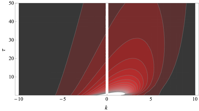
Figure 1: The function $F_{k}(\tau)$ given by (95) (with $\gamma=1$). The phase-mixing part of the spectrum is on the right ($k>0$), the anti-phase-mixing part on the left ($k<0$). The total energy is the sum and the Hermite flux the difference of these two. The broader-range scaling behaviour is better represented on a log scale: see figures 2 and 3.

Using (86) in (81) and changing the integration variable to $z=\xi^{2}/4(\sigma-\tau)$, we find

$$F^{-}(\tau,\xi)=\frac{1}{\Gamma\!\left(\frac{1}{3}\right)}\int_{0}^{\infty}\mathrm{d}z\,\frac{e^{-z}}{\left(\tau z+\frac{1}{4}\xi^{2}\right)^{2/3}}=\frac{e^{\xi^{2}/4\tau}}{\tau^{2/3}}\frac{\Gamma\!\left(\frac{1}{3};\frac{\xi^{2}}{4\tau}\right)}{\Gamma\!\left(\frac{1}{3}\right)}.$$ (92)

In the first of these expressions, both asymptotics (90) and (91) are manifest. In the second expression, which is obtained by changing the integration variable $z+\xi^{2}/4\tau\to z$,

$$\Gamma\!\left(\frac{1}{3};\frac{\xi^{2}}{4\tau}\right)=\int_{\xi^{2}/4\tau}^{\infty}\mathrm{d}z\,z^{-2/3}e^{-z}$$ (93)

is an upper incomplete gamma function.

Finally, using (91) and (86) in (76), we find

$$F^{+}(\tau,\xi) =\frac{e^{-\xi^{2}/4\tau}}{\tau^{2/3}}\left\{1+(-1)^{2/3}\Biggl{[}\frac{\Gamma\!\left(\frac{1}{3};-\frac{\xi^{2}}{4\tau}\right)}{\Gamma\!\left(\frac{1}{3}\right)}-1\Biggr{]}\right\}$$

$$=\frac{e^{-\xi^{2}/4\tau}}{\tau^{2/3}}\left[1+\frac{1}{\Gamma\!\left(\frac{1}{3}\right)}\int_{0}^{\xi^{2}/4\tau}\mathrm{d}z\,z^{-2/3}e^{z}\right].$$ (94)

The first term inside the bracket comes from the second integral in (76) (the boundary-value term) and is obtained by the manipulations analogous to those that led to (92). The second term comes from the first integral in (76) (the initial-value term), which is turned into a tabulated integral by changing the integration variable to $z=\xi\eta/2\tau$ (and then changing $z\to-z$ to obtain the last integral representation, which is perhaps more transparent than the one in terms of the incomplete gamma function).

5.3.2 Self-similar solution

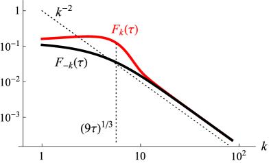
(a) $\tau=20$	(b) $k=7$

Figure 2: Typical cuts through the solution (95) (with $\gamma=1$) at (a) constant $\tau$, (b) constant $k$. The spectra of phase-mixing modes, $F_{k}(\tau)$, are shown in red and the spectra of anti-phase-mixing modes, $F_{-k}(\tau)$, in black. The asymptotic scalings (91) and (90) are shown for reference and convergence to them is manifest in the limits $k\gg(9\tau)^{1/3}$ and $\tau\gg k^{3}/9$, respectively. 2D plots of $F_{k}(\tau)$ and of the resulting Hermite flux and total energy spectrum are in figure 3.

Assembling (92) and (94) together and returning them to the original variables, we arrive at the following solution:

$$F_{k}(\tau)=\frac{e^{-k^{3}/9\gamma\tau}}{\tau^{2/3}}\left\{\begin{array}[]{l}\displaystyle 1+\frac{1}{\Gamma\!\left(\frac{1}{3}\right)}\int_{0}^{k^{3}/9\gamma\tau}\mathrm{d}z\,z^{-2/3}e^{z},\quad k>0,\\ \\ \displaystyle\frac{1}{\Gamma\!\left(\frac{1}{3}\right)}\int_{|k|^{3}/9\gamma\tau}^{\infty}\mathrm{d}z\,z^{-2/3}e^{-z},\quad k<0,\end{array}\right.$$ (95)

where $\tau=(2m)^{3/2}/3-\tau_{0}$ ($\tau_{0}$ is an order-unity offset). Hence the Fourier–Hermite spectrum $C_{k,m}$ and the Hermite flux $\Gamma_{k,m}$ can be calculated according to (49) and (50), respectively.

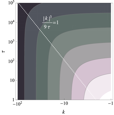
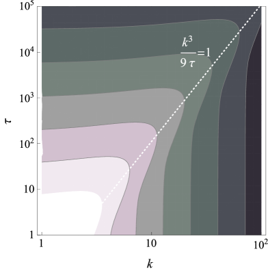
(a) $F_{k}(\tau)$, $k<0$	(b) $F_{k}(\tau)$, $k>0$
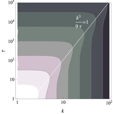
(c) $\bar{\Gamma}_{k}(\tau)$	(d) $\left[F_{k}(\tau)+F_{-k}(\tau)\right]/2$

Figure 3: (a,b) Same as figure 1, but on a log scale and across a broader range of $k$ and $\tau$. Note the asymptotic features (zero-flux solution, power-law scalings) discussed in sections 5.3.2 and 5.4. Cf. figure 4. (c) Normalised Hermite flux $\bar{\Gamma}$ defined by (96). Its contours are straight in the logarithmic coordinates because $\bar{\Gamma}=\bar{\Gamma}(k^{3}/9\tau)$. (d) Total energy spectrum $\left[F_{k}(\tau)+F_{-k}(\tau)\right]/2$ [see (49)].

The solution (95) is plotted in figure 1, which shows a pleasingly nontrivial shape. The essential result is, however, extremely simple. The solution is self-similar and could, in fact, have been obtained as such, by a shorter, if marginally less general, route (see appendix B). The similarity variable $k^{3}/9\gamma\tau$ determines the demarcation of the phase space into two asymptotic regions: the asymptotic of the spectrum when $|k|\gg(9\gamma\tau)^{1/3}$ is (91) and the asymptotic when $\tau\gg|k|^{3}/9\gamma$ is (90) [this is particularly obvious in the second expression in (81)]. The former describes fluctuations in the “wave-number inertial range” with a vanishing Hermite flux, the latter fluctuations in the “Hermite inertial range”, which also have zero Hermite flux. These scalings are illustrated in figure 2 and the normalised Hermite flux

$$\bar{\Gamma}=\frac{F_{k}(\tau)-F_{-k}(\tau)}{F_{k}(\tau)+F_{-k}(\tau)}=\frac{\Gamma_{k,m}}{\sqrt{2m}\,kC_{k,m}}$$ (96)

is plotted in figure 3(c). $\bar{\Gamma}$ is a good measure of how different the nonlinear state is from the linear one: for linear Landau-damped perturbations, we would have had $\bar{\Gamma}=1$ everywhere (Kanekar et al., 2015). Note that, as follows immediately from (95), $\bar{\Gamma}=\bar{\Gamma}(k^{3}/9\gamma\tau)$ is a function of the similarity variable only.

Another useful result is the overall Hermite spectrum integrated over all wave numbers. While this, of course, misses the relationship between structure in position and velocity space that we have focused on so closely, it is a good crude measure of how “phase-mixed” the distribution is (cf. Hatch et al., 2014; Servidio et al., 2017). So, from (49) and (95), after integrating out the self-similar functional dependence of $F_{k}(\tau)$ on $k^{3}/9\gamma\tau$, we deduce

$$\sum_{k}C_{k,m}=\sum_{k}\frac{F_{k}+F_{-k}}{2\sqrt{m}}\propto\frac{1}{m}.$$ (97)

This scaling—or, equivalently, the $k$-by-$k$ $C_{k,m}\propto m^{-3/2}$ scaling at large $m$ [see (90)],—being steeper than $m^{-1/2}$, implies that our solution does indeed decay fast enough in $m$ in order for the collisional dissipation to vanish at vanishing collisionality and so treating the collisionless limit as nonsingular was justified (see discussion in section 4.2). Still, restoring finite $\nu$ leads to a kind of “Kolmogorov scale” for our kinetic turbulence and to a quantitative measure of the applicability, or otherwise, of the linear approximation, so we are going to do this in section 5.4.

Finally, we may also calculate the overall wave-number spectrum of the free energy: again integrating out the self-similar functional dependence of $F_{k}(\tau)$, we get

$$\sum_{m}C_{k,m}\propto\frac{1}{k}.$$ (98)

Since the total variance of the perturbed distribution function is conserved in the Kraichnan–Kazantsev model (see section 4.2), the above result can be made made sense of as the classical Batchelor (1959) scaling of a passive scalar advected by a single-scale stochastic field.

5.4 Phase-space energy flows and role of collisions

The structure of our self-similar solution of (64) is, in fact, easily understood already by means of a qualitative examination of the equation, which is also a useful approach in evaluating the role of collisions. Figure 4 is a cartoon of phase-space energy flows in aid of the discussion that follows [cf. figure 3(a,b)].

5.4.1 Phase-mixing region

The phase-mixing term dominates over the nonlinearity when

$$\tau\ll\frac{k^{3}}{\gamma}\quad\Rightarrow\quad\frac{\partial F_{k}}{\partial\tau}=0,$$ (99)

so the solution is independent of $\tau$ in this region [see figure 3(b)]. This is the linear phase-mixing solution, $C_{k,m}\propto 1/\sqrt{m}$, obtained earlier by Zocco & Schekochihin (2011) and Kanekar et al. (2015). Its wave-number scaling, $F_{k}\propto 1/k^{2}$, is, however, a new feature, extracting which required matching with other regions.

A way of making sense of this solution is to go back to the time-dependent equation (46) [or (58)] and notice that, for $k>0$, whatever solution $\tilde{f}_{k}$ (and, therefore, $F_{k}$) exists at low $s$, it will propagate “upwards” (to higher $s$) along the characteristic

$$s=\frac{kt}{\sqrt{2}},$$ (100)

and it will do so unimpeded by the nonlinearity as long as the time $t$ is shorter than the nonlinear time $t_{\mathrm{nl}}$ associated with the mode-coupling term in the right-hand side of those equations. In the Kraichnan–Batchelor model,

$$t_{\mathrm{nl}}^{-1}\sim\frac{s^{2}\gamma}{k^{2}},\quad\gamma\sim p^{4}\varkappa_{p}\sim p^{4}\varphi_{p}^{2}t_{\mathrm{c}},$$ (101)

where $t_{\mathrm{c}}$ is the correlation time of the wave field $\varphi_{p}$ (effectively assumed to be single-scale). Requiring $t\ll t_{\mathrm{nl}}$ in (100), we see that the phase-mixing region of the phase space extends to $s^{3}\ll k^{3}/\gamma$, which is the same as the condition in (99).

This gives us a way to estimate how small the wave amplitude must be in order for the nonlinearity and associated effects never to matter: indeed, if the collision time is short compared to the nonlinear time,

$$t_{\nu}\sim\frac{1}{\nu s^{2}}\ll t_{\mathrm{nl}}\quad\Leftrightarrow\quad k\gg\left(\frac{\gamma}{\nu}\right)^{1/2}\equiv k_{\nu},$$ (102)

the phase-mixed distribution function will thermalise before the echo can bring any energy back from phase space. Putting $t_{\nu}$ into (100) tells us how far into phase space energy will travel:

$$\tau\sim s^{3}\ll\frac{k}{\nu}\equiv\tau_{\nu},\quad k\gg k_{\nu}.$$ (103)

Perhaps the most practically important conclusion from this is that, given the strength of the electric field and, therefore, via (101), the value of $\gamma$, we can predict the collisional cutoff wave number $k_{\nu}$, given by (102), at which phase mixing (Landau damping) curtails the universal spectrum that we have derived above: we shall see in a moment that for $k\gg k_{\nu}$, $\bar{\Gamma}=1$, i.e., there is no echo flux from high to low Hermite moments.

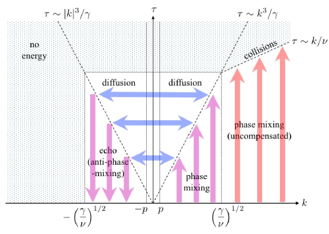
Figure 4: Cartoon of energy flows in phase space, including collisional cutoff. Cf. figure 3(a,b). Reminder: $\tau\sim m^{3/2}$ [see (59)] and $\gamma$ is related to the stochastic electric field via (101).

5.4.2 Diffusion and echo regions

Considering the limit opposite to (99), i.e., the region of phase space where $s\gg kt_{\mathrm{nl}}$, we get

$$\tau\gg\frac{k^{3}}{\gamma}\quad\Rightarrow\quad\frac{\partial^{2}F_{k}}{\partial k^{2}}=0,$$ (104)

i.e., $k$-space diffusion dominates. Our self-similar solution (section 5.3.2) tells us that the appropriate solution in this region is one independent of $k$ [see figures 3(b) and 3(a)] and $F_{k}(\tau)\propto 1/\tau^{2/3}$. This solution takes whatever values $F_{k}(\tau)$ has at $k\sim(\gamma\tau)^{1/3}$ [figure 3(b)] and transfers them across to $k\sim-(\gamma\tau)^{1/3}$ [figure 3(a)], where anti-phase-mixing picks them up and transfers them “downwards” to low Hermite moments ($\tau\to 0$), over times that are again shorter than $t_{\mathrm{nl}}$ (because $\tau\ll|k^{3}|/\gamma$ again), along the characteristic

$$s=s_{0}-\frac{|k|t}{\sqrt{2}},$$ (105)

where $s_{0}\sim\tau_{0}^{1/3}\sim|k|/\gamma^{1/3}$.

This last piece of the solution is the echo flux. It cancels the phase-mixing flux exactly, provided the energy ($F_{k}$) from $k>0$ has been successfully transferred by phase mixing from $\tau=0$ to $\tau\sim k^{3}/\gamma$ to be picked up by diffusion and carried over to the anti-phase-mixing region $k<0$. For $k\gg k_{\nu}$, the energy gets intercepted at $\tau\sim k/\nu$ [see (103)] and thermalised by collisions, so at $\tau\sim k^{3}/\gamma$, $F_{k}(\tau)=0$. This then gives $F_{-k}(0)=0$, i.e., no echo flux. Thus, $k_{\nu}$ is indeed the wave-number cutoff—a kind of “Kolmogorov scale” for Vlasov-kinetic turbulence—beyond which Landau damping can act as an efficient route to (eventually collisional) dissipation.

6 Discussion

6.1 Summary

We have considered what is arguably the simplest kinetic turbulence problem available: a 1D Vlasov–Poisson (section 2.1; or Vlasov–Boltzmann: see section 2.2) plasma with an energy source. When collisions are vanishingly weak, this gives rise to interesting dynamics across the 2D (position and velocity) phase space. In a simple approximation where the stochastic electric field mixing the particle distribution can be assumed to have statistics independent of the high-order moments of this distribution, a solvable model can be constructed in the same vein as the Kraichnan–Batchelor model used in the passive-scalar problem. The resulting analytical solution displays the same key features as have been surmised heuristically (Schekochihin et al., 2016) and found numerically (Parker et al., 2016) for plasma systems with higher-dimensional phase spaces (see section 6.2.5).

Namely, the free-energy flux from low to high Hermite moments is suppressed—i.e., the dissipation channel associated with Landau damping is shut down—for all wave numbers below a certain cut off $k_{\nu}=(\gamma/\nu)^{1/2}$ (see section 5.4). This cut off is a kinetic analog of the Kolmogorov scale: it scales inversely with the collision rate $\nu$ and increases with the amplitude of the electric perturbations—the latter determines $\gamma$, which is the rate of diffusion of the free energy in $k$ space due to the stochastic electric field. Thus, one might expect a kind of statistical “fluidisation” of the turbulence in the “inertial range” ($k\ll k_{\nu}$)—perhaps a welcome development from the point of view of the long history of attempts to reduce kinetics to fluid (or “Landau-fluid”) dynamics (see references and further discussion in section 6.2.4).

Expanding our interest beyond the effect of phase-space turbulence on the low (“fluid”) moments of the distribution function and to the structure of this turbulence across the (Fourier–Hermite) phase space, we find the latter cleanly partitioned into two regions: (i) the phase-mixing region $k\gtrsim\gamma^{1/3}\sqrt{m}$, where phase mixing and anti-phase-mixing transfer free energy between lower and higher Hermite moments (cancelling on average), and (ii) the mode-coupling (or diffusion) region $k\lesssim\gamma^{1/3}\sqrt{m}$, where the free energy is transferred between spatial scales (wave numbers) by the advecting action of the stochastic electric field. An overview of how this happens is provided in section 5.4 and figure 4, while the Fourier–Hermite spectrum is derived more formally in section 5 (summarised in section 5.3.2). The resulting scalings are

$$C_{m,k}\sim\left\{\begin{array}[]{ll}\displaystyle\frac{1}{\gamma^{2/3}m^{3/2}},&\displaystyle k\lesssim\gamma^{1/3}\sqrt{m},\quad m\ll\frac{\gamma^{1/3}}{\nu},\\ \\ \displaystyle\frac{1}{k^{2}\sqrt{m}},&\displaystyle\gamma^{1/3}\sqrt{m}\lesssim k\ll k_{\nu}=\left(\frac{\gamma}{\nu}\right)^{1/2}.\end{array}\right.$$ (106)

6.2 Open issues

There is a number of questions and lines of investigation that all this leaves open. The more immediate and obvious of them are, naturally, to do with how universal these results are, given the radical nature of the approximations that were made in order to obtain them, and how they can be made more general and more applicable to concrete physical problems. Let us itemise these questions briefly.

6.2.1 Multiscale electric fields

What happens outside Batchelor’s approximation (section 4.3), i.e., when the stochastic electric field cannot be treated as effectively single-scale and, therefore, as providing a diffusively accumulating series of small kicks in $k$ space to the perturbed distribution function? Formally, dealing with this issue is a matter of solving the integral equation (59), rather than the differential equation (64). A certain (limited) amount of progress on this is made in appendix A, suggesting somewhat steeper wave-number spectra in the mode-coupling region. While we do not have the full solution, it appears plausible that, even though scalings might change, the overall partitioning of the phase space into (anti-)phase-mixing- and mode-coupling-dominated regions should persist and the Landau damping would still be suppressed. In fact, the conversion between phase-mixing and anti-phase-mixing modes may be quicker in this case than in Batchelor’s limit because the steps in $k$ space need not be as small as in the diffusive regime (cf. Schekochihin et al., 2016).

6.2.2 Finite-time-correlated electric fields

What happens outside Krachnan’s approximation (section 4.1), i.e., if the assumption of a short correlation time of the electric field is relaxed? The experience of passive-advection problems in fluid dynamics (see, e.g., Antonsen Jr. et al., 1996; Bhat & Subramanian, 2015) suggests that generalising from white to finite-time-correlated advecting field rarely leads to dramatic qualitative changes. In the context of plasma kinetics, however, the limit, opposite to ours, of a long correlation time of the electric field clearly requires special care to capture the phase-space structure that will arise due to particle-trapping effects (Bernstein et al., 1957; O’Neil, 1965; O’Neil et al., 1971; Manheimer, 1971).

6.2.3 Self-consistent electric fields

How does one construct a fully nonlinear theory of kinetic turbulence, i.e., one in which the stochastic electric field is not prescribed but is determined self-consistently? This requires coupling the high-$m$ dynamics to the low-$m$ “fluid” equations derived in section 3.1, i.e., one would have to progress from the vague understanding that the flux to/from high Hermite moments is suppressed to a more quantitative model of how this suppression can be incorporated into a dynamical (“Landau fluid”; section 6.2.4) or, more likely, statistical model of the low-$m$ moments (and how many of them must be kept). Once this is done, it becomes possible to assess to what extent a self-consistent electric field can be compatible with the modelling choices made above: the Batchelor (single scale) and Kraichnan (short correlation time) approximations.

Without claiming to have such a theory, let us offer a few naïve but plausible estimates. Taking the limit of our solution at low $m$ [the second asymptotic in (106)], we find a $k^{-2}$ spectrum. Let us conjecture that this spectrum is established in phase space and imposes itself, via the linear Hermite coupling term in (29), on the lower Hermite moments. So, starting with (29) for $m=3$, we may predict

$$\langle|T_{k}|^{2}\rangle\equiv 2\langle|g_{k,2}|^{2}\rangle\sim\langle|g_{k,4}|^{2}\rangle\sim\langle|g_{k,6}|^{2}\rangle\sim\dots\sim k^{-2}.$$ (107)

From the wave equation (31) and in view of (30), we may estimate

$$n_{k}^{\pm}\sim\frac{k^{2}}{\omega_{k}^{2}}\,\theta_{k}=\frac{2}{3+\alpha_{k}}\,\theta_{k},\quad n_{k}\sim n_{k}^{\pm},\quad u_{k}\sim\frac{\omega_{k}}{k}\,n_{k}^{\pm}=\sqrt{\frac{3+\alpha_{k}}{2}}\,n_{k}^{\pm}.$$ (108)

Note that, regardless of the size of $\alpha_{k}$, $n_{k}$ is always either much smaller than or comparable to $\theta_{k}$. Therefore, $T_{k}=\theta_{k}+2n_{k}$ in (107) can be replaced by $\theta_{k}$ for the purposes of these crude estimates. This gives us a prediction for the spectra of the “wave quantities”:

$$\langle|n_{k}|^{2}\rangle\sim\left(\frac{2}{3+\alpha_{k}}\right)^{2}k^{-2},\quad\langle|u_{k}|^{2}\rangle\sim\frac{2}{3+\alpha_{k}}\,k^{-2}.$$ (109)

At wave numbers where, in (25), the self-consistent term ($\alpha_{k}\varphi_{k}$) dominates over the “external” one ($\chi_{k}$), the electric-field spectrum is

$$\langle|E_{k}|^{2}\rangle=k^{2}\langle|\varphi_{k}|^{2}\rangle\sim k^{2}\alpha_{k}^{2}\langle|n_{k}|^{2}\rangle\sim\left(\frac{2\alpha_{k}}{3+\alpha_{k}}\right)^{2}.$$ (110)

This tells us that, for example, for Vlasov–Poisson perturbations with $k\lambda_{\mathrm{D}e}\gg 1$ and $\alpha_{k}=2/k^{2}$ (see section 2.1), we should have $\langle|E_{k}|^{2}\rangle\sim k^{-4}$, which is a steep enough scaling to justify Batchelor’s approximation. In contrast, if $\alpha_{k}$ is a constant (ion-acoustic perturbations; see sections 2.2 and 2.3), the self-consistent $\langle|E_{k}|^{2}\rangle$ is flat (cut off at $k\sim k_{\nu}$) and our model can only work if the external potential $\chi_{k}$ plays the dominant part in the nonlinear mode coupling (in the case of ion-scale Zakharov turbulence, section 2.3, this might be a credible possibility as $\chi_{k}$ is fed by the fast-oscillating electric fields that satisfy an electron-time-scale fluid-like equation and have a tendency to form a large-scale condensate; see Zakharov 1972 and the reviews cited in section 2.3).

Finally, if one is interested in the stochastic-acceleration problem ($\alpha_{k}=0$; section 2.4), the electric field need not be self-consistent and the conclusion from the above considerations is that particles stochastically accelerated by a short-time-correlated electric field cut off above wave number $p$ will develop $k^{-2}$ density, velocity, temperature, etc.  spectra at $k\gg p$. This appears to be a new result.

The above discussion should probably not satisfy a discerning reader: clearly, there is much to be done before the link between the “kinetic” and “fluid” moments is established in an analytically solid and quantitative way.

6.2.4 Implications for Landau-fluid closures

The question of what constitutes a quantitatively accurate closure scheme for the first few fluid moments of a kinetic plasma system has been studied in some detail, both analytically and numerically, in the framework of “Landau-fluid” closures (Hammett & Perkins, 1990; Hammett et al., 1992, 1993; Dorland & Hammett, 1993; Beer & Hammett, 1996; Smith, 1997; Snyder et al., 1997; Passot & Sulem, 2004; Goswami et al., 2005; Tassi et al., 2016; Passot et al., 2017) and, indeed, by their detractors (e.g., Mattor, 1992; Weiland, 1992). A crude view of the philosophy behind this approach is that linear Landau-damping rates are incorporated explicitly into low-$m$ fluid equations to model the energy removal process into higher-order moments. This might appear to be inconsistent with the notion, advocated by us, that phase mixing is cancelled by anti-phase-mixing and thus Landau damping is effectively suppressed as a route to thermalisation of the low-$m$ energy. However, the situation is, in fact, more nuanced.

It was understood already in the course of development of early Landau-fluid models that their performance improves if more fluid moments are included. It was also understood that the cause of this improvement is that nonlinearities in those fluid equations act to reduce the phase-mixing rate to higher-order “unresolved” moments (Beer & Hammett, 1996; Smith, 1997). It seems plausible that keeping the “right” number of moments is tantamount to keeping enough $m$’s to enable the system to have enough anti-phase-mixing to capture the cancellation effect reasonably well—and that if the truncation is done at some $m$ that is still smaller than the $m$ at which the flux into higher-order moments is fully cancelled (which will depend on $k$), some form of Landau-fluid closure may be adequate to mop up the residual flux.

Furthermore, if the cut-ff scale $k_{\nu}$ is finite, i.e., if the collision rate is sufficiently large (equivalently, the velocity-space resolution of a code is limited) and/or the fluctuation amplitude is sufficiently small, the dissipation at $k\gtrsim k_{\nu}$ should be perfectly well described by the Landau rate corresponding to those $k$ (see section 5.4). We also saw (figure 3c) that, at least in our model, cancellation of the Hermite flux required $k\gg p$, i.e., worked in the “inertial range” ($p\ll k\ll k_{\nu}$), rather than at the “energy-containing scale” of the turbulence. It is easy to imagine situations (e.g., in near-marginal tokamak turbulence) in which the scale separation between $p$ and $k_{\nu}$ might not be large.

Thus, the usefulness of Landau-fluid closures, judiciously applied, is not obviated by the stochastic-echo effect—but it is clearly an interesting topic for exploration how the type of results reported above might help one hone these closures with this effect explicitly in one’s sights.

6.2.5 3D

What happens when the system is allowed to be 3D in both velocity and position space?

In magnetised, drift-kinetic plasmas, this, in fact, brings in only one extra phase-space variable ($k_{\perp}$ in addition to $k_{\parallel}$, all statistics being isotropic in the plane perpendicular to the magnetic field); phase mixing in drift kinetics is only in $v_{\parallel}$, so there is only one velocity-space dimension—provided the equilibrium is isotropic (if it is not, there is also phase-mixing in $v_{\perp}$; see Dorland & Hammett 1993, Mandell et al. 2017). The nonlinearity in a magnetised plasma is of a more traditional “fluid” type, viz., it is the advection of $\delta\!f$ by turbulent $\boldsymbol{E}\times\boldsymbol{B}$ flows. A certain amount of progress has been made (Hatch et al., 2014; Kanekar, 2015; Schekochihin et al., 2016; Parker et al., 2016) and is being made with this problem in application both to laboratory-inspired turbulence models and to the solar wind.

At scales where the finite size of particles’ Larmor orbits is felt, this triggers vigorous nonlinear phase mixing in $v_{\perp}$: the “entropy cascade” introduced by Schekochihin et al. (2008, 2009) (but anticipated already by Dorland & Hammett 1993) and first numerically diagnosed by Tatsuno et al. (2009) and Bañón Navarro et al. (2011) (see also Kawamori 2013, who claims experimental confirmation). Thus, gyrokinetic turbulence has a 5D phase space. Outside the gyrokinetic approximation, at high frequencies (comparable and exceeding the Larmor frequencies of the particles), the phase space finally becomes 6D, as the distribution function can develop structure also in the gyroangle.

In a recent promising development, the first harbinger has appeared (Servidio et al., 2017) of a stage in spacecraft exploration of plasma turbulence in the Earth’s magnetosphere and the solar wind when 3D Hermite spectra (and, perhaps, 6D Hermite–Fourier ones) become measurable and thus so much more attractive as a subject for theoretical prediction, now falsifiable (and not necessarily just Hermite spectra; see Howes et al. 2017 and Klein et al. 2017).

This is a good note to finish on: phase-space turbulence as a new frontier for observation and measurement, as well as theory—for we must hope that the phenomena that are revealed by simple solvable models of kinetic turbulence are not just interesting or aesthetically pleasing but also real.

Appendix A Solutions of (59) and the Batchelor approximation

Here we explore how the solutions of (59) might change if the electric-field correlation function $K_{p}=p^{2}\varkappa_{p}$ does not decay quickly enough in order for the Batchelor approximation [i.e., the expansion (63)] to be legitimate—and also under what condition on $K_{p}$ it is legitimate. Even if it cannot be turned into a differential operator, the mode-coupling integral in the right-hand side of (59) will, qualitatively, still provide a kind of smoothing effect in $k$ space (in the Batchelor limit, this was diffusion) and transfer $F_{k}$ from positive to negative wave numbers, causing anti-phase-mixing. One might again expect that this mode-coupling term will dominate over the phase-mixing term, $k\partial F_{k}/\partial\tau$, at sufficiently small $k$ and sufficiently large $\tau$, whereas in the opposite limit, the phase mixing (or anti-phase-mixing) will simply transfer energy “vertically” in the $(k,\tau)$ plane (analogously to figure 4). The solutions of (59) in the mode-coupling-dominated region will then be such functions $F_{k}$ that the right-hand side of (59) vanishes.

It is convenient to write this as follows, converting the wave-number sum into an integral

$$\int_{-\infty}^{+\infty}\mathrm{d}q\,K_{k-q}(F_{k}-F_{q})=0.$$ (111)

Let us assume that $K_{p}\propto|p|^{\alpha}$ and $F_{k}\propto|k|^{\beta}$. Scaling out $|k|^{\alpha+\beta+1}$ and changing the integration variable to $\xi=q/|k|$, we find that the above integral is proportional to

$$I=\int_{0}^{\infty}\mathrm{d}\xi\,(1-\xi^{\beta})\left(|1-\xi|^{\alpha}+|1+\xi|^{\alpha}\right).$$ (112)

The change of variables $\eta=1/\xi$ (a 1D Zakharov transformation; see Zakharov et al. 1992) turns this integral into

$$I=-\int_{0}^{\infty}\frac{\mathrm{d}\eta}{\eta^{2+\beta+\alpha}}(1-\eta^{\beta})\left(|1-\eta|^{\alpha}+|1+\eta|^{\alpha}\right).$$ (113)

This is just $-I$ and so $I=-I=0$, as required, if

$$\beta=-2-\alpha\quad\Rightarrow\quad F_{k}\propto|k|^{-2-\alpha}.$$ (114)

This is the desired solution satisfying (111). It is only valid provided the integral $I$ converges, the conditions for which are

$$\beta>-1,\quad-2<\alpha<-1\quad\Rightarrow\quad-1<\beta<0.$$ (115)

Otherwise, the integral (111) is dominated by what happens at the low- or high-wave-number cutoffs or at $|p|=|k-q|\ll|k|$ (i.e., $\xi\approx 1$).

The latter wave-number range ($|p|\ll|k|$) takes over the integral (111) for $\alpha\leq-2$. This corresponds to the flat solution ($\beta=0$) at $|k|\lesssim|p|$ that was derived in section 4.4 and that at $|k|\gg|p|$ transitions seamlessly into the Batchelor-limit solution worked out in section 5 (or appendix B). Thus, the condition of validity of the Batchelor approximation is that $K_{p}$ must certainly decay more steeply than $|p|^{-2}$.

Whether the shallow power-law solutions (114) have any interesting physical applications remains to be seen. Presumably, they indicate that when the Batchelor approximation is broken, the $k$ spectrum in the mode-coupling-dominated region becomes a little steeper than the flat Batchelor-limit solution—with some attendant change in the $\tau$ spectrum (and also in the $k$ spectrum in the phase-mixing-dominated region), to find which we would need to calculate the solution of (59) more precisely, taking into account the fact the power law (114) does not, in fact, extend to arbitrarily large $k$.

It is perhaps worth noting that these solutions must be rather particular to the 1D world, as wave-number integrals expressing nonlinear mode coupling become quite different in more dimensions (see, e.g., Zakharov et al., 1992).

Appendix B Self-similar solution of (64)

Consider (64) with $\nu=0$:

$$k\frac{\partial F_{k}}{\partial\tau}=\gamma\frac{\partial^{2}F_{k}}{\partial k^{2}}.$$ (116)

This equation has a self-similar solution of the form

$$F_{k}(\tau)=\frac{1}{\tau^{\lambda}}\,\Phi(\kappa),\quad\kappa=\frac{k^{3}}{\gamma\tau},$$ (117)

where $\Phi(\kappa)$ satisfies an ordinary differential equation readily obtained by substituting (117) into (116):

$$9\kappa\Phi^{\prime\prime}+(6+\kappa)\Phi^{\prime}+\lambda\Phi=0.$$ (118)

A standard method for fixing the exponent $\lambda$ for self-similar solutions such as (117) is to use some conservation law that the solution must satisfy. In this case, there is indeed a conservation law: (116) implies

$$\frac{\mathrm{d}}{\mathrm{d}\tau}\int_{-\infty}^{+\infty}\mathrm{d}k\,kF_{k}=0.$$ (119)

Using (117), we find

$$\int_{-\infty}^{+\infty}\mathrm{d}k\,kF_{k}=\frac{\tau^{\frac{2}{3}-\lambda}}{3}\int_{-\infty}^{+\infty}\mathrm{d}\kappa\,\kappa^{-1/3}\Phi(\kappa),$$ (120)

which would appear to require

$$\lambda=\frac{2}{3}$$ (121)

to make the integral (120) independent of $\tau$. In fact, we know from the argument in section 4.2 that this integral must be zero at $\tau\to 0$. In view of (119), it must then also be zero at all $\tau$. Thus, the choice of $\lambda=2/3$ cannot really be justified a priori, but it is intriguing because with this value, (118) is rendered easily solvable, so we will examine its consequences before discussing its legitimacy.

With $\lambda=2/3$, (118) is solved by the following substitution:

$$\psi=\Phi^{\prime}+\frac{1}{9}\Phi\quad\Rightarrow\quad\kappa\psi^{\prime}+\frac{2}{3}\psi=0\quad\Rightarrow\quad\psi=\frac{C_{1}}{|\kappa|^{2/3}},$$ (122)

where $C_{1}$ is an integration constant. Integrating again, we find

$$\Phi(\kappa)=e^{-\kappa/9}\left(C_{1}\int_{-\infty}^{\kappa}\mathrm{d}\kappa^{\prime}|\kappa^{\prime}|^{-2/3}e^{\kappa^{\prime}/9}+C_{2}\right),$$ (123)

where $C_{2}$ is another integration constant. It is clear that $C_{2}=0$, lest $\Phi(\kappa)$ blow up at $\kappa\to-\infty$. Cleaning up the remaining solution by changing the integration variable to $z=\kappa^{\prime}/9$, setting $C_{1}=\left[9^{1/3}\Gamma(1/3)\right]^{-1}$ (this is arbitrary and done for aesthetic reasons) and using the resulting $\Phi(\kappa)$ in (117), we arrive at the following solution

$$F_{k}(\tau)=\frac{e^{-k^{3}/9\gamma\tau}}{\tau^{2/3}}\frac{1}{\Gamma\!\left(\frac{1}{3}\right)}\int_{-\infty}^{k^{3}/9\gamma\tau}\mathrm{d}z\,|z|^{-2/3}e^{z}.$$ (124)

If we split the $k>0$ and $k<0$ cases explicitly, we recover the solution (95). It is a simple matter to ascertain that (124) has the asymptotics (90) and (91) when the similarity variable $k^{3}/9\gamma\tau$ is small or large, respectively. Indeed, changing the integration variable $z-k^{3}/9\gamma\tau\to-z$ in (124), we get

$$F_{k}(\tau)=\frac{1}{\Gamma\!\left(\frac{1}{3}\right)}\int_{0}^{\infty}\mathrm{d}z\,\frac{e^{-z}}{\bigl{|}\frac{1}{9\gamma}k^{3}-\tau z\bigr{|}^{2/3}}\to\left\{\begin{array}[]{ll}\displaystyle\frac{1}{\tau^{2/3}},&\displaystyle\frac{|k|^{3}}{9\gamma\tau}\ll 1,\\ \\ \displaystyle\frac{3^{4/3}}{\Gamma\!\left(\frac{1}{3}\right)}\frac{1}{k^{2}},&\displaystyle\frac{|k|^{3}}{9\gamma\tau}\gg 1.\end{array}\right.$$ (125)

This solution manifestly has vanishing Hermite flux ($F_{k}=F_{-k}$) at $\tau\ll|k^{3}|/9\gamma$ (as well as in the opposite limit, but this is just a trivial requirement of continuity of $F_{k}$ at $k=0$).

Obviously, the above derivation is much more elementary and may, to some readers, be more convincing than that offered in section 5. Methodologically, however, it was not necessarily obvious either that the self-similar solution would prove to be the only one that would have matching ($k$ by $k$) phase-mixing and anti-phase-mixing fluxes at $\tau\to 0$ or that this solution would be the only physically acceptable one. As we already indicated above, the choice of $\lambda=2/3$ was merely a convenient conjecture. In order to ascertain that it is the only possible choice, we would have to solve (118) for arbitrary $\lambda$ (which can be done in special functions) and then demand that the solutions are positive (i.e., represent physically realisable spectra) and satisfy (62). This can be done, but the argument for $\lambda=2/3$ given in appendix C is perhaps more mathematically compelling and at any rate no less cumbersome.

Admittedly, the formal shortcomings of the self-similar route to the answer are probably overcome by its appealing simplicity.

Appendix C Inevitability of the zero-flux solution (86)

Here we exercise due diligence by showing that the solution found in section 5, which we found using an initial guess (86), is indeed the only physically and mathematically sensible one.

Let us no longer make an explicit demand for a zero-flux solution, which led us from (83) to (85), the solution of which was (86). Instead of (86), let us posit some general power law for the Hermite spectrum at $\xi\to 0$:

$$Y(\tau)=\frac{1}{\tau^{\lambda}}.$$ (126)

With this ansatz, the left-hand side of (83) becomes

l.h.s. of (83) $$=\tau^{-\lambda-\frac{1}{3}}\Gamma\!\left(\frac{2}{3}\right)\left[\frac{\Gamma\!\left(\lambda+\frac{1}{3}\right)}{\Gamma(\lambda)}-\frac{\left(\lambda-\frac{2}{3}\right)\Gamma(1-\lambda)}{\Gamma\!\left(\frac{5}{3}-\lambda\right)}\right]$$ (127)

$$\quad+\underbrace{\frac{\mathrm{d}}{\mathrm{d}\tau}\,\tau^{\frac{2}{3}-\lambda}B\!\left(\frac{\tau}{\tau_{\mathrm{max}}};\lambda-\frac{2}{3},\frac{2}{3}\right)}_{\parbox{85.35826pt}{\begin{center}\small$\to 0$ as $\tau_{\mathrm{max}}\to\infty$\end{center}}},$$

where $B$ is the incomplete beta function. While the second integral in (83), equalling the expression under the derivative in (127), is divergent when $\lambda<2/3$ and $\tau_{\mathrm{max}}\to\infty$, its $\tau$ derivative vanishes in this limit and so the values $\lambda<2/3$ are formally allowed. The case $\lambda=2/3$ has to be treated differently, but has already been considered in section 5.3. Finally, we must have $\lambda<1$ in order to keep the first integral in (83) convergent.

To calculate the right-hand side of (83), we assume a general power law for the phase-mixing part of the Fourier spectrum at $\tau\to 0$,

$$F_{0}^{+}(\xi)=\frac{A}{\xi^{\mu}}=\left(\frac{3}{2}\right)^{\mu}\!\frac{A}{k^{3\mu/2}},$$ (128)

where $A$ is a constant, and find

$$\text{r.h.s. of (\ref{eq:flux_cont_sln})}=\tau^{-\frac{\mu}{2}-\frac{1}{3}}2^{-\mu}\Gamma\!\left(1-\frac{\mu}{2}\right)A.$$ (129)

In order for (83) to be satisfied, we must have

$$\lambda=\frac{\mu}{2}$$ (130)

and

$$A =2^{2\lambda}\Gamma\!\left(\frac{2}{3}\right)\left[\frac{\Gamma\!\left(\lambda+\frac{1}{3}\right)}{\Gamma(\lambda)\Gamma(1-\lambda)}-\frac{\lambda-\frac{2}{3}}{\Gamma\!\left(\frac{5}{3}-\lambda\right)}\right]$$

$$=2^{2\lambda}\Gamma\!\left(\frac{2}{3}\right)\frac{\lambda-\frac{2}{3}}{\Gamma\!\left(\frac{5}{3}-\lambda\right)}\left\{\frac{\sin\pi\lambda}{\sin\!\left[\pi\left(\lambda-\frac{2}{3}\right)\right]}-1\right\}.$$ (131)

The spectrum (128) must be positive: within our allowed interval $\lambda<1$, we can have $A>0$ only if $\lambda<5/6$.

Finally, via (84), the ansatz (126) implies that the anti-phase-mixing Fourier spectrum at $\tau\to 0$ is

$$F_{0}^{-}(\xi)=2^{2\lambda}\frac{\Gamma\!\left(\lambda+\frac{1}{3}\right)}{\Gamma\!\left(\frac{1}{3}\right)}\frac{1}{\xi^{2\lambda}}.$$ (132)

(the integral is done by changing the integration variable to $z=\xi^{2}/4\sigma$). In view of (130), this is the same scaling as for the phase-mixing spectrum (128)! But this means that the condition (62) can only be satisfied if the coefficients in (132) and (128) match. With $A$ given by (131), this leads us, therefore, to demand

$$A=2^{2\lambda}\frac{\Gamma\!\left(\lambda+\frac{1}{3}\right)}{\Gamma\!\left(\frac{1}{3}\right)}\quad\Leftrightarrow\quad\cos\!\left[\pi\!\left(\lambda-\frac{1}{3}\right)\right]=\frac{1}{2}.$$ (133)

This is satisfied for $\lambda=2/3$, which hands us back our zero-flux solution (86) and everything that it implies.

The reason that this has proved to be the only physically acceptable possibility is that for any $0<\lambda<2/3$, we would have $F_{0}^{+}>F_{0}^{-}$ and their wave-number scaling would be shallower than $1/k^{2}$, causing the integral in (62) to blow up. For $2/3<\lambda<5/6$, the integral is finite but negative, meaning that there is no steady state and there is an unphysical net inflow of energy from high $m$. For even larger values of $\lambda$, either there is no positive spectrum at all or the energy flux through $k=0$ blows up. Finally, $\lambda=0$ is not allowed because, even though (133) and so (62) are satisfied, the right-hand side of (61) no longer vanishes at $\nu\to+0$ and so the steady-state energy budget breaks down, i.e., no such steady-state solution can exist—this is a demonstration that the linear Hermite solution does not work in a nonlinear steady state.

References

- Antonsen Jr. et al. (1996) Antonsen Jr., T. M., Fan, Z., Ott, E. & Garcia-Lopez, E. 1996 The role of chaotic orbits in the determination of power spectra of passive scalars. Phys. Fluids 8, 3094.
- Bañón Navarro et al. (2011) Bañón Navarro, A., Morel, P., Albrecht-Marc, M., Carati, D., Merz, F., Görler, T. & Jenko, F. 2011 Free energy cascade in gyrokinetic turbulence. Phys. Rev. Lett. 106, 055001.
- Batchelor (1959) Batchelor, G. K. 1959 Small-scale variation of convected quantities like temperature in turbulent fluid. Part 1. General discussion and the case of small conductivity. J. Fluid Mech. 5, 113.
- Beer & Hammett (1996) Beer, M. A. & Hammett, G. W. 1996 Toroidal gyrofluid equations for simulations of tokamak turbulence. Phys. Plasmas 3, 4046.
- Bernstein et al. (1957) Bernstein, I. B., Greene, J. M. & Kruskal, M. D. 1957 Exact nonlinear plasma oscillations. Phys. Rev. 108, 546.
- Bhat & Subramanian (2015) Bhat, P. & Subramanian, K. 2015 Fluctuation dynamos at finite correlation times using renewing flows. J. Plasma Phys. 81, 395810502.
- Boldyrev & Cattaneo (2004) Boldyrev, S. & Cattaneo, F. 2004 Magnetic-field generation in Kolmogorov turbulence. Phys. Rev. Lett. 92, 144501.
- Cook (1978) Cook, I. 1978 Application of the Novikov-Furutsu theorem to the random acceleration problem. Plasma Phys. 20, 349.
- Davidson (2004) Davidson, P. A. 2004 Turbulence: An Introduction for Scientists and Engineers. Oxford: Oxford University Press.
- Dorland & Hammett (1993) Dorland, W. & Hammett, G. W. 1993 Gyrofluid turbulence models with kinetic effects. Phys. Fluids B 5, 812.
- Dupree (1972) Dupree, T. H. 1972 Theory of phase space density granulation in plasma. Phys. Fluids 15, 334.
- Falkovich et al. (2001) Falkovich, G., Gawȩdzki, K. & Vergassola, M. 2001 Particles and fields in fluid turbulence. Rev. Mod. Phys. 73, 913.
- Furutsu (1963) Furutsu, K. 1963 On the statistical theory of electromagnetic waves in a fluctuating medium (I). J. Res. NBS 67D, 303.
- Goldman (1984) Goldman, M. V. 1984 Strong turbulence of plasma waves. Rev. Mod. Phys. 56, 709.
- Goswami et al. (2005) Goswami, P., Passot, T. & Sulem, P. L. 2005 A Landau fluid model for warm collisionless plasmas. Phys. Plasmas 12, 102109.
- Gould et al. (1967) Gould, R. W., O’Neil, T. M. & Malmberg, J. H. 1967 Plasma wave echo. Phys. Rev. Lett. 19, 219.
- Hammett et al. (1993) Hammett, G. W., Beer, M. A., Dorland, W., Cowley, S. C. & Smith, S. A. 1993 Developments in the gyrofluid approach to tokamak turbulence simulations. Plasma Phys. Control. Fusion 35, 973.
- Hammett et al. (1992) Hammett, G. W., Dorland, W. & Perkins, F. W. 1992 Fluid models of phase mixing, Landau damping, and nonlinear gyrokinetic dynamics. Phys. Fluids B 4, 2052.
- Hammett & Perkins (1990) Hammett, G. W. & Perkins, F. W. 1990 Fluid moment models for Landau damping with application to the ion-temperature-gradient instability. Phys. Rev. Lett. 64, 3019.
- Hatch et al. (2014) Hatch, D. R., Jenko, F., Bratanov, V. & Bañón Navarro, A. 2014 Phase space scales of free energy dissipation in gradient-driven gyrokinetic turbulence. J. Plasma Phys. 80, 531.
- Howes et al. (2017) Howes, G. G., Klein, K. G. & Li, T. C. 2017 Diagnosing collisionless energy transfer using field-particle correlations: Vlasov-Poisson plasmas. J. Plasma Phys. 83, 705830102.
- Kanekar et al. (2015) Kanekar, A., Schekochihin, A. A., Dorland, W. & Loureiro, N. F. 2015 Fluctuation-dissipation relations for a plasma-kinetic Langevin equation. J. Plasma Phys. 81, 305810104.
- Kanekar (2015) Kanekar, A. V. 2015 Phase mixing in turbulent magnetized plasmas. Ph. D. Thesis. University of Maryland, College Park (URL: http://drum.lib.umd.edu/handle/1903/16418).
- Kawamori (2013) Kawamori, E. 2013 Experimental verification of entropy cascade in two-dimensional electrostatic turbulence in magnetized plasma. Phys. Rev. Lett. 110, 095001.
- Kazantsev (1968) Kazantsev, A. P. 1968 Enhancement of a magnetic field by a conducting fluid. Sov. Phys.–JETP 26, 1031.
- Kingsep (2004) Kingsep, A. S. 2004 Introduction to Nonlinear Plasma Physics. Moscow: MZ Press (in Russian).
- Klein et al. (2017) Klein, K. G., Howes, G. G. & Tenbarge, J. M. 2017 Diagnosing collisionless energy transfer using field-particle correlations: gyrokinetic turbulence. J. Plasma Phys. 83, 535830401.
- Knorr (1977) Knorr, G. 1977 Time asymptotic statistics of the Vlasov equation. J. Plasma Phys. 17, 553.
- Kosuga & Diamond (2011) Kosuga, Y. & Diamond, P. H. 2011 On relaxation and transport in gyrokinetic drift wave turbulence with zonal flow. Phys. Plasmas 18, 122305.
- Kosuga et al. (2014) Kosuga, Y., Itoh, S.-I., Diamond, P. H., Itoh, K. & Lesur, M. 2014 Ion temperature gradient driven turbulence with strong trapped ion resonance. Phys. Plasmas 21, 102303.
- Kosuga et al. (2017) Kosuga, Y., Itoh, S.-I., Diamond, P. H., Itoh, K. & Lesur, M. 2017 Role of phase space structures in collisionless drift wave turbulence and impact on transport modeling. Nucl. Fusion 57, 072006.
- Kraichnan (1968) Kraichnan, R. H. 1968 Small-scale structure of a scalar field convected by turbulence. Phys. Fluids 11, 945.
- Kraichnan (1974) Kraichnan, R. H. 1974 Convection of a passive scalar by a quasi-uniform random straining field. J. Fluid Mech. 64, 737.
- Kraichnan (1994) Kraichnan, R. H. 1994 Anomalous scaling of a randomly advected passive scalar. Phys. Rev. Lett. 72, 1016.
- Krommes (1997) Krommes, J. A. 1997 The clump lifetime revisited: Exact calculation of the second-order structure function for a model of forced, dissipative turbulence. Phys. Plasmas 4, 655.
- Krommes (2015) Krommes, J. A. 2015 A tutorial introduction to the statistical theory of turbulent plasmas, a half-century after Kadomtsev’s Plasma Turbulence and the resonance-broadening theory of Dupree and Weinstock. J. Plasma Phys. 81, 205810601.
- Landau (1946) Landau, L. 1946 On the vibration of the electronic plasma. Zh. Eksp. Teor. Fiz. 16, 574.
- Laval et al. (2016) Laval, G., Pesme, D. & Adam, J.-C. 2016 Wave-particle and wave-wave interactions in hot plasmas: a French historical point of view. Eur. Phys. J. H, doi: 10.1140/epjh/e2016-70050-2 .
- Lenard & Bernstein (1958) Lenard, A. & Bernstein, I. B. 1958 Plasma oscillations with diffusion in velocity space. Phys. Rev. 112, 1456.
- Lesur et al. (2014a) Lesur, M., Diamond, P. H. & Kosuga, Y. 2014a Nonlinear current-driven ion-acoustic instability driven by phase-space structures. Plasma Phys. Control. Fusion 56, 075005.
- Lesur et al. (2014b) Lesur, M., Diamond, P. H. & Kosuga, Y. 2014b Phase-space jets drive transport and anomalous resistivity. Phys. Plasmas 21, 112307.
- Malmberg et al. (1968) Malmberg, J. H., Wharton, C. B., Gould, R. W. & O’Neil, T. M. 1968 Plasma wave echo experiment. Phys. Rev. Lett. 20, 95.
- Mandell et al. (2017) Mandell, N. R., Dorland, W. & Landreman, M. 2017 Laguerre-Hermite pseudo-spectral velocity formulation of gyrokinetics. J. Plasma Phys., submitted [arXiv:1708.04029] .
- Manheimer (1971) Manheimer, W. M. 1971 Strong turbulence theory of nonlinear stabilization and harmonic generation. Phys. Fluids 14, 579.
- Manheimer & Dupree (1968) Manheimer, W. M. & Dupree, T. H. 1968 Weak turbulence theory of velocity space diffusion and the nonlinear Landau damping of waves. Phys. Fluids 11, 2709.
- Mattor (1992) Mattor, N. 1992 Can Landau-fluid models describe nonlinear Landau damping? Phys. Fluids B 4, 3952.
- Mazitov (1965) Mazitov, R. K. 1965 Damping of plasma waves. J. Appl. Mech. Tech. Phys. 6, 22.
- Musher et al. (1995) Musher, S. L., Rubenchik, A. M. & Zakharov, V. E. 1995 Weak Langmuir turbulence. Phys. Rep. 252, 177.
- Novikov (1965) Novikov, E. A. 1965 Functionals and the random-force method in turbulence theory. Sov. Phys.–JETP 20, 1290.
- O’Neil (1965) O’Neil, T. 1965 Collisionless damping of nonlinear plasma oscillations. Phys. Fluids 8, 2255.
- O’Neil et al. (1971) O’Neil, T. M., Winfrey, J. H. & Malmberg, J. H. 1971 Nonlinear interaction of a small cold beam and a plasma. Phys. Fluids 14, 1204.
- Orszag & Kraichnan (1967) Orszag, S. A. & Kraichnan, R. H. 1967 Model equations for strong turbulence in a Vlasov plasma. Phys. Fluids 10, 1720.
- Parker & Dellar (2015) Parker, J. T. & Dellar, P. J. 2015 Fourier-Hermite spectral representation for the Vlasov-Poisson system in the weakly collisional limit. J. Plasma Phys. 81, 305810203.
- Parker et al. (2016) Parker, J. T., Highcock, E. G., Schekochihin, A. A. & Dellar, P. J. 2016 Suppression of phase mixing in drift-kinetic plasma turbulence. Phys. Plasmas 23, 070703.
- Passot & Sulem (2004) Passot, T. & Sulem, P. L. 2004 A Landau fluid model for dispersive magnetohydrodynamics. Phys. Plasmas 11, 5173.
- Passot et al. (2017) Passot, T., Sulem, P. L. & Tassi, E. 2017 Electron-scale reduced fluid models with gyroviscous effects. J. Plasma Phys. 83, 715830402.
- Plunk et al. (2010) Plunk, G. G., Cowley, S. C., Schekochihin, A. A. & Tatsuno, T. 2010 Two-dimensional gyrokinetic turbulence. J. Fluid Mech. 664, 407.
- Plunk & Tatsuno (2011) Plunk, G. G. & Tatsuno, T. 2011 Energy transfer and dual cascade in kinetic magnetized plasma turbulence. Phys. Rev. Lett. 106, 165003.
- Robinson (1997) Robinson, P. A. 1997 Nonlinear wave collapse and strong turbulence. Rev. Mod. Phys. 69, 507.
- Rudakov & Tsytovich (1978) Rudakov, L. I. & Tsytovich, V. N. 1978 Strong Langmuir turbulence. Phys. Rep. 40, 1.
- Schekochihin (2017) Schekochihin, A. A. 2017 Lecture Notes on Kinetic Theory and Magnetohydrodynamics of Plasmas. URL: http://www-thphys.physics.ox.ac.uk/people/AlexanderSchekochihin/KT/2015/KTLectureNotes.pdf.
- Schekochihin et al. (2008) Schekochihin, A. A., Cowley, S. C., Dorland, W., Hammett, G. W., Howes, G. G., Plunk, G. G., Quataert, E. & Tatsuno, T. 2008 Gyrokinetic turbulence: a nonlinear route to dissipation through phase space. Plasma Phys. Control. Fusion 50, 124024.
- Schekochihin et al. (2009) Schekochihin, A. A., Cowley, S. C., Dorland, W., Hammett, G. W., Howes, G. G., Quataert, E. & Tatsuno, T. 2009 Astrophysical gyrokinetics: kinetic and fluid turbulent cascades in magnetized weakly collisional plasmas. Astrophys. J. Suppl. 182, 310.
- Schekochihin et al. (2004a) Schekochihin, A. A., Cowley, S. C., Taylor, S. F., Maron, J. L. & McWilliams, J. C. 2004a Simulations of the small-scale turbulent dynamo. Astrophys. J. 612, 276.
- Schekochihin et al. (2004b) Schekochihin, A. A., Haynes, P. H. & Cowley, S. C. 2004b Diffusion of passive scalar in a finite-scale random flow. Phys. Rev. E 70, 046304.
- Schekochihin et al. (2007) Schekochihin, A. A., Iskakov, A. B., Cowley, S. C., McWilliams, J. C., Proctor, M. R. E. & Yousef, T. A. 2007 Fluctuation dynamo and turbulent induction at low magnetic Prandtl numbers. New J. Phys. 9, 300.
- Schekochihin et al. (2016) Schekochihin, A. A., Parker, J. T., Highcock, E. G., Dellar, P. J., Dorland, W. & Hammett, G. W. 2016 Phase mixing versus nonlinear advection in drift-kinetic plasma turbulence. J. Plasma Phys. 82, 905820212.
- Servidio et al. (2017) Servidio, S., Chasapis, A., Matthaeus, W. H., Perrone, D., Valentini, F., Parashar, T. N., Veltri, P., Gershman, D., Russell, C. T., Giles, B., Fuselier, S. A., Phan, T. D. & Burch, J. 2017 Magnetospheric Multiscale (MMS) observation of plasma velocity-space cascade: Hermite representation and theory. Phys. Rev. Lett. 119, 205101.
- Smith (1997) Smith, S. A. 1997 Dissipative closures for statistical moments, fluid moments, and subgrid scales in plasma turbulence. Ph. D. Thesis. Princeton University (URL: http://w3.pppl.gov/~hammett/sasmith/thesis.html).
- Snyder et al. (1997) Snyder, P. B., Hammett, G. W. & Dorland, W. 1997 Landau fluid models of collisionless magnetohydrodynamics. Phys. Plasmas 4, 3974.
- Sturrock (1966) Sturrock, P. A. 1966 Stochastic acceleration. Phys. Rev. 141, 186.
- Sutton (1943) Sutton, W. G. L. 1943 On the equation of diffusion in a turbulent medium. Proc. R. Soc. London A 182, 48.
- Tassi et al. (2016) Tassi, E., Sulem, P. L. & Passot, T. 2016 Reduced models accounting for parallel magnetic perturbations: gyrofluid and finite Larmor radius-Landau fluid approaches. J. Plasma Phys. 82, 705820601.
- Tatsuno et al. (2009) Tatsuno, T., Dorland, W., Schekochihin, A. A., Plunk, G. G., Barnes, M., Cowley, S. C. & Howes, G. G. 2009 Nonlinear phase mixing and phase-space cascade of entropy in gyrokinetic plasma turbulence. Phys. Rev. Lett. 103, 015003.
- Teaca et al. (2012) Teaca, B., Bañón Navarro, A., Jenko, F., Brunner, S. & Villard, L. 2012 Locality and universality in gyrokinetic turbulence. Phys. Rev. Lett. 109, 235003.
- Teaca et al. (2016) Teaca, B., Bañón Navarro, A., Told, D. & Jenko, F. 2016 Kinetic intermittency in magnetized plasma turbulence. E-print arXiv:1607.03421 .
- Thornhill & ter Haar (1978) Thornhill, S. G. & ter Haar, D. 1978 Langmuir turbulence and modulational instability. Phys. Rep. 43, 43.
- Tsytovich (1995) Tsytovich, V. N. 1995 Lectures on Non-linear Plasma Kinetics. Berlin: Springer.
- Vedenov et al. (1962) Vedenov, A. A., Velikhov, E. P. & Sagdeev, R. Z. 1962 Quasilinear theory of plasma oscillations. Nucl. Fusion Suppl., Part 2 p. 465.
- Watanabe & Sugama (2004) Watanabe, T.-H. & Sugama, H. 2004 Kinetic simulation of steady states of ion temperature gradient driven turbulence with weak collisionality. Phys. Plasmas 11, 1476.
- Weiland (1992) Weiland, J. 1992 Nonlinear effects in velocity space and drift wave transport in tokamaks. Phys. Fluids B 4, 1388.
- Zakharov (1972) Zakharov, V. E. 1972 Collapse of Langmuir waves. Sov. Phys.–JETP 35, 908.
- Zakharov et al. (1992) Zakharov, V. E., L’vov, V. S. & Falkovich, G. 1992 Kolmogorov Spectra of Turbulence I: Wave Turbulence. Berlin: Springer.
- Zakharov et al. (1985) Zakharov, V. E., Musher, S. L. & Rubenchik, A. M. 1985 Hamiltonian approach to the description of non-linear plasma phenomena. Phys. Rep. 129, 285.
- Zeldovich et al. (1990) Zeldovich, Ya. B., Ruzmaikin, A. A. & Sokoloff, D. D. 1990 The Almighty Chance. Singapore: World Scientific.
- Zocco & Schekochihin (2011) Zocco, A. & Schekochihin, A. A. 2011 Reduced fluid-kinetic equations for low-frequency dynamics, magnetic reconnection, and electron heating in low-beta plasmas. Phys. Plasmas 18, 102309.