Data Discovery and Anomaly Detection Using Atypicality: Signal Processing Methods

Abstract

The aim of atypicality is to extract small, rare, unusual and interesting pieces out of big data. This complements statistics about typical data to give insight into data. In order to find such “interesting” parts of data, universal approaches are required, since it is not known in advance what we are looking for. We therefore base the atypicality criterion on codelength. In a prior paper we developed the methodology for discrete-valued data, and the the current paper extends this to real-valued data. This is done by using minimum description length (MDL). We show that this shares a number of theoretical properties with the discrete-valued case. We develop the methodology for a number of “universal” signal processing models, and finally apply them to recorded hydrophone data.

I Introduction

One characteristic of the information age is the exponential growth of information, and the ready availability of this information through networks, including the internet – “Big Data.” The question is what to do with this enormous amount of information. One possibility is to characterize it through statistics – think averages. The perspective in this paper is the opposite, namely that most of the value in the information is in the parts that deviate from the average, that are unusual, atypical. The rest is just background noise. Take art: the truly valuable paintings are those that are rare and atypical. The same could be true for scientific research and entrepreneurship.

The aim of our approach is to extract such ’rare interesting’ data out of big data sets. The central question is what ’interesting’ means. A first thought is to focus on the ’rare’ part. That is, interesting data is something that is unlikely based on prior knowledge of typical data or examples of typical data, i.e., training. This is the way an outlier is usually defined. Unlikeliness could be measured in terms of likelihood or according to some distance measure. This is also the most common principle in anomaly detection [1]. However, perhaps being unlikely is not sufficient for something to be ’interesting.’ In many cases, outliers are junk that are eliminated not to contaminate the typical data. What makes something interesting is perhaps that it has a new unusual structure in itself that is quite different than the structure of the data we have already seen. Return to the example of paintings: what make masterworks interesting is not just that they are different than other paintings, but that they have some ’structure’ that is intriguing. Or take another example. Many scientific discoveries, like the theory of relativity and quantum mechanics, began with experiments that did not fit with prevailing theories. The experiments were outliers or anomalies. What made them truly interesting was that it was possible to find a new theory to explain the data, be it relativity or quantum mechanics. This is the principle we pursue: finding data that have better alternative explanations than those that fit the typical data.

In the paper [2] we used this intuition to develop a methodology, atypicality, that can be used to discover such data. The basic idea is that if some data can be encoded with a shorter codelength in itself, i.e., with a universal source coder, rather than using the optimum coder for typical data, then it is atypical. The purpose of the current paper is to generalize this to real-valued data. Lossless source coding does not generalize directly to real-valued data. Instead we can use minimum description length (MDL). In the current paper we develop an approach to atypicality based on MDL, and show its usefulness on a real dataset.

II Atypicality

We repeat the argumentation for atypicality from [2]. Our starting point is the in theory of randomness developed by Kolmogorov and Martin-Löf [3, 4]. Kolmogorov divides (infinite) sequences into ’typical’ and ’special.’ The typical sequences are those that we can call random, that is, they satisfy all laws of probability. They can be characterized through Kolmogorov complexity. A sequence of bits $\{x_{n},n=1,\ldots,\infty\}$ is random (i.e, iid uniform) if the Kolmogorov complexity of the sequence satisfies $K(x_{1},\ldots,x_{n})\geq n-c$ for some constant $c$ and for all $n$ [3]. The sequence is incompressible if $K(x_{1},\ldots,x_{n}|n)\geq n$ for all $n$, and a finite sequence is algorithmically random if $K(x_{1},\ldots,x_{n}|n)\geq n$ [4]. In terms of coding, an iid random sequence is also incompressible, or, put another way, the best coder is the identity function. Let us assume we draw sequences $x^{n}$ from an iid uniform distribution. The optimum coder is the identity function, and the code length is $n$. Now suppose that for one of these sequences we can find a (universal) coder so that the code length is less than $n$; while not directly equivalent, one could state this as $K(x_{1},\ldots,x_{n}|n)<n$. With an interpretation of Kolmogorov’s terms, this would not be a ’typical’ sequence, but a ’special’ sequence. We will instead call such sequences ’atypical.’ Considering general distributions and general (finite) alphabets instead of iid uniform distributions, we can state this in the following general principle [2]

Definition 1.

A sequence is atypical if it can be described (coded) with fewer bits in itself rather than using the (optimum) code for typical sequences.

III Real-valued models

We would like to extend definition 1 and the approach in [2] to real-valued models. The approach in [2] can at a high level be described as comparing a typical coder based on fixed codes (e.g., Huffman codes for given probabilities) with an atypical coder based on a universal source coder; if the universal code is shorter, the sequence is declared atypical. As in [2] we would like to locate fixed length sequences, variable length sequences, and subsequences of variable length.

The definition is based on exact description of data, and lossless source coding rather than lossy (rate-distortion) therefore is the appropriate generalization. Lossless coding of real-valued data is used in many applications, for example lossless audio coding [5]. Direct encoding of the reals represented as binary numbers, such as done in lossless audio coding, makes the methods too dependent on data representation rather than the underlying data. Instead we will use a more abstract model of (finite-precision) reals. We will assume a fixed point representation with a (large) finite number, $r$, bits after the period, and an unlimited number of bits prior to the period [6]. Assume that the actual data is distributed according to a pdf $f(x)$. Then the number of bits required to represent $x$ is given by

$$L(x) =-\log\int_{x}^{x+2^{-r}}f(t)dt\approx-\log(f(x)2^{-r})$$

$$=-\log(f(x))+r$$ (1)

As we are only interested in comparing codelengths the dependency on $r$ cancels out. Suppose we want to decide between two models $f_{1}(x)$ and $f_{2}(x)$ for data. Then we decide $f_{1}(x)$ if $\lim_{r\to\infty}-\log\int_{x}^{x+2^{-r}}f_{1}(t)dt+\log\int_{x}^{x+2^{-r}}f_{2}(t)dt>0$, which is $-\log f_{1}(x)>-\log f_{2}(x)$. Thus for the typical codelength we can simply use $L_{t}(x)=-\log f(x)$, where $f(x)$ is the known distribution of typical data. One can also argue for this codelength more fundamentally from finite blocklength rate-distortion in the limit of low distortion [7]. Notice that this codelength is not scaling invariant:

$$y =ax+b$$

$$L_{t}(y) =-\log f(x)+\log|a|$$ (2)

which means care has to be taken when transforms of data are considered.

For the atypical codelength, there is nothing like universal source coding for the reals. The principle of universal source coding is that the transmitted sequence allows decoding of both the sequence and potential unknown parameters (this is the idea in the CTW algorithm [8] used in [2]). That principle is similar to that used in Rissanen’s minimum description length (MDL) [6]. The MDL is generally a codelength based on a specific model; on the other hand, in atypicality we are not interested in finding out if the data follows a specific model. Therefore, our approach is to try to code the data with a set of various general data (signal processing) models hoping that one of them approximates the actual model of the data better than the typical model. Let the models be $\mathcal{M}_{i,k}$, where the first index denotes the model type and the second index the number of (real) parameters. The atypical codelength for a sequence $x^{l}=\{x_{1},x_{2},\ldots,x_{l}\}$ then is

$$L_{a}(x^{l})=\min_{i,k}L(x^{l}|\mathcal{M}_{i,k})+L(i,k)$$ (3)

where $L(x^{l}|\mathcal{M}_{i,k})$ is the codelength to encode $x^{l}$ with the model $\mathcal{M}_{i,k}$ including any parameters and $L(i,k)$ is some code to tell the decoder which model is used. An even better approach is to use weighting as in [8],

$$L_{a}(x^{l})=-\log\left(\sum_{i,k}w_{i,k}2^{-L(x^{l}|\mathcal{M}_{i,k})}\right),$$

where $\sum_{i,k}w_{i,k}\leq 1$. A central tenet of atypicality is an adherence to strict decodability: we imagine that there is a receiver that receives solely a sequence of bits, and from this it should be able to reconstruct the data. Thus, the codelengths $L(x^{l}|\mathcal{M}_{i,k})$ should be actual lengths. On the other hand, strict universality (as in for example normalized maximum likelihood [9]) is less central. Even if each code $L(x^{l}|\mathcal{M}_{i,k})$ satisfies some strict universality criterion, the final codelength $L_{a}(x^{l})$ might not necessarily satisfy this. So, universality in some vague sense is sufficient.

The most common application of MDL is model selection and choosing number of parameters in the model. Thus, two codelengths $L(x^{l}|\mathcal{M}_{i,k})$ and $L(x^{l}|\mathcal{M}_{\tilde{i},\tilde{k}})$ are compared. In atypicality, on the other hand, the MDL codelength is only compared to the typical codelength $L_{t}(x^{l})$. This has a number of consequences. First, we might use different MDL methods for different models – this makes little sense in model selection, but perfect sense in atypicality. Second, we might use different models for different parts of the sequence $x^{l}$. Finally, again strict universality is less important.

In atypicality, as mentioned at the start of the section, we are also interested in finding sequences of variable length. It is therefore important that any MDL principle used works for both short and long sequences.

IV Minimum Description Length (MDL)

Let $f(x^{l}|\boldsymbol{\theta})$ denote a pdf for the sequence $x^{l}$ parametrized the $k$-dimensional parameter vector $\boldsymbol{\theta}$. Rissanen’s famous MDL approach [6] is a way to jointly encode the sequence $x^{l}$ and the unknown parameters $\boldsymbol{\theta}$. A widely known expression for codelength, frequently used in signal processing, is

$$L=-\log f(x^{l}|\hat{\boldsymbol{\theta}})+\frac{k}{2}\log l$$ (4)

where $\hat{\boldsymbol{\theta}}$ is the maximum likelihood (ML) estimate. The expression (4) is known to be a quite good approximation for many actual MDL coding methods [9], e.g., within an $O(1)$ term under some restrictive assumptions.

One possible approach to generalizing atypicality to real-valued data is therefore to simply use the expression (4) as the atypical codelength. This has the advantage that we can easily take any signal processing model, count the number of unknown parameters, and then use (4); we believe this is a valid approach to atypicality. It also had the advantage that it is possible to derive analytical results, see Section IV-B.

However, the issue is still that (4) is not a true codelength. As mentioned in Section III, a tenet of atypicality is to use actual codelength; additionally, we would like to analyze sequences of variable length $l$, where perhaps even $k$ is increasing with $l$. We would also like to apply atypicality to mixed type data that has both discrete and real components. The discrete coder returns an actual codelength, so that is better combined with an actual real-valued codelength. More generally, when combining multiple methods as in (3), the arbitrary constant in (4) (or terms of order less than $\log l$) influences detection and false alarm probabilities critically, and this gives issues with using (4). Finally (4) is difficult to directly apply when using transform-coding as in Sections V-C and VI-D.

For use in atypicality we therefore introduce two new MDL methods, based on a common principle. Our starting point is Rissanen’s [10] original predictive MDL

$$L(x^{l})=-\sum_{i=0}^{l-1}\log f(x_{i+1}|\boldsymbol{\hat{\theta}}(x^{i}))$$ (5)

The issue with this method is how to initialize the recursion. When $i=0$, $\boldsymbol{\hat{\theta}}(x^{i})$ is not defined. Rissanen suggests using a default pdf $f_{d}$ to encode data until $\boldsymbol{\hat{\theta}}(x^{i})$ is defined, so that $L(x^{l})=-\sum_{i=1}^{l-1}\log f(x_{i+1}|\boldsymbol{\hat{\theta}}(x^{i}))-\log f_{d}(x_{1})$. In general, with more than one parameter, the default pdf might have to be used for more samples. The remaining issue is that even when $\boldsymbol{\hat{\theta}}(x^{i})$ is defined, the estimate might be poor, and using this in (5) can give very long codelengths, see Fig. 1 below. Our solution is rather than using the ML estimate for encoding as though it is the actual parameter value, we use it as an uncertain estimate of $\boldsymbol{\theta}$. We then take this uncertainty into account in the codelength. This is similar to the idea of using confidence intervals in statistical estimates [11]. Below we introduce two methods using this general principle. This is different than the sequentially normalized maximum likelihood method [12], which modifies the encoder itself.

IV-A Subsequences

As in [2] our main interest is to find atypical subsequences of long sequences. The main additional consideration here is that when an atypical subsequence is encoded, the decoder also needs to know the start and end of the sequence. As described in [2], the start is encoded with a special codeword of length $\tau$ bits, where $\tau\approx-\log P(\text{\text{'atypical'})}$, and the end is encoded by transmitting the length of the sequence, which [6, 13] can be done with $\log^{*}l+\log c$, where $c$ is a constant and $\log^{*}(l)=\log l+\log\log l+\log\log\log l+\cdots$. If we use (4) only the first term matters, and we get a subsequence codelength

$$L=-\log f(x^{l}|\hat{\boldsymbol{\theta}})+\frac{k+2}{2}\log l+\tau$$ (6)

In principle the term $\tau$ does not matter as there are unknown constants, but $\tau$ is useful as a threshold. As shown in [2] the extra $\log l$ term is essential to obtain a finite atypical subsequence probability. In the following we will principally consider the subsequence problem.

IV-B Asymptotic MDL

In this section we assume (6) is used as codelength. Developing algorithms is straightforward: we just use various maximum likelihood estimators and count the number of parameters. Examples can be found in [14]. Here we will focus on performance analysis.

Consider a simple example. The typical model is a pure zero-mean Gaussian noise model with known variance $\sigma^{2}$. For the atypical model we let $x\sim\mathcal{N}(\mu_{a},\sigma^{2}$) with $\mu_{a}$ unknown. The typical codelength is

$$L_{t}(l) =-\sum\log\left(\frac{1}{\sqrt{2\pi\sigma^{2}}}\exp\left(-\frac{x[n]^{2}}{2\sigma^{2}}\right)\right)$$

$$=\frac{l}{2}\log 2\pi\sigma^{2}+\sum\frac{x[n]^{2}}{2\sigma^{2}\ln 2}$$

The ML estimate of the one unknown parameter $\mu_{a}$ is the average $\bar{x}$, and we get a codelength using (6)

$$L_{a}(l) =\frac{l}{2}\log 2\pi\sigma^{2}+\sum\frac{\left(x[n]-\bar{x}\right)^{2}}{2\sigma^{2}\ln 2}+\frac{3}{2}\log l+\tau$$

The criterion for atypicality is

$$L_{t}(l)-L_{a}(l)=\frac{l\bar{x}^{2}}{2\sigma^{2}\ln 2}-\frac{3}{2}\log l-\tau>0$$

or

$$\left|\frac{1}{\sqrt{l}}\sum x[n]\right|>\sigma\sqrt{3\ln l+(2\tau+5)\ln 2}$$

If the data is typical, $\frac{1}{\sqrt{l}}\sum x[n]\sim\mathcal{N}(0,\sigma^{2})$. Of key theoretical interest is the probability that a sequence generated according to the typical model is classified is atypical. One can think of this as a false alarm, but since the sequence is indistinguishable from one generated from an alternative model, we prefer the term intrinsically atypical [2].

The probability of a sequence being intrinsically atypical is upper bounded by [15]

$$P_{A}(l) =2Q\left(\sqrt{3\ln l+(2\tau+5)\ln 2}\right)$$

$$\leq\exp\left(-(3\ln l+(2\tau+5)\ln 2)/2\right)$$

$$=2^{-5/2}l^{-3/2}2^{-\tau}.$$

and lower bounded by

$$P_{A}(l) >\frac{2}{\sqrt{2\pi(3\ln l+(2\tau+5)\ln 2)}}\left(1-\frac{1}{3\ln l+(2\tau+5)\ln 2}\right)$$

$$\times\exp\left(-(3\ln l+(2\tau+5)\ln 2)/2\right)$$

from which we conclude

$$\lim_{l\to\infty}\frac{\ln P_{A}(l)}{-\frac{3}{2}\ln l}=1$$ (7)

It is interesting that this is the same expression (except for constant factors) as for the iid binary case in [2]. It means that, using the Gaussian mean criterion is equivalent to using the binary criterion on the sign of the samples. This illustrates that the discrete version of atypicality and real-valued version are part of one unified theory.

For the general vector Gaussian case, we have the following result

Theorem 2.

Suppose that the typical model is $\mathcal{N}(\mathbf{s},\boldsymbol{\Sigma})$ and the atypical model is $\mathcal{N}(\mathbf{s}(\boldsymbol{\theta}),\boldsymbol{\Sigma}(\boldsymbol{\theta}))$, where $\boldsymbol{\theta}$ is $k$-dimensional. Then the probability $P_{A}(l)$ of an intrinsically atypical subsequence is bounded by

$$\limsup_{l\to\infty}\frac{\ln P_{A}(l)}{-\frac{k+2}{2}\ln l}\leq 1$$ (8)

Proof:

For simplicity of notation, in this proof we will assume codelength is in nats and use natural logarithms throughout. We can precode the data with the typical model, so that after precoding we can assume the typical model is $\mathcal{N}(0,\mathbf{I}).$ The atypicality criterion is

$$r(\mathbf{x})=-\ln\frac{f(\mathbf{x}|\hat{\boldsymbol{\theta})}}{f(\mathbf{x})}\geq\tau+\frac{k+2}{2}\ln l$$

The Chernoff bound now states that for any $s>0$

$$P\left(r(\mathbf{x})\geq\tau+\frac{k+2}{2}\ln l\right) \leq\exp(-s(\tau+\frac{k+2}{2}\ln l))M_{r}(s)$$

where $M_{r}(s)=E[e^{sr}]$. If we put $s=1$ we obtain (8), provided $M_{r}(s)$ is bounded as $l\to\infty$. We will prove that $M_{r}(s)\leq K<\infty$ independent of $l$ for any $s<1$, which is sufficient to state (8) by letting $s\to 1$ sufficiently slow as $l\to\infty$.

We have

$$-\ln\frac{f(\mathbf{x}|\hat{\boldsymbol{\theta})}}{f(\mathbf{x})} =\frac{1}{2}\sum_{n=1}^{l}\mathbf{x}_{n}^{T}\mathbf{x}_{n}$$

$$-\frac{1}{2}\sum_{n=1}^{l}\left(\mathbf{x}_{n}-\mathbf{s}(\hat{\boldsymbol{\theta}})\right)^{T}\boldsymbol{\hat{\Sigma}}(\boldsymbol{\theta})^{-1}\left(\mathbf{x}_{n}-\mathbf{s}(\hat{\boldsymbol{\theta}})\right)$$

$$-\frac{l}{2}\ln\det\boldsymbol{\hat{\Sigma}}(\boldsymbol{\theta})$$

We need to upper bound this expression. Maximum likelihood estimation is given by minimizing the second and third terms over all $(\mathbf{s}(\hat{\boldsymbol{\theta}}),\boldsymbol{\hat{\Sigma}}(\boldsymbol{\theta})),\boldsymbol{\theta}\in\mathbb{R}^{k}$. The set $(\mathbf{s}(\hat{\boldsymbol{\theta}}),\boldsymbol{\hat{\Sigma}}(\boldsymbol{\theta})),\boldsymbol{\theta}\in\mathbb{R}^{k}$ is a manifold in $\mathbb{R}^{M}\times\mathbb{R}^{M^{2}}$. Minimizing over all (valid) vectors $\mathbb{R}^{M}\times\mathbb{R}^{M^{2}}\in\mathbb{R}^{M}$ can only make the term smaller, and the minimizer is of course the ML estimate, here $\mathbf{y}=(\hat{\boldsymbol{\mu}},\hat{\boldsymbol{\Sigma}})$ with $\hat{\boldsymbol{\mu}}=\frac{1}{l}\sum_{i=1}^{l}\mathbf{x}_{i}$, $\hat{\boldsymbol{\Sigma}}=\frac{1}{l}\sum_{i-1}^{l}(\mathbf{x}_{i}-\hat{\boldsymbol{\mu}})(\mathbf{x}_{i}-\hat{\boldsymbol{\mu}})^{T}$. Thus

$$-\ln\frac{f(\mathbf{x}|\hat{\boldsymbol{\theta})}}{f(\mathbf{x})} \leq\frac{1}{2}\sum_{n=1}^{l}\mathbf{x}_{n}^{T}\mathbf{x}_{n}$$

$$-\frac{1}{2}\sum_{n=1}^{l}\left(\mathbf{x}_{n}-\hat{\boldsymbol{\mu}}\right)^{T}\hat{\boldsymbol{\Sigma}}^{-1}\left(\mathbf{x}_{n}-\hat{\boldsymbol{\mu}}\right)-\frac{l}{2}\ln\det\boldsymbol{\hat{\Sigma}}$$

$$=\frac{1}{2}\sum_{n=1}^{l}\mathbf{x}_{n}^{T}\mathbf{x}_{n}-\frac{lM}{2}-\frac{l}{2}\ln\det\boldsymbol{\hat{\Sigma}}$$

$$=\frac{l}{2}\text{tr}\boldsymbol{\hat{\Sigma}}-\frac{lM}{2}-\frac{l}{2}\ln\det\boldsymbol{\hat{\Sigma}}+\frac{l}{2}\hat{\boldsymbol{\mu}}^{T}\hat{\boldsymbol{\mu}}$$

and

$$E[e^{sr}] \leq E\left[\exp\left(\frac{sl}{2}\text{tr}\boldsymbol{\hat{\Sigma}}-\frac{slM}{2}-\frac{sl}{2}\ln\det\boldsymbol{\hat{\Sigma}}\right)\exp\left(\frac{sl}{2}\hat{\boldsymbol{\mu}}^{T}\hat{\boldsymbol{\mu}}\right)\right]$$

$$\leq E\left[\exp\left(\frac{sl}{2}\text{tr}\boldsymbol{\hat{\Sigma}}-\frac{slM}{2}-\frac{sl}{2}\ln\det\boldsymbol{\hat{\Sigma}}\right)\right]$$

$$\times E\left[\exp\left(\frac{sl}{2}\hat{\boldsymbol{\mu}}^{T}\hat{\boldsymbol{\mu}}\right)\right]$$ (9)

For the latter expectation we use that $\hat{\boldsymbol{\mu}}\sim\mathcal{N}(0,\frac{1}{l}\mathbf{I})$. We can therefore write

$$E\left[\exp\left(\frac{sl}{2}\hat{\boldsymbol{\mu}}^{T}\hat{\boldsymbol{\mu}}\right)\right] \leq\frac{\sqrt{l}}{(2\pi)^{l/2}}\int\exp\left(\frac{sl}{2}\mathbf{t}^{T}\mathbf{t}\right)\exp\left(-\frac{l}{2}\mathbf{t}^{T}\mathbf{t}\right)d\mathbf{t}$$

$$\leq K$$

for $s<1$.

We rewrite the first expectation in (9) as

$$E\left[\exp\left(\frac{sl}{2}\text{tr}\boldsymbol{\hat{\Sigma}}-\frac{slM}{2}-\frac{sl}{2}\ln\det\boldsymbol{\hat{\Sigma}}\right)\right]$$

$$=E\left[\exp\left(\frac{sl}{2}\text{tr}\left(\frac{(l-1)}{(l-1)}\boldsymbol{\hat{\Sigma}}\right)-\frac{slM}{2}-\frac{sl}{2}\ln\det\left(\frac{(l-1)}{(l-1)}\boldsymbol{\hat{\Sigma}}\right)\right)\right]$$

$$=E\left[\exp\left(\frac{sl}{2(l-1)}\text{tr}\boldsymbol{\Sigma}-\frac{slM}{2}-\frac{sl}{2}\ln\left(\frac{1}{(l-1)^{M}}\det\boldsymbol{\Sigma}\right)\right)\right]$$

$$=E\left[\exp\left(\frac{sl}{2(l-1)}\text{tr}\boldsymbol{\Sigma}-\frac{slM}{2}+\frac{slM}{2}\ln\left(l-1\right)-\frac{sl}{2}\ln\det\boldsymbol{\Sigma}\right)\right]$$

Here $\boldsymbol{\Sigma}=(l-1)\hat{\boldsymbol{\Sigma}}$ , which is known to have a Wishart distribution $\mathcal{W}_{M}(\mathbf{I},l-1)$ [16] with pdf

$$f(\boldsymbol{\Sigma})=\frac{1}{2^{(l-1)M/2}\Gamma_{M}(\frac{l-1}{2})}\left(\det\boldsymbol{\Sigma}\right)^{(l-M-2)/2}\exp\left(-\frac{1}{2}\text{tr}\boldsymbol{\Sigma}\right)$$

The expectation can now be evaluated as the integral

$$I =\alpha\int_{\boldsymbol{\Sigma}>0}\exp\left(\frac{s\frac{l}{l-1}-1}{2}\text{tr}\boldsymbol{\Sigma}\right)\left(\det\boldsymbol{\Sigma}\right)^{((1-s)l-M-2)/2}d\boldsymbol{\Sigma}$$

$$=\alpha\Gamma_{M}\left(\frac{(1-s)l-1}{2}\right)\left(\frac{s\frac{l}{l-1}-1}{2}\right)^{-M((1-s)l-M-2)/2-1}$$

where $\alpha$ is a factor independent of $\boldsymbol{\Sigma}$

$$\alpha =\frac{\left(l-1\right)^{\frac{slM}{2}}\exp\left(-\frac{slM}{2}\right)}{2^{(l-1)M/2}\Gamma_{M}(\frac{l-1}{2})}$$

and $\Gamma_{M}$ is the multivariate gamma function [16]. Using Stirling’s approximation repeatedly, and performing some lengthy but straightforward simplifications we then get

$$I \sim\left(\frac{(1-s)l-1}{l-1}\right)^{M(1-M)/2}$$

$$\leq K$$

when $s<1$.

∎

Corollary 3.

Suppose that we consider a finite set of atypical signal models $\{\mathbf{s}(\boldsymbol{\theta}),\boldsymbol{\Sigma}(\boldsymbol{\theta})\}$. Then

$$\limsup_{l\to\infty}\frac{\ln P_{A}(l)}{-\frac{3}{2}\ln l}\leq 1$$

Proof:

We can use the union bound over the different models. The models with slowest decay in $l$ will dominate for large $l$, and these are exactly the one-parameter models. ∎

On the other hand, we know from (7) that for the simple mean, the probability of an atypical sequence is exactly $\sim l^{-3/2}$. Thus, adding more complex models will not change this by the Corollary. This is the benefit of using MDL: searching over very complex models will not increase the probability of intrinsically atypical sequences, or in terms of anomaly detection, the false alarm probability.

IV-C Normalized Likelihood Method (NLM)

As explained previously, our approach to predictive MDL is to introduce uncertainty in the estimate of $\boldsymbol{\theta}$. The first method is very simple. Let the likelihood function of the model be $f(x^{l}|\boldsymbol{\theta})$. For a fixed $x^{l}$ we can consider this as a “distribution” on $\boldsymbol{\theta}$; the ML estimate is of course the most likely value of this distribution. To account for uncertainty in the estimate, we can instead try use the total $f(x^{l}|\boldsymbol{\theta})$ to give a distribution on $\boldsymbol{\theta}$, and then use this for prediction. In general $f(x^{l}|\boldsymbol{\theta})$ is not a probability distribution as it does not integrate to 1 in $\boldsymbol{\theta}$. We can therefore normalize it to get a probability distribution

$$f_{x^{l}}(\boldsymbol{\theta})=\frac{f(x^{l}|\boldsymbol{\theta})}{C(x^{l})};\quad C(x^{l})=\int f(x^{l}|\boldsymbol{\theta})d\boldsymbol{\theta}$$ (10)

if $\int f(x^{l};\boldsymbol{\theta})d\boldsymbol{\theta}$ is finite. For comparison, the Bayes posteriori distribution is

$$f(\boldsymbol{\theta}|x^{l})=\frac{f(x^{l}|\boldsymbol{\theta})f(\boldsymbol{\theta)}}{\int f(x^{l}|\boldsymbol{\theta})f(\boldsymbol{\theta)}d\boldsymbol{\theta}}$$

If the support $\Theta$ of $\boldsymbol{\theta}$ has finite area, (10) is just the Bayes predictor with uniform prior. If the support $\Theta$ of $\boldsymbol{\theta}$ does not have finite area, we can get (10) as a limiting case when we take the limit of uniform distributions on finite $\Theta_{n}$ that converge towards $\Theta$. This is the same way the ML estimator can be seen as a MAP estimator with uniform prior [17]. One can reasonably argue that if we have no further information about $\boldsymbol{\theta}$, a uniform distribution seems reasonable, and has indeed been used for MDL [9] as well as universal source coding [4, Section 13.2]. What the Normalized Likelihood Method does is simply extend this to the case when there is no proper uniform prior for $\boldsymbol{\theta}$.

The method was actually implicitly mentioned as a remark by Rissanen in [18, Section 3.2], but to our knowledge was never further developed; the main contribution in this paper is to introduce the method as a practical method. From Rissanen we also know the coding distribution for $x_{n}$

$$f(x_{n+1}|x^{n})=\int f(x_{n+1}|\boldsymbol{\theta})f_{x^{n}}(\boldsymbol{\theta})d\boldsymbol{\theta}=\frac{C\left(x^{n+1}\right)}{C\left(x^{n}\right)}$$ (11)

Let us assume $C(x^{n})$ becomes finite for $n>1$ (this is not always the case, often $n$ needs to be larger). The total codelength can then be written as

$$L(x^{l}) =\sum_{i=1}^{l-1}-\log f(x_{i+1}|x^{i})-\log f_{d}(x_{1})$$

$$=-\log C(x^{l})+\log C(x^{2})-\log f_{d}(x_{1})$$ (12)

IV-D Sufficient Statistic Method (SSM)

The second method for introducing uncertainty in the estimate of $\boldsymbol{\theta}$ is more intricate. It is best explained through a simple example. Suppose our model is $\mathcal{N}(\mu,\sigma^{2})$, with $\sigma$ known. The average $\bar{x}_{n}$ is the ML estimate of $\mu$ at time $n$. We know that

$$\bar{x}_{n}=\mu+z,\quad z\sim\mathcal{N}\left(0,\frac{\sigma^{2}}{n}\right).$$

We can re-arrange this as

$$\mu=\bar{x}_{n}-z$$

Thus, given $\bar{x}_{n}$, we can think of $\mu$ as random $\mathcal{N}\left(\bar{x}_{n},\frac{\sigma^{2}}{n}\right)$. Now

$$x_{n+1}=\mu+z_{n+1}\sim\mathcal{N}\left(\bar{x}_{n},\sigma^{2}+\frac{\sigma^{2}}{n}\right)$$

which we can use as a coding distribution for $x_{n+1}$. This compares to $\mathcal{N}\left(\bar{x}_{n},\sigma^{2}\right)$ that we would use in traditional predictive MDL. Thus, we have taken into account that the estimate of $\mu$ is uncertain for $n$ small. The idea of thinking of the non-random parameter $\mu$ as random is very similar to the philosophical argument for confidence intervals [11].

In order to generalize this example to more complex models, we take the following approach. Suppose $\mathbf{t}(x^{n})$ is a $k$-dimensional sufficient statistic for the $k$-dimensional $\boldsymbol{\theta}\in\Theta$. Also suppose there exists some function $\mathbf{s}$ and a $k$-dimensional (vector) random variable $\mathbf{Y}$ independent of $\boldsymbol{\theta}$ so that

$$\mathbf{t}(x^{n})=\mathbf{s}(\mathbf{Y},\boldsymbol{\theta}).$$ (13)

We now assume that for every $(\mathbf{t},\mathbf{Y})$ in their respective support (13) has a solution for $\boldsymbol{\theta}\in\Theta$ so that we can write

$$\boldsymbol{\theta}=\mathbf{r}(\mathbf{Y},\mathbf{t}(x^{n})).$$ (14)

The parameter $\boldsymbol{\theta}$ is now a random variable (assuming $\mathbf{r}$ is measurable, clearly) with a pdf $f_{x^{n}}(\boldsymbol{\theta})$ This then gives a distribution on $x_{n+1}$, i.e.,

$$f(x_{n+1}|x^{n}) =\int f(x_{n+1}|\boldsymbol{\theta})f_{x^{n}}(\boldsymbol{\theta})d\boldsymbol{\theta}$$ (15)

The method has the following property

Theorem 4.

The distribution of $x_{n+1}$ is invariant to arbitrary parameter transformations.

This is a simple observation from the fact that (15) is an expectation, and that when $\boldsymbol{\theta}$ is transformed, the distribution according to (14) is also transformed with the same function.

One concern is the way the method is described. Perhaps we could use different functions $\mathbf{s}$ and $\mathbf{r}$ and get a different result? In the following we will prove that the distribution of $\boldsymbol{\theta}$ is independent of which $\mathbf{s}$ and $\mathbf{r}$ are used.

It is well-known [19, 4] that if the random variable $X$ has CDF $F$, then $U=F(X)$ has a uniform distribution (on $[0,1]$). Equivalently, $X=F^{-1}(U)$ for some uniform random variable $U$. We need to generalize this to $n$ dimensions. Recall that for a continuous random variable [19]

$$F_{i|i-1,\ldots,1}(x_{i}|x_{i-1},\ldots x_{1})=\int_{-\infty}^{x_{i}}f(t|x_{i-1},\ldots,x_{1})dt$$

$$=\frac{1}{f(x_{i-1},\ldots,x_{1})}\int_{-\infty}^{x_{i}}f(t,x_{i-1},\ldots,x_{1})dt$$

whenever $f(x_{i-1},\ldots,x_{1})\neq 0$. As an example, let $n=2$. Then the map $(X_{1},X_{2})\mapsto(F_{1}(X_{1}),F_{2|1}(X_{2},X_{1}))$ is a map from $\mathbb{R}^{2}$ onto $[0,1]^{2}$, and $(F_{1}(X_{1}),F_{2|1}(X_{2},X_{1}))$ has uniform distribution on $[0,1]^{2}$. Here $F_{1}(X_{1})$ is continuous in $X_{1}$ and $F_{2|1}(X_{2},X_{1})$ is continuous in $X_{2}$

We can write $X_{1}=F_{1}^{-1}(U_{1})$. For fixed $x_{1}$ we can also write $X_{2}=F_{2|1}^{-1}(U_{2}|x_{1})$ for those $x_{1}$ where $F_{2|1}$ is defined, and where the inverse function is only with respect to the parameter before $|$. Then

$$\left[\begin{array}[]{c}X_{1}\\ X_{2}\end{array}\right]=\left[\begin{array}[]{c}F_{1}^{-1}(U_{1})\\ F_{2|1}^{-1}(U_{2}|F_{1}^{-1}(U_{1}))\end{array}\right]\triangleq\check{\mathbf{F}}^{-1}(U_{1},U_{2})$$

This gives the correct joint distribution on $(X_{1},X_{2})$: the marginal distribution on $X_{1}$ is correct, and the conditional distribution of $X_{2}$ given $X_{1}$ is also correct, and this is sufficient. Clearly $\check{\mathbf{F}}^{-1}$ is not defined for all $U_{1},U_{2}$; the relationship should be understood as being valid for almost all $(X_{1},X_{2})$ and $(U_{1},U_{2})$. We can now continue like this for $X_{3},X_{4},\ldots,X_{n}$. We will state this result as a lemma

Lemma 5.

For any continuous random variable $\mathbf{X}$ there exists an $n$-dimensional uniform random variable $\mathbf{U}$, so that $\mathbf{X}=\check{\mathbf{F}}^{-1}(\mathbf{U})$.

Theorem 6.

Consider a model $\mathbf{t}=\mathbf{s}_{1}(\mathbf{Y}_{1};\boldsymbol{\theta}),$ with $\boldsymbol{\theta}=\mathbf{r}_{1}(\mathbf{Y}_{1};\mathbf{t})$ and an alternative model $\mathbf{t}=\mathbf{s}_{2}(\mathbf{Y}_{2};\boldsymbol{\theta}),$ with $\boldsymbol{\theta}=\mathbf{r}_{2}(\mathbf{Y}_{2};\mathbf{t}).$ We make the following assumptions

1. The support of $\mathbf{t}$ is independent of $\boldsymbol{\theta}$ and its interior is connected.

2. The extended CDF $\check{\mathbf{F}}_{i}$ of $\mathbf{Y}_{i}$ is continuous and differentiable.

3. The function $\mathbf{Y}_{i}\mapsto\mathbf{s}_{i}(\mathbf{Y}_{i};\boldsymbol{\theta})$ is one-to-one, continuous, and differentiable for fixed $\boldsymbol{\theta}$.

Then the distributions of $\boldsymbol{\theta}$ given by $\mathbf{r}_{1}$ and $\mathbf{r}_{2}$ are identical.

Proof:

By Lemma 5 write $\mathbf{Y}_{1}=\mathbf{F}_{1}^{-1}(\mathbf{U}_{1})$, $\mathbf{Y}_{2}=\mathbf{F}_{2}^{-1}(\mathbf{U}_{2})$. Let $u$ be the $k$-dimensional uniform pdf, i.e, $u(\mathbf{x})=1$ for $\mathbf{x}\in[0,1]^{k}$ and 0 otherwise, and let $\mathbf{Y}_{i}=\mathbf{s}_{i}^{-1}(\mathbf{t};\boldsymbol{\theta})$ denote the solution of $\mathbf{t}=\mathbf{s}_{i}(\mathbf{Y}_{i};\boldsymbol{\theta})$ with respect to $\mathbf{Y}_{i}$, which is a well-defined due to assumption 3. We can then write the distribution of $\mathbf{t}$ in two ways as follows ([19]), due to the differentiability assumptions

$$f(\mathbf{t};\boldsymbol{\theta}) =u(\mathbf{F}_{1}(\mathbf{s}_{1}^{-1}(\mathbf{t};\boldsymbol{\theta}))\left|\frac{\partial\mathbf{F}_{1}(\mathbf{s}_{1}^{-1}(\mathbf{t};\boldsymbol{\theta})}{\partial\mathbf{t}}\right|$$

$$=u(\mathbf{F}_{2}(\mathbf{s}_{2}^{-1}(\mathbf{t};\boldsymbol{\theta}))\left|\frac{\partial\mathbf{F}_{2}(\mathbf{s}_{2}^{-1}(\mathbf{t};\boldsymbol{\theta})}{\partial\mathbf{t}}\right|$$

Due to assumption 1 we can then that conclude $\frac{\partial\mathbf{F}_{1}(\mathbf{s}_{1}^{-1}(\mathbf{t};\boldsymbol{\theta})}{\partial\mathbf{t}}=\frac{\partial\mathbf{F}_{2}(\mathbf{s}_{2}^{-1}(\mathbf{t};\boldsymbol{\theta})}{\partial\mathbf{t}}$, or

$$\mathbf{F}_{1}(\mathbf{s}_{1}^{-1}(\mathbf{t};\boldsymbol{\theta})=\mathbf{F}_{2}(\mathbf{s}_{2}^{-1}(\mathbf{t};\boldsymbol{\theta}))+\mathbf{k}(\boldsymbol{\theta})$$

But both $\mathbf{F}_{1}$ and $\mathbf{F}_{2}$ have range $[0,1]^{k}$, and it follows that $\mathbf{k}(\boldsymbol{\theta})=\mathbf{0}$. Therefore

$$\mathbf{t}=\mathbf{s}_{1}(\mathbf{F}_{1}^{-1}(\mathbf{U});\boldsymbol{\theta})=\mathbf{s}_{2}(\mathbf{F}_{2}^{-1}(\mathbf{U});\boldsymbol{\theta})$$

if we then solve either for $\boldsymbol{\theta}$ as a function of $\mathbf{U}$ (for fixed $\mathbf{t}$), we therefore get exactly the same result, and therefore the same distribution. ∎

The assumptions of Theorem 6 are very restrictive, but we believe they are far from necessary. In [20] we proved uniqueness in the one-dimensional case under much weaker assumptions (e.g., no differentiability assumptions), but that proof is not easy to generalize to higher dimensions.

Corollary 7.

Let $\mathbf{t}_{1}(x^{n})$ and $\mathbf{t}_{2}(x^{n})$ be equivalent sufficient statistic for $\boldsymbol{\theta}$, and assume the equivalence map is a diffeomorphism. Then the distribution on $\boldsymbol{\theta}$ given by the sufficient statistic approach is the same for $\mathbf{t}_{1}$ and $\mathbf{t}_{2}$.

Proof:

We have $\mathbf{t}_{1}=\mathbf{s}_{1}(\mathbf{Y}_{1},\boldsymbol{\theta})$ and $\mathbf{t}_{2}=\mathbf{s}_{2}(\mathbf{Y}_{2},\boldsymbol{\theta})$. By assumption, there exists a one-to-one map $a$ so that $\mathbf{t}_{1}=a(\mathbf{t}_{2})$, thus $\mathbf{t}_{1}=a(\mathbf{s}_{2}(\mathbf{Y}_{2},\boldsymbol{\theta}))$. Since the distribution of $\boldsymbol{\theta}$ is independent of how the problem is stated, $\mathbf{t}_{1}$ and $\mathbf{t}_{2}$ gives the same distribution on $\boldsymbol{\theta}$. ∎

We will compare the methods for a simple model. Assume our model is $\mathcal{N}(0,\sigma^{2})$ with $\sigma$ unknown. The likelihood function is $f(x^{n}|\sigma^{2})=\frac{1}{(2\pi\sigma^{2})^{n/2}}\exp\left(-\frac{1}{2\sigma^{2}}\sum_{i=1}^{n}x_{i}^{2}\right)$. For $n=1$ we have$\int_{0}^{\infty}f(x^{n}|\sigma^{2})d\sigma^{2}=\infty$, but for $n\geq 2$

$$C\left(x^{n}\right) =\int f(x^{n}|\sigma^{2})d\sigma^{2}=\frac{1}{\pi^{\frac{n}{2}}2}\frac{\Gamma\left(\frac{n-2}{2}\right)}{\left[n\widehat{\sigma^{2}}_{n}\right]^{\frac{n-2}{2}}}$$

then

$$f_{\text{nlm}}(x_{n+1}|x^{n}) =\frac{\Gamma\left(\frac{n-1}{2}\right)}{\sqrt{\pi}\Gamma\left(\frac{n-2}{2}\right)}\frac{\left[n\widehat{\sigma^{2}}_{n}\right]^{\frac{n-2}{2}}}{\left[\left(n+1\right)\widehat{\sigma^{2}}_{n+1}\right]^{\frac{n-1}{2}}}$$

where $\widehat{\sigma^{2}}_{n}=\frac{1}{n}\sum_{i=1}^{n}x_{i}^{2}$. Thus, for coding, the two first samples would be encoded with the default distribution, and after that the above distribution is used. For the SSM, we note that $\widehat{\sigma^{2}}_{n}$ is a sufficient statistic for $\sigma^{2}$ and that $z=\frac{n}{\sigma^{2}}\widehat{\sigma^{2}}_{n}\sim\chi_{(n)}^{2}$, i.e., $\widehat{\sigma^{2}}_{n}=s(z,\sigma^{2})=\frac{\sigma^{2}}{n}z$, which we can be solved as $\sigma^{2}=r(z,\widehat{\sigma^{2}}_{n})=\frac{n}{z}\widehat{\sigma^{2}}_{n}$, in the notation of (13-14). This is a transformation of the $\chi_{(n)}^{2}$ distribution which can be easily found as [19]

$$f_{\mathbf{x^{n}}}(\sigma^{2}) =\frac{\left[n\widehat{\sigma^{2}}_{n}\right]^{\frac{n}{2}}}{2^{\frac{n}{2}}\Gamma\left(\frac{n}{2}\right)\left(\sigma^{2}\right)^{\frac{n+2}{2}}}\exp\left\{-\frac{n}{2\sigma^{2}}\widehat{\sigma^{2}}_{n}\right\}$$

now we have

$$f_{\text{ssm}}(x_{n+1}|x^{n}) =\int f(x_{n+1}|\sigma^{2})f_{x^{n}}(\sigma^{2})d\sigma^{2}$$

$$=\frac{\Gamma\left(\frac{n+1}{2}\right)}{\sqrt{\pi}\Gamma\left(\frac{n}{2}\right)}\frac{\left[n\widehat{\sigma^{2}}_{n}\right]^{\frac{n}{2}}}{\left[\left(n+1\right)\widehat{\sigma^{2}}_{n+1}\right]^{\frac{n+1}{2}}}$$ (16)

For comparison, the ordinary predictive MDL is

$$f(x_{n+1}|x^{n}) =\frac{1}{\sqrt{2\pi\widehat{\sigma^{2}}_{n}}}\exp\left(-\frac{1}{2\widehat{\sigma^{2}}_{n}}x_{n+1}^{2}\right)$$ (17)

which is of a completely different form. To understand the difference, consider the codelength for $x_{2}$

$$L(x_{2}) =\log\left(\frac{x_{1}^{2}+x_{2}^{2}}{|x_{1}|}\right)+\log\left(\frac{\sqrt{\pi}\Gamma(\frac{1}{2})}{\Gamma(1)}\right)$$ SSM

$$L(x_{2}) =\frac{1}{2}\log\left(2\pi x_{1}^{2}\right)+\frac{x_{2}^{2}}{x_{1}^{2}}$$ predictive MDL

At can be seen that if $x_{1}$ is small and $x_{2}$ is large, the codelength for $x_{2}$ is going to be large. But in the sufficient statistic method this is strongly attenuated due to the log in front of the ratio. Fig. 1 shows this quantitatively in the redundancy sense (difference between the codelength using true and estimated distributions). As can be seen, the CDF of the ordinary predictive MDL redundancy has a long tail, and this is taken care of by SSM.

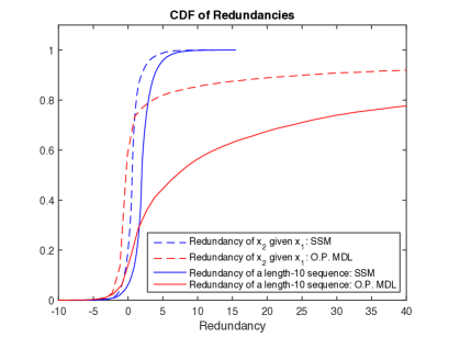
Figure 1: Redundancy comparison between ordinary predictive MDL (O.P. MDL) and our proposed sufficient statistic method for $\mu=0$ and $\sigma^{2}=4$.

V Scalar Signal Processing Methods

In the following we will derive MDL for various scalar signal processing methods. We can take inspiration from signal processing methods generally used for source coding, such as linear prediction and wavelets; however, the methods have to be modified for MDL, as we use lossless coding, not lossy coding. As often in signal processing, the models are a (deterministic) signal in Gaussian noise. In previous paper we have also considered non-Gaussian models [21]. All proofs are in Appendices.

V-A Iid Gaussian Case

A natural extension of the examples considered in Section IV-D is $x_{n}\sim\mathcal{N}(\mu,\sigma^{2})$ with both $\mu$ and $\sigma^{2}$ unknown. Define $\hat{\mu}_{n}=\frac{1}{n}\sum_{i=1}^{n}x_{i}$ and $S_{n}^{2}=\frac{1}{n-1}\sum_{i=1}^{n}\left(x_{i}-\hat{\mu}_{n}\right)^{2}$. Then the sufficient statistic method is

$$f(x_{n+1}|x^{n}) =\sqrt{\frac{n}{\pi\left(n+1\right)}}\frac{\Gamma\left(\frac{n}{2}\right)}{\Gamma\left(\frac{n-1}{2}\right)}$$

$$\times\frac{\left[\left(n-1\right)S_{n}^{2}\right]^{\frac{n-1}{2}}}{\left[nS_{n+1}^{2}\right]^{\frac{n}{2}}}$$ (18)

This is a special case of the vector Gaussian model considered later, so we will not provide a proof.

V-A1 Linear Transformations

The iid Gaussian case is a fundamental building block for other MDL methods. The idea is to find a linear transformation so that we can model the result as iid, and then use the iid Gaussian MDL. For example, in the vector case, suppose $\mathbf{x}_{n}\sim N(\boldsymbol{\mu},\boldsymbol{\Sigma})$ is (temporally) iid, and let $\mathbf{y}_{n}=\mathbf{A}\mathbf{x}_{n}\sim N(\mathbf{A}\boldsymbol{\mu},\mathbf{A}\boldsymbol{\Sigma}\mathbf{A}^{T})$. If we then assume that $\mathbf{A}\boldsymbol{\Sigma}\mathbf{A}^{T}$ is diagonal, we can use the iid Gaussian MDL on each component. Similarly, in the scalar case, we can use a filter instead of a matrix. Because of (2) we need to require $\mathbf{A}$ to be orthonormal: for any input we then have $\mathbf{y}_{n}^{T}\mathbf{y}_{n}=\mathbf{x}_{n}^{T}\mathbf{A}^{T}\mathbf{A}\mathbf{x}_{n}=\mathbf{x}_{n}^{T}\mathbf{x}_{n}$, and in particular $E[\mathbf{y}_{n}^{T}\mathbf{y}_{n}]=E[\mathbf{x}_{n}^{T}\mathbf{x}_{n}]$ independent of the actual $\boldsymbol{\Sigma}$. We will see this approach in several cases in the following.

V-B Linear Prediction

Linear prediction is a fundamental to random processes. Write

$$\hat{x}_{n+1|x^{n}} =\overset{\infty}{\underset{k=0}{\sum}}w_{k}x_{n-k}$$

$$e_{n+1} =x_{n+1}-\hat{x}_{n+1|x^{n}}$$

Then for most stationary random processes the resulting random process $\{e_{n}\}$ is uncorrelated, and hence in the Gaussian case, iid, by the Wold decomposition [19]. It is therefore a widely used method for source coding, e.g., [5]. In practical coding, a finite prediction order $M$ is used,

$$\hat{x}_{n+1|x^{n}} =\overset{M}{\underset{k=1}{\sum}}w_{k}x_{n-k+1},\quad n\geq M$$

Denote by $\tau$ the power of $\{e_{n}\}$. Consider the simplest case with $M=1$: there are two unknown parameters $(w_{1},\tau)$. However, the minimal sufficient statistic has dimension three [22]: $\left(\sum_{k=1}^{n}x_{k}^{2},\sum_{k=1}^{n-1}x_{k}^{2},\sum_{k=2}^{n}x_{k}x_{k-1}\right)$. Therefore, we cannot use SSM; and even if we could, the distribution of the sufficient statistic is not known in closed form [22]. We therefore turn to the NLM.

We assume that $e_{n+1}=x_{n+1}-\hat{x}_{n+1|x^{n}}$ is iid normally distributed with zero mean and variance $\tau$,

$$f(x^{n}|\tau,\mathbf{w}) =\frac{1}{(2\pi\tau)^{(n-M)/2}}$$

$$\times\exp\left(-\frac{1}{2\tau}\sum_{i=M+1}^{n}\left[x_{i}-\sum_{k=1}^{M}w_{k}x_{i-k}\right]^{2}\right)$$ (19)

Define

$$\hat{r}_{(n)}(k) =\sum_{i=M+1}^{n}x_{i}x_{i-k}$$

Then a simple calculation shows that

$$\sum_{i=M+1}^{n}e_{i}^{2} =\hat{r}_{(n)}(0)-2\mathbf{w}^{T}\mathbf{p}_{(n)}+\mathbf{w}^{T}R_{(n)}^{(M)}\mathbf{w}$$

where $\mathbf{w}^{T}=[w_{1}\;w_{2}\;\cdots\;w_{M}]$, $\mathbf{p}_{(n)}^{T}=[\hat{r}_{(n)}(1)\;\hat{r}_{(n)}(2)\;\cdots\;\hat{r}_{(n)}(M)]$,

$$R_{(n)}^{(M)} =\sum_{i=M+1}^{n}\mathbf{x}_{i-M}^{i-1}\left(\mathbf{x}_{i-M}^{i-1}\right)^{T}$$ (20)

and $x_{i-M}^{i-1}=[x_{i-1},x_{i-2},\ldots,x_{i-M}]$. Thus

$$f(x^{n}|\tau,\mathbf{w}) =\frac{1}{(2\pi\tau)^{(n-M)/2}}$$

$$\times\exp\left(-\frac{1}{2\tau}\left[\hat{r}_{(n)}(0)-2\mathbf{w}^{T}\mathbf{p}_{(n)}+\mathbf{w}^{T}R_{(n)}^{(M)}\mathbf{w}\right]\right)$$

giving (see Appendix A)

$$C(x^{n}) =\frac{1}{2\left(\pi\right)^{\frac{n-2M}{2}}\sqrt{\det\left(R_{(n)}\right)}}\frac{\Gamma\left(\frac{n-2M-2}{2}\right)}{\left(\hat{\tau}_{(n)}^{(M)}\right)^{\frac{n-2M-2}{2}}}$$

and

$$f_{M}(x_{n+1}|x^{n}) =\sqrt{\frac{\det\left(R_{(n)}^{(M)}\right)}{\det\left(R_{(n+1)}^{(M)}\right)}}\frac{\Gamma\left(\frac{n-2M-1}{2}\right)}{\Gamma\left(\frac{n-2M-2}{2}\right)}$$

$$\times\frac{1}{\sqrt{\pi}}\frac{\left(\hat{\tau}_{(n)}^{(M)}\right)^{\frac{n-2M-2}{2}}}{\left(\hat{\tau}_{(n+1)}^{(M)}\right)^{\frac{n-2M-1}{2}}}$$ (21)

with $\hat{\tau}_{(n)}^{(M)}=\hat{r}_{(n)}(0)-\mathbf{\mathbf{p}}_{(n)}^{T}R_{(n)}^{-1}\mathbf{p}_{(n)}$.

The equation (21) is defined for $n\geq 2M+2$: the vector $x_{i-M}^{i-1}$ is defined for $i\geq M+1$, and $R_{(n)}^{(M)}$ defined by (20) becomes full rank when the sum contains $M$ terms. Before the order $M$ linear predictor becomes defined, the data needs to be encoded with other methods. Since in atypicality we are not seeking to determine the model of data, just if a different model than the typical is better, we encode data with lower order linear predictors until the order $M$ linear predictor becomes defined. So, the first sample is encoded with the default pdf. The second and third samples are encoded with the iid unknown variance coder (16). Then the order 1 linear predictor takes over, and so on.

V-C Filterbanks and Wavelets

A popular approach to source coding is subband coding and waveletts [23, 24, 25]. The basic idea is to divide the signal into (perhaps overlapping) spectral subbands and then allocate different bitrates to each subband; the bitrate can be dependent on the power in the subband and auditory properties of the ear in for example audio coding. In MDL we need to do lossless coding, so this approach cannot be directly applied, but we can still use subband coding as explained in the following.

As we are doing lossless coding, we will only consider perfect reconstruction filterbanks [26, 23]. Furthermore, in light of Section V-A1 we also consider only (normalized) orthogonal filterbanks [23, 25].

The basic idea is that we split the signal into a variable number of subbands by putting the signal through the filterbank and downsampling. Then the output of each downsampled filter is coded with the iid Gaussian coder of Section V-A with an unknown mean and variance specific to each subband. In order to understand how this works, consider a filterbank with two subbands. Assume that the signal is stationary zero mean Gaussian with power $\sigma^{2}$, and let the power at the output of subband 1 be $\sigma_{1}^{2}$ and of subband 2 be $\sigma_{2}^{2}$. Because the filterbank is orthogonal, we have $\sigma^{2}=\frac{1}{2}\left(\sigma_{1}^{2}+\sigma_{2}^{2}\right)$. For analysis purposes, using (4) it is straightforward to see that we get the approximate codelengths

$$L_{\text{direct}} =\frac{l}{2}\log\left(\sigma^{2}\right)+\frac{l}{2}\left(\log 2\pi+\log e\right)+\frac{1}{2}\log l$$

$$L_{\text{filterbank}} =\frac{l}{4}\log\left(\sigma_{1}^{2}\right)+\frac{l}{4}\left(\log 2\pi+\log e\right)+\frac{1}{2}\log l$$

$$+\frac{l}{4}\log\left(\sigma_{1}^{2}\right)+\frac{l}{4}\left(\log 2\pi+\log e\right)+\frac{1}{2}\log l$$

$$=\frac{l}{2}\log\left(\sqrt{\sigma_{1}^{2}\sigma_{2}^{2}}\right)+\frac{l}{2}\left(\log 2\pi+\log e\right)+\log l$$

Since $\sqrt{\sigma_{1}^{2}\sigma_{2}^{2}}\leq\sigma^{2}$ (with equality only if $\sigma_{1}^{2}=\sigma_{2}^{2}$), the subband coder will result in shorter codelength for sufficiently large $l$ if the signal is non-white.

The above analysis is a stationary analysis for long sequences. However, when considering shorter sequences, we also need to consider the transient. The main issue is that output power will deviate from the stationary value during the transient, and this will affect the estimated power $\widehat{\sigma_{n}^{2}}$ used in the sequential MDL. The solution is to transmit to the receiver the input to the filterbank during the transient, and only use the output of the filterbank once the filters have been filled up. It is easy to see that the system is still perfect reconstruction: Using the received input to the filterbank, the receiver puts this through the analysis filterbank. It now has the total sequence produced by the analysis filterbank, and it can then put that through the reconstruction filterhank. When using multilevel filterbanks, this has to be done at each level.

We assume the decoder knows which filters are used and the maximum depth $D$ used. In principle the encoder could now search over all trees of level at most $D$. The issue is that there are an astonishing large number of such trees; for example for $D=4$ there are 676 such trees. Instead of choosing the best, we can use the idea of the CTW [8, 27, 2] and weigh in each node: Suppose after passing a signal $x^{n}$ of an internal node $S$ through low-pass and high-pass filters and downsampler, $x_{L}^{n/2}$ and $x_{H}^{n/2}$ are produced in the children nodes of $S$. The weighted probability of $x^{n}$ in the internal node $S$ will be

$$f_{w}\left(x^{n}\right) =\frac{1}{2}f\left(x^{n}\right)+\frac{1}{2}f_{w}\left(x_{L}^{n/2}\right)f_{w}\left(x_{H}^{n/2}\right)$$

which is a good coding distribution for both a memoryless source and a source with memory [8, 27].

VI Vector Case

We now assume that a vector sequence $\mathbf{x}^{n}$, $\mathbf{x}_{i}\in\mathbb{R}^{M}$ is observed. The vector case allows for a more rich set of model and more interesting data discovery than the scalar case, for example atypical correlation between multiple sensors. It can also be applied to images [28], and to scalar data by dividing into blocks. That is in particular useful for the DFT, Section VI-D.

A specific concern is initialization. Applying sequential coding verbatim to the vector case means that the first vector $\mathbf{x}_{1}$ need to be encoded with the default coder, but this means the default coder influences codelength too much. Instead we suggest to encode the first vector as a scalar signal using the scalar Gaussian coder (unknown variance$\to$unknown mean/variance). That way only the first component of the first vector needs to be encoded with the default coder.

VI-A Vector Gaussian Case with Unknown $\boldsymbol{\mu}$

First assume $\boldsymbol{\mu}$ is unknown but $\Sigma$ is given. We define $\mathrm{etr}\left(\cdots\right)=\exp\left(\mathrm{trace}\left(\cdots\right)\right)$ and we have

$$f\left(\mathbf{x}^{n}|\boldsymbol{\mu}\right) =\frac{1}{\sqrt{\left(2\pi\right)^{kn}\det\left(\Sigma\right)^{n}}}$$

$$\times\exp\left\{-\frac{1}{2}\sum_{i=1}^{n}\left(\mathbf{x}_{i}-\boldsymbol{\mu}\right)^{T}\Sigma^{-1}\left(\mathbf{x}_{i}-\boldsymbol{\mu}\right)\right\}$$

We first consider the NLM. By defining $\hat{\boldsymbol{\mu}}_{n}=\frac{1}{n}\sum_{i=1}^{n}\mathbf{x}_{i}$ and $\hat{\Sigma}_{n}=\sum_{i=1}^{n}\mathbf{x}_{i}\mathbf{x}_{i}$ (note that $\hat{\Sigma}_{n}$ is not the estimate of $\Sigma$) we have

$$C\left(\mathbf{x}^{n}\right) =\int f\left(\mathbf{x}^{n}|\boldsymbol{\mu}\right)d\boldsymbol{\mu}$$

$$=\frac{1}{\sqrt{\left(2\pi\right)^{kn}\det\left(\Sigma\right)^{n}}}\exp\left\{-\frac{1}{2}\sum_{i=1}^{n}\mathbf{x}_{i}\Sigma^{-1}\mathbf{x}_{i}\right\}$$

$$\times\int\exp\left\{-\frac{n}{2}\boldsymbol{\mu}^{T}\Sigma^{-1}\boldsymbol{\mu}+n\hat{\boldsymbol{\mu}}_{n}^{T}\Sigma^{-1}\boldsymbol{\mu}\right\}d\boldsymbol{\mu}$$

$$=C\exp\left\{-\frac{1}{2}\sum_{i=1}^{n}\left(\mathbf{x}_{i}\Sigma^{-1}\mathbf{x}_{i}-\hat{\boldsymbol{\mu}}_{n}^{T}\Sigma^{-1}\hat{\boldsymbol{\mu}}_{n}\right)\right\}$$

$$=C\mathrm{etr}\left\{-\frac{1}{2}\left(\hat{\Sigma}_{n}-n\hat{\boldsymbol{\mu}}_{n}\hat{\boldsymbol{\mu}}_{n}^{T}\right)\Sigma^{-1}\right\}$$

where $C=\frac{1}{\sqrt{\left(2\pi\right)^{k\left(n-1\right)}n^{k}\det\left(\Sigma\right)^{n-1}}}$ hence we can write

$$f\left(\mathbf{x}_{n+1}|\mathbf{x}^{n}\right)=\frac{C\left(\mathbf{x}^{n+1}\right)}{C\left(\mathbf{x}^{n}\right)}$$

$$=\sqrt{\left(\frac{n}{n+1}\right)^{k}}\frac{1}{\sqrt{\left(2\pi\right)^{k}\det\left(\Sigma\right)}}$$

$$\times\frac{\mathrm{etr}\left\{-\frac{1}{2}\left(\hat{\Sigma}_{n+1}-\left(n+1\right)\hat{\boldsymbol{\mu}}_{n+1}\hat{\boldsymbol{\mu}}_{n+1}^{T}\right)\Sigma^{-1}\right\}}{\mathrm{etr}\left\{-\frac{1}{2}\left(\hat{\Sigma}_{n}-n\hat{\boldsymbol{\mu}}_{n}\hat{\boldsymbol{\mu}}_{n}^{T}\right)\Sigma^{-1}\right\}}$$ (22)

It turns out that in this case, the SSM gives the same result.

VI-B Vector Gaussian Case with Unknown $\Sigma$

Assume $\mathbf{x}_{n}\sim\mathcal{N}\left(\mathbf{0},\Sigma\right)$ where the covariance matrix is unknown

$$f\left(\mathbf{x}^{n}|\Sigma\right) =\frac{1}{\sqrt{\left(2\pi\right)^{kn}\det\left(\Sigma\right)^{n}}}\mathrm{etr}\left\{-\frac{1}{2}\hat{\Sigma}_{n}\Sigma^{-1}\right\}$$

where $\hat{\boldsymbol{\Sigma}}_{n}=\sum_{i=1}^{n}\mathbf{x}_{i}\mathbf{x}_{i}^{T}$.

In order to find the MDL using SSM, notice that we can write

$$\mathbf{x}_{n}=\mathbf{S}\mathbf{z}_{n},\quad\mathbf{z}_{n}\sim\mathcal{N}(0,\mathbf{I})$$

where $\mathbf{S}=\boldsymbol{\Sigma}^{\frac{1}{2}}$, that is $\mathbf{S}$ is some matrix that satisfies $\mathbf{S}\mathbf{S}^{T}=\boldsymbol{\Sigma}$. A sufficient statistic for $\boldsymbol{\Sigma}$ is

$$\hat{\boldsymbol{\Sigma}}_{n}=\sum_{i=1}^{n}\mathbf{x}_{i}\mathbf{x}_{i}^{T}=\mathbf{S}\sum_{i=1}^{n}\mathbf{z}_{i}\mathbf{z}_{i}^{T}\mathbf{S}^{T}\stackrel{{\scriptstyle\text{def}}}{{=}}\mathbf{S}\mathbf{U}\mathbf{S}^{T}$$

Let $\hat{\mathbf{S}}_{n}=\hat{\boldsymbol{\Sigma}}_{n}^{\frac{1}{2}}=\mathbf{S}\mathbf{U}^{\frac{1}{2}}$. Then we can solve $\mathbf{S}=\hat{\mathbf{S}}_{n}\mathbf{U}^{-\frac{1}{2}}$ and $\boldsymbol{\Sigma}=\mathbf{\hat{S}}_{n}\mathbf{U}^{-1}\mathbf{\hat{S}}_{n}^{T}$. Since $\mathbf{U}^{-1}$ has Inverse-Wishart distribution $\mathbf{U}^{-1}\sim\mathcal{W}_{M}^{-1}\left(I,n\right)$, one can write $\Sigma\sim\mathcal{W}_{M}^{-1}\left(\hat{\Sigma}_{n},n\right)$. Using this distribution we calculate in Appendix B that

$$f\left(\mathbf{x}_{n+1}|\mathbf{x}^{n}\right) =\frac{1}{\pi^{\frac{M}{2}}}\frac{\det\left(\hat{\Sigma}_{n}\right)^{\frac{n}{2}}}{\det\left(\hat{\Sigma}_{n+1}\right)^{\frac{n+1}{2}}}\frac{\Gamma_{M}\left(\frac{n+1}{2}\right)}{\Gamma_{M}\left(\frac{n}{2}\right)}$$ (23)

where $\Gamma_{M}$ is the multivariate gamma function [16].

On the other hand, using the normalized likelihood method we have

$$C\left(\mathbf{x}^{n}\right) =\frac{\Gamma_{M}\left(\frac{n}{2}-\frac{M+1}{2}\right)}{2^{\frac{M\left(M+1\right)}{2}}\pi^{\frac{kn}{2}}\det\left(\hat{\Sigma}_{n}\right)^{\frac{n}{2}-\frac{M+1}{2}}}$$

From which

$$f\left(\mathbf{x}_{n+1}|\mathbf{x}^{n}\right) =\frac{C\left(\mathbf{x}^{n+1}\right)}{C\left(\mathbf{x}^{n}\right)}$$

$$=\frac{1}{\pi^{\frac{k}{2}}}\frac{\det\left(\hat{\Sigma}_{n}\right)^{\frac{n}{2}-\frac{M+1}{2}}}{\det\left(\hat{\Sigma}_{n+1}\right)^{\frac{n}{2}-\frac{M}{2}}}\frac{\Gamma_{M}\left(\frac{n}{2}-\frac{M}{2}\right)}{\Gamma_{M}\left(\frac{n}{2}-\frac{M+1}{2}\right)}$$ (24)

VI-C Vector Gaussian Case with Unknown $\boldsymbol{\mu}$ and $\Sigma$

Assume $\mathbf{x}_{n}\sim\mathcal{N}\left(\boldsymbol{\mu},\Sigma\right)$ where both mean and covariance matrix are unknown

$$f\left(\mathbf{x}^{n}|\boldsymbol{\mu},\Sigma\right) =\frac{1}{\sqrt{\left(2\pi\right)^{Mn}\det\left(\Sigma\right)^{n}}}$$

$$\times\exp\left\{-\frac{1}{2}\sum_{i=1}^{n}\left(\mathbf{x}_{i}-\boldsymbol{\mu}\right)^{T}\Sigma^{-1}\left(\mathbf{x}_{i}-\boldsymbol{\mu}\right)\right\}$$

It is well-known [17] that sufficient statistics are $\hat{\boldsymbol{\mu}}_{n}=\frac{1}{n}\sum_{i=1}^{n}\mathbf{x}_{i}$ and $\hat{\boldsymbol{\Sigma}}_{n}=\left(n-1\right)S_{n}=\sum_{i=1}^{n}\left(\mathbf{x}_{i}-\hat{\boldsymbol{\mu}}_{n}\right)\left(\mathbf{x}_{i}-\hat{\boldsymbol{\mu}}_{n}\right)^{T}$. Let $\mathbf{S}$ be a square root of $\boldsymbol{\Sigma}$, i.e., $\mathbf{S}\mathbf{S}^{T}=\boldsymbol{\Sigma}$. We can then write

$$\hat{\boldsymbol{\mu}}_{n} =\boldsymbol{\mu}+\frac{1}{\sqrt{n}}\mathbf{S}\mathbf{z}$$

$$\hat{\boldsymbol{\Sigma}}_{n} =\mathbf{S}\mathbf{U}\mathbf{S}^{T}$$

where $\mathbf{z}\sim\mathcal{N}\left(\mathbf{0},I\right)$ and $\mathbf{U}\sim\mathcal{W}_{M}\left(\mathbf{I},n-1\right)$, $\mathbf{z}$ and $\mathbf{U}$ are independent, and $\mathcal{W}_{M}$ is the Wishart distribution. We solve the second equation with respect to $\mathbf{S}$ as in Section VI-B and the first with respect to $\boldsymbol{\mu}$, to get

$$\boldsymbol{\Sigma} =\hat{\mathbf{S}}_{n}\mathbf{U}^{-1}\hat{\mathbf{S}}_{n}^{T}\sim\mathcal{W}_{M}^{-1}\left(\hat{\boldsymbol{\Sigma}}_{n},n-1\right)$$

$$\boldsymbol{\mu} =\hat{\boldsymbol{\mu}}_{n}-\frac{1}{\sqrt{n}}\mathbf{S}\mathbf{z}=\hat{\boldsymbol{\mu}}_{n}-\frac{1}{\sqrt{n}}\hat{\mathbf{S}}_{n}\mathbf{U}^{-\frac{1}{2}}\mathbf{z}\sim\mathcal{N}\left(\hat{\boldsymbol{\mu}}_{n},\frac{1}{n}\Sigma\right)$$

where $\hat{\mathbf{S}}_{n}$ is a square root of $\hat{\boldsymbol{\Sigma}}_{n}$. We can explicitly write the distributions as

$$f_{\mathbf{x}^{n}}\left(\boldsymbol{\mu}|\Sigma\right) =\sqrt{\frac{n^{M}}{\left(2\pi\right)^{M}\det\left(\Sigma\right)}}\exp\left\{-\frac{n}{2}\left(\boldsymbol{\mu}-\hat{\boldsymbol{\mu}}_{n}\right)^{T}\Sigma^{-1}\left(\boldsymbol{\mu}-\hat{\boldsymbol{\mu}}_{n}\right)\right\}$$

$$f_{\mathbf{x}^{n}}\left(\Sigma\right) =\frac{\det\left(\hat{\Sigma}_{n}\right)^{\frac{n-1}{2}}}{2^{\frac{M\left(n-1\right)}{2}}\Gamma_{M}\left(\frac{n-1}{2}\right)}\det\left(\Sigma\right)^{-\frac{n+M}{2}}\mathrm{etr}\left\{-\frac{1}{2}\hat{\Sigma}_{n}\Sigma^{-1}\right\}$$

Using these distributions, in Appendix C we calculate

$$f\left(\mathbf{x}_{n+1}|\mathbf{x}^{n}\right) =\frac{1}{\pi^{\frac{M}{2}}}\sqrt{\left(\frac{n}{n+1}\right)^{M}}\frac{\det\left(\hat{\Sigma}_{n}\right)^{\frac{n-1}{2}}}{\det\left(\hat{\Sigma}_{n+1}\right)^{\frac{n}{2}}}\frac{\Gamma_{M}\left(\frac{n}{2}\right)}{\Gamma_{M}\left(\frac{n-1}{2}\right)}$$

and for NLM

$$f\left(\mathbf{x}_{n+1}|\mathbf{x}^{n}\right) =\frac{1}{\pi^{\frac{M}{2}}}\sqrt{\left(\frac{n}{n+1}\right)^{M}}\frac{\det\left(\hat{\Sigma}_{n}\right)^{\frac{n-1}{2}-\frac{M+1}{2}}}{\det\left(\hat{\Sigma}_{n+1}\right)^{\frac{n}{2}-\frac{M+1}{2}}}$$

$$\times\frac{\Gamma_{M}\left(\frac{n-M-1}{2}\right)}{\Gamma_{M}\left(\frac{n-M-2}{2}\right)}$$

These are very similar to the case of known mean, Section VI-B. We require one more sample before the distributions become well-defined, and $\boldsymbol{\Sigma}_{n}$ is defined differently.

VI-D Sparsity and DFT

We can specify a general method as follows. Let $\boldsymbol{\Phi}$ is an orthonormal basis of $\mathbb{R}^{M}$ and write the signal model as

$$\mathbf{x}_{n}=\sum_{i=1}^{N}(A_{i}+s_{i,n})\boldsymbol{\phi}_{j(i)}+\mathbf{w}_{n}$$

Here $N$ is the number of basis vectors used, and $j(i),i=1,\ldots,N$ their indices. The signal $s_{i,n}$ is iid $\mathcal{N}(0,\sigma_{i})$, the noise $\mathbf{w}_{n}$ iid $\mathcal{N}(0,\sigma^{2}\mathbf{I})$, and $A_{i},\sigma_{i}^{2},\sigma^{2}$ are unknown. If we let $\mathbf{y}_{n}=\boldsymbol{\Phi}^{T}\mathbf{x}_{n}$ and $J$ the indices of the signal components then

$$y_{j(i),n} =A_{i}+s_{i,n}+w_{j(i),n}=A_{i}+\tilde{s}_{i,n},\quad j(i)\in J$$

$$y_{j,n} =w_{j,n},\quad j\notin J$$

Thus the $y_{j(i),n}$ can be encoded with the scalar Gaussian encoder of Section V-A, while the $y_{j,n}$ can be encoded with a vector Gaussian encoder for $\mathcal{N}(0,\sigma^{2}\mathbf{I}_{M-N})$ using the following equation that is achieved using the SSM

$$f\left(\mathbf{w}_{n+1}|\mathbf{w}^{n}\right) =\frac{1}{\pi^{\frac{\left(M-N\right)}{2}}}\frac{\Gamma\left(\frac{\left(M-N\right)\left(n+1\right)}{2}\right)}{\Gamma\left(\frac{\left(M-N\right)n}{2}\right)}$$

$$\times\frac{\left[n\widehat{\tau}_{n}\right]^{\frac{\left(M-N\right)n}{2}}}{\left[\left(n+1\right)\widehat{\tau}_{n+1}\right]^{\frac{\left(M-N\right)\left(n+1\right)}{2}}}$$

where $\widehat{\tau}_{n}=\frac{1}{n}\sum_{i=1}^{n}\mathbf{w}_{i}^{T}\mathbf{w}_{i}$. Now we need to choose which coefficients $j(i)$ to choose as signal components and inform the decoder. The set $J$ can be communicated to the decoder by sending a sequence of $0,1$ encoded with the universal encoder of [4, Section 13.2] with $MH\left(\frac{N}{M}\right)+\frac{1}{2}\log M$ bits. The optimum set can in general only be found by trying all sets $J$ and choosing the one with shortest codelength, which is infeasible. A heuristic approach is to find the $N$ components with maximum power when calculated over the whole blocklength $l$. What still remains is how to choose $N$. It seems computationally feasible to start with $N=1$ and then increase $N$ by 1 until the codelength no longer decreases, since most of the calculations for $N$ can be reused for $N+1$.

We can apply this in particular when $\boldsymbol{\Phi}$ is a DFT matrix. In light of Section V-A1 we need to use the normalized form of the DFT. The complications is that output is complex, i.e., the $M$ real inputs result in $M$ complex outputs, or $2M$ real outputs. Therefore, care has to be taken with the symmetry properties of the output. Another option is to use DCT instead, which is well-developed and commonly used for compression.

VII Experimental Results

As an example of application of atypicality, we will consider transient detection [29]. In transient detection, a sensor records a signal that is pure noise most of the time, and the task is to find the sections of the signal that are not noise. In our terminology, the typical signal is noise, and the task is to find the atypical parts.

As data we used hydrophone recordings from a sensor in the Hawaiian waters outside Oahu, the Station ALOHA Cabled Observatory (“ACO”) [30]. The data used for this paper were collected (with sampling freuquency of 96 kHz which was then downsampled to 8 kHz) during a proof module phase of the project conducted between February 2007 and October 2008. The data was pre-processed by differentiation ($y[n]=x[n]-x[n-1])$ to remove a non-informative mean component.

The principal goal of this two years of data is to locate whale vocalization. Fin (22 meters, up to 80 tons) and sei (12-18 meters, up to 24.6 tons) whales are known by means of visual and acoustic surveys to be present in the Hawaiian Islands during winter and spring months, but migration patterns in Hawaii are poorly understood [30].

Ground truth has been established by manual detection, which is achieved using visual inspection of spectrogram by a human operator. 24 hours of manual detections for both the 20 Hz and the 20-35 Hz variable calls were recorded for each the following dates (randomly chosen): 01 March 2007, 17 November 2007, 29 May 2008, 22 August 2008, 04 September 2008 and 09 February 2008 [30].

In order to analyze the performance of different detectors on such a data, first the measures Precision and Recall are defined as below

Recall $$=\frac{\text{number\,of\,correct\,detection}s}{\text{total\,number\,of\,manual\,detections}}$$

Precision $$=\frac{\text{number\,of\,correct\,detections}}{\text{total\,number\,of\,algorithm\,detections}}$$

where Recall measures the probability of correctly obtained vocalizations over expected number of detections and Precision measures the probability of correctly detected vocalizations obtained by the detector. The Precision versus Recall curve show the detectors ability to obtain vocalizations as well as the accuracy of these detections [30].

In order to compare our atypicality method with alternative approaches in transient detection, we compare its performance with Variable Threshold Page (VTP) which outperforms other similar methods in detection of non-trivial signals [31].

For the atypicality approach, we need a typical and and an atypical coder. The typical signal is pure noise, which, however, is not necessarily white: it consists of background noise, wave motion, wind and rain. We therefore used a linear predictive coder. The order of the linear predictive coder was globally set to 10 as a compromise between performance and computational speed. An order above 10 showed no significant decrease in codelength, while increasing computation time. The prediction coefficients were estimated for each 5-minute segment of data. It seems unreasonable to expect the prediction coefficients to be globally constant due to for example variations in weather, but over short length segments they can be expected to be constant. Of course, a 5 minute segment could contain atypical data and that would result in incorrect typical prediction coefficients. However, for this particular data we know (or assume) that atypical segments are of very short duration, and therefore will affect the estimated coefficients very little. This cannot be used for general data sets, only for data sets where there is a prior knowledge (or assumption) that atypical data are rare and short. Otherwise the typical coder should be trained on data known to be typical as in [2] or by using unsupervised atypicality [32].

For the atypical coder, we implemented all the scalar methods of section V in addition to the DFT, Section VI-D, with optimization over blocklength. Searching for atypical sequence (in this case, whale vocalizations) was then performed in different stages (more details of algorithm implementation can be found in [14]). Fig. 2 shows Precision vs Recall curve for both atypicality and VTP.

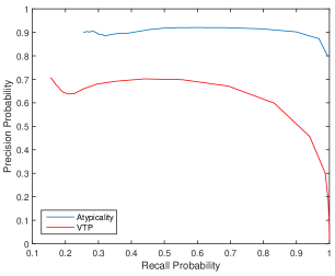
Figure 2: Precision vs Recall probability for all six days that manual detections are available

VIII Conclusion

Atypicality is a method for finding rare, interesting snippets in big data. It can be used for anomaly detection, data mining, transient detection, and knowledge extraction among other things. The current paper extended atypicality to real-valued data. It is important here to notice that discrete-valued and real-valued atypicality is one theory. Atypicality can therefore be used on data that are of mixed type. One advantage of atypicality is that it directly applies to sequences of variable length. Another advantage is that there is only one parameter that regulates atypicality, the single threshold parameter $\tau$, which has the concrete meaning of the logarithm of the frequency of atypical sequences. This contrasts with other methods that have multiple parameters.

Atypicality becomes really interesting in combination with machine learning. First, atypicality can be used to find what is not learned in machine learning. Second, for many data sets, machine learning is needed to find the typical coder. In the experiments in this paper, we did not need machine learning because the typical data was pure noise. But in many other types of data, e.g., ECG (electrocardiogram), “normal” data is highly complex, and the optimum coder has to be learned with machine learning. This is a topic for future research.

Appendix A Linear Prediction

we showed

$$f(x^{n}|\tau,\mathbf{w}) =\frac{1}{(2\pi\tau)^{(n-M)/2}}$$

$$\times\exp\left(-\frac{1}{2\tau}\left[\hat{r}_{(n)}(0)-2\mathbf{w}^{T}\mathbf{p}_{(n)}+\mathbf{w}^{T}R_{(n)}^{(M)}\mathbf{w}\right]\right)$$

therefore using NLM we have

$$C(x^{n}) =\int\int f(x^{n}|\tau,\mathbf{w})d\mathbf{w}d\tau$$

$$=A\int_{\tau}\tau^{-\frac{\left(n-M\right)}{2}}\exp\left\{-\frac{\hat{r}_{(n)}(0)}{2\tau}\right\}e_{1}\left(\tau\right)d\tau$$

where $A=\frac{1}{(2\pi)^{\left(n-M\right)/2}}$ and $e_{1}\left(\tau\right)=\int_{\mathbf{w}}\exp\left\{-\frac{1}{2\tau}\left[\mathbf{w}^{T}R_{(n)}\mathbf{w-}2\mathbf{p}_{(n)}^{T}\mathbf{w}\right]\right\}d\mathbf{w}$. Hence

$$C(\mathbf{x}^{n}) =B\int_{\tau}\tau^{-\frac{n-2M}{2}}\exp\left\{-\frac{1}{2\tau}\left[\hat{r}_{(n)}(0)-\mathbf{\mathbf{p}}_{(n)}^{T}R_{(n)}^{-1}\mathbf{p}_{(n)}\right]\right\}d\tau$$

$$=B\int_{\tau}\tau^{-\frac{n-2M}{2}}\exp\left\{-\frac{1}{2\tau}\hat{\tau}_{(n)}^{(M)}\right\}d\tau$$

$$=\frac{1}{2\left(\pi\right)^{\frac{n-2M}{2}}\sqrt{\det\left(R_{(n)}\right)}}\frac{\Gamma\left(\frac{n-2M-2}{2}\right)}{\left(\hat{\tau}_{(n)}^{(M)}\right)^{\frac{n-2M-2}{2}}}$$

where $B=\frac{1}{(2\pi)^{\left(n-2M\right)/2}\sqrt{\det\left(R_{(n)}\right)}}$.

Appendix B Vector Gaussian Case: unknown $\Sigma$

We showed that $\Sigma$ has Inverse-Wishart distribution $\Sigma\sim\mathcal{W}_{M}^{-1}\left(\hat{\Sigma}_{n},n\right)$ where $\hat{\Sigma}_{n}=\sum_{i=1}^{n}\mathbf{x}_{i}\mathbf{x}_{i}$ , hence

$$f_{\mathbf{x}^{n}}\left(\Sigma\right) =\frac{\det\left(\hat{\Sigma}_{n}\right)^{\frac{n}{2}}}{2^{\frac{nM}{2}}\Gamma_{M}\left(\frac{n}{2}\right)}\det\left(\Sigma\right)^{-\frac{n+M+1}{2}}\mathrm{etr}\left\{-\frac{1}{2}\hat{\Sigma}_{n}\Sigma^{-1}\right\}$$

and since

$$f\left(\mathbf{x}_{n+1}|\Sigma\right) =\frac{1}{\sqrt{\left(2\pi\right)^{M}\det\left(\Sigma\right)}}\mathrm{etr}\left\{-\frac{1}{2}\left(\hat{\Sigma}_{n+1}-\hat{\Sigma}_{n}\right)\Sigma^{-1}\right\}$$

therefore we have

$$f\left(\mathbf{x}_{n+1}|\mathbf{x}^{n}\right) =\int_{\Sigma>0}f\left(\mathbf{x}_{n+1}|\Sigma\right)f_{\mathbf{x}^{n}}\left(\Sigma\right)d\Sigma$$

$$=C\int_{\Sigma>0}\det\left(\Sigma\right)^{-\frac{n+M+2}{2}}\mathrm{etr}\left\{-\frac{1}{2}\hat{\Sigma}_{n+1}\Sigma^{-1}\right\}d\Sigma$$

$$\overset{(A)}{=}C\int_{Y>0}\det\left(Y\right)^{\frac{n}{2}-\frac{M}{2}}\mathrm{etr}\left\{-\frac{1}{2}\hat{\Sigma}_{n+1}Y\right\}dY$$

$$=D\int_{V>0}\det\left(V\right)^{\frac{n}{2}-\frac{M}{2}}\mathrm{etr}\left\{-V\right\}dV$$

$$\overset{(B)}{=}D\int_{V>0}\det\left(V\right)^{\frac{n+1}{2}-\frac{M+1}{2}}\mathrm{etr}\left\{-V\right\}dV$$

$$=\frac{1}{\pi^{\frac{M}{2}}}\frac{\det\left(\hat{\Sigma}_{n}\right)^{\frac{n}{2}}}{\det\left(\hat{\Sigma}_{n+1}\right)^{\frac{n+1}{2}}}\frac{\Gamma_{M}\left(\frac{n+1}{2}\right)}{\Gamma_{M}\left(\frac{n}{2}\right)}$$

where $C=\frac{\det\left(\hat{\Sigma}_{n}\right)^{\frac{n}{2}}}{2^{\frac{M\left(n+1\right)}{2}}\Gamma_{M}\left(\frac{n}{2}\right)\pi^{\frac{M}{2}}}$ and $D=\frac{\det\left(\hat{\Sigma}_{n}\right)^{\frac{n}{2}}}{\det\left(\hat{\Sigma}_{n+1}\right)^{\frac{n+1}{2}}}\frac{1}{\Gamma_{M}\left(\frac{n}{2}\right)\pi^{\frac{M}{2}}}$, and in equations (A) and (B) we changed the variable $\Sigma=Y^{-1}$ and $Y=2\hat{\Sigma}_{n}^{-\frac{1}{2}}V\hat{\Sigma}_{n}^{-\frac{1}{2}}$ respectively and $\Gamma_{m}\left(a\right)=\int_{V>0}\det\left(V\right)^{a-\frac{\left(m+1\right)}{2}}\mathrm{etr}\left\{-V\right\}dV$ is the multivariate Gamma function.

Appendix C Vector Gaussian Case: unknown $\boldsymbol{\mu}$ and $\Sigma$

We showed that $\boldsymbol{\mu}\sim\mathcal{N}\left(\hat{\boldsymbol{\mu}}_{n},\frac{1}{n}\Sigma\right)$ and $\Sigma\sim\mathcal{W}_{M}^{-1}\left(\hat{\Sigma}_{n},n-1\right)$ where $\hat{\boldsymbol{\mu}}_{n}=\frac{1}{n}\sum_{i=1}^{n}\mathbf{x}_{i}$ and $\hat{\boldsymbol{\Sigma}}_{n}=\sum_{i=1}^{n}\left(\mathbf{x}_{i}-\hat{\boldsymbol{\mu}}_{n}\right)\left(\mathbf{x}_{i}-\hat{\boldsymbol{\mu}}_{n}\right)^{T}$. Now using Bayes we can write the joint pdf as $f_{\mathbf{x}^{n}}\left(\boldsymbol{\mu},\Sigma\right)=f_{\mathbf{x}^{n}}\left(\boldsymbol{\mu}|\Sigma\right)f_{\mathbf{x}^{n}}\left(\Sigma\right)$. Define $A\stackrel{{\scriptstyle\text{def}}}{{=}}f\left(\mathbf{x}_{n+1}|\mathbf{x}^{n}\right)=\int_{\Sigma>0}\int f\left(\mathbf{x}_{n+1}|\boldsymbol{\mu},\Sigma\right)f_{\mathbf{x}^{n}}\left(\boldsymbol{\mu},\Sigma\right)d\boldsymbol{\mu}d\Sigma$

$$A =B\int_{\Sigma>0}\det\left(\Sigma\right)^{-\frac{n+M+2}{2}}e_{1}\left(\Sigma\right)e_{2}\left(\Sigma\right)d\Sigma$$

where

$$e_{1}\left(\Sigma\right) =\mathrm{etr}\left\{-\frac{1}{2}\left(\hat{\Sigma}_{n}+n\hat{\boldsymbol{\mu}}_{n}\hat{\boldsymbol{\mu}}_{n}^{T}+\mathbf{x}_{n+1}\mathbf{x}_{n+1}^{T}\right)\Sigma^{-1}\right\}$$

$$e_{2}\left(\Sigma\right) =\int\exp\left\{-\frac{n+1}{2}\left[\boldsymbol{\mu}^{T}\Sigma^{-1}\boldsymbol{\mu}-2\hat{\boldsymbol{\mu}}_{n+1}\Sigma^{-1}\boldsymbol{\mu}\right]\right\}d\boldsymbol{\mu}$$

$$=\sqrt{\frac{\left(2\pi\right)^{M}\det\left(\Sigma\right)}{\left(n+1\right)^{M}}}\exp\left\{\frac{n+1}{2}\hat{\boldsymbol{\mu}}_{n+1}^{T}\Sigma^{-1}\hat{\boldsymbol{\mu}}_{n+1}\right\}$$

$$B =\frac{\det\left(\hat{\Sigma}_{n}\right)^{\frac{n-1}{2}}}{\Gamma_{M}\left(\frac{n-1}{2}\right)}\frac{n^{\frac{M}{2}}}{2^{\frac{M\left(n-1\right)}{2}}\left(2\pi\right)^{M}}$$

now since $\hat{\Sigma}_{n+1}=\hat{\Sigma}_{n}+n\hat{\boldsymbol{\mu}}_{n}\hat{\boldsymbol{\mu}}_{n}^{T}+\mathbf{x}_{n+1}\mathbf{x}_{n+1}^{T}-\left(n+1\right)\hat{\boldsymbol{\mu}}_{n+1}\hat{\boldsymbol{\mu}}_{n+1}^{T}$, by defining $C\stackrel{{\scriptstyle\text{def}}}{{=}}B\sqrt{\frac{\left(2\pi\right)^{M}}{\left(n+1\right)^{M}}}=\sqrt{\left(\frac{n}{n+1}\right)^{M}}\frac{\det\left(\hat{\Sigma}_{n}\right)^{\frac{n-1}{2}}}{\Gamma_{M}\left(\frac{n-1}{2}\right)}\frac{1}{2^{\frac{M\left(n-1\right)}{2}}\left(2\pi\right)^{\frac{M}{2}}}$ we can write

$$A =C\int_{\Sigma>0}\det\left(\Sigma\right)^{-\frac{n+M+1}{2}}\mathrm{etr}\left\{-\frac{1}{2}\hat{\Sigma}_{n+1}\Sigma^{-1}\right\}d\Sigma$$

$$=C\int_{Y>0}\det\left(Y\right)^{\frac{n}{2}-\frac{M+1}{2}}\mathrm{etr}\left\{-\frac{1}{2}\hat{\Sigma}_{n+1}Y\right\}dY$$

$$=C\frac{2^{\frac{Mn}{2}}}{\det\left(\hat{\Sigma}_{n+1}\right)^{\frac{n}{2}}}\int_{V>0}\det\left(V\right)^{\frac{n}{2}-\frac{M+1}{2}}\mathrm{etr}\left\{-V\right\}dV$$

$$=\frac{1}{\pi^{\frac{M}{2}}}\sqrt{\left(\frac{n}{n+1}\right)^{M}}\frac{\det\left(\hat{\Sigma}_{n}\right)^{\frac{n-1}{2}}}{\det\left(\hat{\Sigma}_{n+1}\right)^{\frac{n}{2}}}\frac{\Gamma_{M}\left(\frac{n}{2}\right)}{\Gamma_{M}\left(\frac{n-1}{2}\right)}$$

References

- [1] V. Chandola, A. Banerjee, and V. Kumar, “Anomaly detection for discrete sequences: A survey,” Knowledge and Data Engineering, IEEE Transactions on, vol. 24, no. 5, pp. 823 –839, may 2012.
- [2] A. Høst-Madsen, E. Sabeti, and C. Walton, “Data discovery and anomaly detection using atypicality,” IEEE Transactions on Information Theory, submitted, available at http://tinyurl.com/jndmvo7.
- [3] M. Li and P. Vitányi, An Introduction to Kolmogorov Complexity and Its Applications, 3rd ed. Springer, 2008.
- [4] T. Cover and J. Thomas, Information Theory, 2nd Edition. John Wiley, 2006.
- [5] F. Ghido and I. Tabus, “Sparse modeling for lossless audio compression,” Audio, Speech, and Language Processing, IEEE Transactions on, vol. 21, no. 1, pp. 14–28, Jan 2013.
- [6] J. Rissanen, “A universal prior for integers and estimation by minimum description length,” The Annals of Statistics, no. 2, pp. 416–431, 1983.
- [7] V. Kostina, “Data compression with low distortion and finite blocklength,” IEEE Transactions on Information Theory, vol. 63, no. 7, pp. 4268–4285, July 2017.
- [8] F. M. J. Willems, Y. Shtarkov, and T. Tjalkens, “The context-tree weighting method: basic properties,” Information Theory, IEEE Transactions on, vol. 41, no. 3, pp. 653–664, 1995.
- [9] P. D. Gr unwald, The Minimum Description Length Principle. MIT Press, 2007.
- [10] J. Rissanen, “Stochastic complexity and modeling,” The Annals of Statistics, no. 3, pp. 1080–1100, Sep. 1986.
- [11] R. J. Larsen and M. L. Marx, An introduction to mathematical statistics and its applications, 1986.
- [12] T. Roos and J. Rissanen, “On sequentially normalized maximum likelihood models,” in Workshop on Information Theoretic Methods in Science and Engineering (WITMSE-08), 2008.
- [13] P. Elias, “Universal codeword sets and representations of the integers,” Information Theory, IEEE Transactions on, vol. 21, no. 2, pp. 194 – 203, mar 1975.
- [14] A. Høst-Madsen and E. Sabeti, “Atypical information theory for real-valued data,” in Proceedings of International Symposium on Information Theory, 2015.
- [15] S. Verdú, Multiuser Detection. Cambridge, UK: Cambridge University Press, 1998.
- [16] R. J. Muirhead, Aspects of multivariate statistical theory. John Wiley & Sons, 2009, vol. 197.
- [17] L. L. Scharf, Statistical Signal Processing: Detection, Estimation, and Time Series Analysis. Addison-Wesley, 1990.
- [18] J. Rissanen, Stochastic complexity in statistical inquiry. World scientific, 1998, vol. 15.
- [19] G. R. Grimmett and D. R. Stirzaker, Probability and Random Processes, Third Edition. Oxford University Press, 2001.
- [20] E. Sabeti and A. Host-Madsen, “Enhanced mdl with application to atypicality,” in 2017 IEEE International Symposium on Information Theory (ISIT). IEEE, 2017.
- [21] E. Sabeti and A. Høst-Madsen, “Atypicality for the class of exponential family,” in 54th Annual Allerton Conference, Urbana-Champaign, Illinois, 2016.
- [22] G. Forchini, “The density of the sufficient statistics for a gaussian ar(1) model in terms of generalized functions,” Statistics & Probability Letters, vol. 50, no. 3, pp. 237 – 243, 2000. [Online]. Available: http://www.sciencedirect.com/science/article/pii/S0167715200001115
- [23] S. Mallat, A wavelet tour of signal processing: the sparse way. Academic press, 2008.
- [24] M. Vetterli and J. Kovacevic, Wavelets and Subband Coding. http://waveletsandsubbandcoding.org, 1995.
- [25] M. Vetterli and C. Herley, “Wavelets and filter banks: theory and design,” IEEE Transactions on Signal Processing, vol. 40, no. 9, pp. 2207–2232, Sep 1992.
- [26] S. K. Mitra and Y. Kuo, Digital signal processing: a computer-based approach. McGraw-Hill New York, 2006, vol. 2.
- [27] F. Willems, Y. Shtarkov, and T. Tjalkens, “Reflections on "the context tree weighting method: Basic properties",” Newsletter of the IEEE Information Theory Society, vol. 47, no. 1, 1997.
- [28] E. Sabeti and A. Høst-Madsen, “How interesting images are: An atypicality approach for social networks,” in 2016 IEEE International Conference on Big Data (Big Data 2016) Washington D.C, 2016.
- [29] C. Han, P. Willett, B. Chen, and D. Abraham, “A detection optimal min-max test for transient signals,” Information Theory, IEEE Transactions on, vol. 44, no. 2, pp. 866 –869, mar 1998.
- [30] K. Silver, “A passive acoustic automated detector for sei and fin whale calls,” Master’s thesis, University of Hawaii, 2014.
- [31] Z. J. Wang and P. Willett, “A variable threshold page procedure for detection of transient signals,” IEEE transactions on signal processing, vol. 53, no. 11, pp. 4397–4402, 2005.
- [32] E. Sabeti and A. Host-Madsen, “Universal data discovery using atypicality: Algorithms,” in 2017 IEEE International Conference on Big Data (Big Data 2017) Boston, MA, Submitted 2017.