Applying ACO To Large Scale TSP Instances

Abstract

Ant Colony Optimisation (ACO) is a well known metaheuristic that has proven successful at solving Travelling Salesman Problems (TSP). However, ACO suffers from two issues; the first is that the technique has significant memory requirements for storing pheromone levels on edges between cities and second, the iterative probabilistic nature of choosing which city to visit next at every step is computationally expensive. This restricts ACO from solving larger TSP instances. This paper will present a methodology for deploying ACO on larger TSP instances by removing the high memory requirements, exploiting parallel CPU hardware and introducing a significant efficiency saving measure. The approach results in greater accuracy and speed. This enables the proposed ACO approach to tackle TSP instances of up to 200K cities within reasonable timescales using a single CPU. Speedups of as much as 1200 fold are achieved by the technique.

1 Introduction

Ant Colony Optimisation (ACO) [8] is a metaheuristic which has demonstrated significant success in solving Travelling Salesman Problems (TSP) [7]. The technique simulates ants moving through a fully connected network using pheromone levels to guide their choices of which cities to visit next to build a complete tour. However, ACO has two drawbacks the first being significant memory requirements to store the pheromone levels on every edge. Secondly, simulating ants by making probabilistic decisions at each city to determine the next city to visit makes ACO computationally intensive. Therefore, ACO will struggle when applied to larger TSP instances. Consider, the pheromone matrix which requires an $n$ by $n$ matrix whereby $n$ is the number of cities. As the number of cities increases linearly, a quadratic increase in memory requirements is observed. The same is true for probabilistically simulating ants to construct a tour. This paper will address these issues enabling ACO to be applied to larger TSP instances.

The paper is laid out as follows; Section 2 will describe ACO, Section 3 will present a scalable version of ACO to apply to large scale TSP instances whilst Section 4 will demonstrate its effectiveness on well known TSP instances. Finally Section 5 demonstrates the approach on TSP instances of up to 200,000 cities.

2 ACO Applied to the TSP

The Travelling Salesman Problem (TSP) is a task where the objective is to visit every city in the problem once minimising the total distance travelled. The symmetric TSP can be represented as a complete weighted graph $G=(V,E,d)$ where $V=\{1,2,..,n\}$ is a set of vertices defining each city and $E=\{(i,j)|(i,j)\in V\times V\}$ the edges consisting of the distance $d$ between pairs of cities such that $d_{ij}=d_{ji}$. The objective is to find a Hamiltonian cycle in $G$ of minimal length.

Ant Colony Optimisation (ACO) applied to the TSP involves simulated ants moving through the graph $G$ visiting each city once and depositing pheromone as they go. The level of pheromone deposited is defined by the quality of the tour the given ant finds. Ants probabilistically decide which city to visit next using this pheromone level on the edges of graph $G$ and heuristic information based upon the distance between an ant’s current city and unvisited cities. An evaporation effect is used to prevent pheromone levels reaching a state of local optima. Therefore, ACO consists of two stages, the first tour construction and the second stage pheromone update. The tour construction stage involves $m$ ants constructing complete tours. Ants start at a random city and iteratively make probabilistic choices as to which city to visit next using the random proportional rule whereby the probability of ant $k$ at city $i$ visiting city $j\in N^{k}$ is defined as:

$$p_{ij}^{k}=\frac{[\tau_{ij}]^{\alpha}[\eta_{ij}]^{\beta}}{\sum_{l\in N^{k}}[\tau_{il}]^{\alpha}[\eta_{il}]^{\beta}}$$ (1)

where $[\tau_{il}]$ is the pheromone level deposited on the edge leading from city $i$ to city $l$; $[\eta_{il}]$ is the heuristic information consisting of the distance between city $i$ and city $l$ set at $1/d_{il}$; $\alpha$ and $\beta$ are tuning parameters controlling the relative influence of the pheromone deposit $[\tau_{il}]$ and the heuristic information $[\eta_{il}]$.

Once all ants have completed the tour construction stage, pheromone levels on the edges of graph $G$ are updated. First, evaporation of pheromone levels upon every edge of graph $G$ occurs whereby the level is reduced by a value $\rho$ relative to the pheromone upon that edge:

$$\tau_{ij}\leftarrow(1-\rho)\tau_{ij}$$ (2)

where $p$ is the evaporation rate typically set between 0 and 1. Once this evaporation is completed each ant $k$ will then deposit pheromone on the edges it has traversed based on the quality of the tour it found:

$$\tau_{ij}\leftarrow\tau_{ij}+\sum_{k=1}^{m}\Delta\tau_{ij}^{k}$$ (3)

where the amount of pheromone ant k deposits, $\Delta\tau_{ij}^{k}$ is defined by:

$$\Delta\tau_{ij}^{k} = \left\{\begin{array}[]{ll}1/C^{k},&\mbox{if edge $(i,j)$ belongs to $T^{k}$}\\ 0,&\mbox{otherwise}\\ \end{array}\right.$$ (6)

where $1/C^{k}$ is the length of ant $k$’s tour $T^{k}$. This methodology ensures that shorter tours found by an ant result in greater levels of pheromone being deposited on the edge of the given tour.

3 Addressing the Scalability of ACO

A key issue with ACO is its memory requirements in the form of the pheromone matrix which stores the the level of pheromone on every edge between each city. Thus an $n$ by $n$ size matrix is required in memory to store this information so for a 100,000 city problem, a 100,000 by 100,000 matrix is required. Using a float datatype requiring four bytes of memory, this matrix will need approximately 37 GB of memory, much more than typically available on CPUs. However, a variant of ACO exists which dispenses with the need for a pheromone matrix, Population-based ACO (P-ACO) [10]. With this approach, a population of tours are maintained ($k_{long}(t)$) whereby the best tour at each iteration $t$ is added. Since $k_{long}(t)$ is of a fixed size tours are added in a First In First Out (FIFO) manner. Pheromone levels are calculated by using the $k_{long}(t)$ information. An ant at a given city calculates the pheromone levels by examining the edges that were traversed in $k_{long}(t)$ from the given city. Thus there is no pheromone matrix and no pheromone evaporation. If $k_{long}(t)$ is significantly less than the number of cities then this is a considerable saving in memory requirements.

In this paper, some modifications to P-ACO are implemented. Firstly, instead of using a store of best found tours updated in a FIFO manner, each ant has a local memory ($l_{best}$) containing the best tour that the ant has found, a steady-state mechanism. These $l_{best}$ tours are used to provide pheromone level information to ants when probabilistically deciding which city to next visit. This is similar in effect to Particle Swarm Optimisation (PSO) [9] whereby particles use both their local best solution and a global best to update their position. Secondly, the amount of pheromone an edge from an $l_{best}$ tour contributes equates to the quality of the global best ($g_{best}$) tour divided by that of the $l_{best}$ hence a value between 0.0 and 1.0. These measures are taken to increase diversity.

Moreover, to gain the maximum available performance of the P-ACO approach from a CPU, an asynchronous parallel approach is used with multiple threads of execution and each thread simulates a number of ants. Moreover, the choosing of the next city to visit is decided by multiplying the heuristic information, the pheromone level and a random probabilistic value between 0.0 and 1.0 and the city with the greatest combined value is selected as the next to visit. This approach is known as the Independent Roulette approach [3]. This allows the utilisation of the extended Single Instruction Multiple Data (SIMD) registers available in a CPU through AVX for the probabilistic decision making process. These extra wide registers enable up to eight edge comparisons to be made in parallel. Using a parallel methodology with AVX registers improves the computational speed by approximately 30-40x when using a quad core processor.

3.1 Introducing PartialACO

The most computationally expensive aspect of the ACO algorithm is the tour construction phase. This aspect of ACO has an exponential increase in computation time cost as the number of cities increases. Moreover, as an ant repeatedly probabilistically decides at each city which to visit next it could be considered that the greater number of cities in a tour that requires constructing, the greater the probability an ant will eventually make a poor choice of city to visit next resulting in a low quality tour. Hence, it is hypothesised that perhaps it would be advantageous for ants to only change part of a known good tour. To do so would firstly reduce the computational complexity and secondly reduce the probability of an ant making a poor decision at some point of the tour construction. For the P-ACO approach detailed previously, the part of the tour that is not changed by an ant could be based upon its $l_{best}$ tour. Essentially, at each iteration an ant randomly chooses a city to start its tour from and then a random number of cities to preserve from its $l_{best}$ tour. The remaining part of the tour will be constructed as normal. This methodology is similar to crossover in Genetic Algorithms (GA) [11] for the TSP whereby a large section of a tour is preserved and the remaining aspect constructed from another tour whilst avoiding repetition. Figure 1 visualises the concept whereby the dark part of the $l_{best}$ tour is preserved and the rest discarded and then this partial tour is completed using ACO. Henceforth, this implementation of ACO will be referred to as PartialACO. A high level overview of the technique is shown in Algorithm 1.

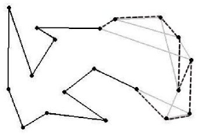
Figure 1: Illustration of PartialACO whereby the $l_{best}$ tour of an ant is partially modified by the ant. The dark part of the tour is retained and the lighter part discarded. PartialACO then completes the tour as normal creating a new tour (dashed line).

Algorithm 1 PartialACO

1:  for each ant do

2:     Generate initial tour using P-ACO approach

3:  end for

4:  for number of iterations do

5:     for each ant do

6:        Select random starting city from current $l_{best}$ tour

7:        Select random number of cities in $l_{best}$ tour to preserve

8:        Copy $l_{best}$ tour from starting city for the specified random number of cities

9:        Complete remaining aspect of tour using P-ACO approach

10:        If new tour better than $l_{best}$ tour then update $l_{best}$ tour

11:     end for

12:  end for

13:  Output best $l_{best}$ tour (the $g_{best}$ tour)

4 Experiments With PartialACO

To test the effectiveness of the PartialACO approach experiments will be conducted using five standard TSP problems of increasing size from the TSPLIB library. Sixteen ants, two per parallel thread of execution, will be simulated for 100,000 iterations with the $\alpha$ and $\beta$ parameters both set to a value of 5.0 to reduce the influence of heuristic information and increase the influence of pheromone from good tours. Results are averaged over 100 random runs and experiments are conducted using an Intel i7 processor using eight parallel threads of execution and the AVX registers. Table 1 shows the results from the standard P-ACO approach whereby full length tours are constructed by each ant at every iteration. The average accuracy ranges from between 4 and 13% of the known optimum. Table 2 demonstrates the results from the PartialACO approach described in this paper whereby only a portion of each ant’s best found tour is exposed to modification. From these results it can be observed that accuracy has been improved for all TSP instances by several percent. More importantly, the computational speed of the approach has been increased significantly. A speedup of up to 2.8x is observed with speedups increasing with the size of the TSP instance. Thus, PartialACO is demonstratively both faster and more accurate.

Table 1: Results from using standard P-ACO approach with accuracy expressed as percentage difference from known optimum. Results averaged over 100 random runs.

TSP Instance	Accuracy (% Error)			Execution Time (in seconds)
	Average	Best	Worst
pcb442	$4.16$ p m 1.37	$1.58$	$8.78$	$40.53$ p m 0.42
d657	$8.02$ p m 2.41	$3.43$	$12.44$	$72.87$ p m 0.53
rat783	$4.08$ p m 1.13	$2.27$	$7.82$	$96.23$ p m 0.81
pr1002	$7.88$ p m 1.49	$5.18$	$12.47$	$145.59$ p m 0.91
pr2392	$13.47$ p m 1.13	$10.91$	$15.98$	$688.13$ p m 2.86

Table 2: Results from using PartialACO approach with accuracy expressed as percentage difference from known optimum and relative speedup to using standard P-ACO approach. Results averaged over 100 random runs.

TSP Instance	Accuracy (% Error)			Execution Time (in seconds)	Relative Speedup
	Average	Best	Worst
pcb442	$2.72$ p m 0.67	$1.14$	$4.75$	$17.94$ p m 0.26	2.26x
d657	$4.33$ p m 0.73	$2.88$	$7.17$	$31.68$ p m 0.31	2.30x
rat783	$3.64$ p m 0.60	$2.18$	$5.99$	$40.01$ p m 0.40	2.41x
pr1002	$4.06$ p m 0.57	$2.61$	$5.24$	$58.27$ p m 0.33	2.50x
pr2392	$9.47$ p m 2.09	$5.01$	$12.84$	$245.96$ p m 0.88	2.80x

Table 3: Results from using PartialACO approach with restrictions on the maximum permissable modification. Accuracy expressed as percentage difference from known optimum with relative speedup to using standard P-ACO approach reported. Results are averaged over 100 random runs.

TSP Instance	Max. Modification	Accuracy (% Error)			Execution Time (in seconds)	Relative Speedup
		Average	Best	Worst
	50%	$4.90$ p m 1.31	$2.31$	$9.48$	$9.01$ p m 0.22	4.50x
	40%	$6.79$ p m 1.57	$3.64$	$10.11$	$7.44$ p m 0.18	5.45x
pcb442	30%	$8.95$ p m 1.71	$5.05$	$13.13$	$6.05$ p m 0.12	6.70x
	20%	$11.91$ p m 2.09	$6.36$	$15.52$	$4.91$ p m 0.10	8.26x
	10%	$16.59$ p m 2.16	$9.70$	$21.71$	$3.97$ p m 0.05	10.22x
	50%	$7.29$ p m 1.00	$5.14$	$9.66$	$14.48$ p m 0.22	5.03x
	40%	$8.40$ p m 1.34	$5.34$	$11.30$	$11.62$ p m 0.15	6.27x
d657	30%	$10.23$ p m 1.46	$6.84$	$13.87$	$9.27$ p m 0.16	7.86x
	20%	$13.12$ p m 1.97	$6.99$	$17.87$	$7.16$ p m 0.11	10.17x
	10%	$17.12$ p m 1.69	$12.21$	$22.37$	$5.53$ p m 0.06	13.17x
	50%	$7.67$ p m 1.38	$3.52$	$11.03$	$17.66$ p m 0.16	5.45x
	40%	$9.62$ p m 1.20	$4.73$	$12.41$	$14.08$ p m 0.15	6.83x
rat783	30%	$11.34$ p m 1.43	$7.46$	$15.95$	$10.91$ p m 0.18	8.82x
	20%	$13.46$ p m 1.68	$9.45$	$16.77$	$8.27$ p m 0.13	11.64x
	10%	$17.09$ p m 1.53	$11.78$	$20.97$	$5.98$ p m 0.08	16.10x
	50%	$7.10$ p m 1.32	$4.24$	$11.54$	$24.36$ p m 0.35	5.98x
	40%	$9.24$ p m 1.47	$5.73$	$13.03$	$19.34$ p m 0.27	7.53x
pr1002	30%	$10.52$ p m 1.70	$6.12$	$13.41$	$14.70$ p m 0.19	9.91x
	20%	$12.75$ p m 1.84	$7.96$	$16.98$	$10.93$ p m 0.16	13.33x
	10%	$16.32$ p m 1.57	$11.43$	$20.44$	$7.83$ p m 0.12	18.61x
	50%	$13.98$ p m 1.45	$11.41$	$16.61$	$82.76$ p m 0.37	8.31x
	40%	$16.37$ p m 1.18	$13.32$	$18.97$	$61.25$ p m 0.30	11.23x
pr2392	30%	$18.01$ p m 1.54	$14.15$	$21.14$	$43.45$ p m 0.17	15.84x
	20%	$20.01$ p m 1.56	$15.33$	$22.22$	$29.84$ p m 0.17	23.06x
	10%	$21.92$ p m 1.02	$19.87$	$24.56$	$20.74$ p m 0.18	33.18x

Although the initial results from PartialACO have demonstrated a speed advantage with improved accuracy, it is possible to increase the speed of the approach further. Currently, a random part of the local best tour of an ant is preserved and the rest exposed to ACO to modify it. However, the part that is modified could be restricted to a maximum percentage of the $l_{best}$ tour. For instance, a maximum percentage modification of 50% could be used thus for a 100 city problem at least part of the $l_{best}$ tour consisting of 50 cities will be preserved. Reducing the degree to which the $l_{best}$ tour of an ant can be changed could also improve tour quality by increased tour exploitation whilst also increasing the speed advantage of PartialACO. Table 3 demonstrates the results from restricting the maximum amount that an ant’s $l_{best}$ tour can be modified whereby it can be observed that by reducing the part of the $l_{best}$ tour that can be modified, the average accuracy deteriorates with respect to the known optimum. A potential reason for this is that the ants become trapped in local optima, unable to improve their $l_{best}$ tour without a greater degree of flexibility in tour construction. However, as expected, reducing the degree to which a $l_{best}$ tour can be modified increases the speed of the approach with up to a 33 fold increase in speed observed when only allowing a maximum 10% of $l_{best}$ tours to be modified at each iteration.

Table 4: Results from using PartialACO approach with 0.95 probability and restrictions on the maximum permissable modification. Accuracy expressed as percentage difference from known optimum with relative speedup to using standard P-ACO approach reported. Results are averaged over 100 random runs.

TSP Instance	Max. Modification	Accuracy (% Error)			Execution Time (in seconds)	Relative Speedup
		Average	Best	Worst
	50%	$2.55$ p m 0.94	$1.19$	$5.25$	$10.47$ p m 0.21	3.87x
	40%	$2.61$ p m 0.94	$1.01$	$5.22$	$9.00$ p m 0.22	4.50x
pcb442	30%	$3.26$ p m 1.41	$1.26$	$7.15$	$7.63$ p m 0.16	5.31x
	20%	$3.35$ p m 1.34	$1.43$	$7.95$	$6.37$ p m 0.13	6.36x
	10%	$3.96$ p m 1.67	$1.55$	$8.98$	$5.28$ p m 0.11	7.67x
	50%	$4.79$ p m 1.25	$2.61$	$7.71$	$17.08$ p m 0.21	4.27x
	40%	$5.28$ p m 1.26	$2.83$	$8.99$	$14.26$ p m 0.22	5.11x
d657	30%	$5.65$ p m 1.33	$2.95$	$9.03$	$12.05$ p m 0.20	6.05x
	20%	$6.34$ p m 1.39	$3.19$	$9.30$	$9.95$ p m 0.17	7.32x
	10%	$7.27$ p m 1.64	$3.38$	$11.39$	$8.15$ p m 0.13	8.94x
	50%	$4.46$ p m 1.45	$1.81$	$8.60$	$21.23$ p m 0.29	4.53x
	40%	$5.04$ p m 1.30	$2.37$	$7.53$	$17.92$ p m 0.22	5.37x
rat783	30%	$5.89$ p m 1.48	$2.25$	$9.40$	$14.91$ p m 0.20	6.45x
	20%	$6.99$ p m 1.30	$3.10$	$10.26$	$12.27$ p m 0.14	7.84x
	10%	$8.14$ p m 1.83	$3.30$	$10.90$	$9.95$ p m 0.16	9.67x
	50%	$4.75$ p m 1.33	$2.28$	$8.43$	$30.05$ p m 0.30	4.84x
	40%	$5.28$ p m 1.16	$2.91$	$7.97$	$24.96$ p m 0.28	5.83x
pr1002	30%	$6.02$ p m 1.23	$3.27$	$9.41$	$20.66$ p m 0.22	7.05x
	20%	$6.58$ p m 1.17	$3.69$	$9.04$	$16.95$ p m 0.21	8.59x
	10%	$8.11$ p m 1.46	$2.76$	$10.55$	$13.88$ p m 0.15	10.49x
	50%	$10.58$ p m 1.07	$8.31$	$12.54$	$111.98$ p m 0.49	6.15x
	40%	$10.86$ p m 1.11	$7.69$	$13.10$	$90.58$ p m 0.36	7.60x
pr2392	30%	$11.11$ p m 0.96	$9.48$	$13.17$	$73.76$ p m 0.38	9.33x
	20%	$11.32$ p m 1.12	$8.50$	$13.65$	$60.03$ p m 0.35	11.46x
	10%	$11.80$ p m 1.02	$9.81$	$13.84$	$49.79$ p m 0.29	13.82x

Clearly, restricting the maximum aspect of $l_{best}$ tours that can be modified results in much faster speed but tour quality suffers considerably as a result of being trapped in local optima. A methodology is required to enable an ant to jump out of local optima. In GAs, crossover is used with a given probability so perhaps the same approach will benefit PartialACO. Therefore, it is proposed that an additional parameter is introduced defining the probability that an ant will only partially modify its $l_{best}$ tour. In the case an ant does not partially modify its $l_{best}$ tour then it will construct a full tour as standard P-ACO would. Table 4 shows the results from using a probability of an ant only partially modifying its $l_{best}$ tour of 0.95. Comparing to Table 3, improvements in the average tour accuracy to the known optimum of each TSP instance are observed. However, aside from the pcb442 problem, accuracy remains worse than the results shown in Table 2 with no restriction on the degree by which $l_{best}$ tours can be modified. More importantly, a significant reduction in the relative speedups is observed even when using such a small probability of constructing full tours.

4.1 Incorporating Local Search

Given that enabling ants to occasionally construct a full length tour to break out of local optima has some beneficial effect, a better alternative could be considered. Instead of using occasional full length tour construction, a local search heuristic such as 2-opt could be applied to tours with a given probability. Using 2-opt will improve tours and by the swapping of edges between cities at any point of the tour, ants could break out of local optima. To test this theory, standard P-ACO is tested once again this time using a probability of using 2-opt search of 0.001 with the other parameters remaining the same. These results are shown in Table 5 whereby significant improvements in accuracy are observed over not using 2-opt. However, there is an increase in execution time by as much as 33% as 2-opt is a computationally intensive algorithm of $O(n^{2})$ complexity.

Table 5: Results from using standard P-ACO approach with a probability of 0.001 of using 2-opt local search with accuracy expressed as percentage difference from known optimum. Results are averaged over 100 random runs.

TSP Instance	Accuracy (% Error)			Execution Time (in seconds)
	Average	Best	Worst
pcb442	$3.87$ p m 0.39	$2.87$	$4.52$	$44.67$ p m 0.41
d657	$4.45$ p m 0.30	$3.42$	$5.05$	$83.97$ p m 0.49
rat783	$5.20$ p m 0.29	$4.24$	$5.83$	$110.43$ p m 0.63
pr1002	$5.56$ p m 0.32	$4.65$	$6.18$	$170.48$ p m 0.95
pr2392	$7.47$ p m 0.27	$6.50$	$7.90$	$834.08$ p m 5.71

Table 6: Results from using PartialACO approach with a probability of 0.001 of using 2-opt local search. Results are averaged over 100 random runs.

TSP Instance	Accuracy (% Error)			Execution Time (in seconds)	Relative Speedup
	Average	Best	Worst
pcb442	$1.64$ p m 0.30	$0.74$	$2.32$	$21.26$ p m 0.31	2.10x
d657	$2.32$ p m 0.31	$1.20$	$3.10$	$39.65$ p m 0.40	2.12x
rat783	$3.35$ p m 0.36	$2.30$	$4.15$	$51.82$ p m 0.62	2.13x
pr1002	$3.40$ p m 0.31	$2.53$	$4.04$	$79.09$ p m 0.64	2.16x
pr2393	$5.90$ p m 0.30	$5.01$	$6.58$	$377.61$ p m 4.76	2.21x

Table 7: Results from PartialACO approach using 0.001 probability of 2-opt and a range of maximum modifications. Accuracy expressed as percentage difference from known optimum with relative speedup. Results averaged over 100 random runs.

TSP Instance	Max. Modification	Accuracy (% Error)			Execution Time (in seconds)	Relative Speedup
		Average	Best	Worst
	50%	$1.46$ p m 0.28	$0.80$	$2.21$	$11.49$ p m 0.21	3.89x
	40%	$1.48$ p m 0.29	$0.75$	$2.24$	$9.74$ p m 0.17	4.58x
pcb442	30%	$1.49$ p m 0.33	$0.76$	$2.42$	$8.15$ p m 0.19	5.48x
	20%	$1.47$ p m 0.32	$0.65$	$2.25$	$6.63$ p m 0.11	6.74x
	10%	$1.80$ p m 0.37	$0.87$	$2.86$	$5.12$ p m 0.09	8.73x
	50%	$1.97$ p m 0.28	$1.13$	$2.60$	$21.11$ p m 0.27	3.98x
	40%	$1.90$ p m 0.27	$1.24$	$2.65$	$18.10$ p m 0.30	4.64x
d657	30%	$1.80$ p m 0.28	$1.22$	$2.39$	$15.15$ p m 0.29	5.54x
	20%	$1.71$ p m 0.28	$0.94$	$2.38$	$12.28$ p m 0.22	6.84x
	10%	$1.86$ p m 0.26	$0.86$	$2.41$	$9.32$ p m 0.22	9.01x
	50%	$3.07$ p m 0.29	$2.16$	$3.76$	$27.37$ p m 0.42	4.04x
	40%	$3.01$ p m 0.31	$2.00$	$3.78$	$23.56$ p m 0.35	4.69x
rat783	30%	$2.95$ p m 0.28	$1.99$	$3.51$	$19.73$ p m 0.36	5.60x
	20%	$2.81$ p m 0.26	$1.90$	$3.29$	$16.10$ p m 0.34	6.86x
	10%	$2.86$ p m 0.26	$2.06$	$3.47$	$12.25$ p m 0.28	9.01x
	50%	$2.93$ p m 0.31	$1.77$	$3.44$	$42.47$ p m 0.59	4.01x
	40%	$2.81$ p m 0.32	$2.06$	$3.54$	$36.40$ p m 0.55	4.68x
pr1002	30%	$2.65$ p m 0.27	$2.07$	$3.37$	$30.86$ p m 0.57	5.52x
	20%	$2.58$ p m 0.29	$1.71$	$3.16$	$25.42$ p m 0.51	6.71x
	10%	$2.55$ p m 0.28	$1.92$	$3.13$	$19.62$ p m 0.43	8.69x
	50%	$5.46$ p m 0.27	$4.86$	$5.99$	$204.69$ p m 3.67	4.07x
	40%	$5.38$ p m 0.28	$4.73$	$6.06$	$179.68$ p m 3.79	4.64x
pr2392	30%	$5.13$ p m 0.27	$4.51$	$5.84$	$157.07$ p m 3.48	5.31x
	20%	$4.86$ p m 0.23	$4.25$	$5.28$	$135.54$ p m 3.42	6.15x
	10%	$4.45$ p m 0.28	$3.67$	$5.06$	$110.85$ p m 2.82	7.52x

Table 6 shows the results of the proposed PartialACO approach with the same probability of using 2-opt and no restriction to the portion of an ant’s $l_{best}$ tour that can be modified. Improvements in accuracy are observed for all the TSP instances over standard P-ACO. A speedup of a little over two fold is also achieved, slightly less than that when not using 2-opt. This is because a significant amount of computational time is now spent within the 2-opt heuristic reducing the advantage of PartialACO.

Given the success of using 2-opt local search with PartialACO, the experiments restricting the degree to which an ant can modify its $l_{best}$ tour can be repeated, the results of which are shown in Table 7. Now with 2-opt local search, the accuracies from Table 6 are all improved upon by restricting the degree to which ants can modify their $l_{best}$ tours. The point at which the best accuracy is achieved favours smaller maximum modifications as the problem size increases with only 10% for the pr2392 problem although this still enables partial tour modification of up to 239 cities. A potential reason for the success of restrictive PartialACO when using 2-opt local search is that 2-opt derives high quality tours whereby the subsequent iterations by ants are effectively performing a localised search on these tours. The exploitation aspect of PartialACO stems from exploiting high quality tours which 2-opt local search assists but it should be noted that the speedups are significantly reduced when using 2-opt.

5 Applying PartialACO to Larger TSP Instances

Now that the suitability of PartialACO has been demonstrated against regular size TSP instances, it will now be tested against four much larger TSP instances with hundreds of thousands of cities. These four large TSP instances are based on famous works of art such as the Mona Lisa and the Girl with a Pearl Earring. With these TSP instances, the optimal tour when drawn in two dimensions as a continual line will resemble the given famous art work (see Figure 2).

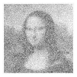
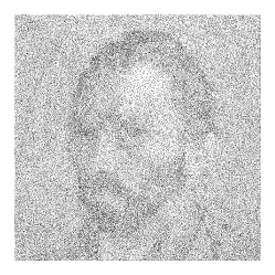
(a)			(b)
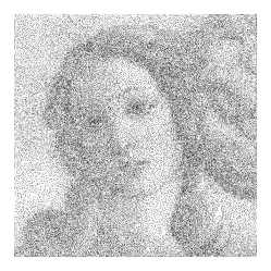
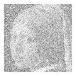
(c)			(d)

Figure 2: Four classical art based TSP instances (downloadable from http://www.math.uwaterloo.ca/tsp/data/art/), (a) da Vinci’s Mona Lisa (100K cities), (b) Van Gogh’s Self Portrait 1889 (120K cities), (c) Botticelli’s The Birth of Venus (140K cities) and (d) Vermeer’s Girl with a Pearl Earring (200K cities)

As previously, PartialACO will be run for 100,00 iterations with 16 ants and results averaged over 10 random runs. Moreover, given the large scale of the problems under consideration, the maximum aspect of the $l_{best}$ tour that can be modified by an ant is now reduced to just 1% of the number of cities which for the Mona Lisa TSP is still 1,000 cities. 2-opt search will be performed with a probability of 0.001. However, 2-opt is a computationally expensive algorithm of $O(n^{2})$ complexity. Consequently, 2-opt will be restricted to only considering swapping edges that are within 500 cities of each other in the current tour. This reduces the runtime of 2-opt significantly although slightly reduces its effectiveness.

Table 8: Results from testing PartialACO on four art TSP instances. Accuracy expressed as percentage difference from best known tour. Results averaged over 10 runs.

TSP Instance	Accuracy (% Error)			Execution Time (in hours)
	Average	Best	Worst
mona-lisa100K	$5.45$ p m 0.07	$5.36$	$5.58$	$1.07$ p m 0.02
vangogh120K	$5.82$ p m 0.10	$5.70$	$6.01$	$1.45$ p m 0.03
venus140K	$5.81$ p m 0.14	$5.60$	$6.05$	$2.09$ p m 0.06
earring200K	$7.20$ p m 0.18	$6.91$	$7.39$	$5.06$ p m 0.14

Table 9: Results from testing standard P-ACO against the four large art based TSP instances for the timings reported in Table 8. Accuracy is expressed as the percentage difference from the best known solution. The number of iterations is shown enabling a speedup of PartialACO to be ascertained. Results averaged over 10 runs.

TSP Instance	Accuracy (% Error)			Average Iterations	Relative Speedup by PartialACO
	Average	Best	Worst
mona-lisa100K	$13.50$ p m 0.49	$12.62$	$14.46$	$248.10$ p m 4.41	403.06x
vangogh120k	$14.04$ p m 0.54	$13.25$	$15.07$	$157.00$ p m 1.76	636.94x
venus140k	$14.48$ p m 2.24	$13.04$	$20.71$	$105.30$ p m 3.77	949.67x
earring200k	$16.71$ p m 3.25	$13.97$	$21.46$	$83.40$ p m 0.52	1199.04x

The results of executing the PartialACO technique on the large scale TSP instances are shown in Table 8 whereby it can be observed that tours with an average error ranging between 5-7% of the best known optima are found. Regarding runtime, PartialACO finds these tours with just a few hours of computational time using a single multi-core CPU. To clearly demonstrate the effectiveness of PartialACO a comparison is made with the standard P-ACO approach. Given the likely increase in runtime it would not be feasible to execute for 100,000 iterations. Consequently, a time limited approach is used whereby the standard P-ACO approach is run for the same degree of time as the results from Table 8 and the number of iterations achieved recorded which provides a relative speedup achieved by PartialACO. These results are shown in Table 9 whereby it can be observed that much worse accuracy is achieved which is to be expected as P-ACO only ran for a few hundred iterations. Furthermore, a speedup of up to 1200x is demonstrated by PartialACO. To understand this speedup the number of required edge comparisons to unvisited cities to determine which city to visit next by an ant building a tour must be considered. The number of comparisons an ant will make relates to a triangle progression sequence defined by $(n(n+1))/2$. Thus, an ant building a complete tour for a 100k city problem will perform approximately $5\times 10^{9}$ edge comparisons. However, if only 1% of a tour is modified an ant will only perform $5\times 10^{5}$ comparisons, a 10,000 fold efficiency saving. However, not all of this saving will be realised as a result of computational factors such as the use of 2-opt. The 10,000 fold efficiency only applies to the tour construction aspect of ACO hence the lower reported speedups.

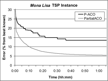
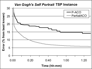
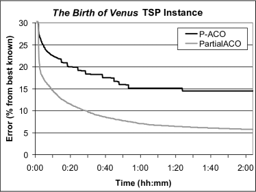
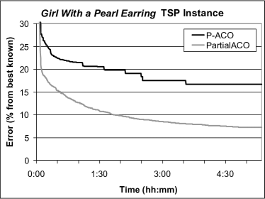
Figure 3: The average convergence rates over time for the P-ACO and PartialACO techniques and each of the art based TSP instances

Further evidence of the effectiveness of PartialACO is demonstrated by considering the convergence rates over time for each of the art based TSP instances as shown in Figure 3. PartialACO clearly converges much faster than the P-ACO approach for all four problems. Indeed, inspection of the largest problem instance, The Girl With the Pearl Earring, shows that the PartialACO technique achieves the same accuracy in minutes that P-ACO takes hours to achieve. This convergence speed is simply as a result of PartialACO being able to perform many more iterations of the ant tours, indeed thousands, in a short space of time. In fact, it can be argued that in terms of iterations PartialACO converges slower but given that time is a more important factor, PartialACO is the better approach.

6 Related Work

It is acknowledged that ACO is computationally intensive. Indeed, even the original author of ACO was aware of the computational complexity proposing a variant known as Ant Colony System (ACS) [7] whereby the neighbourhood of unvisited cities is restricted. A candidate list approach is used whereby at each decision point made by an ant, only the closest cities are considered. If these have already been visited then normal ACO used. This approach significantly reduces the computational complexity. ACS is also similar to PartialACO in that with a high probability an ant takes the edge with the greatest level of combined pheromone and heuristic information improving the speed. However, ACS still requires a full pheromone matrix and to needs to search for the edge with the greatest level to choose the next city to visit.

The main area of research into speeding up ACO though has been through parallel implementations. ACO is naturally parallel such that ants can construct tours simultaneously. Early works such as Bullnheimer et al. [2], Delisle et al. [6] and Randall and Lewis [13] relied on distributing ants to processors using a master-slave methodology. In recent years the focus on speeding up ACO has been on utilising Graphical Processor Units (GPUs) consisting of thousands of SIMD processors. Bai et al. were the first to implement MAX-MIN ACO for the TSP on a GPU achieving a 2.3x speedup [1]. More notable works include DeléVacq et al. who compare parallelisation strategies for MAX-MIN ACO on GPUs [5], Cecelia et al. who present an Independent Roulette approach to better exploit data parallelism for ACO on GPUs [3] and Dawson and Stewart who introduce a double spin ant decision methodology when using GPUs [4]. However, ACO is not ideally suited to GPUs and these papers can only report speedups ranging between 40-80x over a sequential implementation.

7 Conclusions

This paper has addressed the issues associated with applying ACO to large scale TSP instances, namely reducing memory constraints and substantially increasing execution speed. A new variant of ACO was introduced, PartialACO, based upon P-ACO which dispenses with the pheromone matrix, the memory overhead. Moreover, PartialACO only partially modifies the best tour found by each ant akin to crossover in GAs. PartialACO was demonstrated to significantly improve the computational speed of ACO and the accuracy by reducing the computational complexity and the probabilistic chance of ants making poor choices of cities to visit. Consequently, PartialACO was applied to large scale TSP instances of up to 200K cities achieving accuracy of 5-7% of the best known tours with a speed of up to 1200 times faster than that of standard P-ACO. PartialACO is a first step to deploying ACO on large scale TSP instances and further work is required to improve its accuracy to compete with a GA approach [12] although it should be noted that this work uses a supercomputer. Further analysis of the parameters balancing speed vs. accuracy could help to improve the technique such as reducing the maximum permissable modification of tours for speed and increasing the iterations. Moreover, a dynamic approach may be best whereby initially only small modifications are allowed but as time progresses the permissible modification increases to avoid being trapped in local optima.

8 Acknowledgement

This is a pre-print of a contribution published in Chao F., Schockaert S., Zhang Q. (eds) Advances in Computational Intelligence Systems. UKCI 2017, Advances in Intelligent Systems and Computing, vol. 650 published by Springer. The definitive authenticated version is available online via https://doi.org/10.1007/978-3-319-66939-7_9.

References

- [1] Bai, H., OuYang, D., Li, X., He, L., Yu, H.: MAX-MIN ant system on GPU with CUDA. In: Innovative Computing, Information and Control (ICICIC), 2009 Fourth International Conference on. pp. 801–804. IEEE (2009)
- [2] Bullnheimer, B., Kotsis, G., Strauß, C.: Parallelization strategies for the ant system. In: High Performance Algorithms and Software in Nonlinear Optimization, pp. 87–100. Springer (1998)
- [3] Cecilia, J.M., García, J.M., Nisbet, A., Amos, M., Ujaldón, M.: Enhancing data parallelism for ant colony optimization on GPUs. Journal of Parallel and Distributed Computing 73(1), 42–51 (2013)
- [4] Dawson, L., Stewart, I.: Improving ant colony optimization performance on the GPU using CUDA. In: Evolutionary Computation (CEC), 2013 IEEE Congress on. pp. 1901–1908. IEEE (2013)
- [5] DeléVacq, A., Delisle, P., Gravel, M., Krajecki, M.: Parallel ant colony optimization on graphics processing units. Journal of Parallel and Distributed Computing 73(1), 52–61 (2013)
- [6] Delisle, P., Krajecki, M., Gravel, M., Gagné, C.: Parallel implementation of an ant colony optimization metaheuristic with OpenMP. In: Proceedings of the 3rd European Workshop on OpenMP (EWOMP 01), Barcelona, Spain (2001)
- [7] Dorigo, M., Gambardella, L.M.: Ant colony system: a cooperative learning approach to the traveling salesman problem. IEEE Transactions on evolutionary computation 1(1), 53–66 (1997)
- [8] Dorigo, M., Stützle, T.: Ant Colony Optimization. Bradford Company, Scituate, MA, USA (2004)
- [9] Eberhart, R., Kennedy, J.: A new optimizer using particle swarm theory. In: Micro Machine and Human Science, 1995. MHS’95., Proceedings of the Sixth International Symposium on. pp. 39–43. IEEE (1995)
- [10] Guntsch, M., Middendorf, M.: A population based approach for ACO. In: Workshops on Applications of Evolutionary Computation. pp. 72–81. Springer (2002)
- [11] Holland, J.H.: Adaptation in natural and artificial systems: an introductory analysis with applications to biology, control, and artificial intelligence. MIT Press (1975)
- [12] Honda, K., Nagata, Y., Ono, I.: A parallel genetic algorithm with edge assembly crossover for 100,000-city scale TSPs. In: Evolutionary Computation (CEC), 2013 IEEE Congress on. pp. 1278–1285. IEEE (2013)
- [13] Randall, M., Lewis, A.: A parallel implementation of ant colony optimization. Journal of Parallel and Distributed Computing 62(9), 1421–1432 (2002)