Rates of Convergence of Spectral Methods for Graphon Estimation

Abstract

This paper studies the problem of estimating the grahpon model – the underlying generating mechanism of a network. Graphon estimation arises in many applications such as predicting missing links in networks and learning user preferences in recommender systems. The graphon model deals with a random graph of $n$ vertices such that each pair of two vertices $i$ and $j$ are connected independently with probability $\rho\times f(x_{i},x_{j})$, where $x_{i}$ is the unknown $d$-dimensional label of vertex $i$, $f$ is an unknown symmetric function, and $\rho$ is a scaling parameter characterizing the graph sparsity. Recent studies have identified the minimax error rate of estimating the graphon from a single realization of the random graph. However, there exists a wide gap between the known error rates of computationally efficient estimation procedures and the minimax optimal error rate.

Here we analyze a spectral method, namely universal singular value thresholding (USVT) algorithm, in the relatively sparse regime with the average vertex degree $n\rho=\Omega(\log n)$. When $f$ belongs to Hölder or Sobolev space with smoothness index $\alpha$, we show the error rate of USVT is at most $(n\rho)^{-2\alpha/(2\alpha+d)}$, approaching the minimax optimal error rate $\log(n\rho)/(n\rho)$ for $d=1$ as $\alpha$ increases. Furthermore, when $f$ is analytic, we show the error rate of USVT is at most $\log^{d}(n\rho)/(n\rho)$. In the special case of stochastic block model with $k$ blocks, the error rate of USVT is at most $k/(n\rho)$, which is larger than the minimax optimal error rate by at most a multiplicative factor $k/\log k$. This coincides with the computational gap observed for community detection. A key step of our analysis is to derive the eigenvalue decaying rate of the edge probability matrix using piecewise polynomial approximations of the graphon function $f$.

1 Introduction

Many modern systems and datasets can be represented as networks with vertices denoting the objects and edges (possibly weighted or labelled) encoding their interactions. Examples include online social networks such as Facebook friendship network, biological networks such as protein-protein interaction networks, and recommender systems such as movie rating datasets. A key task in network analysis is to estimate the underlying network generating mechanism, i.e., how the edges are formed in a network. It is useful for many important applications such as studying network evolution over time [44], predicting missing links in networks [42, 2, 19], learning hidden user prefererences in recommender systems [46], and correcting errors in crowd-sourcing systems [36]. In practice, we usually only observe a very small fraction of edge connections in these networks, which obscures the underlying network generating mechanism. For example, around $80\%$ of the molecular interactions in cells of Yeast [52] are unknown. In Netflix movie dataset, about $99\%$ of movie ratings are missing and the observed ratings are noisy.

In this paper, we are interested in understanding when and how the underlying network generating mechanism can be efficiently inferred from a single snapshot of a network. We assume the observed network is generated according to the graphon model [40]. Graphon is a powerful network model that plays a central role in the study of large networks. It was originally developed as a limit of a sequence of graphs with growing sizes [39], and has been applied to various network analysis problems ranging from testing graph properties to counting homomorphisms to charactering distances between two graphs [39, 10, 11] to detecting communities [6]. Concretely, given $n$ vertices, the edges are generated independently, connecting each pair of two distinct vertices $i$ and $j$ with a probability

$$M_{ij}=f(x_{i},x_{j}),$$ (1)

where $x_{i}\in{\mathcal{X}}$ is the latent feature vector of vertex $i$ that captures various characteristics of vertex $i$; $f:{\mathcal{X}}\times{\mathcal{X}}\to[0,1]$ is a symmetric function called graphon. We assume no self loop and set $M_{ii}=0$ for $1\leq i\leq n$. We further assume the feature vectors $x_{i}$’s are drawn i.i.d. from the measurable space ${\mathcal{X}}$ according to a probability distribution $\mu$. Graphon model encompasses many existing network models as special cases. Setting $f$ to be a constant $p$, it gives rise to Erdős-Rényi random graphs [17], where each edge is formed independently with probability $p$. In the case where ${\mathcal{X}}$ is a discrete set of $k$ elements, the model specializes to the stochastic block model with $k$ blocks [25], where each vertex belongs to a community, and the edge probability between $i$ and $j$ depends only on which communities they are in. If ${\mathcal{X}}$ is a Euclidean space of dimension $d$ and $f(x_{i},x_{j})$ is a function of the Euclidean distance $\|x_{i}-x_{j}\|$, then the grahon model reduces to the latent space model [24, 23].

To further model the partial observation of the networks, we assume every edge is observed independently with probability $\rho\in[0,1]$, where $\rho$ may converge to $0$ as $n\to\infty$. Let $A$ denote the adjacency matrix of the resulting observed graph with $A_{ii}=0$ by convention. Then conditional on $x=(x_{1},\ldots,x_{n})$, for $1\leq i<j\leq n$, $A_{ij}=A_{ji}$ are independently distributed as ${\rm Bern}\left(\rho M_{ij}\right)$. The problem of interest is to estimate the underlying network generating mechanism – either the edge probability matrix $M$ or the graphon $f$ – from a single observation of the network $A.$ It turns out that estimating $M$ and estimating $f$ are the twin problems, and the result in the former can be readily extended to the latter, as shown in [28, Section 3]. Thus in this paper we shall focus on estimating the edge probability matrix $M$. To measure the quality of an estimator $\widehat{M}$ of $M$, we consider the mean-squared error:

$$\textup{MSE}(\widehat{M})=(1/n^{2})\mathbb{E}[\|M-\widehat{M}\|_{F}^{2}],$$ (2)

which is the expected difference between the estimated edge probability matrix and the true one in the normalized Frobenius norm. Furthermore, to investigate the fundamental estimation limits, we take the decision-theoretic approach and consider the minimax mean-squared error: $\inf_{\widehat{M}}\sup_{M\in{\mathcal{M}}}\textup{MSE}(\widehat{M})$, where ${\mathcal{M}}$ denotes a set of admissible edge probability matrices. The minimax estimation error depends on the smoothness of graphon $f$, the structure of latent space $({\mathcal{X}},\mu)$, and the observation probability $\rho.$

There is a recent surge of interest in graphon estimation and various procedures have been proposed and analyzed [20, 28, 19, 49, 2, 51, 13, 12, 53, 9, 29]. A recent line of work [20, 28, 19] has characterized the minimax error rate in certain special regimes. In particular, for stochastic block model with $k$ blocks, it is shown that the minimax error rate is $\frac{k^{2}}{n^{2}\rho}+\frac{\log k}{n\rho}$. For fully observed graphons with $f$ being Hölder smooth on ${\mathcal{X}}=[0,1]$ and $\rho=1$, the minimax error rate turns out be $n^{-1}\log k+n^{-2\alpha/(\alpha+1)},$ where $\alpha$ is the smoothness index of $f$. This result was extended by [28, 19] to sparse regimes with $\rho\to 0$.

From a computational perspective, the problem appears to be much harder and far less well-understood. In the special case where $f$ is $\alpha$-Hölder smooth on ${\mathcal{X}}=[0,1]$, a universal singular value thresholding (USVT) algorithm is shown in [14] to achieve an error rate of $n^{-1/3}\rho^{-1/2}$. However, this performance guarantee is rather weak and far from the minimax optimal rate $\log(n\rho)/(n\rho)$. A similar spectral method is shown in [50] to achieve a vanishing MSE when $n\rho\gg\log n$ but without an explicit characterization of the rate of the convergence. The nearest-neighbor based approach is analyzed in [46] under a stringent assumption $n\rho\gg\sqrt{n}$. A simple degree sorting algorithm is shown to achieve an error rate of $\left(\log(n\rho)/(n\rho)\right)^{\alpha/(4\alpha+d)}$ for $\alpha\in(0,1]$ under the restrictive assumption that $\int_{0}^{1}f(x,y){\rm d}y$ is strictly monotone in $x$.

In summary, despite the recent significant effort devoted to developing fundamental limits and efficient algorithms for graphon estimation, an understanding of the statistical and computational aspects of graphon estimation is still lacking. In particular, there is a wide gap between the known performance bounds of computationally efficient procedures and the minimax optimal estimation rate. This raises a fundamental question:

Is there a polynomial-time algorithm that is guaranteed to achieve the minimax optimal rate?

In this paper, we provide a partial answer to this question by analyzing the universal singular value thresholding (USVT) algorithm proposed by Chatterjee [14]. The universal singular value thresholding is a simple and versatile method for structured matrix estimation and has been applied to a variety of different problems such as ranking [45]. It truncates the singular values of $A$ at a threshold slightly above the spectral norm $\|A-\mathbb{E}\left[A\right]\|$, and estimates $M$ by a properly rescaled $A$ after truncation. It is computationally efficient when $A$ is sparse. However, its performance guarantee established in [14] is rather weak: the total number of observed edges needs to be much larger than $n^{(2d+2)/(d+2)}$ to attain a vanishing MSE. In contrast, our improved performance bound shows that the total number of observed edges only needs to be a constant factor larger than $n\log n$, irrespective of the latent space dimension $d$.

More formally, by assuming the average vertex degree $n\rho=\Omega(\log n)$ and ${\mathcal{X}}$ is a compact subset in ${\mathbb{R}}^{d}$, the mean-squared error rate of USVT is shown to be upper bounded by $(n\rho)^{-2\alpha/(2\alpha+d)}$, when $f$ belongs to either $\alpha$-smooth Hölder function class ${\mathcal{H}}(\alpha,L)$ or $\alpha$-smooth Sobolev space ${\mathcal{S}}(\alpha,L)$. Interestingly, our convergence rate of USVT closely resembles the typical rate $N^{-2\alpha/(2\alpha+d)}$ in the nonparametric regression problem [47], where $N$ denotes the number of observations and $d$ is the function dimension. When $d=1$, the convergence rate of USVT is approaching the minimax optimal rate $\log(n\rho)/(n\rho)$ as $f$ becomes smoother, i.e., $\alpha$ increases. In fact, we show that if $f$ is analytic with infinitely many times differentiability, then the error rate is upper bounded by $\log^{d}(n\rho)/(n\rho).$

In the special case of stochastic block model with $k$ blocks, the error rate of USVT is shown to be $k/(n\rho)$, which is larger than the optimal minimax rate by at most a multiplicative factor $k/\log k$. This factor coincides with the ratio of the Kesten-Stigum threshold and information-theoretic threshold for community detection [5, 1, 4]. Based on compelling but non-rigorous statistical physics arguments, it is believed that no polynomial-time algorithms are able to detect the communities between the KS-threshold and IT-threshold [43]. This coincidence indicates that $k/(n\rho)$ may be the optimal estimation rate among all polynomial-time algorithms, and the minimax optimal rate may not be attainable in polynomial-time. During the preparation of this manuscript, we became aware of an earlier arXiv preprint [29, Proposition 4] which also derives the error rate of $k/(n\rho)$.

Our proof incorporates three interesting ingredients. One is a characterization of the estimation error of USVT in terms of the tail of eigenvalues of $M$, and the spectral norm of the noise perturbation $\|A-\mathbb{E}\left[A\right]\|$, see e.g., [45, Lemma 3]. The second one is a high-probability upper bound on $\|A-\mathbb{E}\left[A\right]\|$ using matrix concentration inequalities initially developed by [18]. The last but most important one is a characterization of the tail of eigenvalues of $M$ using piecewise polynomial approximations of $f$, which were originally used to study the spectrum of integral operators defined by $f$ [7, 8]. The piecewise constant approximations of $f$ have appeared in the previous work on graphon estimation [14, 20, 28], and are sufficient for the purpose of deriving sharp minimax estimation rates because the smoothness of $f$ beyond $\alpha=1$ does not improve the rates. However, piecewise degree-$\lfloor\alpha\rfloor$ polynomial approximations are needed for showing USVT to achieve a faster converging rate as $\alpha$ increases.

Notation

Given a measurable space ${\mathcal{X}}$ endowed with measure $\mu$, let ${\mathcal{L}}^{2}({\mathcal{X}},\mu)$ denote the space of functions $f:{\mathcal{X}}\to{\mathbb{R}}$ such that $\|f\|_{2}=\left(\int_{{\mathcal{X}}}|f|^{2}{\rm d}\mu\right)^{1/2}<\infty$. When $\mu$ is the Lebesgue measure, we write ${\mathcal{L}}^{2}({\mathcal{X}})$ for simplicity. Let ${\mathbb{R}}^{d}$ denote the $d$-dimensional Euclidean space. For a vector $x\in{\mathbb{R}}^{d}$, let $\|x\|_{2}$ denote its $\ell_{2}$ norm and $\|x\|_{\infty}=\max_{1\leq i\leq d}|x_{i}|$ denote its $\ell$-infinity norm. For any matrix $M$, let $\|M\|$ denote its spectral norm and $\|M\|_{F}$ denote its Frobenius norm. Logarithms are natural and we adopt the convention $0\log 0=0$.

For any positive integer $n$, let $[n]=\{1,\ldots,n\}$. For any positive constant $\alpha$, let $\lfloor\alpha\rfloor$ denotes the largest integer strictly smaller than $\alpha$. For two real numbers $\alpha$ and $\beta$, let $\alpha\wedge\beta=\min\{\alpha,\beta\}$ and $\alpha\vee\beta=\max\{\alpha,\beta\}$. For any set $T\subset[n]$, let $|T|$ denote its cardinality and $T^{c}$ denote its complement. If $\kappa=(\kappa_{1},\ldots,\kappa_{d})$ is a multi-index with $\kappa_{i}\in{\mathbb{N}}$, then $|\kappa|=\sum_{i=1}^{d}\kappa_{i}$, $\kappa!=\prod_{i=1}^{d}\kappa_{i}!$, and $x^{\kappa}=\prod_{i=1}^{d}x_{i}^{\kappa_{i}}$ for a vector $x\in{\mathbb{R}}^{d}.$ We use standard big $O$ notations, e.g., for any sequences $\{a_{n}\}$ and $\{b_{n}\}$, $a_{n}=\Theta(b_{n})$ or $a_{n}\asymp b_{n}$ if there is an absolute constant $c>0$ such that $1/c\leq a_{n}/b_{n}\leq c$. Throughout the paper, we say an event occurs with high probability when it occurs with a probability tending to one as $n\to\infty$.

2 Main results

To describe our main results, we first recall the universal singular value thresholding (USVT) algorithm proposed in [14]. Note that according to the graphon model (1), the edge probability matrix $M$ may not be of low-rank. Nevertheless, it is possible that the singular values of $M$, or equivalently magnitudes of eigenvalues, drop off fast enough and as a consequence $M$ is approximately low-rank. If this is indeed the case, then a natural idea to estimate $M$ is via low-rank approximations of $A$. In particular, USVT truncates the singular values of $A$ at a proper threshold $\tau$, and estimates $M$ by the rescaled $A$ after truncation.

Algorithm 1 Universal Singular Value Thresholding (USVT) [14]

1:  Input: $A\in{\mathbb{R}}^{n\times n}$, $\rho\in[0,1]$ and a threshold $\tau>0$.

2:  Let $A=\sum_{i=1}^{n}s_{i}u_{i}v_{i}^{\top}$ be its singular value decomposition with $s_{1}\geq s_{2}\geq\cdots\geq s_{n}$.

3:  Let $S$ be the set of “thresholded” singular values:

$$S=\{i:s_{i}\geq\tau\}.$$

4:  Let

$$\widehat{A}=\sum_{i\in S}s_{i}u_{i}v_{i}^{\top}$$

and $\widetilde{M}=\widehat{A}/\rho.$

5:  Output a matrix $\widehat{M}\in[0,1]^{n\times n}$ such that $\widehat{M}_{ii}=0$ for all $i\in[n],$ and for $1\leq i<j\leq n$, $\widehat{M}_{ij}=\widehat{M}_{ji}$ and

$$\widehat{M}_{ij}=\begin{cases}\widetilde{M}_{ij},&\quad\text{ if }\;\widetilde{M}_{ij}\in[0,1]\\ 1,&\quad\text{ if }\;\widetilde{M}_{ij}>1\\ 0,&\quad\text{ if }\;\widetilde{M}_{ij}<0.\end{cases}$$

Note that Algorithm 1 applies hard-thresholding to the singular values of $A$. Alternatively, we can use soft-thresholding [31] and let $\widehat{A}=\sum_{i\in S}(s_{i}-\tau)u_{i}v_{i}^{\top}$. Our main results with the hard-thresholding also apply to the soft-thresholding. As argued in [14], the cut-off threshold $\tau$ is chosen to be slightly above $\|A-\mathbb{E}\left[A\right]\|$, so that noise is suppressed and signals corresponding to large singular values of $\mathbb{E}\left[A\right]$ are maintained. Since conditional on $\mathbb{E}\left[A\right]$, $A$ is a random matrix with independent entries bounded in $[0,1]$ of variance at most $\rho$, it is expected that $\|A-\mathbb{E}\left[A\right]\|\lesssim\sqrt{n\rho}$ with high probability, in view of standard matrix concentration inequalities. This turns out to be true if the observed graph is not too sparse, i.e., there exists a positive constant $C$ such that

$$n\rho\geq C\log n.$$ (3)

However, when the observed graph is sparse with $n\rho=o(\log n)$, due to the existence of high-degree vertices, $\|A-\mathbb{E}\left[A\right]\|\gg\sqrt{n\rho}$ with high probability [21, Appendix A].

Motivated by the discussion above, we shall focus on the relatively sparse regime where (3) holds, and set $\tau=c_{0}\sqrt{n\rho}$ for a positive large constant $c_{0}$, whose value depends on the constant $C$ in (3). It is known that with high probability,

$$\|A-\mathbb{E}\left[A\right]\|\leq\kappa\sqrt{nr},$$

where

$$\kappa=\begin{cases}4+o(1)&n\rho=\omega(\log n)\\ 2+o(1)&n\rho=\omega(\log^{4}n)\end{cases},$$ (4)

see, e.g.,  [22, Lemma 30]. Hence, the constant $c_{0}$ can be set to be a universal constant strictly larger than $4$ in the case of $n\rho\gg\log(n)$ and $2$ in the case of $n\rho\gg\log^{4}(n)$. Notably, in these cases, the cut-off threshold $\tau$ is universal, independent of the underlying graphon $f$. Our first result provides an upper bound to the estimation error of USVT.

Theorem 1.

Consider the relatively sparse regime where (3) holds. For all $c>0$ there exists a positive constant $\kappa$ such that if $\tau=(1+\delta)\kappa\sqrt{n\rho}$ for a fixed constant $\delta>0$, then conditional on $M$, with probability at least $1-n^{-c}$,

$$\frac{1}{n^{2}}\|\widehat{M}-M\|_{F}^{2}\leq 16(1+\delta)^{2}\min_{0\leq r\leq n}\left(\frac{\kappa^{2}r}{n\rho}+\frac{1}{n^{2}\delta^{2}}\sum_{i\geq r+1}\lambda_{i}^{2}(M)\right).$$

Furthermore, it follows that

$$\textup{MSE}(\widehat{M})\leq 16(1+\delta)^{2}\min_{0\leq r\leq n}\left(\frac{\kappa^{2}r}{n\rho}+\frac{1}{n^{2}\delta^{2}}\sum_{i\geq r+1}\mathbb{E}\left[\lambda_{i}^{2}(M)\right]\right)+n^{-c}.$$

Theorem 1 gives an upper bound to the estimation error of USVT in terms of the tail of eigenvalues of $M$ and the observation probability $\rho.$ The upper bound invovles minimization of a sum of two terms over integers $0\leq r\leq n$: the first term $r/(n\rho)$ can be viewed as the estimation error for a rank-$r$ matrix; the second term $n^{-2}\sum_{i\geq r+1}\lambda_{i}^{2}(M)$ is the tail of eigenvalues of $M$ and charaterizes the approximation error of $M$ by the best rank-$r$ matrix. The optimal $r$ is chosen to achieve the best trade-off between the estimation error and the approximaiton error. Moreover, a lighter tail of eigenvalues of $M$ implies a faster convergence rate of the estimation error. To characterize different tails of eigenvalues of $M$, we introduce the following definitions of polynomial and super-polynomial decays.

Definition 1 (Polynomial decay).

We say the eigenvalues of $M$ asymptotically satisfy a polynomial decay with rate $\beta>0$ if for all integers $0\leq r\leq n-1$,

$$\frac{1}{n^{2}}\sum_{i\geq r+1}\mathbb{E}\left[\lambda_{i}^{2}(M)\right]\leq c_{0}r^{-\beta}+c_{1}n^{-1},$$

where $c_{0}$ and $c_{1}$ are two constants independent of $n$ and $r.$

Definition 2 (Super-polynomial decay).

We say the eigenvalues of $M$ asymptotically satisfy a super-polynomial decay with rate $\alpha>0$ if for all integers $0\leq r\leq n-1$,

$$\frac{1}{n^{2}}\sum_{i\geq r+1}\mathbb{E}\left[\lambda_{i}^{2}(M)\right]\leq c_{0}e^{-c_{2}r^{\alpha}}+c_{1}n^{-1},$$

where $c_{0},c_{1},c_{2}$ are constants independent of $n$ and $r.$

We remark that in the above two definitions, we allow for a residual term $c_{1}n^{-1}$, which is responsible for the contribution of diagonal entries of $M$. According to Theorem 1, this residual term only induces an additional $n^{-1}$ error in the upper bound to MSE and will not affect our main results. The following corollary readily follows from Theorem 1 by choosing the optimal $r$ according to the decay rates of eigenvalues of $M$.

Corollary 1.

Consider the relatively sparse regime where (3) holds and suppose the eigenvalues of $M$ satisfy a polynomial decay with rate $\beta>0$. Then there exists a positive constant $\kappa>0$ such that if $\tau=(1+\delta)\kappa\sqrt{n\rho}$ for a fixed constant $\delta>0$,

$$\textup{MSE}(\widehat{M})\leq c^{\prime}(n\rho)^{-\frac{\beta}{\beta+1}}.$$

If instead the eigenvalues of $M$ satisfy a super-polynomial decay with rates $\alpha>0$, then

$$\textup{MSE}(\widehat{M})\leq c^{\prime}\frac{\left(\log(n\rho)\right)^{1/\alpha}}{n\rho},$$

where $c^{\prime}$ is a positive constant independent of $n$.

Proof.

The first conclusion follows from Theorem 1 by choosing $c=1$ and $r=\lfloor(n\rho)^{1/(\beta+1)}\rfloor$ and the second one follows by choosing $c=1$ and $r=\lfloor\left(\log(n\rho)/c_{2}\right)^{1/\alpha}\rfloor$. ∎

Next we specialize our general results in different settings by deriving the decay rates of eigenvalues of $M.$

2.1 Stochastic block model

We first present results on the rate of convergence in the stochastic block model setting, where $x_{i}\in\{1,2,\ldots,k\}$ indicating which community that vertex $i$ belongs to. In this case, $M_{ij}$ only depends on the communities of vertex $i$ and vertex $j$, and $M$ has rank at most $k$.

Theorem 2.

Assume (3) holds under the stochastic block model with $k$ blocks, Then there exists a positive constant $\kappa>0$ such that if $\tau=(1+\delta)\kappa\sqrt{n\rho}$ for some fixed constant $\delta>0$,

$$\textup{MSE}(\widehat{M})\leq c^{\prime\prime}\left[\frac{k}{n\rho}\wedge 1\right].$$

where $c^{\prime\prime}$ is a positive constant depending on $\kappa$ and $\delta.$

Proof.

Under the stochastic block model, $M$ is of rank at most $k$. Thus $\lambda_{i}(M)=0$ for all $i\geq k+1$. Moreover, since $M_{ij}\in[0,1]$, it follows that $\sum_{i=1}^{k}\lambda_{i}^{2}(M)=\|M\|_{F}^{2}\leq n^{2}$. Applying Theorem 1 with $r=0$ and $r=k$ yields the desired result. ∎

Theorem 2 shows that the convergence rate of MSE of USVT is at most $\frac{k}{n\rho}\wedge 1$, while the previous result in [14] establishes that the convergence rate is at most $\sqrt{k/n}$ for $\rho=1$. During the preparation of this manuscript, we became aware of an earlier arXiv preprint [29, Proposition 4] which also proves the error rate of $k/(n\rho).$

The minimax optimal rate derived in [28, 19] is $\left(\frac{k^{2}}{n^{2}\rho}+\frac{\log k}{n\rho}\right)\wedge 1$. Hence, the error rate of USVT is larger than the minimax optimal rate by at most a multiplicative factor of $k/\log k$, which resembles the computational gap observed for community detection [5, 1] and the related high-dimensional statistical inference problems discussed in [4]. In particular, it is shown in [5, 1] that estimation better than randomly guessing is attainable efficiently by spectral methods when above the Kesten-Stigum threshold, while it is information-theoretically possible even strictly below the KS threshold by a multiplicative factor $k/\log k$. In between the KS threshold and information-theoretic threshold, non-trivial estimation is information-theoretically possible but believed to require exponential time. The same conclusion also holds for exact community recovery as shown in [15]. Due to this coincidence, it is tempting to believe that $\frac{k}{n\rho}\wedge 1$ might be the optimal estimation rate among all polynomial-time algorithms; however, we do not have a proof.

2.2 Smooth graphon

Next we proceed to the smooth graphon setting. We assume ${\mathcal{X}}=[0,1)^{d}$ for simplicity. There are various notions to characterize the smoothness of graphon. In this paper, we focus on the following two notions, which are widely adopted in the non-parametric regression literature [47].

Given a function $g:{\mathcal{X}}\to{\mathbb{R}}$ and a multi-index $\kappa$, let

$$\nabla_{\kappa}g(x)=\frac{\partial^{|\kappa|}g(x)}{(\partial x)^{\kappa}}$$ (5)

denote its partial derivative whenever it exists.

Definition 3 (Hölder class).

Let $\alpha$ and $L$ be two positive numbers. The Hölder class ${\mathcal{H}}(\alpha,L)$ on ${\mathcal{X}}$ is defined as the set of functions $g:{\mathcal{X}}\to{\mathbb{R}}$ whose partial derivatives satisfy

$$\sum_{\kappa:|\kappa|=\lfloor\alpha\rfloor}\frac{1}{\kappa!}\left|\nabla_{\kappa}g(x)-\nabla_{\kappa}g(x^{\prime})\right|\leq L\|x-x^{\prime}\|_{\infty}^{\alpha-\lfloor\alpha\rfloor}.$$ (6)

Note that if $\alpha\in(0,1]$, then (6) is equivalent to the Lip-$\alpha$ condition:

$$|g(x)-g(x^{\prime})|\leq L\|x-x^{\prime}\|_{\infty}^{\alpha}.$$ (7)

One can also measure the smoothness with respect to the underlying measure $\mu$. This leads to the consideration of Sobolev space. For ease of exposition, we assume $\mu$ is the Lebesgue measure. The main results can be extended to more general Borel measures.

Definition 4 (Sobolev space).

Let $\alpha$ and $L$ be two positive numbers. The Sobolev space $S(\alpha,L)$ on $({\mathcal{X}},\mu)$ is defined as the set of functions $g:{\mathcal{X}}\to{\mathbb{R}}$ whose partial derivatives satsify

$$\sum_{\kappa:|\kappa|=\alpha}\int_{{\mathcal{X}}}\|\nabla_{\kappa}g(x)\|_{2}^{2}\;{\rm d}x\leq L^{2},\quad\text{for integral }\alpha,$$

and

$$\sum_{\kappa:|\kappa|=\lfloor\alpha\rfloor}\int_{{\mathcal{X}}\times{\mathcal{X}}}\frac{\|\nabla_{\kappa}g(x)-\nabla_{\kappa}g(y)\|_{2}^{2}}{\|x-y\|_{2}^{2(\alpha-\lfloor\alpha\rfloor)+d}}\;{\rm d}x{\rm d}y\leq L^{2},\quad\text{for non-integral }\alpha.$$

Note that the graphon $f(x,y)$ is a bi-variate function. We treat it as a function of $x$ for every fixed $y$, and introduce the following two conditions on $f$.

Condition 1 (Hölder condition on $f$).

There exist two positive numbers $\alpha$ and $L$ such that $f(\cdot,y)\in{\mathcal{H}}(\alpha,L)$ for every $y\in{\mathcal{X}}$.

Condition 2 (Sobolev condition on $f$).

There exist two positive numbers $\alpha$ and $L$ such that $f(\cdot,y)\in{\mathcal{S}}(\alpha,L(y))$ for every $y$, where $L(y):{\mathcal{X}}\to{\mathbb{R}}$ satisfies that $\int_{{\mathcal{X}}}L^{2}(y){\rm d}y\leq L^{2}$.

The following key result shows that the eigenvalues of $M$ drop off to zero in a polynomial rate depending on the smoothness index $\alpha$ of $f.$

Proposition 1.

Suppose that $f$ satisfies either Condition 1 or Condition 2. Then there exists a constant $C=C(\alpha,L,d)$ only depending on $\alpha,$ $L,$ and $d$ such that for all integers $0\leq r\leq n-1$,

$$\frac{1}{n^{2}}\sum_{i\geq r+1}\mathbb{E}\left[\lambda_{i}^{2}(M)\right]\leq C(\alpha,L,d)\left(n^{-1}+r^{-2\alpha/d}\right).$$

Remark 1.

In the special case where $f$ is Hölder smooth with $\alpha=1$, Proposition 1 has been proved in [14]. In particular, it is shown in [14] that $f$ can be well-approximated by a piecewise constant function. As a consequence, $M$ can be approximated by a rank-$r$ block matrix with $r^{2}$ blocks, and the entry-wise approximation error in the squared Frobenius norm is shown to be approximately $r^{-2\alpha/d}$. The same idea can be readily extended to the case $\alpha\in[0,1]$. However, piecewise constant approximations of $f$ no longer suffice for $\alpha>1$, because Hölder smoothness condition (6) no longer implies Lip-$\alpha$ condition (7). In fact (7) with $\alpha>1$ will imply that $f\equiv C$ for some constant $C$. Instead, we show that $f$ can be well approximated by piecewise polynomials of degree $\lfloor\alpha\rfloor$.

By combining Proposition 1 with Corollary 1, we immediately get the following result on the convergence rate of the estimation error of USVT.

Theorem 3.

Under the graphon estimation model, assume (3) holds, and $f$ satisfies either Condition 1 or Condition 2. There exists a positive constant $\kappa$ such that if $\tau=(1+\delta)\kappa\sqrt{n\rho}$ for some fixed constant $\delta>0$, then

$$\textup{MSE}(\widehat{M})\leq c^{\prime\prime}(n\rho)^{-\frac{2\alpha}{2\alpha+d}},$$

where $c^{\prime\prime}$ is a positive constant independent of $n.$

Theorem 3 implies that if $f$ is infinitely many times differentiable, then the MSE of USVT converges to zero faster than $(n\rho)^{-1+\epsilon}$ for an arbitrarily small constant $\epsilon>0.$ In fact, we can prove a sharper result when $f$ is analytic, i.e., $f$ is infinitely differentiable and its Taylor series expansion around any point in its domain converges to the function in some neighborhood of the point.

Theorem 4.

Under the graphon estimation model, suppose there there exists positive constants $a$ and $b$ such that for all multi-indices $\kappa$ and all $y\in{\mathcal{X}}$

$$\sup_{x\in{\mathcal{X}}}\frac{\partial^{|\kappa|}f(x,y)}{(\partial x)^{\kappa}}\leq ba^{|\kappa|}\kappa!.$$ (8)

There exists positive constants $c_{0}$ and $c_{1}$ only depending on $a,b,d$ such that for all integers $0\leq r\leq n-1,$

$$\frac{1}{n^{2}}\sum_{i\geq r+1}\lambda_{i}^{2}(M)\leq c_{1}\left(n^{-1}+\exp\left(-c_{0}r^{1/d}\right)\right).$$ (9)

Moreover, assume (3) holds. Then there exists positive constants $c^{\prime},c^{\prime\prime}$ such that if $\tau=c^{\prime\prime}\sqrt{n\rho}$,

$$\textup{MSE}(\widehat{M})\leq c^{\prime}\frac{\log^{d}\left(n\rho\right)}{n\rho}.$$

We remark that for a fixed $y\in{\mathcal{X}}$, (8) is a sufficient and necessary condition for $f(\cdot,y)$ being analytic [33]. Note that (9) implies the eigenvalues of $M$ has a super-polynomial decay with rate $\alpha=1/d$. Its proof is based on approximating $f(\cdot,y)$ using its Taylor series truncated at degree $\ell\asymp r^{1/d}$. When $d=1$, the eigenvalues of $M$ decays to zero exponentially fast in $r$; such an exponentialy decay can be also proved via Chebyshev polynomial approximation of $f$ as shown in [38].

2.2.1 Comparison to minimax optimal rates

In this section, we compare the rates of convergence of USVT for estimating Hölder smooth graphons to the minimax optimal rates when the dimension of latent feature space $d=1$. In the dense regimes with $\rho=1$, the minimax rates of estimating Hölder smooth graphons have been derived in [20]:

$$\inf_{\widehat{M}}\sup_{f\in{\mathcal{H}}(\alpha,L)}\sup_{\mu\in{\mathcal{P}}[0,1]}\textup{MSE}(\widehat{M})\asymp\begin{cases}n^{-2\alpha/(\alpha+1)},&0<\alpha<1\\ \frac{\log n}{n},&\alpha\geq 1,\end{cases}$$

where ${\mathcal{P}}[0,1]$ denotes all probability distributions supported over $[0,1].$ The results have been extended by [28] to sparse regimes where $\rho\to 0$ as $n\to\infty.$ However, the minimax result derived in [28] contains minor errors. In particular, it is claimed that that the minimax rate is always lower bounded by $\frac{\log n}{n\rho}$. However, as we shown in Theorem 3, when $d=1$, the error rate of USVT for estimating $\alpha$-smooth graphon is at most $(n\rho)^{-2\alpha/(2\alpha+1)}$, which strictly improves over $\log n/(n\rho)$ when $n\rho\ll(\log n)^{2\alpha+1}$. Tracing the derivations in [28], we find that the correct minimax optimal rate is given by

$$\inf_{\widehat{M}}\sup_{f\in{\mathcal{H}}(\alpha,L)}\sup_{\mu\in{\mathcal{P}}[0,1]}\textup{MSE}(\widehat{M})\asymp\begin{cases}1,&n\rho=O(1)\\ \frac{\log(n\rho)}{n\rho},&\omega(1)\leq\log(n\rho)\leq\alpha\log n+(\alpha+1)\log\log n\\ (n^{2}\rho)^{-\alpha/(\alpha+1)},&\log(n\rho)\geq\alpha\log n+(\alpha+1)\log\log n\end{cases},$$ (10)

see Appendix A for the derivation. Thus, as graphon gets smoother, i.e., $\alpha$ increases, the upper bound to the rate of convergence of USVT $(n\rho)^{-2\alpha/(2\alpha+1)}$ approaches the minimax optimal rate $\log(n\rho)/(n\rho)$.

2.3 Connections to spectrum of integral operators

In this section, we state a useful result, connecting the eigenvalues of $M$ to the spectrum of an integral operator defined in terms of $f.$ This allows us to translate existing results on the decay rates of eigenvalues of integral operators to those of $M.$

Define an operator ${\mathcal{T}}:L^{2}({\mathcal{X}},\mu)\to L^{2}({\mathcal{X}},\mu)$ as

$$\left({\mathcal{T}}g\right)(x)\triangleq\int_{\mathcal{X}}f(x,y)g(y)\mu({\rm d}y),\quad\forall g\in L^{2}({\mathcal{X}},\mu).$$ (11)

where $f$ acts as a kernal function. Hence, $M$ can be also viewed as a kernal matrix. We assume that the graphon $f$ is square-integrable, i.e., $\int_{{\mathcal{X}}\times{\mathcal{X}}}f^{2}(x,y)\mu({\rm d}x)\mu({\rm d}y)<\infty.$ In this case, the operator ${\mathcal{T}}$ is known as Hilbert-Schmidt integral operator, which is compact. Therefore it admits a discrete spectrum with finite multiplicity of all of its non-zero eigenvalues (see e.g. [26, 32, 48]). Moreover, any of its eigenfunctions is continuous on $\mathcal{X}$. Denote the eigenvalues of operator ${\mathcal{T}}$ sorted in decreasing order by $|\lambda_{1}({\mathcal{T}})|\geq|\lambda_{2}({\mathcal{T}})|\geq\cdots$ and its corresponding eigenfunctions with unit $L^{2}({\mathcal{X}},\mu)$ norm by $\phi_{1},\phi_{2},\cdots$. By the definition of $\lambda_{k}$ and $\phi_{k}$, we have

$$\lim_{m\to\infty}\int_{{\mathcal{X}}\times{\mathcal{X}}}\left(f(x,y)-\sum_{k=1}^{m}\lambda_{k}({\mathcal{T}})\phi_{k}(x)\phi_{k}(y)\right)^{2}\mu({\rm d}x)\mu({\rm d}y)=0,$$ (12)

see, e.g.,  [26, Chapter Five, Section 2.4].

The following theorem upper bounds the tail of eigenvalues of $M$ in expectation using the tail of eigenvalues of ${\mathcal{T}}$. Previous results in [30] provide similar upper bounds to the $\ell_{2}$ distance between the ordered eigenvalues of $M$ and those of ${\mathcal{T}}$.

Theorem 5.

For any integer $r\geq 0$,

$$\frac{1}{n^{2}}\sum_{k\geq r+1}\mathbb{E}\left[\lambda_{k}^{2}(M)\right]\leq\sum_{k=r+1}^{\infty}\lambda_{k}^{2}({\mathcal{T}})+\frac{1}{n}\sum_{k=1}^{r}\sum_{\ell=1}^{r}\lambda_{k}({\mathcal{T}})\lambda_{\ell}({\mathcal{T}})\mathbb{E}\left[\phi_{k}^{2}(x_{1})\phi_{\ell}^{2}(x_{1})\right].$$ (13)

The second term on the right hand side of (13) is responsible for the contribution of the diagonal entries of $M$. When $\mathbb{E}\left[\phi_{k}^{2}(x_{1})\phi_{\ell}^{2}(x_{1})\right]$ is bounded and $\sum_{k=1}^{\infty}\lambda_{k}({\mathcal{T}})<\infty$, this second term is on the order of $n^{-1}.$

It is well known that if the kernel function $f$ is smoother, the eigenvalues of ${\mathcal{T}}$ drops to zero faster. There is vast literature on estimating the decay rates of the eigenvalues of ${\mathcal{T}}$ in terms of the smoothness conditions of $f$, see, e.g.,  [35, 8, 34, 16]. Theorem 5 allows us to translate those existing results on the decay rates of eigenvalues of ${\mathcal{T}}$ to those of $M$, as illustrated by examples in Section 4.

3 Proofs

3.1 Proof of Theorem 1

We need two key auxiliary lemmas. The first one gives a deterministic upper bound to the estimation error $\|\widehat{A}-\mathbb{E}\left[A\right]\|_{F}$ in terms of the spectral norm $\|A-\mathbb{E}\left[A\right]\|$ and the eigenvalues of $M$. The second one is probabilistic, providing a high-probability upper bound to the spectral norm $\|A-\mathbb{E}\left[A\right]\|$.

Lemma 1.

Given two $n\times m$ real matrices $A$ and $B$, suppose $\tau\geq(1+\delta)\|A-B\|$ for some fixed constant $\delta>0$ and let $A=\sum_{i=1}^{n}s_{i}(A)u_{i}v_{i}^{\top}$ denote its singular value decomposition. For both

$$\widehat{A}=\sum_{i:s_{i}(A)>\tau}s_{i}(A)\;u_{i}v_{i}^{\top}\quad\text{ and }\quad\widehat{A}=\sum_{i:s_{i}(A)>\tau}\left(s_{i}(A)-\tau\right)u_{i}v_{i}^{\top},$$

we have that

$$\|\widehat{A}-B\|_{F}^{2}\leq 16\min_{0\leq r\leq n}\left(\tau^{2}r+\left(\frac{1+\delta}{\delta}\right)^{2}\sum_{i\geq r+1}^{n}s_{i}^{2}(B)\right),$$

where $s_{1}(B)\geq s_{2}(B)\geq\cdots\geq s_{n}(B)$ are the singular values of $B$.

Lemma 1 without explicit constants is proved in [45, Lemma 3], which improves on the previous result in [14, Lemma 3.5]. Lemma 1 with slightly different constants is proved in [31, Theorem 1] for soft singular value thresholding and in [27, Theorem 2] for hard singular value thresholding. Here we provide a short proof for completeness.

Proof.

Define an integer $\ell$ as

$$\ell=\sup\left\{1\leq i\leq n:s_{i}(B)\geq\frac{\delta}{1+\delta}\tau\right\}$$

and set $\ell=0$ by default if the above supreme is taken over the empty set. We claim that $\widehat{A}$ is of rank at most $\ell.$ Indeed, if $\ell=n,$ the claim holds trivially. Otherwise, $s_{\ell+1}(B)<\delta\tau/(1+\delta).$ By Weyl’s perturbation theorem and the assumption that $\tau\geq(1+\delta)\|A-B\|,$

$$s_{\ell+1}(A)\leq s_{\ell+1}(B)+\|A-B\|<\frac{\delta}{1+\delta}\tau+\frac{1}{1+\delta}\tau=\tau,$$

and hence $\widehat{A}$ is of rank at most $\ell$ by the definition of $\widehat{A}.$ Let $B_{\ell}$ denote the best rank-$\ell$ approximation of $B.$ Then by triangle’s inequality

$$\|\widehat{A}-B\|_{F}\leq\|\widehat{A}-B_{\ell}\|_{F}+\|B-B_{\ell}\|_{F}$$

and thus

$$\|\widehat{A}-B\|_{F}^{2} \leq 2\|\widehat{A}-B_{\ell}\|_{F}^{2}+2\|B-B_{\ell}\|_{F}^{2}$$

$$\leq 4\ell\|\widehat{A}-B_{\ell}\|^{2}+2\sum_{i\geq\ell+1}s_{i}^{2}(B),$$

where the last inequality holds because $\widehat{A}-B_{\ell}$ is of rank at most $2\ell.$ By triangle’s inequality again and the fact that $\|\widehat{A}-A\|\leq\tau$, we have that

$$\|\widehat{A}-B_{\ell}\|\leq\|\widehat{A}-A\|+\|A-B\|+\|B-B_{\ell}\|\leq\tau+\frac{1}{1+\delta}\tau+\frac{\delta}{1+\delta}\tau=2\tau.$$

Combining the last two displayed equaitons yields that

$$\|\widehat{A}-B\|_{F}^{2}\leq 16\ell\tau^{2}+2\sum_{i\geq\ell+1}s_{i}^{2}(B)\leq 16\left(\ell\tau^{2}+\left(\frac{1+\delta}{\delta}\right)^{2}\sum_{i\geq\ell+1}s_{i}^{2}(B)\right).$$

Finally, to complete the proof, note that by the definition of $\ell$, for all $0\leq r\leq n$,

$$\ell\tau^{2}+\left(\frac{1+\delta}{\delta}\right)^{2}\sum_{i\geq\ell+1}s_{i}^{2}(B)\leq\tau^{2}r+\left(\frac{1+\delta}{\delta}\right)^{2}\sum_{i\geq r+1}^{n}s_{i}^{2}(B).$$

∎

Lemma 2 initially developed by [18] and extended by [41, 14, 21, 3], gives upper bounds to the spectral norm of random symmetric matrices with bounded entries.

Lemma 2.

Let $A$ denote a symmetric and zero-diagonal random matrix, where the entries $\{A_{ij}:i<j\}$ are independent and $[0,1]$-valued.. Assume that $\mathbb{E}[A_{ij}]\leq\rho$ for some $\rho>0$. If (3) holds, i.e., $n\rho\geq C\log n$ for a constant $C$, then for all $c>0$ there exists a constant $\kappa>0$ such that with probability at least $1-n^{-c}$,

$$\|A-\mathbb{E}[A]\|\leq\kappa\sqrt{n\rho}.$$ (14)

Theorem 1 readily follows by combining the above two lemmas.

Proof of Theorem 1 .

Let us first condition on $M$. For any given $c>0$, by Lemma 2, there exists a constant $\kappa>0$ such that $\mathbb{P}\left\{{\mathcal{E}}\right\}\geq 1-n^{-c}$, where

$${\mathcal{E}}\triangleq\left\{\|A-\mathbb{E}[A]\|\leq\kappa\sqrt{n\rho}\right\}.$$

Since in the theorem assumption $\tau=(1+\delta)\kappa\sqrt{n\rho}$ for a fixed constant $\delta>0$, it follows from Lemma 1 that on event ${\mathcal{E}}$,

$$\|\widehat{A}-\mathbb{E}\left[A\right]\|_{F}^{2}\leq 16(1+\delta)^{2}\min_{0\leq r\leq n}\left(\kappa^{2}n\rho r+\frac{1}{\delta^{2}}\sum_{i\geq r+1}^{n}\lambda_{i}^{2}\left(\mathbb{E}\left[A\right]\right)\right),$$

Recall that $\widehat{A}=\rho\widetilde{M}$ and $\mathbb{E}\left[A\right]=\rho M$. Hence, on event ${\mathcal{E}}$,

$$\frac{1}{n^{2}}\|\widetilde{M}-M\|_{F}^{2}\leq 16(1+\delta)^{2}\min_{0\leq r\leq n}\left(\frac{\kappa^{2}r}{n\rho}+\frac{1}{n^{2}\delta^{2}}\sum_{i\geq r+1}^{n}\lambda_{i}^{2}(M)\right).$$

By the definition of $\widehat{M}$ and the fact that $M_{ii}=0$ and $M_{ij}\in[0,1]$, it follows that $\|\widehat{M}-M\|_{F}^{2}\leq\|\widetilde{M}-M\|_{F}^{2}$ and thus the first conclusion follows.

For the second conclusion on $\textup{MSE}(\widehat{M})$, note that $|\widehat{M}_{ij}-M_{ij}|\in[0,1]$. Hence, conditioning on $M$,

$$\frac{1}{n^{2}}\mathbb{E}\left[\|\widehat{M}-M\|_{F}^{2}\right] =\frac{1}{n^{2}}\mathbb{E}\left[\|\widehat{M}-M\|_{F}^{2}{\mathbf{1}_{\left\{{{\mathcal{E}}}\right\}}}\right]+\frac{1}{n^{2}}\mathbb{E}\left[\|\widehat{M}-M\|_{F}^{2}{\mathbf{1}_{\left\{{{\mathcal{E}}^{c}}\right\}}}\right]$$

$$\leq 16(1+\delta)^{2}\min_{0\leq r\leq n}\left(\frac{\kappa^{2}r}{n\rho}+\frac{1}{n^{2}\delta^{2}}\sum_{i\geq r+1}^{n}\lambda_{i}^{2}(M)\right)\times\mathbb{P}\left\{{\mathcal{E}}\right\}+\mathbb{P}\left\{{\mathcal{E}}^{c}\right\}$$

$$\leq 16(1+\delta)^{2}\min_{0\leq r\leq n}\left(\frac{\kappa^{2}r}{n\rho}+\frac{1}{n^{2}\delta^{2}}\sum_{i\geq r+1}^{n}\lambda_{i}^{2}(M)\right)+n^{-c}.$$

Finally, taking the expectation of $M$ over both hand sides of the last displayed equation, we get that

$$\textup{MSE}(\widehat{M}) \leq 16(1+\delta)^{2}\mathbb{E}\left[\min_{0\leq r\leq n}\left(\frac{\kappa^{2}r}{n\rho}+\frac{1}{n^{2}\delta^{2}}\sum_{i\geq r+1}^{n}\lambda_{i}^{2}(M)\right)\right]+n^{-c}$$

$$\leq 16(1+\delta)^{2}\min_{0\leq r\leq n}\left(\frac{\kappa^{2}r}{n\rho}+\frac{1}{n^{2}\delta^{2}}\sum_{i\geq r+1}^{n}\mathbb{E}\left[\lambda_{i}^{2}(M)\right]\right)+n^{-c},$$

where the last inequality holds by Jensen’s inequality because $\min_{0\leq r\leq n}\left(\frac{\kappa^{2}r}{n\rho}+\frac{1}{n^{2}\delta^{2}}\sum_{i\geq r+1}^{n}\lambda_{i}^{2}(M)\right)$ is concave in $\lambda_{i}^{2}(M).$

∎

3.2 Proof of Proposition 1

In this section, we prove the decay rates of eigenvalues of $M$ when $f$ is a smooth graphon. The key idea of our proof is to approximate $f(\cdot,y)$ by a piecewise polynomial for every $y.$ We first introduce a rigorous definition of piecewise polynomials.

Definition 5 (Piecewise Polynomial).

Let ${\mathcal{E}}$ denote a partition of the cube $[0,1)^{d}$ into a finite number (denoted by $|{\mathcal{E}}|$) of cubes $\Delta$. Let $\ell$ denote a natural number. We say $P_{{\mathcal{E}},\ell}:[0,1]^{d}\to{\mathbb{R}}$ is a piecewise polynomial of degree $\ell$ if

$$P_{{\mathcal{E}},\ell}(x)=\sum_{\Delta\in{\mathcal{E}}}P_{\Delta,\ell}(x){\mathbf{1}_{\left\{{x\in\Delta}\right\}}},$$ (15)

where $P_{\Delta,\ell}(x):[0,1]^{d}\to{\mathbb{R}}$ denotes a polynomial of degree at most $\ell$.

For our proof, it suffices to consider an equal-partition of $[0,1)^{d}$. More precisely, for every naturual $k$, $[0,1)$ is partitioned into $k$ half-open intervals of lengths $1/k$, i.e., $[0,1)=\cup_{i=1}^{k}\left[(i-1)/k,i/k\right).$ It follows that $[0,1)^{d}$ can be partitioned into $k^{d}$ cubes of forms $\otimes_{j=1}^{d}\left[(i_{j}-1)/k,i_{j}/k\right)$ with $i_{j}\in[k]$. Let ${\mathcal{E}}_{k}$ be such a partition with $I_{1},I_{2},\ldots,I_{k^{d}}$ denoting all such cubes and $z_{1},z_{2},\ldots,z_{k^{d}}\in{\mathbb{R}}^{d}$ denoting the centers of those cubes.

The following lemma shows that any Hölder function $g\in{\mathcal{H}}(\alpha,L)$ can be approximated by a piecewise polynomial $P_{{\mathcal{E}}_{k},\lfloor\alpha\rfloor}$ of degree $\lfloor\alpha\rfloor.$ The construction of $P_{{\mathcal{E}}_{k},\lfloor\alpha\rfloor}$ is based on Taylor expansions at points $z_{1},\ldots,z_{k^{d}}.$

Lemma 3.

Suppose $g\in{\mathcal{H}}(\alpha,L)$ and let $\ell=\lfloor\alpha\rfloor$. For every natural $k$, there is a piecewise polynomial $P_{{\mathcal{E}}_{k},\ell}(x)$ satisfying

$$\sup_{x\in{\mathcal{X}}}\left|g(x)-P_{{\mathcal{E}}_{k},\ell}(x)\right|\leq Lk^{-\alpha}.$$

Proof.

For every $I_{i}$ with $1\leq i\leq k^{d}$, define $P_{I_{i},\ell}(x)$ as the degree-$\ell$ Taylor’s series expansion of $g(x)$ at point $z_{i}$:

$$P_{I_{i},\ell}(x)=\sum_{\kappa:|\kappa|\leq\ell}\frac{1}{\kappa!}\left(x-z_{i}\right)^{\kappa}\nabla_{\kappa}g(z_{i}),$$ (16)

where $\kappa=(\kappa_{1},\ldots,\kappa_{d})$ is a multi-index with $\kappa!=\prod_{i=1}^{d}\kappa_{i}!$, and $\nabla_{k}g(z_{i})$ is the partial derivative defined in (5). Define a degree-$\ell$ piecewise polynomial as in (15), i.e.,

$$P_{{\mathcal{E}}_{k},\ell}(x)=\sum_{i=1}^{k^{d}}P_{I_{i},\ell}(x){\mathbf{1}_{\left\{{x\in I_{i}}\right\}}}.$$ (17)

Since $f\in{\mathcal{H}}(\alpha,L)$, it follows from Taylor’s theorem that

$$\sup_{x\in{\mathcal{X}}}\left|g(x)-P_{{\mathcal{E}}_{k},\ell}(x)\right| =\sup_{1\leq i\leq k^{d}}\sup_{x\in I_{i}}\left|g(x)-P_{I_{i},\ell}(x)\right|$$

$$\leq\sup_{1\leq i\leq k^{d}}\sup_{x\in I_{i}}\|x-z_{i}\|_{\infty}^{\ell}\sup_{x\in I_{i}}\sum_{\kappa:|\kappa|=\ell}\frac{1}{\kappa!}\left|\nabla_{\kappa}g(x)-\nabla_{\kappa}g(z_{i})\right|$$

$$\leq L\sup_{1\leq i\leq k^{d}}\sup_{x\in I_{i}}\|x-z_{i}\|_{\infty}^{\alpha}=Lk^{-\alpha}.$$

∎

Next we proceed to the case where $g$ belongs to Sobolev space ${\mathcal{S}}(\alpha,L).$ Let $\Delta$ be a cube in ${\mathbb{R}}^{d}$. We define a polynomial $p$ of degree $\ell$ satisfying the conditions: for all multi-index $\kappa$ such that $|\kappa|\leq\ell$,

$$\int_{\Delta}x^{\kappa}p(x){\rm d}x=\int_{\Delta}x^{\kappa}g(x){\rm d}x.$$

It is clear that $p$ is uniquely defined. We let $\left({\mathcal{P}}_{\Delta,\ell}\right)g\triangleq p$ and hence ${\mathcal{P}}_{\Delta,\ell}$ is a linear projection operator mapping the space ${\mathcal{S}}(\alpha,L)$ onto the finite-dimensional space of polynomials of degree $\ell$. We define

$$\left({\mathcal{P}}_{{\mathcal{E}}_{k},\ell}\right)g(x)=\sum_{i=1}^{k^{d}}\left({\mathcal{P}}_{I_{i},\ell}\right)g(x){\mathbf{1}_{\left\{{x\in I_{i}}\right\}}}.$$

In other words, $\left({\mathcal{P}}_{{\mathcal{E}}_{k},\ell}\right)g$ is the piecewise polynomial coinciding with $\left({\mathcal{P}}_{I_{i},\ell}\right)g$ on each cube $I_{i}$ for $1\leq i\leq k^{d}.$ The following lemma proved in [7, Theorem 3.3, 3.4] upper bounds the approximation error of $g$ by $\left({\mathcal{P}}_{{\mathcal{E}}_{k},\ell}\right)g$ in $L^{2}({\mathcal{X}},\mu)$ norm.

Lemma 4.

There exists a constant $C(\alpha,d)$ only depending on $\alpha$ and $d$ such that for every $g\in S(\alpha,L)$ and every natural $k$,

$$\int_{{\mathcal{X}}}\left|g(x)-\left({\mathcal{P}}_{{\mathcal{E}}_{k},\lfloor\alpha\rfloor}\right)g(x)\right|^{2}\mu({\rm d}x)\leq C(\alpha,d)L^{2}k^{-2\alpha}.$$

With Lemma 3 and Lemma 4, we are ready to prove Proposition 1, which provides upper bounds to the decay rates of eigenvalues of $M.$

Proof of Proposition 1.

Let $C_{0}(\alpha,d)\triangleq\sum_{i=0}^{\lfloor\alpha\rfloor}\binom{i+d-1}{d-1}$. Fix any natural $0\leq r\leq n-1$. If $r\leq 2^{d}C_{0}$, then by choosing $C(\alpha,L,d)\geq(2^{d}C_{0})^{2\alpha/d}$, we have that

$$\frac{1}{n^{2}}\sum_{i\geq r+1}\lambda_{i}^{2}(M)\leq\frac{1}{n^{2}}\|M\|_{F}^{2}\leq 1\leq C(\alpha,L,d)r^{-2\alpha/d},\quad\forall 0\leq r\leq 2^{d}C_{0}.$$

Thus, it suffices to prove the conclusion for $r\geq 2^{d}C_{0}$. In this case, there exists a $k\geq 2$ such that $k^{d}C_{0}\leq r\leq(k+1)^{d}C_{0}$.

We first focus on the case where $f(\cdot,y)\in{\mathcal{H}}(\alpha,L)$ for every $y\in{\mathcal{X}}.$ In view of Lemma 3, for every $y\in{\mathcal{X}}$, there is a piecewise polynomial $P_{{\mathcal{E}}_{k},\lfloor\alpha\rfloor}(x;y)$ of degree $\lfloor\alpha\rfloor$ satisfying

$$\sup_{x\in{\mathcal{X}}}\left|f(x,y)-P_{{\mathcal{E}}_{k},\lfloor\alpha\rfloor}(x;y)\right|\leq Lk^{-\alpha}.$$

Define an $n\times n$ matrix $N$ such that

$$N_{ij}=P_{{\mathcal{E}}_{k},\lfloor\alpha\rfloor}(x_{i};x_{j}).$$

It follows that for all $1\leq i\neq j\leq n$,

$$|M_{ij}-N_{ij}|=\left|f(x_{i},x_{j})-P_{{\mathcal{E}}_{k},\lfloor\alpha\rfloor}(x_{i};x_{j})\right|\leq Lk^{-\alpha}.$$

Moreover, for all $1\leq i\leq n$, since $M_{ii}=0$ by definition, we get that

$$|M_{ii}-N_{ii}|=|N_{ii}|=\left|P_{{\mathcal{E}}_{k},\lfloor\alpha\rfloor}(x_{i};x_{i})\right|\leq\left|f(x_{i},x_{i})\right|+Lk^{-\alpha}\leq 1+Lk^{-\alpha}.$$

By construction, $P_{{\mathcal{E}}_{k},\lfloor\alpha\rfloor}(x;y)$ is a piecewise polynomial of degree $\lfloor\alpha\rfloor$ and hence it admits the decomposition:

$$P_{{\mathcal{E}}_{k},\lfloor\alpha\rfloor}(x;y)=\sum_{\Delta\in{\mathcal{E}}_{k}}\left\langle\Phi(x),\beta_{\Delta,y}\right\rangle{\mathbf{1}_{\left\{{x\in\Delta}\right\}}},$$

where

$$\Phi(x)=\left(1,x_{1},\ldots,x_{d},\ldots,x_{1}^{\lfloor\alpha\rfloor},\ldots,x_{d}^{\lfloor\alpha\rfloor}\right)^{\top}$$

denotes the vector consisting of all monomials $x^{\kappa}$ of degree $|\kappa|\leq\lfloor\alpha\rfloor$; and $\beta_{\Delta,y}$ denotes the corresponding coefficient vector. Therefore,

$$N_{ij}=\sum_{\Delta\in{\mathcal{E}}_{k}}\left\langle\Phi(x_{i}),\beta_{\Delta,x_{j}}\right\rangle{\mathbf{1}_{\left\{{x_{i}\in\Delta}\right\}}},$$

and thus

$$N=\sum_{\Delta\in{\mathcal{E}}}\begin{bmatrix}\Phi^{\top}(x_{1}){\mathbf{1}_{\left\{{x_{1}\in\Delta}\right\}}}\\ \vdots\\ \Phi^{\top}(x_{n}){\mathbf{1}_{\left\{{x_{n}\in\Delta}\right\}}}\end{bmatrix}\begin{bmatrix}\beta_{\Delta,x_{1}}&\cdots&\beta_{\Delta,x_{n}}\end{bmatrix}.$$

Since there are $C_{0}(\alpha,d)$ monomials of degree at most $\lfloor\alpha\rfloor$, it follows that $\Phi(x_{i})$ and $\beta_{\Delta,x_{j}}$ are of dimension at most $C_{0}$. Therefore, the rank of $N$ is at most $k^{d}C_{0}$. As a consequence,

$$\frac{1}{n^{2}}\sum_{i=r+1}^{n}\lambda_{i}^{2}(M) \overset{(a)}{\leq}\frac{1}{n^{2}}\sum_{i=k^{d}C_{0}+1}^{n}\lambda_{i}^{2}(M)$$

$$\overset{(b)}{\leq}\frac{1}{n^{2}}\|M-N\|_{F}^{2}\leq\frac{2}{n}+2L^{2}k^{-2\alpha}$$

$$\overset{(c)}{\leq}\frac{2}{n}+2L^{2}\left(\left(r/C_{0}\right)^{1/d}-1\right)^{-2\alpha}$$

$$\leq\frac{2}{n}+2^{2\alpha+1}L^{2}C_{0}^{2\alpha/d}r^{-2\alpha/d},$$ (18)

where $(a)$ holds because $r\geq k^{d}C_{0}$; $(b)$ holds due to the rank of $N$ is at most $k^{d}C_{0}$; $(c)$ holds because $r\leq(k+1)^{d}C_{0}$; and the last inequality holds because $r\geq 2^{d}C_{0}$.

Next we move to the case where $f(\cdot,y)\in{\mathcal{S}}\left(\alpha,L(y)\right)$ for every $y\in{\mathcal{X}}$ and $\int_{{\mathcal{X}}}L^{2}(y)\mu({\rm d}y)\leq L^{2}$. For every $y\in{\mathcal{X}}$, let $\left({\mathcal{P}}_{{\mathcal{E}}_{k},\lfloor\alpha\rfloor}\right)f(\cdot,y)$ denote the piecewise polynomial approximation of $f(\cdot,y)$ as given in Lemma 4. Then it follows that for every $y\in{\mathcal{X}}$,

$$\int_{X}\left|f(x,y)-\left({\mathcal{P}}_{{\mathcal{E}}_{k},\lfloor\alpha\rfloor}\right)f(x,y)\right|^{2}\mu({\rm d}x)\leq C(\alpha,d)L^{2}(y)k^{-2\alpha}.$$

Define an $n\times n$ matrix $N$ such that $N_{ij}=\left({\mathcal{P}}_{{\mathcal{E}}_{k},\lfloor\alpha\rfloor}\right)f(x_{i},x_{j}).$ It follows that for all $1\leq i\neq j\leq n$,

$$\mathbb{E}\left[|M_{ij}-N_{ij}|^{2}\right]=\mathbb{E}\left[\left|f(x_{i},x_{j})-\left({\mathcal{P}}_{{\mathcal{E}}_{k},\lfloor\alpha\rfloor}\right)f(x_{i},x_{j})\right|^{2}\right]\leq C(\alpha,d)\mathbb{E}\left[L^{2}(x_{j})\right]k^{-2\alpha}\leq C(\alpha,d)L^{2}k^{-2\alpha},$$

where we used the fact that $x_{i}$ and $x_{j}$ are independent. Moreover, for $1\leq i\leq n,$ since $M_{ii}=0$ by definition and $x_{i}$’s are identically distributed, we get that

$$\mathbb{E}\left[|M_{ii}-N_{ii}|^{2}\right]=\mathbb{E}\left[\left|\left({\mathcal{P}}_{{\mathcal{E}}_{k},\lfloor\alpha\rfloor}\right)f(x,x)\right|^{2}\right]=\sum_{j=1}^{k^{d}}\mathbb{E}\left[\left|\left({\mathcal{P}}_{I_{j},\lfloor\alpha\rfloor}\right)f(x,x)\right|^{2}{\mathbf{1}_{\left\{{x\in I_{j}}\right\}}}\right].$$ (19)

where the last equality holds because $\left({\mathcal{P}}_{{\mathcal{E}}_{k},\lfloor\alpha\rfloor}\right)f(x,x)=\sum_{j=1}^{k^{d}}\left({\mathcal{P}}_{I_{j},\lfloor\alpha\rfloor}\right)f(x,x){\mathbf{1}_{\left\{{x\in I_{j}}\right\}}}.$ Fix any $1\leq j\leq k^{d}$, we next upper bound $\left|\left({\mathcal{P}}_{I_{j},\ell}\right)f(x,x)\right|^{2}$ for $x\in I_{j}.$ Let $\Psi(x)=(\Psi_{1}(x),\ldots,\Psi_{C_{0}}(x))$ denote the orthonormal basis of the subspace of ${\mathcal{L}}^{2}(I_{j})$ consisting of all monomials $x^{\kappa}$ of degree $|\kappa|\leq\lfloor\alpha\rfloor.$ It follows from the definition of ${\mathcal{P}}_{I_{j},\ell}$ that

$$\left({\mathcal{P}}_{I_{j},\ell}\right)f(x,y)=\langle\Psi(x),\beta(y)\rangle,$$

where $\beta(y)=(\beta_{1}(y),\ldots,\beta_{C_{0}}(y)$ is given by

$$\beta_{m}(y)=\int_{I_{j}}\left({\mathcal{P}}_{I_{j},\ell}\right)f(x,y)\Psi_{m}(x){\rm d}x=\int_{I_{j}}f(x,y)\Psi_{m}(x){\rm d}x,\quad\forall 1\leq m\leq C_{0},$$

where the last equality follows from the definition of $\left({\mathcal{P}}_{I_{j},\ell}\right)f(\cdot,y)$. Therefore, by Cauchy-Schwartz inequality,

$$\beta_{m}^{2}(y)\leq\int_{I_{j}}f^{2}(x,y){\rm d}x\int_{I_{j}}\Psi_{m}^{2}(x){\rm d}x\leq\int_{I_{j}}{\rm d}x\int_{I_{j}}\Psi_{m}^{2}(x){\rm d}x\leq k^{-d},\quad\forall 1\leq m\leq C_{0},$$

where we used the fact that $f(x,y)\in[0,1]$ and that $\int_{I_{j}}\Psi_{m}^{2}(y){\rm d}y=1$. Hence,

$$\left|\left({\mathcal{P}}_{I_{j},\ell}\right)f(x,x)\right|^{2}=\langle\Psi(x),\beta(x)\rangle^{2}\leq\sum_{m=1}^{C_{0}}\Psi_{m}^{2}(x)\sum_{m=1}^{C_{0}}\beta_{m}^{2}(x)\leq C_{0}k^{-d}\sum_{m=1}^{C_{0}}\Psi_{m}^{2}(x)$$

and thus

$$\mathbb{E}\left[\left|\left({\mathcal{P}}_{I_{j},\lfloor\alpha\rfloor}\right)f(x,x)\right|^{2}{\mathbf{1}_{\left\{{x\in I_{j}}\right\}}}\right]\leq C_{0}k^{-d}\sum_{m=1}^{C_{0}}\int_{I_{j}}\Psi_{m}^{2}(x){\rm d}x=C_{0}^{2}k^{-d}.$$

In view of (19), we get that for all $1\leq i\leq n,$

$$\mathbb{E}\left[|M_{ii}-N_{ii}|^{2}\right]\leq C_{0}^{2}.$$

Since the rank of $N$ is at most $k^{d}C_{0}(\alpha,d)$, by the same argument as for (18), we have that

$$\frac{1}{n^{2}}\sum_{i=r+1}^{n}\lambda_{i}^{2}(M)\leq\frac{1}{n^{2}}\|M-N\|_{F}^{2}\leq\frac{2C_{0}^{2}}{n}+2C(\alpha,d)L^{2}k^{-2\alpha}\leq\frac{2C_{0}^{2}}{n}+2^{2\alpha+1}C(\alpha,d)C_{0}^{2\alpha/d}L^{2}r^{-2\alpha/d},$$

which completes the proof. ∎

3.3 Proof of Theorem 4

Fix two integers $k\geq 1$ and $\ell\geq 1$ to be specified later. Recall the degree-$\ell$ Taylor series expansion of $f(\cdot,y)$ defined in (16) and the piecewise polynomial of degree $\ell$ defined in (17). Since $f(\cdot,y)$ is infinitely many times differentiable and the partial derivatives satisfy (8), it follows from Taylor’s theorem that

$$\sup_{x,y\in{\mathcal{X}}}\left|f(x,y)-P_{{\mathcal{E}}_{k},\ell-1}(x;y)\right|\leq k^{-\ell}L_{\ell},$$

where

$$L_{\ell}=\sum_{\kappa:|\kappa|=\ell}\frac{1}{\kappa!}\sup_{x,y}\left|\frac{\partial^{|\kappa|}f(x,y)}{(\partial x)^{\kappa}}\right|\leq\sum_{\kappa:|\kappa|=\ell}ba^{\ell}=ba^{\ell}\binom{\ell+d-1}{d-1}$$

Define an $n\times n$ matrix $N$ such that $N_{ij}=P_{{\mathcal{E}}_{k},\ell}(x_{i};x_{j}).$ Then for all $1\leq i\neq j\leq n$,

$$|M_{ij}-N_{ij}|=|f(x_{i},x_{j})-P_{{\mathcal{E}}_{k},\ell-1}(x_{i};x_{j})|\leq ba^{\ell}\binom{\ell+d-1}{d-1}k^{-\ell}.$$

Moreover, for $1\leq i\leq n,$ since $M_{ii}=0$, we get that

$$|M_{ii}-N_{ii}|=|N_{ii}|=\left|P_{{\mathcal{E}}_{k},\ell-1}(x_{i};x_{i})\right|\leq|f(x_{i},x_{i})|+ba^{\ell}(\ell+d)^{d}k^{-\ell}\leq 1+ba^{\ell}\binom{\ell+d-1}{d-1}k^{-\ell}.$$

In the proof of Proposition 1, we have already shown that the rank of $N$ is at most $k^{d}C_{0}(\ell,d)$ where $C_{0}(\ell,d)=\sum_{i=0}^{\ell-1}\binom{i+d-1}{d-1}.$

We set $k=\lceil ea\rceil$, i.e., the smallest integer strictly larger than $ea$. Define

$$r_{0}=\min\left\{r\geq\lceil ea\rceil^{d}:r^{1/d}\geq 2\lceil ea\rceil\log r\right\}.$$

For any natural $r$, if $r\leq r_{0}$, then by choosing $c_{1}\geq\exp(r_{0}^{1/d})$, we have that

$$\frac{1}{n^{2}}\sum_{i\geq r+1}\lambda_{i}^{2}(M)\leq\frac{1}{n^{2}}\|M\|_{F}^{2}\leq 1\leq c_{1}\exp\left(-r^{1/d}\right).$$

Next, we focus on the case of $r\geq r_{0}$. Then there exists an integer $\ell\geq 1$ such that $k^{d}C_{0}(\ell,d)\leq r\leq k^{d}C_{0}(\ell+1,d)$. Note that

$$\binom{\ell+d-1}{d-1}=\frac{\ell+d-1}{\ell}\binom{\ell+d-2}{d-1}\leq d\binom{\ell+d-2}{d-1}\leq dC_{0}(\ell,d).$$ (20)

It follows that

$$\frac{1}{n^{2}}\sum_{i\geq r+1}^{n}\lambda_{i}(M)^{2} \leq\frac{1}{n^{2}}\sum_{i\geq k^{d}C_{0}(\ell,d)+1}^{n}\lambda_{i}(M)^{2}\leq\frac{1}{n^{2}}\|M-N\|_{F}^{2}$$

$$\overset{(a)}{\leq}\frac{2}{n}+2b^{2}a^{2\ell}d^{2}C^{2}_{0}(\ell,d)k^{-2\ell}$$

$$\overset{(b)}{\leq}\frac{2}{n}+2b^{2}d^{2}a^{-2d}r^{2}e^{-2(\ell+d)}$$

$$\overset{(c)}{\leq}\frac{2}{n}+2b^{2}d^{2}a^{-2d}r^{2}\exp\left(-\frac{2}{\lceil ea\rceil}r^{1/d}\right)$$

$$\leq\frac{2}{n}+2b^{2}d^{2}a^{-2d}\exp\left(-\frac{1}{\lceil ea\rceil}r^{1/d}\right).$$

where in $(a)$ we used (20); $(b)$ follows due to $r\geq k^{d}C_{0}(\ell,d)$ and $k\geq ea$; $(c)$ holds because $r\leq k^{d}C_{0}(\ell+1,d)$ and

$$C_{0}(\ell+1,d)=\sum_{i=0}^{\ell}\binom{i+d-1}{d-1}\leq(\ell+1)(\ell+d-1)^{d-1}\leq(\ell+d)^{d};$$

the last inequality holds because $r\geq r_{0}$. Hence, the eigenvalues of $M$ has a super-polynomial decay with rate $\alpha=1/d$. The theorem then follows by applying Corollary 1.

3.4 Proof of Theorem 5

For a given integer $r\geq 0$, define a matrix $N\in{\mathbb{R}}^{n\times n}$ with $N_{ij}=\sum_{k=1}^{r}\lambda_{k}({\mathcal{T}})\phi_{k}(x_{i})\phi_{k}(x_{j}).$ Note that when $r=0$, we set $N$ to be zero matrix. Then $N$ is of rank at most $r$. Therefore, $\sum_{k\geq r+1}\lambda_{k}^{2}(M)\leq\|M-N\|_{F}^{2}$ and thus to prove the theorem, it suffices to upper bound $\mathbb{E}\left[\|M-N\|_{F}^{2}\right]$.

Indeed, because $M_{ii}=0$ and $M_{i,j}$ are identically distributed for $i\neq j$, we have that

$$\mathbb{E}\left[\|M-N\|_{F}^{2}\right]=n\mathbb{E}\left[\left(\sum_{k=1}^{r}\lambda_{k}({\mathcal{T}})\phi_{k}^{2}(x_{1})\right)^{2}\right]+n(n-1)\mathbb{E}\left[\left(M_{12}-\sum_{k=1}^{r}\lambda_{k}({\mathcal{T}})\phi_{k}(x_{1})\phi_{k}(x_{2})\right)^{2}\right].$$

For the first term in the last displayed equation, note that

$$\mathbb{E}\left[\left(\sum_{k=1}^{r}\lambda_{k}({\mathcal{T}})\phi_{k}^{2}(x_{1})\right)^{2}\right]=\sum_{k=1}^{r}\sum_{\ell=1}^{r}\lambda_{k}({\mathcal{T}})\lambda_{\ell}({\mathcal{T}})\mathbb{E}\left[\phi_{k}^{2}(x_{1})\phi_{\ell}^{2}(x_{1})\right].$$

For the second term, note that

$$\mathbb{E}\left[\left(M_{12}-\sum_{k=1}^{r}\lambda_{k}({\mathcal{T}})\phi_{k}(x_{1})\phi_{k}(x_{2})\right)^{2}\right]=\left\|f(x_{1},x_{2})-\sum_{k=1}^{r}\lambda_{k}({\mathcal{T}})\phi_{k}(x_{1})\phi_{k}(x_{2})\right\|^{2}_{2},$$

where the $2$-norm denotes the $L^{2}({\mathcal{X}}\times{\mathcal{X}},\mu\otimes\mu)$ norm. For any integer $m\geq r$, by Minkowski’s inequality,

$$\left\|f(x_{1},x_{2})-\sum_{k=1}^{r}\lambda_{k}({\mathcal{T}})\phi_{k}(x_{1})\phi_{k}(x_{2})\right\|_{2}$$

$$\leq\left\|f(x_{1},x_{2})-\sum_{k=1}^{m}\lambda_{k}({\mathcal{T}})\phi_{k}(x_{1})\phi_{k}(x_{2})\right\|_{2}+\left\|\sum_{k=r+1}^{m}\lambda_{k}({\mathcal{T}})\phi_{k}(x_{1})\phi_{k}(x_{2})\right\|_{2}$$

$$=\left\|f(x_{1},x_{2})-\sum_{k=1}^{m}\lambda_{k}({\mathcal{T}})\phi_{k}(x_{1})\phi_{k}(x_{2})\right\|_{2}+\sqrt{\sum_{k=r+1}^{m}\lambda_{k}^{2}({\mathcal{T}})},$$

where the last inequality follows because $\mathbb{E}\left[\phi_{k}(x_{i})\phi_{\ell}(x_{i})\right]=\delta_{k\ell}$ and $x_{i}$’s are independent. In view of (12) and the fact that $\|f(x_{1},x_{2})\|_{2}$ is bounded, we get that $\sum_{k=r+1}^{\infty}\lambda_{k}^{2}({\mathcal{T}})$ exists and is bounded. By taking the square and then letting $m\to\infty$ in both hand sides of the last displayed equation, we get that

$$\left\|f(x_{1},x_{2})-\sum_{k=1}^{r}\lambda_{k}({\mathcal{T}})\phi_{k}(x_{1})\phi_{k}(x_{2})\right\|_{2}^{2}\leq\sum_{k=r+1}^{\infty}\lambda_{k}^{2}({\mathcal{T}}),$$

Therefore,

$$\mathbb{E}\left[\left(M_{12}-\sum_{k=1}^{r}\lambda_{k}({\mathcal{T}})\phi_{k}(x_{1})\phi_{k}(x_{2})\right)^{2}\right]\leq\sum_{k=r+1}^{\infty}\lambda_{k}^{2}({\mathcal{T}}),$$

which completes the proof.

4 Numerical examples

In this section, we provide numerical results on synthetic datasets, which corroborate our theoretical results. We assume the sparsity level $\rho$ is known and set the threshold $\tau=2.01\sqrt{n\rho}$ throughout the experiments. In the case where $\rho$ is unknown, one can apply cross-validation procedure to adaptively choose the sparsity level $\rho$ as shown in [19]. We first apply USVT with input $(A,\tau,\rho)$, and then output the estimator $\widehat{M}$, and finally calculate the MSE error $\textup{MSE}(\widehat{M})$.

4.1 Stochastic block model

For a fixed number of blocks $k$, we randomly generate a $k\times k$ symmetric matrix $B$ such that for $i\leq j$, $B_{ij}=B_{ji}$ are independently and uniformly generated from $[0,1]$. For a fixed integer $n$ which divides $k$, we partition the vertex set $[n]$ into $k$ communities of equal sizes uniformly at random. Given $B$, a community partition $\{S_{\ell}\}_{\ell=1}^{k}$, and observation probability $\rho$, an adjacency matrix $A$ is generated with the edge probability between node $i\in S_{\ell}$ and node $j\in S_{\ell^{\prime}}$ being $\rho\times M_{ij}$, where $M_{ij}=B_{\ell\ell^{\prime}}$.

We first simulate SBM with a fixed sparsity level $\rho=0.1$ and a varying number of blocks $k\in\{2,4,8,16\}$. The simulation results are depicted in Fig. 1. Panel (a) shows the MSE of the USVT decreases as the number of vertices $n$ increases. Our theoretical result suggests that the rate of convergence of MSE is $\frac{k}{n\rho}\wedge 1$. In Panel (b), we rescale the $x$-axis to $\log(n\rho/k)$, and the $y$-axis to the log of MSE. The curves for different $k$ align well with each other and decreases linearly with a slope of approximately $1$, as predicted by our theory. We next simulate SBM with a fixed number of blocks $k=4$ and a varying sparsity level $\rho\in\{0.4,0.2,0.1,0.05\}$. The results are depicted in Fig. 2. Again after rescaling, the curves for different observation probabilities $\rho$ align well with each other and decrease linearly with a rate of approximately $1$.

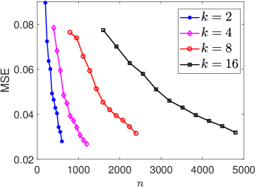
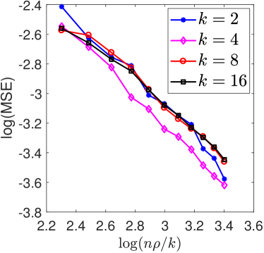
(a)	(b)

Figure 1: The MSE error of USVT estimator under stochastic block models for varying number of blocks $k$ and a fixed observation probability $\rho=0.1$. Panel (a): MSE versus the number of vertices $n$; Panel (b): The log of MSE versus $\log(n\rho/k)$. Each point represents the average of MSE over $20$ independent runs.

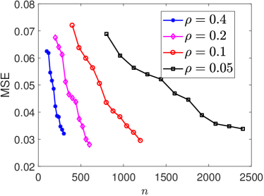
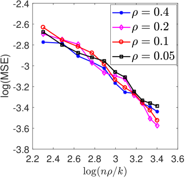
(a)	(b)

Figure 2: The MSE error of USVT estimator under stochastic block models for varying observation probabilities and a fixed number of blocks $k=4$. Panel (a): MSE versus the number of vertices $n$; Panel (b): The log of MSE versus $\log(n\rho/k)$. Each point represents the average of MSE over $30$ independent runs.

4.2 Translation invariant graphon

For some $a>0$, let $h:[-a,a]\to{\mathbb{R}}$ denote an even function, i.e., $h(x)=h(-x)$. Let us extends its domain to the real line by the periodic extension such that $h(x+2ka)=h(x)$ for all $x\in[-a,a]$ and integers $k\in{\mathbb{Z}}.$ By construction $h$ has a period $2a$. Using this function, we can define a translation-invariant graphon on the product space $[-a,a]\times[-a,a]$ via $f(x,y)=h(x-y)$. Since $h$ is even, it follows that $f$ is symmetric. Then the integral operator ${\mathcal{T}}$ defined in (11) reduces to

$$\left({\mathcal{T}}g\right)(x)=\frac{1}{2a}\int_{-a}^{a}h(x-y)g(y){\rm d}y=\frac{1}{2a}\left(h\ast g\right)(x),\quad\forall x\in[-a,a],$$

where $\ast$ denotes the convolution. Hence, we can explicitly determine the eigenvalues of ${\mathcal{T}}$ via Fourier analysis. In particular, suppose that $h$ has the following Fourier series expansion:

$$h(x)=\sum_{k=-\infty}^{\infty}\widehat{h}[k]e^{j\pi kx/a},\quad\widehat{h}[k]=\frac{1}{2a}\int_{-a}^{a}h(x)e^{-j\pi kx/a}{\rm d}x.$$

where throughout this section $j$ denotes the imaginary part such that $j^{2}=-1$, and $\widehat{h}[k]$ are the Fourier coefficients. Since $h$ is even, it follows that $\widehat{h}[k]$’s are real and $\widehat{h}[k]=\widehat{h}[-k]$. Fourier analysis entails a one-to-one correspondence between eigenvalues of ${\mathcal{T}}$ and Fourier coefficients of $h$: $\lambda_{k}({\mathcal{T}})=\widehat{h}[k]$.

We specify $h:[-1,1]\to{\mathbb{R}}$ as $h(x)=|x|$ and simulate the graphon model with $f(x,y)=h(x-y)$ for $x,y\in[-1,1]$ and the underlying measure $\mu$ being uniform over $[-1,1]$. Since $h(x)=|x|$, the Fourier coefficients can be explicitly computed as $\lambda_{k}({\mathcal{T}})=\widehat{h}[k]=2\sin^{2}(\pi k/2)/(\pi^{2}k^{2})$ with eigenfunctions given by $\{\cos(\pi kx)\}_{k=0}^{\infty}$ and $\sin(\pi kx)\}_{k=1}^{\infty}$. It follows from Theorem 5 that the eigenvalues of $M$ satisfy

$$\frac{1}{n^{2}}\sum_{i\geq r+1}\mathbb{E}\left[\lambda_{i}^{2}(M)\right]\leq O(n^{-1})+O(r^{-3})$$

uniformly over all integers $r\geq 0.$ Therefore, our theory predicts that the MSE of USVT converges to zero at least in a rate of $(n\rho)^{-3/4}$. The simulation results for varying observation probabilities are depicted in Fig. 3. Panel (a) shows the MSE converges to $0$ as the number of vertices $n$ increases. In Panel (b), we rescale the $x$-axis to $\log(n\rho)$ and the $y$-axis to the log of MSE. The curves for different $\rho$ align well with each other after the rescaling and decrease linearly with a slope of approximately $0.8$, which is close to $3/4$ as predicted by our theory.

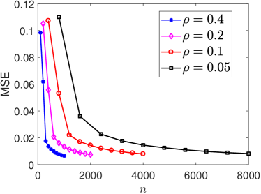
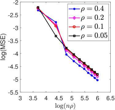
(a)	(b)

Figure 3: The MSE error of USVT estimator under the translation invariant graphon $f(x,y)=|x-y|$. Panel (a): MSE versus the number of vertices $n$; Panel (b): The log of MSE versus $\log(n\rho).$ Each point represents the average of MSE over $10$ independent runs.

4.3 Sobolev graphon

In this section, we simulate the graphon model with ${\mathcal{X}}=[0,1]$ and $\mu$ being the uniform measure and $f(x,y)=\min\{x,y\}$. Then $\nabla_{x}f(x,y)={\mathbf{1}_{\left\{{x\leq y}\right\}}}$ and $\nabla_{y}f(x,y)={\mathbf{1}_{\left\{{y\leq x}\right\}}}$. Moreover, $|f(x,y)-f(x^{\prime},y^{\prime})|\leq|x-x^{\prime}|+|y-y^{\prime}|$. However, the second-order weak derivatives of $f$ do not exist. Therefore, $f$ is Sobolev smooth with $\alpha=1.$ In this case, one can get a bound on the eigenvalue decay rate tighter than Proposition 1 by directly computing $\lambda_{n}({\mathcal{T}})$ and invoking Theorem 5. Note that

$$\left({\mathcal{T}}g\right)(x)=\int_{0}^{1}\min\{x,y\}g(y){\rm d}y=\int_{0}^{x}yg(y){\rm d}y+x\int_{x}^{1}g(y){\rm d}y.$$

Suppose $\phi$ is an eigenfunction of ${\mathcal{T}}$ with eigenvalue $\lambda$. Then

$$\int_{0}^{x}y\phi(y){\rm d}y+x\int_{x}^{1}\phi(y){\rm d}y=\lambda\phi(x).$$

It follows that $\phi(0)=1$ and $\lambda\phi^{\prime}(x)=\int_{x}^{1}\phi(y){\rm d}y$. It further implies that $\phi^{\prime}(1)=0$ and $\lambda\phi^{\prime\prime}+\phi=0.$ Therefore, the eigenfunction and eigenvalue pairs are given by

$$\phi_{k}(x)=\sin\frac{(2k-1)\pi x}{2},\text{ and }\lambda_{k}({\mathcal{T}})=\left(\frac{2}{(2k-1)\pi}\right)^{2}.$$

It follows from Theorem 5 that the eigenvalues of $M$ satisfy

$$\frac{1}{n^{2}}\sum_{i\geq r+1}\mathbb{E}\left[\lambda_{i}^{2}(M)\right]\leq O(n^{-1})+O(r^{-3})$$

uniformly over all integers $r\geq 0$. Therefore, our theory predicts that the MSE of USVT converges to zero in a rate of $(n\rho)^{-3/4}$. The simulation results for varying observation probabilities are depicted in Fig. 3. The curves in Panel (b) for different $\rho$ align well with each other after the rescaling and decrease linearly with a slope of approximately $0.7$, which is close to $3/4$ as predicted by our theory.

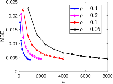
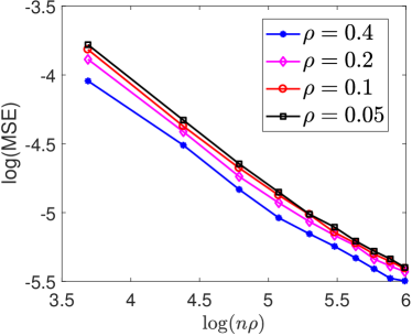
(a)	(b)

Figure 4: The MSE error of USVT estimator under the first-order sobolev graphon $f(x,y)=\min\{x,y\}.$ Panel (a): MSE versus the number of vertices $n$; Panel (b): The log of MSE versus $\log(n\rho).$ Each point represents the average of MSE over $10$ independent runs.

5 Conclusions and future work

In this paper, we establish upper bounds to the graphon estimation error of the universal singular value thresholding algorithm in the relatively sparse regime where the average vertex degree is at least logarithmic in $n.$ In both the stochastic block model setting and the smooth graphon setting, we show that the estimation error of USVT converges to $0$ as $n\to\infty$. Moreover, when graphon function $f$ belongs to Hölder or Sobolev space with smootheness index $\alpha$, we show that the rate of convergence is at most $(n\rho)^{-2\alpha/(2\alpha+d)}$, approaching the minimax optimal rate $\log(n\rho)/(n\rho)$ proved in the literature for $d=1$, as $f$ gest smoother. Furthermore, when $f$ is analytic with infintely many times differentiability, we show the rate of convergence is at most $\log^{d}(n\rho)/(n\rho)$.

A future direction important in both theory and practice is to develop computationally efficient graphon estimation procedures in networks with bounded average degrees and characterize the rate of convergence of the estimation error. Another fundamental and open question is whether the minimax optimal rate can be achieved in polynomial-time. For stochastic block models with $k$ blocks, we observe a multiplicative gap of $k/\log k$ between the rate of convergence of USVT and the minimax optimal rate. For Hölder or Sobolev smooth graphons with smoothness index $\alpha$ and the latent feature space of dimension $d=1$, we observe a multiplicative gap of $(n\rho)^{1/(2\alpha+1)}/\log(n\rho)$ between the rate of convergence of USVT and the minimax optimal rate. The minimax optimal rates are unknown for Hölder or Sobolev smooth graphons with $d>1$ and analytic graphons with $d\geq 1.$

Appendix A Proof of (10)

It has been shown in [28, 19] that the minimax optimal error rate of estimating $\alpha$-Hölder smooth graphon is given by:

$$\inf_{\widehat{M}}\sup_{f\in{\mathcal{H}}(\alpha,L)}\sup_{\mu\in{\mathcal{P}}[0,1]}\textup{MSE}(\widehat{M})\asymp\min_{1\leq k\leq n}\left\{\frac{k^{2}}{n^{2}\rho}+\frac{\log k}{n\rho}+k^{-2(\alpha\wedge 1)}\right\}\wedge 1.$$

Next, we solve the above minimization problem over $k$ by dividing the analysis into four cases. Combining all four cases completes the proof.

Case 1: $\log(n\rho)\geq\alpha\log n+(\alpha+1)\log\log n$. In this case, we must have $\alpha\leq 1$. We set $k=\lfloor(n^{2}\rho)^{1/(2\alpha+2)}\rfloor$ and get that

$$\min_{1\leq k\leq n}\left\{\frac{k^{2}}{n^{2}\rho}+\frac{\log k}{n\rho}+k^{-2(\alpha\wedge 1)}\right\} \leq 2(n^{2}\rho)^{-\alpha/(\alpha+1)}+\frac{1}{2\alpha+2}\frac{\log(n^{2}\rho)}{n\rho}$$

$$\leq 2(n^{2}\rho)^{-\alpha/(\alpha+1)}+\frac{\log n}{n\rho}$$

$$\leq 3(n^{2}\rho)^{-\alpha/(\alpha+1)}.$$

where the last inequality holds because $\log(n\rho)\geq\alpha\log n+(\alpha+1)\log\log n$ is equivalent to $(n^{2}\rho)^{-\alpha/(\alpha+1)}\geq\log n/(n\rho).$

On the contrary,

$$\min_{1\leq k\leq n}\left\{\frac{k^{2}}{n^{2}\rho}+\frac{\log k}{n\rho}+k^{-2(\alpha\wedge 1)}\right\}\geq\min_{1\leq k\leq n}\left\{\frac{k^{2}}{n^{2}\rho}+k^{-2\alpha}\right\}\geq(n^{2}\rho)^{-\alpha/(\alpha+1)}.$$

Case 2: $\alpha\log n\leq\log(n\rho)\leq\alpha\log n+(\alpha+1)\log\log n$. In this case, we still have $\alpha\leq 1$ and set $k=\lfloor(n^{2}\rho)^{1/(2\alpha+2)}\rfloor$. We get that

$$\min_{1\leq k\leq n}\left\{\frac{k^{2}}{n^{2}\rho}+\frac{\log k}{n\rho}+k^{-2(\alpha\wedge 1)}\right\} \leq 2(n^{2}\rho)^{-\alpha/(\alpha+1)}+\frac{\log n}{n\rho}$$

$$\leq\frac{3\log n}{n\rho}\leq\frac{3\log(n\rho)}{\alpha n\rho},$$

where in the last two inequalities we used the assumption that $\alpha\log n\leq\log(n\rho)\leq\alpha\log n+(\alpha+1)\log\log n$.

On the contrary,

$$\min_{1\leq k\leq n}\left\{\frac{k^{2}}{n^{2}\rho}+\frac{\log k}{n\rho}+k^{-2(\alpha\wedge 1)}\right\}\geq\min_{1\leq k\leq n}\left\{\frac{\log k}{n\rho}+k^{-2\alpha}\right\}\geq\frac{\log(n\rho)}{4\alpha n\rho}.$$

Case 3: $\omega(1)=\log(n\rho)\leq\alpha\log n$. In this case, we set

$$k=\lfloor(n\rho)^{\frac{1}{2(\alpha\wedge 1)}}\rfloor$$

and get that

$$\min_{1\leq k\leq n}\left\{\frac{k^{2}}{n^{2}\rho}+\frac{\log k}{n\rho}+k^{-2(\alpha\wedge 1)}\right\}\leq\frac{\left(n\rho\right)^{\frac{1}{\alpha\wedge 1}}}{n^{2}\rho}+\frac{1}{2(\alpha\wedge 1)}\frac{\log(n\rho)}{n\rho}+\frac{1}{n\rho}\leq\frac{2}{n\rho}+\frac{1}{2(\alpha\wedge 1)}\frac{\log(n\rho)}{n\rho},$$

where the last inequality holds because $(n\rho)^{1/(\alpha\wedge 1)}\leq n$. The proof of the lower bound is similar to that in Case 2.

Case 4: $n\rho=O(1)$. In this case, we trivially have

$$\min_{1\leq k\leq n}\left\{\frac{k^{2}}{n^{2}\rho}+\frac{\log k}{n\rho}+k^{-2(\alpha\wedge 1)}\right\}\wedge 1\asymp 1.$$

References

- [1] E. Abbe and C. Sandon. Detection in the stochastic block model with multiple clusters: proof of the achievability conjectures, acyclic bp, and the information-computation gap. arXiv 1512.09080, Dec 2015.
- [2] E. M. Airoldi, T. B. Costa, and S. H. Chan. Stochastic blockmodel approximation of a graphon: Theory and consistent estimation. In Advances in Neural Information Processing Systems 26, pages 692–700, 2013.
- [3] A. S. Bandeira and R. van Handel. Sharp nonasymptotic bounds on the norm of random matrices with independent entries. arXiv 1408.6185, 2014.
- [4] J. Banks, C. Moore, , N. Verzelen, R. Vershynin, and J. Xu. Information-theoretic bounds and phase transitions in clustering, sparse PCA, and submatrix localization. arXiv 1607.05222, June 2016.
- [5] J. Banks, C. Moore, J. Neeman, and P. Netrapalli. Information-theoretic thresholds for community detection in sparse networks. In Proceedings of the 29th Conference on Learning Theory, COLT 2016, New York, NY, June 23-26 2016, pages 383–416, 2016.
- [6] P. J. Bickel and A. Chen. A nonparametric view of network models and newman–girvan and other modularities. Proceedings of the National Academy of Sciences, 106(50):21068–21073, 2009.
- [7] M. S. Birman and M. Z. Solomyak. Piecewise-polynomial approximations of functions of the classes . Mathematics of the USSR-Sbornik, 2(3):295, 1967.
- [8] M. S. Birman and M. Z. Solomyak. Estimates of singular numbers of integral operators. Russian Mathematical Surveys, 32(1):15, 1977.
- [9] C. Borgs, J. Chayes, and A. Smith. Private graphon estimation for sparse graphs. In Advances in Neural Information Processing Systems, pages 1369–1377, 2015.
- [10] C. Borgs, J. T. Chayes, L. Lovász, V. T. Sós, and K. Vesztergombi. Convergent sequences of dense graphs i: Subgraph frequencies, metric properties and testing. Advances in Mathematics, 219(6):1801–1851, 2008.
- [11] C. Borgs, J. T. Chayes, L. Lovász, V. T. Sós, and K. Vesztergombi. Convergent sequences of dense graphs ii. multiway cuts and statistical physics. Annals of Mathematics, 176(1):151–219, 2012.
- [12] D. Cai, N. Ackerman, and C. Freer. An iterative step-function estimator for graphons. arXiv preprint arXiv:1412.2129, 2014.
- [13] S. Chan and E. Airoldi. A consistent histogram estimator for exchangeable graph models. In Proceedings of the 31st International Conference on Machine Learning (ICML-14), pages 208–216, 2014.
- [14] S. Chatterjee. Matrix estimation by universal singular value thresholding. The Annals of Statistics, 43(1):177–214, 2015.
- [15] Y. Chen and J. Xu. Statistical-computational tradeoffs in planted problems and submatrix localization with a growing number of clusters and submatrices. In Proceedings of ICML 2014 (Also arXiv:1402.1267), Feb 2014.
- [16] J. Delgado and M. Ruzhansky. Schatten classes on compact manifolds: kernel conditions. Journal of Functional Analysis, 267(3):772–798, 2014.
- [17] P. Erdös and A. Rényi. On random graphs, I. Publicationes Mathematicae (Debrecen), 6:290–297, 1959.
- [18] U. Feige and E. Ofek. Spectral techniques applied to sparse random graphs. Random Struct. Algorithms, 27(2):251–275, Sept. 2005.
- [19] C. Gao, Y. Lu, Z. Ma, and H. H. Zhou. Optimal estimation and completion of matrices with biclustering structures. Journal of Machine Learning Research, 17(161):1–29, 2016.
- [20] C. Gao, Y. Lu, H. H. Zhou, et al. Rate-optimal graphon estimation. The Annals of Statistics, 43(6):2624–2652, 2015.
- [21] B. Hajek, Y. Wu, and J. Xu. Achieving exact cluster recovery threshold via semidefinite programming. IEEE Transactions on Information Theory, 62(5):2788–2797, May 2016. (arXiv 1412.6156 Nov. 2014).
- [22] B. Hajek, Y. Wu, and J. Xu. Semidefinite programs for exact recovery of a hidden community. In Proceedings of Conference on Learning Theory (COLT), pages 1051–1095, New York, NY, Jun 2016. arXiv:1602.06410.
- [23] M. S. Handcock, A. E. Raftery, and J. M. Tantrum. Model-based clustering for social networks. Journal of the Royal Statistical Society: Series A (Statistics in Society), 170(2):301–354, 2007.
- [24] P. D. Hoff, A. E. Raftery, and M. S. Handcock. Latent space approaches to social network analysis. Journal of the American Statistical Association, 97:1090+, December 2002.
- [25] P. W. Holland, K. B. Laskey, and S. Leinhardt. Stochastic blockmodels: First steps. Social Networks, 5(2):109–137, 1983.
- [26] T. Kato. Perturbation Theory for Linear Operators. Springer, Berlin, 1966.
- [27] O. Klopp et al. Rank penalized estimators for high-dimensional matrices. Electronic Journal of Statistics, 5:1161–1183, 2011.
- [28] O. Klopp, A. B. Tsybakov, and N. Verzelen. Oracle inequalities for network models and sparse graphon estimation. arXiv preprint arXiv:1507.04118, 2015.
- [29] O. Klopp and N. Verzelen. Optimal graphon estimation in cut distance. arXiv preprint arXiv:1703.05101, 2017.
- [30] V. Koltchinskii and E. Giné. Random matrix approximation of spectra of integral operators. Bernoulli, pages 113–167, 2000.
- [31] V. Koltchinskii, K. Lounici, A. B. Tsybakov, et al. Nuclear-norm penalization and optimal rates for noisy low-rank matrix completion. The Annals of Statistics, 39(5):2302–2329, 2011.
- [32] V. I. Koltchinskii. Asymptotics of spectral projections of some random matrices approximating integral operators. Progress in Probability, 1998.
- [33] H. Komatsu. A characterization of real analytic functions. Proceedings of the Japan Academy, 36(3):90–93, 1960.
- [34] H. König. Eigenvalue distribution of compact operators, volume 16. Birkhäuser, 2013.
- [35] I. G. Y. M. Krein. Introduction to the theory of linear nonselfadjoint operators in hilbert space. American Mathematical Society, 1965.
- [36] C. E. Lee and D. Shah. Unifying framework for crowd-sourcing via graphon estimation. arXiv preprint arXiv:1703.08085, 2017.
- [37] G. Leoni. A first course in Sobolev spaces, volume 105. American Mathematical Society Providence, RI, 2009.
- [38] G. Little and J. Reade. Eigenvalues of analytic kernels. SIAM journal on mathematical analysis, 15(1):133–136, 1984.
- [39] L. Lovász. Large networks and graph limits, volume 60. American Mathematical Society Providence, 2012.
- [40] L. Lovász and B. Szegedy. Limits of dense graph sequences. Journal of Combinatorial Theory, Series B, 96(6):933–957, 2006.
- [41] L. Massoulié and D. Tomozei. Distributed user profiling via spectral methods. Stochastic Systems, 4(1):1–43, 2014.
- [42] K. Miller, M. I. Jordan, and T. L. Griffiths. Nonparametric latent feature models for link prediction. In Advances in neural information processing systems, pages 1276–1284, 2009.
- [43] C. Moore. The computer science and physics of community detection: landscapes, phase transitions, and hardness. arXiv preprint arXiv:1702.00467, 2017.
- [44] M. Pensky. Dynamic network models and graphon estimation. arXiv preprint arXiv:1607.00673, 2016.
- [45] N. Shah, S. Balakrishnan, A. Guntuboyina, and M. Wainwright. Stochastically transitive models for pairwise comparisons: Statistical and computational issues. In International Conference on Machine Learning, pages 11–20, 2016.
- [46] D. Song, C. E. Lee, Y. Li, and D. Shah. Blind regression: Nonparametric regression for latent variable models via collaborative filtering. In Advances in Neural Information Processing Systems, pages 2155–2163, 2016.
- [47] A. B. Tsybakov. Introduction to Nonparametric Estimation. Springer Publishing Company, Incorporated, 1st edition, 2008.
- [48] U. von Luxburg, O. Bousquet, and M. Belkin. On the convergence of spectral clustering on random samples: the normalized case. NIPS, 2005.
- [49] P. J. Wolfe and S. C. Olhede. Nonparametric graphon estimation. arXiv preprint arXiv:1309.5936, 2013.
- [50] J. Xu, L. Massoulié, and M. Lelarge. Edge label inference in generalized stochastic block models: from spectral theory to impossibility results. In COLT, pages 903–920, 2014.
- [51] J. Yang, C. Han, and E. Airoldi. Nonparametric estimation and testing of exchangeable graph models. In Artificial Intelligence and Statistics, pages 1060–1067, 2014.
- [52] H. Yu, P. Braun, M. A. Yıldırım, I. Lemmens, K. Venkatesan, J. Sahalie, T. Hirozane-Kishikawa, F. Gebreab, N. Li, N. Simonis, et al. High-quality binary protein interaction map of the yeast interactome network. Science, 322(5898):104–110, 2008.
- [53] Y. Zhang, E. Levina, and J. Zhu. Estimating network edge probabilities by neighborhood smoothing. arXiv preprint arXiv:1509.08588, 2015.