Steady state detection for computational fluid dynamics

Abstract

Large parameter studies of fluid dynamic instabilities can crucially be simplified, if the user does not need to specify the simulation time. For this purpose, a steady state detection is implemented in the CFD library OpenFOAM. It terminates simulations automatically if characteristic measurements do not change over time, i.e. when saturation is reached. For that purpose, recent data is compared to previous one using two selectable methods. Both calculate a value used as steady state indicator. The first method performing a two sample Student’s t-test examines the difference between the means. Similarly, the second method utilises a two sample f-test checking for changes between the variances. Both methods are briefly described, compared and their specific area of application is discussed. Their usefulness is demonstrated with a simple exemplary test case.

1 Introduction

An instability arises when exceeding a certain critical threshold. It grows then exponentially until reaching a saturated state. In order to determine the characteristic properties of a fluid dynamic instability (as, e.g., growth rate, steady state velocity) transient numerical simulation is required. A priori, the time for reaching the saturated state is unknown. A steady state detection (SSD) or steady state identification system can determine when saturation is reached and switch off the simulation automatically. This saves space on the hard drive. More importantly, an SSD system can drastically reduce user interaction, because the simulation time does not need to be provided any more. That will be especially useful when doing large parameter studies, where the time to reach saturation depends on the parameter. An SSD is not only useful for simulating instabilities, but for all transient flow phenomena.

A reasonable SSD method must satisfy several requirements: firstly, it should not need any or very little user input. Secondly, it must be robust, i.e. the saturated state must be detected securely. Thirdly, it should be universal, i.e. different types of saturated states need be detected. Finally, the SSD should be computationally simple and easy to implement [1, 2].

Steady state detection is well established in process control. There, deviations from the steady state, i.e. from the steady process need to be detected. All common SSD methods use statistical approaches; the most popular is the one by Cao and Rhinehart [3]. For a short introduction to different methods, see [4, 5] and for a detailed overview [2].

All common methods analyse a moving window [6] of recent measurement data. It does not exist an universal rule for the length of this window [3]: a long one will lead to a delayed steady state detection, a short one will increase noise [4]. Applied to numerical simulation, the “measurement” data may be, e.g., the volume averaged velocity of each time step.

One simple way for SSD is performing a linear regression of the measurement data inside the window. If steady, the slope should ideally be zero. This can be verified easily with a t-test [3, 2]. Such a method is used by [7] while [8] uses the first derivative of a polynomial regression.

Another option is comparing the mean values of measurement data between two subsequent windows. If the means do not change, the steady state is reached. This hypothesis can easily be checked using a two sample t-test [3, 2] and is used e.g., by [9].

Alternatively, the standard deviations between two subsequent windows may be compared using an f-test. In a steady state, the relation of both should be one. A very similar approach consists in computing the standard deviation in one window only, but using two different ways of calculation. The hypothesis of a steady state is tested by an f-like statistics, the r-test [3]. For critical values for type I and II errors see [10, 11]. This is the most commonly used SSD method in process control [12, 4, 13, 14].

Finally, also a wavelet approach may be used for SSD [15, 5]. However, it is rather complex, and therefore not discussed in detail here.

2 Comparison of different SSD mechanisms

Steady state detection in numerical simulation is different to process control: typically, the “measurement” error in simulation is very small compared to reality. While process control aims in detecting a deviation of the steady process, we search the steady state itself.

A saturated flow can generally be classified into three different categories: firstly, it may be really steady, with ideally no fluctuations. Secondly, it may be periodically oscillating and thirdly turbulent. Detecting these different types of saturated states with one method will be challenging. Therefore, we focus in this article as a first step on real steady states only.

Table 1 illustrates how different tests fulfil the requirements to SSD described in the introduction. A linear regression test will work generally fine except for oscillating or turbulent flow. However, it is computationally expensive – a disadvantage which it has in common with the wavelet test. Anyway, the latter might be interesting for detecting unsteady saturated flows.

The t-test is robust, simple and universal. It may even be used for unsteady saturated flows. However, its application to oscillating flows is limited: the moving window must be large enough to include a full period. Further, an oscillating flow with changing amplitude might be detected as steady, as long as the mean does not change. This drawback can be compensated using an f-test. It will detect falling or rising oscillation periods. However, as it compares only standard deviations it can not detect changing means.

In many cases, a double t-test will be the optimal method for steady state detection. A composite f-t-test, which compares both, means and standard deviations, will be even safer in the sense of avoiding a false steady state detection.

Table 1: Requirements to steady state detection and performance of different SSD methods (+ means good, – bad).

criteria	linear regression	t-test	f-test	wavelet
robustness	?	+	–	?
universality	–	+	+	–
low user interaction	?	?	?	?
computationally simple	–	+	+	–

3 Theory and implementation

We will describe the double t-, f- and f-t-composite test in the following. All of them check the null hypothesis of a steady state. In a first step, the size of two consecutive moving windows needs to be defined. Often, the time step of the simulation is determined by the flow velocity using some kind of Courant Friedrich Levy number. It is therefore reasonable to use a fixed number of $n$ time steps to define the size of each moving window. The arithmetic mean of a property $x$ (e.g. volumetric averaged velocity) of the first and second window is defined as

$$\overline{x}_{1}=\frac{1}{n}\sum_{i=k-2n+1}^{k-n}x_{i}\qquad\text{and}\qquad\overline{x}_{2}=\frac{1}{n}\sum_{i=k-n+1}^{k}x_{i}$$ (1)

with $k$ denoting the current time step index. Similarly, the variances are

$$s_{1}^{2} =\frac{1}{n-1}\sum_{i=k-2n+1}^{k-n}\left(x_{i}-\overline{x}_{1}\right)^{2}\quad\text{and}$$ (2)

$$s_{2}^{2} =\frac{1}{n-1}\sum_{i=k-n+1}^{k}\left(x_{i}-\overline{x}_{2}\right)^{2}.$$ (3)

After the simulation has run through the first $2n$ time steps, the means and variances are computed using the old values of $\overline{x}$ and $s$ and the new data point $x_{k}$ as

$$\overline{x}_{1,k} =\overline{x}_{1,k-1}-\frac{x_{k-2n}-x_{k-n}}{n}$$ (4)

$$\overline{x}_{2,k} =\overline{x}_{2,k-1}-\frac{x_{k-n}-x_{k}}{n}$$ (5)

$$s_{1,k}^{2} =s_{1,k-1}^{2}-\frac{x_{k-2n}^{2}-x_{k-n}^{2}-n\cdot(\overline{x}_{1,k-1}^{2}-\overline{x}_{1,k}^{2})}{n-1}$$ (6)

$$s_{2,k}^{2} =s_{2,k-1}^{2}-\frac{x_{k-n}^{2}-x_{k}^{2}-n\cdot(\overline{x}_{2,k-1}^{2}-\overline{x}_{2,k}^{2})}{n-1}.$$ (7)

Please note that the point $x_{k-2n}$ is just outside of both windows. This procedure is more efficient than recalculating means and variances from all time steps [6].

The t-test compares the means between two consecutive moving windows. In order to obtain a dimensionless value, the mean is divided by the square root of the variances. The test statistics is

$$T=\frac{|\overline{x}_{2}-\overline{x}_{1}|}{\sqrt{s_{1}^{2}+s_{2}^{2}}}\sqrt{n}.$$ (8)

For a perfectly steady state, $T$ will be zero. However, the variances will be zero, too. In that case, $T$ will be infinite. To avoid such kind of problems, we add an artificial error of 1 % to the data points when calculating the variances.

The f-test compares the variances between the two sampling windows. The test statistics is defined as

$$F=\frac{\text{max}(s_{1}^{2},s_{2}^{2})}{\text{min}(s_{1}^{2},s_{2}^{2})}.$$ (9)

At steady state, $F$ will ideally be one. Again, $\sigma^{2}$ should not get zero and therefore a 1 % artificial error is added during it’s calculation.

The combined f-t test checks first the f- and thereafter the t-test. Only if both detect a steady state, the simulation ends. Critical values for $T$ and $F$ can be given by statistical approaches [16, 11] or may be chosen empirically after doing a single test simulation as described in the following section. Further, an appropriate number of samples ($n$) must be selected.

4 OpenFOAM Testcase

We use the Tayler instability (TI) [17] as exemplary test case for the developed steady state detection system. When an electrical current flows through a liquid conductor, the resulting Lorentz force is always directed to the centre of the conductor. This configuration is unstable if a certain critical current is exceeded. The TI is not only discussed in context of a possible explanation of the 11-years solar cycle [18, 19, 20, 21, 22] but also as some upper limit for the design of liquid metal batteries [23, 24, 25]. The latter are proposed as a cheap grid-scale energy storage for fluctuating renewable energies [26].

We simulate the TI in a cylindrical liquid metal conductor of diameter $d=0.1$ m, height $h=0.125$ m, density $\rho=600\,$kg/m³, kinematic viscosity $\nu=2.5\cdot 10^{-7}$ m²/s and electrical conductivity $\sigma=3.2\cdot 10^{6}$ S/m. Figure 1a shows the general flow structure and figure 1b the volumetric averaged velocity over time for an applied electric current of $I=4$ kA. The exponential growth phase and the steady state can be observed very well. We apply the statistical tests using the volume averaged velocity.

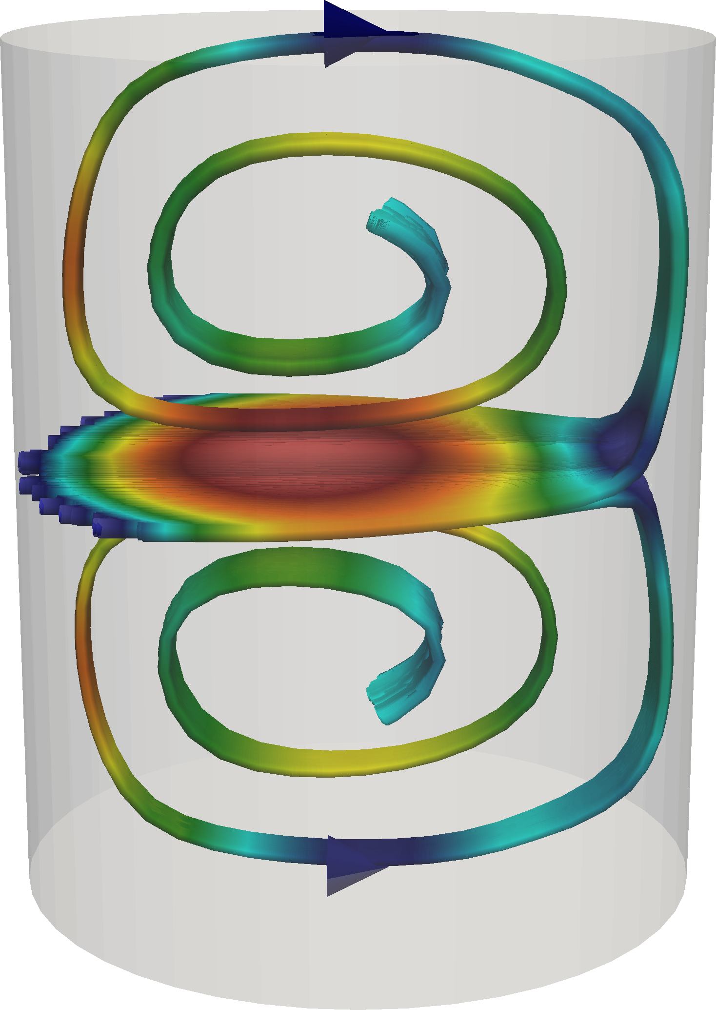
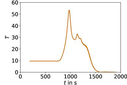
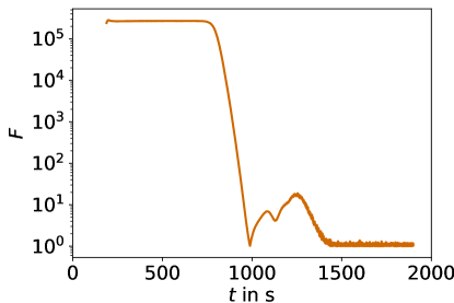
Figure 1: General flow structure of the Tayler instability in a cylindrical vessel (a), volume averages velocity over time for $I=4$ kA (b) and test statistics over time for the t- (c) and f-test (d).

It can be well observed in fig. 1c that the test statistics of the t-test goes to a value close to zero only in the saturated state. Similarly, the test statistics of the f-test (fig. 1d) reaches a value close to one. However, the latter is less reliable, as it detects already a false steady state during the growth of the instability.

Many test runs revealed that $F$ depends only slightly and $T$ not at all on the applied current of the Tayler instability. However, both statistics depend strongly on the number of samples $n$, i.e. on the size of the moving window. While the t-test works already well with only ten sampling values, the f-test needs at least 100 samples. Such a large number of samples allows for a better distinction between a growing and steady flow. Unfortunately, also the steady state value of the statistics $T$ and $F$ depends on the number of samples. For the particular case of the Tayler instability we recommend $F_{\text{cr}}=1.6$ with $n=100$ and $T_{\text{cr}}=n\cdot 5\cdot 10^{-4}$ with $n\geq 10$. A steady state is likely reached, when $T$ and $F$ fall below of $T_{\text{cr}}$ and $F_{\text{cr}}$. The probably best way of adapting the SSD to other instabilities is doing a test simulation with a coarse grid. Reasonable critical values for $T$ and $F$ can easily be determined using a simple python script.

5 Summary and outlook

We have discussed where and why a steady state detection (SSD) system can be beneficial in computational fluid dynamics. We have further specified the requirements for a suitable method. After categorising saturated flow states into steady, oscillating and turbulent we have focused our attention to purely steady states, only. We further compared different statistical SSD methods and selected a double f- and t-test as the most promising approaches. The tests compare the means and variances of two consecutive moving windows of simulation data. A steady state is detected when they do not change any more. We have further demonstrated the usefulness of the developed SSD system using the Tayler instability as exemplary case. We have shown, that the proper selection of the number of sample points $n$ and the critical value of the test-statistics $F_{\text{cr}}$ and $T\text{cr}$ is the most challenging part. We have provided typical values of all three variables.

In a next step, general rules for selecting $n$, $F_{\text{cr}}$ and $T_{\text{cr}}$ shall be developed. The SSD library will be extensively tested and continuously improved. In a first step it is planned to use it for other instabilities, as, e.g., Rayleigh-Bénard convection [27, 28] and the metal pad roll instability in liquid metal batteries [29, 30, 31]. On the long run, the SSD system is planned to be extended to cope with oscillating and turbulent saturated flows.

References

References

- [1] V. Padmanabhan, R. R. Rhinehart, A novel termination criterion for optimization, in: American Control Conference, 2005. Proceedings of the 2005, IEEE, 2005, pp. 2281–2286.
- [2] R. R. Rhinehart, Automated steady and transient state identification in noisy processes, in: American Control Conference (ACC), 2013, IEEE, 2013, pp. 4477–4493.
- [3] S. Cao, R. Rhinehart, An efficient method for on-line identification of steady state, J. Process Control 5 (6) (1995) 363–374.
- [4] S. A. Bhat, D. N. Saraf, Steady-State Identification, Gross Error Detection, and Data Reconciliation for Industrial Process Units, Ind. Eng. Chem. Res. 43 (15) (2004) 4323–4336.
- [5] D. Al Gobaisi, Encyclopedia of Desalination and Water Resources, EOLSS Publishers, Oxford, UK, 2000.
- [6] M. Kim, S. H. Yoon, P. A. Domanski, W. Vance Payne, Design of a steady-state detector for fault detection and diagnosis of a residential air conditioner, Int. J. Refrig. 31 (5) (2008) 790–799.
- [7] J. Wu, Y. Chen, S. Zhou, X. Li, Online Steady-State Detection for Process Control Using Multiple Change-Point Models and Particle Filters, IEEE T. Autom. Sci. Eng. 13 (2) (2016) 688–700.
- [8] G. A. Le Roux, B. F. Santoro, F. F. Sotelo, M. Teissier, X. Joulia, Improving steady-state identification, in: Comput. Aided Chem. Eng., Vol. 25, Elsevier, 2008, pp. 459–464.
- [9] J. D. Kelly, J. D. Hedengren, A steady-state detection (SSD) algorithm to detect non-stationary drifts in processes, J. Process Control 23 (3) (2013) 326–331.
- [10] S. Cao, R. R. Rhinehart, Critical values for a steady-state identifier, J. Process Control 7 (2) (1997) 149–152.
- [11] N. A. Shrowti, K. P. Vilankar, R. R. Rhinehart, Type-II critical values for a steady-state identifier, J. Process Control 20 (7) (2010) 885–890.
- [12] Y. Yao, C. Zhao, F. Gao, Batch-to-Batch Steady State Identification Based on Variable Correlation and Mahalanobis Distance, Ind. Eng. Chem. Res. 48 (24) (2009) 11060–11070.
- [13] P. R. Brown, R. R. Rhinehart, Demonstration of a method for automated steady-state identification in multivariable systems, Hydrocarbon process. 79 (9) (2000) 79–83.
- [14] B.-L. Huang, Y. Yao, Automatic steady state identification for batch processes by nonparametric signal decomposition and statistical hypothesis test, Chemometrics Intell. Lab. Sys. 138 (2014) 84–96.
- [15] T. Jiang, B. Chen, X. He, P. Stuart, Application of steady-state detection method based on wavelet transform, Comput. Chem. Eng. 27 (4) (2003) 569–578.
- [16] S. Cao, Statistically based techniques for process control applications, Ph.D. thesis, Texas Tech University (1996).
- [17] Y. V. Vandakurov, Theory for the stability of a star with a toroidal magnetic field, Astron. Zh+. 49 (2) (1972) 324 – 333.
- [18] A. Bonanno, A. Brandenburg, F. D. Sordo, D. Mitra, Breakdown of chiral symmetry during saturation of the Tayler instability, Phys. Rev. E 86 (016313).
- [19] M. Seilmayer, F. Stefani, T. Gundrum, T. Weier, G. Gerbeth, M. Gellert, G. Rüdiger, Experimental Evidence for a Transient Tayler Instability in a Cylindrical Liquid-Metal Column, Phys. Rev. Lett. 108 (244501).
- [20] N. Weber, V. Galindo, F. Stefani, T. Weier, The Tayler instability at low magnetic Prandtl numbers: Between chiral symmetry breaking and helicity oscillations, New Journal of Physics 17 (11) (2015) 113013.
- [21] F. Stefani, A. Giesecke, N. Weber, T. Weier, Synchronized Helicity Oscillations: A Link Between Planetary Tides and the Solar Cycle?, Solar Physics 291 (8) (2016) 2197–2212.
- [22] F. Stefani, V. Galindo, A. Giesecke, N. Weber, T. Weier, The Tayler instability at low magnetic Prandtl numbers: Chiral symmetry breaking and synchronizable helicity oscillations, Magnetohydrodynamics 53 (1) (2017) 169–178.
- [23] F. Stefani, T. Weier, T. Gundrum, G. Gerbeth, How to circumvent the size limitation of liquid metal batteries due to the Tayler instability, Energy Conversion and Management 52 (2011) 2982–2986.
- [24] W. Herreman, C. Nore, L. Cappanera, J.-L. Guermond, Tayler instability in liquid metal columns and liquid metal batteries, J. Fluid Mech. 771 (2015) 79–114.
- [25] T. Weier, A. Bund, W. El-Mofid, G. M. Horstmann, C.-C. Lalau, S. Landgraf, M. Nimtz, M. Starace, F. Stefani, N. Weber, Liquid metal batteries - materials selection and fluid dynamics, IOP Conf. Ser.: Mater. Sci. Eng. 228 (012013).
- [26] H. Kim, D. A. Boysen, J. M. Newhouse, B. L. Spatocco, B. Chung, P. J. Burke, D. J. Bradwell, K. Jiang, A. A. Tomaszowska, K. Wang, W. Wei, L. A. Ortiz, S. A. Barriga, S. M. Poizeau, D. R. Sadoway, Liquid Metal Batteries: Past, Present, and Future, Chemical Reviews 113 (3) (2013) 2075–2099. doi:10.1021/cr300205k.
- [27] Y. Shen, O. Zikanov, Thermal convection in a liquid metal battery, Theor. Comp. Fluid Dyn. 30 (4) (2016) 275–294.
- [28] T. Köllner, T. Boeck, J. Schumacher, Thermal Rayleigh-Marangoni convection in a three-layer liquid-metal-battery model, Phys. Rev. E 95 (053114).
- [29] O. Zikanov, Metal pad instabilities in liquid metal batteries, Physical Review E 92 (063021).
- [30] N. Weber, P. Beckstein, V. Galindo, W. Herreman, C. Nore, F. Stefani, T. Weier, Metal pad roll instability in liquid metal batteries, Magnetohydrodynamics 53 (1) (2017) 129–140.
- [31] G. M. Horstmann, N. Weber, T. Weier, Coupling and stability of interfacial waves in liquid metal batteries, arXiv:1708.02159.