Attractors in complex networks

Alexandre A. P. Rodrigues
Centro de Matemática da Universidade do Porto
and Faculdade de Ciências da Universidade do Porto
Rua do Campo Alegre 687, 4169–007 Porto, Portugal
Centro de Matemática da Universidade do Porto
and Faculdade de Ciências da Universidade do Porto

Rua do Campo Alegre 687, 4169–007 Porto, Portugal
alexandre.rodrigues@fc.up.pt
Abstract.

In the framework of the generalized Lotka Volterra model, solutions representing multispecies sequencial competition can be predictable with high probability. In this paper, we show that it occurs because the corresponding “heteroclinic channel” forms part of an attractor. We prove that, generically, in an attracting heteroclinic network involving a finite number of hyperbolic and non-resonant saddle-equilibria whose linearization has only real eigenvalues, the connections corresponding to the most positive expanding eigenvalues form a part of an attractor (observable in numerical simulations).

Key words and phrases:
Generalized Lotka Volterra model, Heteroclinic networks, Real eigenvalues, Attracting subnetwork, Essential asymptotic stability.
2010 Mathematics Subject Classification:
Primary: 34D23; Secondary: 34C37, 34D05, 34D20, 34D45.

Heteroclinic networks are much studied because they organise dynamics in which saddle-type equilibria are visible. Heteroclinic networks for differential equations can be accompanied by complicated nearby dynamics. Apart from topological descriptions of this complicated dynamics, a relevant question is the fate of typical, say for a full Lebesgue measure of initial conditions. This question has not always attracted appropriate attention. Asymptotic stability is well understood for a large class of heteroclinic cycles in the symmetric context. However, in many cases this is not satisfactory, because a Lyapunov unstable heteroclinic cycle may attract a set of large measure of initial states and may be observable in numerical simulations.

In the context of the generalized Lotka-Volterra system, the authors of [1, 27] studied heteroclinic networks whose linearization at the equilibria has only real eigenvalues. They claim that there is a preference of the system to evolve in the strongest direction with and without the influence of noise. Rigorous results about the ω𝜔\omega-limit sets for these networks are going to be needed in the very near future to discuss the stability of networks that appear in the context of winnerless competition and synchronization into clusters that appear in several biological systems.

In the present paper, motivated by partial results in [3] and supported by numerical simulations of [1, 27], we show that, within a heteroclinic network involving hyperbolic equilibria whose linearization has only real eigenvalues, generically the connections corresponding to the most positive expanding eigenvalues form a part of an attractor.

1. Introduction

Heteroclinic cycles are flow-invariant sets consisting of finitely many equilibria and trajectories connecting them in a cyclic fashion. They appear in several applications and are useful to the study of intermittent dynamics: a trajectory near a heteroclinic cycle will spend a long time in a neighbourhood of an equilibrium, before rapidly switching along a connection towards another equilibrium, where it stays again for a long period of time. Such behaviour is displayed, for example, by the geomagnetic field: its fast, unpredictable reversals of polarity are followed by long periods in a stationary mode. Many authors claim the presence of heteroclinic networks in the equations that describe geodynamic processes – see [25, 29] and references therein.

Another example occurs in population dynamics and has been treated in [1, 13]: as a model for competition between three or more species, Lotka-Volterra equations can possess attracting heteroclinic networks between equilibria in which there is only one winner. It seems for some time as if a unique species wins the competition and all others become extinct, before its density suddenly drops and its dominant state is taken by another species.

With dos Reis [9] and Guckenheimer and Holmes [10], it has been discovered that heteroclinic cycles and networks may be structurally stable in an equivariant context. Subsequently, their study gained importance. Placing the connections in flow-invariant subspaces, where they are of saddle-sink type, and restricting to perturbations that respect these symmetries, heteroclinic cycles becomes persistent invariant sets: if the invariant subspaces are not destroyed under small smooth perturbations, the cycle persists. In [15, 21], the authors give a comprehensive overview of early results on robust heteroclinic cycles.

The discovery of robustness ignited an interest on heteroclinic cycles in the nineties. Necessary and sufficient conditions for asymptotic stability of different types of cycles were derived in [22, 23]. However, being more complex in structure than a single hyperbolic equilibrium, heteroclinic cycles exhibit more complex stability features than the Lyapunov dichotomy asymptotic stability vs instability, in the sense that everything except for a set of zero Lebesgue measure might remain or leave a small neighbourhood of the cycle.

In [24], Melbourne presents a paradigmatic example of a cycle that is a non-asymptotically stable attractor: it attracts a set of positive Lebesgue measure of initial conditions, which is not a full neighbourhood of the cycle. The phenomenon becomes more surprising when several cycles are joined together to form a heteroclinic network. A cycle belonging to a network has at least one positive transverse eigenvalue and therefore cannot be asymptotically stable. However, in many cases, a dominant cycle may be “more stable” than the others in the sense that it may be the ω𝜔\omega-limit set of a large set (in terms of measure) of initial conditions in a neighbourhood of the network, even though the other cycles may attract infinitely many solutions. Brannath [5] provides simple examples of these networks on simplices, where a single cycle attracts a large set of initial conditions.

In [1, 27], the authors predict the behaviour of complex multi-agent systems, based on the Winnerless Competition Principle that induces robust dynamics in complex heteroclinic networks. See also [16]. Motivated by [17] and [1, 27], we may ask:

  1. (1)

    What are the limit sets of the network? According to [26], are they likely limit sets?

  2. (2)

    In the case of a stable heteroclinic network which is a union of the one-dimensional connections there are only a finite number of possible ω𝜔\omega-limit sets?

For general (non-symmetric) attracting heteroclinic networks, we expect the presence of essentially asymptotically stable subnetworks. More precisely, if ΓΓ\Gamma is an attracting heteroclinic network involving a finite number of equilibria with only real eigenvalues, then the connections corresponding to the most positive expanding eigenvalues of the linearization determine a possibly smaller attractor.

Key ideas of the proof

The key steps of this paper are a combination of the following ideas:

  • start with an attracting heteroclinic network whose linearization at the hyperbolic equilibria has real and non-resonant eigenvalues;

  • at each equilibrium point, its strong unstable manifold corresponds to a heteroclinic connection to the next equilibrium point;

  • in the same spirit of Deng’s Strong Lambda Lemma, we show that, near each equilibrium, the set of initial points that follow the strong unstable manifold is (locally) the complement of a wedge and thus has asymptotically full Lebesgue measure;

  • the complement of wedges are generically send (under the transition map) into the complement of other wedges with the same property. This process can be repeated ad infinitum.

Framework of the paper

The goal of this paper is to prove that, within a heteroclinic network whose nodes are hyperbolic equilibria whose linearization has only real eigenvalues, generically the connections corresponding to the most positive expanding eigenvalues form a part of an attractor (possibly not unique). The main result is stated in Section 3, after collecting relevant notions in Section 2. We also distinguish between various kinds of stability that have been developed along the last two decades.

Linearization techniques are used in Section 4 to construct a local transition map around the equilibria and also a return map around the cycle. This section deals with the geometrical structures which allow us to get an understanding of the dynamics. The proof of the main result is done in Section 5.

Throughout this paper, we have endeavoured to make a self contained exposition bringing together all definitions and topics related to the proofs. We have stated short lemmas and we have drawn illustrative figures to make the paper easily readable.

2. Preliminaries

In this section, we present and discuss some definitions which will be useful throughout the article. Let n,N𝐍𝑛𝑁𝐍n,N\in{\rm\bf N} where n4𝑛4n\geq 4, and G𝐺G is a compact region of 𝐑nsuperscript𝐑𝑛{\rm\bf R}^{n}. We consider a system of ordinary differential equations

(1) x˙=f(x),xG𝐑nformulae-sequence˙𝑥𝑓𝑥𝑥𝐺superscript𝐑𝑛\dot{x}=f(x),\qquad x\in G\subset{\rm\bf R}^{n}

where the vector field f:GG:𝑓𝐺𝐺f:G\rightarrow G is C2superscript𝐶2C^{2} with flow given by the unique solution x(t)φ(t,x0)G𝐑nmaps-to𝑥𝑡𝜑𝑡subscript𝑥0𝐺superscript𝐑𝑛x(t)\mapsto\varphi(t,x_{0})\in G\subset{\rm\bf R}^{n}. For xG𝑥𝐺x\in G, let us introduce the following norm in the set of vector fields:

fC1=supxG(f+fx),subscriptnorm𝑓superscript𝐶1subscriptsupremum𝑥𝐺norm𝑓norm𝑓𝑥||f||_{C^{1}}=\sup_{x\in G}\left(||f||+\left\|\frac{\partial f}{\partial x}\right\|\right),

where ||.||||.|| represents the norm of the maximum in 𝐑nsuperscript𝐑𝑛{\rm\bf R}^{n}. Endowed with this norm, the set of vector fields becomes a Banach space, denoted by 𝒳𝒳\mathcal{X}. A δ𝛿\delta-neighbourhood of the vector field f𝒳𝑓𝒳{f}\in\mathcal{X} is the set of all vector fields f~𝒳~𝑓𝒳\tilde{f}\in\mathcal{X} satisfying f~f<δ.norm~𝑓𝑓𝛿\left\|\tilde{f}-f\right\|<\delta.

2.1. Heteroclinic terminology

We start this subsection with a definition of heteroclinic cycle and network that suffices to our purposes.

Given two equilibria p1subscript𝑝1p_{1} and p2subscript𝑝2p_{2}, a heteroclinic connection from p1subscript𝑝1p_{1} to p2subscript𝑝2p_{2}, denoted [p1p2]delimited-[]subscript𝑝1subscript𝑝2[p_{1}\rightarrow p_{2}], is a connected flow-invariant manifold contained in Wu(p1)Ws(p2)superscript𝑊𝑢subscript𝑝1superscript𝑊𝑠subscript𝑝2W^{u}(p_{1})\cap W^{s}(p_{2}), where Ws(p)superscript𝑊𝑠𝑝W^{s}(p) and Wu(p)superscript𝑊𝑢𝑝W^{u}(p) refer to the stable and unstable manifolds of the hyperbolic equilibrium p𝑝p, respectively. The dimension of the unstable manifold of an equilibrium p𝑝p will be called the Morse index of p𝑝p. Throughout this work, we assume that the connections are one-dimensional.

Let 𝒮={pj:j{1,,N}}𝒮conditional-setsubscript𝑝𝑗𝑗1𝑁\mathcal{S=}\{p_{j}:j\in\{1,\ldots,N\}\} be a finite ordered set of equilibria. We say that there is a heteroclinic cycle associated with 𝒮𝒮\mathcal{S} if

j{1,,N},Wu(pj)Ws(pj+1)(modN).formulae-sequencefor-all𝑗1𝑁superscript𝑊𝑢subscript𝑝𝑗superscript𝑊𝑠subscript𝑝𝑗1annotatedpmod𝑁\forall j\in\{1,\ldots,N\},W^{u}(p_{j})\cap W^{s}(p_{j+1})\neq\emptyset\pmod{N}.

A heteroclinic network is a connected union of heteroclinic cycles. Hereafter, all equilibria (also called by nodes) will be hyperbolic. Depending on the geometry of their eigendirections, the eigenvalues of df𝑑𝑓df at the equilibria may be classified into four types: radial, contracting, expanding and transverse. We adress the reader to [22] for this classification.

2.2. Notions of Stability

In order to gain a broader understanding of the dynamics associated with heteroclinic networks, it is essential to accurately distinguish between various kinds of non-asymptotic stability. We discuss various forms of stability for compact sets XG𝐑n𝑋𝐺superscript𝐑𝑛X\subset G\subset{\rm\bf R}^{n} that have been developed over the last three decades.

Consider a compact subset XG𝑋𝐺X\subset G that is invariant under the flow φ(t,x0)𝜑𝑡subscript𝑥0\varphi(t,x_{0}), with t𝐑𝑡𝐑t\in{\rm\bf R} and x0Gsubscript𝑥0𝐺x_{0}\in G, generated by the differential equation (1). Following definitions in Milnor [26], let (X)𝑋\mathcal{B}(X) be the basin of attraction of X𝑋X defined as:

(X)={x𝐑n:ω(x)X},𝑋conditional-set𝑥superscript𝐑𝑛𝜔𝑥𝑋\mathcal{B}(X)=\{x\in{\rm\bf R}^{n}:\omega(x)\subset X\},

and let \ell denote the n𝑛n-dimensional Lebesgue measure. For ε>0𝜀0\varepsilon>0, let Bε(X)subscript𝐵𝜀𝑋B_{\varepsilon}(X) be an open ε𝜀\varepsilon-neighbourhood of X𝑋X. The ε𝜀\varepsilon-local basin of attraction of X𝑋X is defined as:

ε(X):={xBε(X):ω(x)Xandφ(t,x)Bε(X),t𝐑+}.\mathcal{B}_{\varepsilon}(X):=\left\{x\in\ B_{\varepsilon}(X):\quad\omega(x)\subset X\quad\text{and}\quad\varphi(t,x)\in B_{\varepsilon}(X),\quad\forall t\in{\rm\bf R}^{+}\right\}.

We say that X𝑋X is an attractor if it attracts a set of positive measure i.e. if ((X))>0𝑋0\ell(\mathcal{B}(X))>0. We now introduce different notions of stability. The following definition, due to Lyapunov [19], is well known in the literature.

Definition 1.

The set XG𝐑m𝑋𝐺superscript𝐑𝑚X\subset G\subset{\rm\bf R}^{m} is called asymptotically stable if for any neighbourhood U𝑈U of X𝑋X there is a neighbourhood V𝑉V of X𝑋X such that for all xV𝑥𝑉x\in V we have φ(t,x)U𝜑𝑡𝑥𝑈\varphi(t,x)\in U, for all t>0𝑡0t>0 and ω(x)X𝜔𝑥𝑋\omega(x)\subset X.

The well known distinction between asymptotic stability and instability is too coarse to study the stability of heteroclinic cycles. This is particularly true for cycles that are part of a bigger network: within a network, no single cycle can be asymptotically stable, as there is always an invariant saddle with an unstable direction belonging to another cycle. There might be a dominant cycle that is observed for a large proportion of initial conditions, making it more observable in terms of numerics, than the other cycles. Melbourne [24] was the first to give an explicit example of such an attractor and establish an intermediate type of stability: essential asymptotic stability.

Definition 2.

The set XG𝐑n𝑋𝐺superscript𝐑𝑛X\subset G\subset{\rm\bf R}^{n} is called essentially asymptotically stable if there is a set D𝐑n𝐷superscript𝐑𝑛D\subset{\rm\bf R}^{n}, so that for any neighbourhood U𝑈U of X𝑋X and any a(0,1)𝑎01a\in(0,1), there is a neighbourhood VU𝑉𝑈V\subset U of X𝑋X such that:

  1. (1)

    for xV\D𝑥\𝑉𝐷x\in V\backslash D we have φ(t,x)U𝜑𝑡𝑥𝑈\varphi(t,x)\in U for all t>0𝑡0t>0, as well as ω(x)X𝜔𝑥𝑋\omega(x)\subset X, and

  2. (2)

    (V\D)(V)>a\𝑉𝐷𝑉𝑎\frac{\ell(V\backslash D)}{\ell(V)}>a.

The expression essential asymptotic stability generated some confusion since various authors have used it with slightly different interpretations. There exist contradicting definitions in the literature: while that of [24] is equivalent to simply attracting any set of positive measure, in [5] the author defines essential asymptotic stability in the same way as predominant asymptotic stability defined by [28]. See also [7, 20] where the contradicting definitions have been detected and discussed. In order to precisely distinguish between different levels of instability we recall the following definitions due to [5]. If XG𝐑n𝑋𝐺superscript𝐑𝑛X\subset G\subset{\rm\bf R}^{n}, let X¯¯𝑋\overline{X} stand for the topological closure of X𝑋X.

Definition 3.

The set X𝐑n𝑋superscript𝐑𝑛X\subset{\rm\bf R}^{n} is called asymptotically stable relative to the set N𝐑n𝑁superscript𝐑𝑛N\subset{\rm\bf R}^{n} if XN¯𝑋¯𝑁X\subset\overline{N} and for any neighbourhood U𝑈U of X𝑋X, there is a neighbourhood V𝑉V such that for all xVN𝑥𝑉𝑁x\in V\cap N we have φ(t,x)U𝜑𝑡𝑥𝑈\varphi(t,x)\in U, for all t>0𝑡0t>0 and ω(x)X𝜔𝑥𝑋\omega(x)\subset X.

Definition 4.

The set X𝐑m𝑋superscript𝐑𝑚X\subset{\rm\bf R}^{m} is called predominantly asymptotically stable if:

  1. (1)

    it is asymptotically stable relative to some N𝐑n𝑁superscript𝐑𝑛N\subset{\rm\bf R}^{n} and

  2. (2)

    limε0(Bε(X)N)(Bε(X))=1.subscript𝜀0subscript𝐵𝜀𝑋𝑁subscript𝐵𝜀𝑋1\lim_{\varepsilon\rightarrow 0}\frac{\ell(B_{\varepsilon}(X)\cap N)}{\ell(B_{\varepsilon}(X))}=1.

Roughly speaking, a predominantly asymptotically stable set is an asymptotically stable set, up to a set with zero asymptotic Lebesgue measure (a wedge for instance).

3. The main result: hypotheses and dynamical consequences

3.1. The hypotheses

Let N𝐍𝑁𝐍N\in{\rm\bf N} and n3𝑛3n\geq 3. The object of our study is the dynamics around a heteroclinic network connecting equilibria, for which we give a rigorous description here. Specifically, we study a C2superscript𝐶2C^{2}–vector field (1) on a compact set G𝐑n𝐺superscript𝐑𝑛G\subset{\rm\bf R}^{n}, such that:

  1. (H1)

    its flow has N𝑁N hyperbolic equilibria, denoted by p1,p2,,pNsubscript𝑝1subscript𝑝2subscript𝑝𝑁p_{1},p_{2},\ldots,p_{N}.

  2. (H2)

    for each i{1,N}𝑖1𝑁i\in\{1,\ldots N\}, the linearization of f𝑓f at pisubscript𝑝𝑖p_{i} has n𝑛n non-resonant111non-resonant in the sense of Hartman [11]. eigenvalues denoted and ordered in the following way:

    (2) λ1(i)>>λui(i)>0>λui+1(i)>>λn(i)withλ1(i),λ2(i),,λn1(i),λn(i)𝐑+.formulae-sequencesuperscriptsubscript𝜆1𝑖superscriptsubscript𝜆subscript𝑢𝑖𝑖0superscriptsubscript𝜆subscript𝑢𝑖1𝑖superscriptsubscript𝜆𝑛𝑖withsuperscriptsubscript𝜆1𝑖superscriptsubscript𝜆2𝑖superscriptsubscript𝜆𝑛1𝑖superscriptsubscript𝜆𝑛𝑖superscript𝐑\lambda_{1}^{(i)}>...>\lambda_{u_{i}}^{(i)}>0>-\lambda_{u_{i+1}}^{(i)}>...>-\lambda_{n}^{(i)}\quad\text{with}\quad\lambda_{1}^{(i)},\lambda_{2}^{(i)},...,-\lambda_{n-1}^{(i)},-\lambda_{n}^{(i)}\in{\rm\bf R}^{+}.

The positive and negative eigenvalues are called by expanding and contracting eigenvalues, respectively. For each i{1,N}𝑖1𝑁i\in\{1,\ldots N\}, the eigendirections associated with the contracting eigenvalues at pisubscript𝑝𝑖p_{i} form the contracting tangent space at pisubscript𝑝𝑖p_{i}.

The one-dimensional strongly stable manifold of pisubscript𝑝𝑖p_{i} is tangent to the eigendirection related to λn(i)superscriptsubscript𝜆𝑛𝑖-\lambda_{n}^{(i)} and, from now on, will be denoted by Wss(pi)superscript𝑊𝑠𝑠subscript𝑝𝑖W^{ss}(p_{i}). This manifold exists and is C2superscript𝐶2C^{2}-smooth – details in [12, 14]. In the neighbourhood of pisubscript𝑝𝑖p_{i}, there exists a local (n1)𝑛1(n-1)–dimensional C2superscript𝐶2C^{2}-smooth invariant manifold, denoted by Wcs(pi)superscript𝑊𝑐𝑠subscript𝑝𝑖W^{cs}(p_{i}), tangent to the eigenspace associated with

λ2(i),,λui(i),λui+1(i),,λn(i),superscriptsubscript𝜆2𝑖superscriptsubscript𝜆subscript𝑢𝑖𝑖superscriptsubscript𝜆subscript𝑢𝑖1𝑖superscriptsubscript𝜆𝑛𝑖\lambda_{2}^{(i)},\ldots,\lambda_{u_{i}}^{(i)},-\lambda_{u_{i}+1}^{(i)},\ldots,-\lambda_{n}^{(i)},

and often called by center stable manifold of pisubscript𝑝𝑖p_{i}. It is easy to see that uisubscript𝑢𝑖u_{i} is the Morse index of the saddle pisubscript𝑝𝑖p_{i}.

For each i{1,,N}𝑖1𝑁i\in\{1,\ldots,N\}, define the four positive constants:

(3) αi=λ1(i)λ2(i)>1,βi=(αi)1=λ2(i)λ1(i)<1,μi=λui+1(i)λ1(i)andρi=λ1(i)+λui+1(i)2λ1(i).formulae-sequencesubscript𝛼𝑖superscriptsubscript𝜆1𝑖superscriptsubscript𝜆2𝑖1subscript𝛽𝑖superscriptsubscript𝛼𝑖1superscriptsubscript𝜆2𝑖superscriptsubscript𝜆1𝑖1formulae-sequencesubscript𝜇𝑖superscriptsubscript𝜆subscript𝑢𝑖1𝑖superscriptsubscript𝜆1𝑖andsubscript𝜌𝑖superscriptsubscript𝜆1𝑖superscriptsubscript𝜆subscript𝑢𝑖1𝑖2superscriptsubscript𝜆1𝑖\alpha_{i}=\frac{\lambda_{1}^{(i)}}{\lambda_{2}^{(i)}}>1,\qquad\beta_{i}=(\alpha_{i})^{-1}=\frac{\lambda_{2}^{(i)}}{\lambda_{1}^{(i)}}<1,\qquad\mu_{i}=\frac{\lambda_{u_{i}+1}^{(i)}}{\lambda_{1}^{(i)}}\qquad\text{and}\qquad\rho_{i}=\frac{\lambda_{1}^{(i)}+\lambda_{u_{i}+1}^{(i)}}{2\lambda_{1}^{(i)}}.
  1. (H3)

    there exists a heteroclinic network ΓΓ\Gamma in such a way that each equilibrium pisubscript𝑝𝑖p_{i} has a one-dimensional strong unstable manifold, where the connection from pisubscript𝑝𝑖p_{i} to pi+1subscript𝑝𝑖1p_{i+1} lies, with i{1,,N}𝑖1𝑁i\in\{1,\ldots,N\}. Locally, each equilibrium has uisubscript𝑢𝑖u_{i} unstable and si:=nuiassignsubscript𝑠𝑖𝑛subscript𝑢𝑖s_{i}:=n-u_{i} stable directions.

The network ΓΓ\Gamma may be a very intrincate heteroclinic network. Nevertheless, Hypothesis (H3) says that the equilibria are labelled in such a way that the strong unstable connection of pisubscript𝑝𝑖p_{i} joins pi+1subscript𝑝𝑖1p_{i+1} where i{1,,N1}𝑖1𝑁1i\in\{1,\ldots,N-1\}, which is always a closed path. With respect to the constant μisubscript𝜇𝑖\mu_{i}, hereafter called the saddle-value of pisubscript𝑝𝑖p_{i}, we state our last hypothesis:

  1. (H4)

    For each i{1,,N}𝑖1𝑁i\in\{1,\ldots,N\}, μi>1subscript𝜇𝑖1\mu_{i}>1.

Remark 1.

Note that (H1)(H4) generalise the hypothesis of [27, §5].

3.2. The principal cycle

The heteroclinic cycle ΓpΓsuperscriptΓ𝑝Γ\Gamma^{p}\subset\Gamma formed by the heteroclinic connections corresponding to the most positive expanding eigenvalue at each equilibrium, is called the principal cycle. The letter NNsuperscript𝑁𝑁N^{\star}\leq N denotes the number of equilibria of the principal cycle.

The set

Γ:=i=1N{pi}i=1N1[pipi+1]ΓassignsuperscriptΓsuperscriptsubscript𝑖1superscript𝑁subscript𝑝𝑖superscriptsubscript𝑖1superscript𝑁1delimited-[]subscript𝑝𝑖subscript𝑝𝑖1Γ\Gamma^{\star}:=\bigcup_{i=1}^{N^{\star}}\{p_{i}\}\bigcup_{i=1}^{{N^{\star}}-1}[p_{i}\rightarrow p_{i+1}]\subset\Gamma

is called the principal heteroclinic sequence, or heteroclinic channel according to [27]. Note that the ΓΓpΓsuperscriptΓsuperscriptΓ𝑝Γ\Gamma^{\star}\subset\Gamma^{p}\subset\Gamma.

Let ε,δ>0𝜀𝛿0\varepsilon,\delta>0 be arbitrarily small. Let Uisubscript𝑈𝑖U_{i} be an open ball centered at pisubscript𝑝𝑖p_{i} and radius ε>0𝜀0\varepsilon>0 that does not contain other equilibria but pisubscript𝑝𝑖p_{i}. Since dimWcs(pi)=n1dimensionsuperscript𝑊𝑐𝑠subscript𝑝𝑖𝑛1\dim W^{cs}(p_{i})=n-1, near each pisubscript𝑝𝑖p_{i}, the manifold Wcs(pi)superscript𝑊𝑐𝑠subscript𝑝𝑖W^{cs}(p_{i}) locally divides Uisubscript𝑈𝑖U_{i} into two open connected components, say Ui+superscriptsubscript𝑈𝑖U_{i}^{+} and Uisuperscriptsubscript𝑈𝑖U_{i}^{-}. For all i{1,,N1}𝑖1𝑁1i\in\{1,\ldots,N-1\}, we have

[pipi+1]Ui+1+.delimited-[]subscript𝑝𝑖subscript𝑝𝑖1superscriptsubscript𝑈𝑖1[p_{i}\rightarrow p_{i+1}]\cap U_{i+1}^{+}\neq\emptyset.

Denote by Oδ([pipi+1])subscript𝑂𝛿delimited-[]subscript𝑝𝑖subscript𝑝𝑖1O_{\delta}([p_{i}\rightarrow p_{i+1}]) a δ𝛿\delta-neighbourhood of [pipi+1]delimited-[]subscript𝑝𝑖subscript𝑝𝑖1[p_{i}\rightarrow p_{i+1}] in G𝐑n𝐺superscript𝐑𝑛G\subset{\rm\bf R}^{n}. Finally, define also the following neighbourhood of the principal heteroclinic sequence
V(ε,δ)=i=1N1Oδ([pipi+1])i=1N1Ui.𝑉𝜀𝛿superscriptsubscript𝑖1superscript𝑁1subscript𝑂𝛿delimited-[]subscript𝑝𝑖subscript𝑝𝑖1superscriptsubscript𝑖1superscript𝑁1subscript𝑈𝑖V(\varepsilon,\delta)=\bigcup_{i=1}^{N^{\star}-1}O_{\delta}([p_{i}\rightarrow p_{i+1}])\bigcup_{i=1}^{{N^{\star}}-1}U_{i}.
Refer to caption
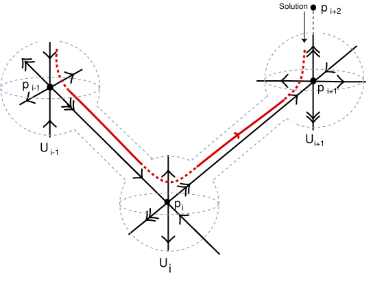
Figure 1. Representation of a heteroclinic channel and a solution following it. Double arrows correspond to the strong expanding directions
Definition 5.

Let ε,δ>0𝜀𝛿0\varepsilon,\delta>0 sufficiently small. We say that system (1) has a heteroclinic channel inside V(ε,δ)𝑉𝜀𝛿V(\varepsilon,\delta) if there exist T0𝑇0T\geq 0 and an open set UU1+𝑈superscriptsubscript𝑈1U\subset U_{1}^{+} of initial conditions such that every solution φ(t,x)𝜑𝑡𝑥\varphi(t,x), xU𝑥𝑈x\in U satisfy (see Figure 1):

  1. (1)

    φ(0,x)=x𝜑0𝑥𝑥\varphi(0,x)=x;

  2. (2)

    t[0,T]for-all𝑡0𝑇\forall t\in[0,T], φ(t,x)V(ε,δ)𝜑𝑡𝑥𝑉𝜀𝛿\varphi(t,x)\in V(\varepsilon,\delta);

  3. (3)

    i{1,,N}for-all𝑖1superscript𝑁\forall i\in\{1,\ldots,N^{\star}\}, there exists a finite sequence (ti)isubscriptsubscript𝑡𝑖𝑖(t_{i})_{i}, ti<Tsubscript𝑡𝑖𝑇t_{i}<T, such that φ(ti,x)Ui𝜑subscript𝑡𝑖𝑥subscript𝑈𝑖\varphi(t_{i},x)\in U_{i}.

The next result says that the occurrence of a heteroclinic channel inside V(ε,δ)𝑉𝜀𝛿V(\varepsilon,\delta) is a robust property (provided ε>0𝜀0\varepsilon>0 and δ>0𝛿0\delta>0 are sufficiently small).

Theorem 1 ([1, 27], adapted).

Let ε,δ>0𝜀𝛿0\varepsilon,\delta>0 sufficiently small. If (1) satisfies the Hypotheses (H1)(H4), then:

  1. (1)

    there exists a heteroclinic channel inside V(ε,δ)𝑉𝜀𝛿V(\varepsilon,\delta) and

  2. (2)

    there exists a neighbourhood 𝒱𝒱\mathcal{V} of the vector field f𝑓f\in\mathcal{B}, endowed with the C1superscript𝐶1C^{1} norm, and an open set 𝒰𝒱𝒰𝒱\mathcal{U}\subset\mathcal{V} such that the flow of x˙=h(x)˙𝑥𝑥\dot{x}=h(x) has a heteroclinic channel inside V(ε,δ)𝑉𝜀𝛿V(\varepsilon,\delta), for every h𝒰𝒰h\in\mathcal{U}.

Althought the existence of a heteroclinic channel is a robust property, the channel as in Definition 5, might be a transient phenomenon.

3.3. The main result

In the present paper, we prove a stronger version of Theorem 1. We show that if a heteroclinic network ΓΓ\Gamma is asymptotically stable then all connections corresponding to the most positive expanding eigenvalues of the linearization at the equilibria will generically form a part of an attractor in the sense of [24]. Although the existence of the heteroclinic cycle is not C1superscript𝐶1C^{1}-structurally stable, the attracting channel is robust. Numerical results described in [27] show that the action of small noise does not destroy the channel. The term “generic” corresponds to an open condition that be specified later and has the same flavour as [24, Lemma 2.3(h)].

Theorem 2.

If (1) satisfies the Hypotheses (H1)(H4) then, generically, the cycle ΓpΓsuperscriptΓ𝑝Γ\Gamma^{p}\subset\Gamma corresponding to the most positive expanding eigenvalues of the linearization at the equilibria is predominantly asymptotically stable.

In other words, Theorem 2 says that, generically, the strong unstable connections define a predominantly asymptotically stable Milnor attractor within ΓΓ\Gamma that is not Lyapunov stable. Along the proof, the reader will realize that, given a small neighbourhood of ΓpsuperscriptΓ𝑝\Gamma^{p}, there exists a cuspoidal region with asymptotically zero Lebesgue measure such that trajectories are repelled from it as t+𝑡t\rightarrow+\infty.

3.4. Important remarks

In what follows, we discuss the relevance of the hypotheses and we also refer some differences between our main result and others in the literature.

  1. (1)

    Our result is consistent with the numerics of [1, 27] developed in the context of the Generalized Lotka-Volterra model. See also [4]. Our result is completely compatible to that of [6, Prop. 7.6 and 7.8] in which the authors proved that finding trajectories that follow the strong unstable connection within a stable network is a lot more probable than finding those that follow the other connections.

  2. (2)

    Throughout our proof, we assume the absence of transverse eigenvalues to the principal cycle ΓpsuperscriptΓ𝑝\Gamma^{p} – see Remark 2. Moreover, we do not use the fact that the vector field f𝑓f commutes with the action of a compact Lie group. Typically, the fixed-point subspaces forces the generic assumption of Theorem 2 to fail.

  3. (3)

    Theorem 2 is remarkably different to that of [18, 30] in which the leading eigenvalues at the equilibria are non-real. Due to the transversality of the invariant manifolds combined with complex eigenvalues, the horseshoe dynamics does not trap most solutions in the neighbourhood of the cycle. In this case, nearby trajectories seem to be equally distributed between the different connections.

3.5. Kirk and Silber example

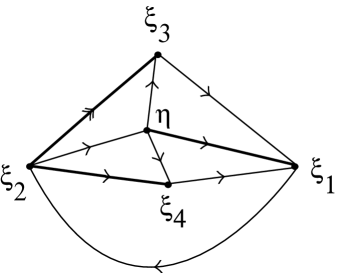
The authors of [17] discussed the case of two competing cycles in a system of ordinary differential equations in 𝐑4superscript𝐑4{\rm\bf R}^{4} with 𝐙24subscriptsuperscript𝐙42{\rm\bf Z}^{4}_{2}–symmetry. Their system has four equilibria ξjsubscript𝜉𝑗\xi_{j} on the coordinate axes at xj=1subscript𝑥𝑗1x_{j}=1, j=1,2,3,4𝑗1234j=1,2,3,4, and two competing cycles (see Figure 2):

ξ1ξ2ξ3ξ1andξ1ξ2ξ4ξ1.formulae-sequencesubscript𝜉1subscript𝜉2subscript𝜉3subscript𝜉1andsubscript𝜉1subscript𝜉2subscript𝜉4subscript𝜉1\xi_{1}\rightarrow\xi_{2}\rightarrow\xi_{3}\rightarrow\xi_{1}\qquad\text{and}\qquad\xi_{1}\rightarrow\xi_{2}\rightarrow\xi_{4}\rightarrow\xi_{1}.

Note that there is an extra saddle equilibrium point whose unstable manifold is two-dimensional, which we call η𝜂\eta. The one-dimensional cycles share the connection [ξ1ξ2]delimited-[]subscript𝜉1subscript𝜉2[\xi_{1}\rightarrow\xi_{2}] and the unstable manifold of ξ2subscript𝜉2\xi_{2} is two-dimensional. Moreover, there are two positive coefficients in the differential equation, e23>0subscript𝑒230e_{23}>0 and e24>0subscript𝑒240e_{24}>0, that correspond to the expanding eigenvalues of ξ2subscript𝜉2\xi_{2}. Numerics allow to prove that, when e23>e24subscript𝑒23subscript𝑒24e_{23}>e_{24}, solutions leaving ξ2subscript𝜉2\xi_{2} in the direction of ξ4subscript𝜉4\xi_{4} pass through a cuspoidal region abutting the connection [ξ1ξ2]delimited-[]subscript𝜉1subscript𝜉2[\xi_{1}\rightarrow\xi_{2}], where both cycles may be attracting. This example does not fit in our study because the connections from ξ2subscript𝜉2\xi_{2} to ξ3subscript𝜉3\xi_{3} involve a one-dimensional and a two-dimensional connecting sets.
Refer to caption
Figure 2. Representation of the simplest configuration for the network considered in [17] (simplified version). The bold lines represent two-dimensional connections; thin lines correspond to one-dimensional connections. Double arrows correspond to the strong expanding directions (case e23>e24subscript𝑒23subscript𝑒24e_{23}>e_{24}); η𝜂\eta corresponds to the extra saddle equilibrium.

4. Linearization and Return Maps

In order to study homo and heteroclinic bifurcations, two approaches have been taken. In the first one, due to Shilnikov and rigorously proved in Deng [8], one rewrites the differential equation in its integral form and uses smoothness results for the integral equations to derive approximations of the Poincaré map. A different technique, used in [31] and coworkers, uses linearization results obtained via a normal form procedure. In this paper, we are going to use the second approach; we establish local coordinates near the hyperbolic equilibria and define some terminology that will be used in the rest of the paper.

Let i{1,,N}𝑖1𝑁i\in\{1,\ldots,N\}. Since pisubscript𝑝𝑖p_{i} is a hyperbolic equilibrium of (1), by the invariant manifold theory [12], there exists a C2superscript𝐶2C^{2} local coordinates (x,y)𝐑n𝑥𝑦superscript𝐑𝑛(x,y)\in{\rm\bf R}^{n} in the neighbourhood of pisubscript𝑝𝑖p_{i} so that the local stable manifold of pisubscript𝑝𝑖p_{i} is x=0𝑥0x=0 and the local unstable manifold is y=0𝑦0y=0. This means that we can essentially reduce the problem by looking at some small neighbourhood of pisubscript𝑝𝑖p_{i}. In this case, the linearization of the vector field f𝑓f at pisubscript𝑝𝑖p_{i} may be represented by a diagonal matrix after a C1superscript𝐶1C^{1} change of coordinates. Assume that we may decompose the tangent space into:

(4) Tpi𝐑n=TciTei,subscript𝑇subscript𝑝𝑖superscript𝐑𝑛direct-sum𝑇subscript𝑐𝑖𝑇subscript𝑒𝑖T_{p_{i}}{\rm\bf R}^{n}=T{c_{i}}\oplus T{e_{i}},

where Tci𝑇subscript𝑐𝑖T{c_{i}} and Tei𝑇subscript𝑒𝑖T{e_{i}} are the contracting and the expanding eigenspace at pisubscript𝑝𝑖p_{i}, respectively (details in [22]).

Remark 2.

With the direct sum (4), we are using explicitly that there are no transverse nor radial eigenvalues. Nevertheless our main result is still valid if all eigenvalues in these directions are less than zero.

By (H2), the expanding and contracting tangent spaces Tei𝑇subscript𝑒𝑖Te_{i} and Tci𝑇subscript𝑐𝑖Tc_{i} are assumed to be uisubscript𝑢𝑖u_{i} and sisubscript𝑠𝑖s_{i}–dimensional. Sometimes it will be useful to write x𝐑ui𝑥superscript𝐑subscript𝑢𝑖x\in{\rm\bf R}^{u_{i}} and y𝐑si𝑦superscript𝐑subscript𝑠𝑖y\in{\rm\bf R}^{s_{i}} as (x1,,xui)𝐑sisubscript𝑥1subscript𝑥subscript𝑢𝑖superscript𝐑subscript𝑠𝑖(x_{1},\ldots,x_{u_{i}})\in{\rm\bf R}^{s_{i}} and (y1,,ysi)𝐑sisubscript𝑦1subscript𝑦subscript𝑠𝑖superscript𝐑subscript𝑠𝑖(y_{1},\ldots,y_{s_{i}})\in{\rm\bf R}^{s_{i}}. In a neighbourhood of pisubscript𝑝𝑖p_{i}, hereafter called Uisubscript𝑈𝑖U_{i}, we transform the vector field into the linearized form:

(5) {x˙(i)=A(i)x(i)y˙(i)=B(i)y(i)casessuperscript˙𝑥𝑖superscript𝐴𝑖superscript𝑥𝑖missing-subexpressionsuperscript˙𝑦𝑖superscript𝐵𝑖superscript𝑦𝑖\left\{\begin{array}[]{l}\dot{x}^{(i)}=A^{(i)}x^{(i)}\\ \\ \dot{y}^{(i)}=B^{(i)}y^{(i)}\\ \end{array}\right.

where A𝐴A and B𝐵B have all positive and negative eigenvalues, respectively. The conditions for C1superscript𝐶1C^{1}–linearization of Hartman [11] of (H2) show that linearization is not possible for subsets of points on the lines defined by resonances (i.e. is a generic condition). The restrictions are a set of zero Lebesgue measure in the parameter space and place no serious constraint on the analysis that follows.
Refer to caption
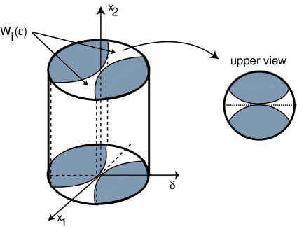
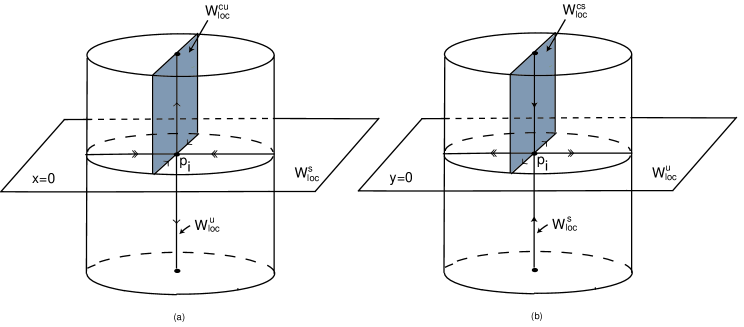
Figure 3. Neighbourhood of pisubscript𝑝𝑖p_{i}. Representation of the cross sections (a): ΣiinsubscriptsuperscriptΣ𝑖𝑛𝑖\Sigma^{in}_{i} and (b): ΣioutsubscriptsuperscriptΣ𝑜𝑢𝑡𝑖\Sigma^{out}_{i}. Trajectories starting at interior points of ΣiinsubscriptsuperscriptΣ𝑖𝑛𝑖\Sigma^{in}_{i} go inside Uisubscript𝑈𝑖U_{i} in positive time. Trajectories starting at interior points of ΣioutsubscriptsuperscriptΣ𝑜𝑢𝑡𝑖\Sigma^{out}_{i} go outside Uisubscript𝑈𝑖U_{i} in positive time.

4.1. Local coordinates and cross sections

Let i{1,,N}𝑖1𝑁i\in\{1,\ldots,N\}. By scaling the local coordinates of the neighbourhood Uisubscript𝑈𝑖U_{i} of the equilibrium pisubscript𝑝𝑖p_{i}, put A(i)superscript𝐴𝑖A^{(i)} and B(i)superscript𝐵𝑖B^{(i)} into Jordan normal form and write:

A(i)=(λ1(i)000λ2(i)000000λui(i))andB(i)=(λui+1(i)000λui+2(i)000000λn(i)).formulae-sequencesuperscript𝐴𝑖matrixsuperscriptsubscript𝜆1𝑖000superscriptsubscript𝜆2𝑖000000superscriptsubscript𝜆subscript𝑢𝑖𝑖andsuperscript𝐵𝑖matrixsuperscriptsubscript𝜆subscript𝑢𝑖1𝑖000superscriptsubscript𝜆subscript𝑢𝑖2𝑖000000superscriptsubscript𝜆𝑛𝑖A^{(i)}=\begin{pmatrix}\lambda_{1}^{(i)}&0&...&0\\ 0&\lambda_{2}^{(i)}&...&0\\ 0&0&...&0\\ 0&0&...&\lambda_{u_{i}}^{(i)}\end{pmatrix}\qquad\text{and}\qquad B^{(i)}=\begin{pmatrix}-\lambda_{u_{i}+1}^{(i)}&0&...&0\\ 0&-\lambda_{u_{i}+2}^{(i)}&...&0\\ 0&0&...&0\\ 0&0&...&-\lambda_{n}^{(i)}\end{pmatrix}.

Define the cross section Σiin𝐑nsubscriptsuperscriptΣ𝑖𝑛𝑖superscript𝐑𝑛\Sigma^{in}_{i}\subset{\rm\bf R}^{n} as :

Σiin={(x(i),y(i)):y(i)=1}={(x(i),θ(i)),x(i)𝐑ui,θ(i)𝐒si1}.\Sigma^{in}_{i}=\left\{\left(x^{(i)},y^{(i)}\right):\left\|y^{(i)}\right\|=1\right\}=\left\{\left(x^{(i)},\theta^{(i)}\right),x^{(i)}\in{\rm\bf R}^{u_{i}},\theta^{(i)}\in{\rm\bf S}^{s_{i}-1}\right\}.

This set intersects all trajectories approaching some neighbourhood of pisubscript𝑝𝑖p_{i}. Analogously, we may define another cross section:

Σiout={(x(i),y(i)):x(i)=1}={(ϕ(i),y(i)),ϕ(i)𝐒ui1,y(i)𝐑si}.\Sigma^{out}_{i}=\left\{\left(x^{(i)},y^{(i)}\right):\left\|x^{(i)}\right\|=1\right\}=\left\{\left(\phi^{(i)},y^{(i)}\right),\phi^{(i)}\in{\rm\bf S}^{u_{i}-1},y^{(i)}\in{\rm\bf R}^{s_{i}}\right\}.

These cross sections, depicted in Figure 3, are transverse to the flow. By construction, trajectories starting at interior points of ΣiinsubscriptsuperscriptΣ𝑖𝑛𝑖\Sigma^{in}_{i} go inside Uisubscript𝑈𝑖U_{i} in positive time. Trajectories starting at interior points of ΣioutsubscriptsuperscriptΣ𝑜𝑢𝑡𝑖\Sigma^{out}_{i} go outside Uisubscript𝑈𝑖U_{i} in positive time. The sets 𝐒si1superscript𝐒subscript𝑠𝑖1{\rm\bf S}^{s_{i}-1} and 𝐒ui1superscript𝐒subscript𝑢𝑖1{\rm\bf S}^{u_{i}-1} are obtained by identifying the opposite faces of ΣiinsuperscriptsubscriptΣ𝑖𝑖𝑛\Sigma_{i}^{in} and ΣioutsuperscriptsubscriptΣ𝑖𝑜𝑢𝑡\Sigma_{i}^{out}. Intersections between the local invariant manifolds at pisubscript𝑝𝑖p_{i} and cross sections are parametrized by:

Wlocs(pi)Σiin={x(i)=0𝐑ui}andWlocu(pi)Σiout={y(i)=0𝐑si}formulae-sequencesubscriptsuperscript𝑊𝑠𝑙𝑜𝑐subscript𝑝𝑖subscriptsuperscriptΣ𝑖𝑛𝑖superscript𝑥𝑖subscript0superscript𝐑subscript𝑢𝑖andsubscriptsuperscript𝑊𝑢𝑙𝑜𝑐subscript𝑝𝑖subscriptsuperscriptΣ𝑜𝑢𝑡𝑖superscript𝑦𝑖subscript0superscript𝐑subscript𝑠𝑖W^{s}_{loc}(p_{i})\cap\Sigma^{in}_{i}=\left\{x^{(i)}=0_{{\rm\bf R}^{u_{i}}}\right\}\qquad\text{and}\qquad W^{u}_{loc}(p_{i})\cap\Sigma^{out}_{i}=\left\{y^{(i)}=0_{{\rm\bf R}^{s_{i}}}\right\}

4.2. Time of flight

Let i{1,,N}𝑖1𝑁i\in\{1,\ldots,N\}. Hereafter, when we refer 𝐑uiΣiinsuperscript𝐑subscript𝑢𝑖superscriptsubscriptΣ𝑖𝑖𝑛{\rm\bf R}^{u_{i}}\subset\Sigma_{i}^{in} we mean 𝐑ui×{0𝐒si1}Σiinsuperscript𝐑subscript𝑢𝑖subscript0superscript𝐒subscript𝑠𝑖1superscriptsubscriptΣ𝑖𝑖𝑛{\rm\bf R}^{u_{i}}\times\{0_{{\rm\bf S}^{s_{i}-1}}\}\subset\Sigma_{i}^{in}. The same for ΣioutsuperscriptsubscriptΣ𝑖𝑜𝑢𝑡\Sigma_{i}^{out}. Define implicitly the map

Ti:𝐑ui\{0𝐑ui}Σiin𝐑0+:subscript𝑇𝑖\superscript𝐑subscript𝑢𝑖subscript0superscript𝐑subscript𝑢𝑖superscriptsubscriptΣ𝑖𝑖𝑛subscriptsuperscript𝐑0T_{i}:{\rm\bf R}^{u_{i}}\backslash\{0_{{\rm\bf R}^{u_{i}}}\}\subset\Sigma_{i}^{in}\rightarrow{\rm\bf R}^{+}_{0}

as x(i)=1.normsuperscript𝑥𝑖1\left\|x^{(i)}\right\|=1. In other terms, the map Tisubscript𝑇𝑖T_{i} is defined in such a way that:

j=1ui(xj(i))2exp(2λj(i)Ti(x(i)))=1.superscriptsubscript𝑗1subscript𝑢𝑖superscriptsuperscriptsubscript𝑥𝑗𝑖22superscriptsubscript𝜆𝑗𝑖subscript𝑇𝑖superscript𝑥𝑖1\sum_{j=1}^{u_{i}}\left(x_{j}^{(i)}\right)^{2}\exp\left({2\lambda_{j}^{(i)}T_{i}\left(x^{(i)}\right)}\right)=1.

The map Tisubscript𝑇𝑖T_{i} gives the transit time that the solution with initial condition (x(i),y(i))superscript𝑥𝑖superscript𝑦𝑖\left(x^{(i)},y^{(i)}\right) spends inside Uisubscript𝑈𝑖U_{i}. Define also the map τ(i):𝐑ui\{0𝐑ui}𝐒ui1:superscript𝜏𝑖\superscript𝐑subscript𝑢𝑖subscript0superscript𝐑subscript𝑢𝑖superscript𝐒subscript𝑢𝑖1\tau^{(i)}:{\rm\bf R}^{u_{i}}\backslash\{0_{{\rm\bf R}^{u_{i}}}\}\rightarrow{\rm\bf S}^{u_{i}-1} by

τ(i)(x1(i),,xui(i))=(τ1(i)(x(i)),,τui(i)(x(i)))whereτj(i)(x(i))=exp(λjTi(x(i)))xj(i),formulae-sequencesuperscript𝜏𝑖superscriptsubscript𝑥1𝑖superscriptsubscript𝑥subscript𝑢𝑖𝑖superscriptsubscript𝜏1𝑖superscript𝑥𝑖superscriptsubscript𝜏subscript𝑢𝑖𝑖superscript𝑥𝑖wheresuperscriptsubscript𝜏𝑗𝑖superscript𝑥𝑖subscript𝜆𝑗subscript𝑇𝑖superscript𝑥𝑖superscriptsubscript𝑥𝑗𝑖\tau^{(i)}\left(x_{1}^{(i)},\ldots,x_{u_{i}}^{(i)}\right)=\left(\tau_{1}^{(i)}\left(x^{(i)}\right),\ldots,\tau_{u_{i}}^{(i)}\left(x^{(i)}\right)\right)\quad\text{where}\quad\tau_{j}^{(i)}\left(x^{(i)}\right)=\exp\left({\lambda_{j}T_{i}\left(x^{(i)}\right)}\right)x_{j}^{(i)},

for j=1,,ui.𝑗1subscript𝑢𝑖j=1,\ldots,{u_{i}}. For all i{1,,N}𝑖1𝑁i\in\{1,\ldots,N\} and j{1,,n}𝑗1𝑛j\in\{1,\ldots,n\}, we know that τ(i)𝐒ui1superscript𝜏𝑖superscript𝐒subscript𝑢𝑖1\tau^{(i)}\in{\rm\bf S}^{{u_{i}}-1}. Thus |τj(i)|1superscriptsubscript𝜏𝑗𝑖1\left|\tau_{j}^{(i)}\right|\leq 1 for all j𝑗j. In particular, for j=1𝑗1j=1, we get:

|τ1(i)(x(i))|=|exp(λ1Ti(x(i)))x1(i)|=|exp(λ1Ti(x(i)))||x1(i)|1.superscriptsubscript𝜏1𝑖superscript𝑥𝑖subscript𝜆1subscript𝑇𝑖superscript𝑥𝑖superscriptsubscript𝑥1𝑖subscript𝜆1subscript𝑇𝑖superscript𝑥𝑖superscriptsubscript𝑥1𝑖1\left|\tau_{1}^{(i)}\left(x^{(i)}\right)\right|=\left|\exp\left(\lambda_{1}T_{i}\left(x^{(i)}\right)\right)x_{1}^{(i)}\right|=\left|\exp\left(\lambda_{1}T_{i}\left(x^{(i)}\right)\right)\right|\left|x_{1}^{(i)}\right|\leq 1.

It follows straightforwardly that:

(6) |x1(i)|1λ1(i)exp(Ti(x(i))).superscriptsuperscriptsubscript𝑥1𝑖1superscriptsubscript𝜆1𝑖subscript𝑇𝑖superscript𝑥𝑖\left|x_{1}^{(i)}\right|^{-\frac{1}{\lambda_{1}^{(i)}}}\geq\exp\left(T_{i}\left(x^{(i)}\right)\right).

The following three technical results will be useful in the sequel.

Lemma 3.

Let i{1,,N}𝑖1𝑁i\in\{1,\ldots,N\}. The following two inequalities hold:

lnx(i)1λ1(i)<Ti(x(i))<lnx(i)1λui(i).superscriptnormsuperscript𝑥𝑖1superscriptsubscript𝜆1𝑖subscript𝑇𝑖superscript𝑥𝑖superscriptnormsuperscript𝑥𝑖1superscriptsubscript𝜆subscript𝑢𝑖𝑖\ln\left\|x^{(i)}\right\|^{-\frac{1}{\lambda_{1}^{(i)}}}<T_{i}\left(x^{(i)}\right)<\ln\left\|x^{(i)}\right\|^{-\frac{1}{\lambda_{u_{i}}^{(i)}}}.
Proof.

By (H2), since λ1(i)>>λui(i)>0superscriptsubscript𝜆1𝑖superscriptsubscript𝜆subscript𝑢𝑖𝑖0\lambda_{1}^{(i)}>...>\lambda_{{u_{i}}}^{(i)}>0, the following implications hold:

j=1ui(xj(i))2exp(2λj(i)Ti(x(i)))=1superscriptsubscript𝑗1subscript𝑢𝑖superscriptsuperscriptsubscript𝑥𝑗𝑖22superscriptsubscript𝜆𝑗𝑖subscript𝑇𝑖superscript𝑥𝑖1\displaystyle\sum_{j=1}^{u_{i}}\left(x_{j}^{(i)}\right)^{2}\exp\left({2\lambda_{j}^{(i)}T_{i}(x^{(i)})}\right)=1\quad j=1ui(xj(i))2exp(2λ1(i)Ti(x(i)))>1absentsuperscriptsubscript𝑗1subscript𝑢𝑖superscriptsuperscriptsubscript𝑥𝑗𝑖22superscriptsubscript𝜆1𝑖subscript𝑇𝑖superscript𝑥𝑖1\displaystyle\Rightarrow\sum_{j=1}^{u_{i}}\left(x_{j}^{(i)}\right)^{2}\exp\left({2\lambda_{1}^{(i)}T_{i}(x^{(i)})}\right)>1
exp(2λ1(i)Ti(x(i)))j=1ui(xj(i))2>1absent2superscriptsubscript𝜆1𝑖subscript𝑇𝑖superscript𝑥𝑖superscriptsubscript𝑗1subscript𝑢𝑖superscriptsuperscriptsubscript𝑥𝑗𝑖21\displaystyle\Leftrightarrow\exp\left({2\lambda_{1}^{(i)}}T_{i}\left(x^{(i)}\right)\right)\sum_{j=1}^{u_{i}}\left(x_{j}^{(i)}\right)^{2}>1
exp(2λ1(i)Ti(x(i)))>1x(i)2absent2superscriptsubscript𝜆1𝑖subscript𝑇𝑖superscript𝑥𝑖1superscriptnormsuperscript𝑥𝑖2\displaystyle\Leftrightarrow\exp\left({2\lambda_{1}^{(i)}T_{i}\left(x^{(i)}\right)}\right)>\frac{1}{\left\|x^{(i)}\right\|^{2}}
λ1(i)Ti(x(i))>ln(x(i))absentsuperscriptsubscript𝜆1𝑖subscript𝑇𝑖superscript𝑥𝑖normsuperscript𝑥𝑖\displaystyle\Leftrightarrow\lambda_{1}^{(i)}T_{i}\left(x^{(i)}\right)>-\ln\left({\left\|x^{(i)}\right\|}\right)
lnx(i)1λ1(i)<Ti(x(i)).absentsuperscriptnormsuperscript𝑥𝑖1superscriptsubscript𝜆1𝑖subscript𝑇𝑖superscript𝑥𝑖\displaystyle\Leftrightarrow\ln\left\|x^{(i)}\right\|^{-\frac{1}{\lambda_{1}^{(i)}}}<T_{i}\left(x^{(i)}\right).

The first inequality of the lemma is shown; the proof of the other is analogous. ∎

In what follows, recall that if i{1,,N}𝑖1𝑁i\in\{1,\ldots,N\} then βi=(αi)1=λ2(i)λ1(i)<1subscript𝛽𝑖superscriptsubscript𝛼𝑖1superscriptsubscript𝜆2𝑖superscriptsubscript𝜆1𝑖1\beta_{i}=(\alpha_{i})^{-1}=\frac{\lambda_{2}^{(i)}}{\lambda_{1}^{(i)}}<1.

Lemma 4.

Let i{1,,N}𝑖1𝑁i\in\{1,\ldots,N\}. The following inequality holds:

1(τ1(i)(x(i)))2<|x1(i)|2βij=2ui(xj(i))21superscriptsuperscriptsubscript𝜏1𝑖superscript𝑥𝑖2superscriptsuperscriptsubscript𝑥1𝑖2subscript𝛽𝑖superscriptsubscript𝑗2subscript𝑢𝑖superscriptsuperscriptsubscript𝑥𝑗𝑖21-\left(\tau_{1}^{(i)}\left(x^{(i)}\right)\right)^{2}<\left|x_{1}^{(i)}\right|^{-2\beta_{i}}\sum_{j=2}^{u_{i}}\left(x_{j}^{(i)}\right)^{2}
Proof.

The proof runs along the same lines to that of Lemma 3. By (H2), since λ2(i)>>λui(i)>0superscriptsubscript𝜆2𝑖superscriptsubscript𝜆subscript𝑢𝑖𝑖0\lambda_{2}^{(i)}>...>\lambda_{{u_{i}}}^{(i)}>0, the following equalities and inequalities are valid:

1(τ1(i)(x(i)))21superscriptsuperscriptsubscript𝜏1𝑖superscript𝑥𝑖2\displaystyle 1-\left(\tau_{1}^{(i)}\left(x^{(i)}\right)\right)^{2} =j=2ui(τj(i)(x(i)))2absentsuperscriptsubscript𝑗2subscript𝑢𝑖superscriptsuperscriptsubscript𝜏𝑗𝑖superscript𝑥𝑖2\displaystyle=\sum_{j=2}^{u_{i}}\left(\tau_{j}^{(i)}\left(x^{(i)}\right)\right)^{2}
=j=2uiexp(2λj(i)Ti(x(i)))(xj(i))2absentsuperscriptsubscript𝑗2subscript𝑢𝑖2superscriptsubscript𝜆𝑗𝑖subscript𝑇𝑖superscript𝑥𝑖superscriptsuperscriptsubscript𝑥𝑗𝑖2\displaystyle=\sum_{j=2}^{u_{i}}\exp\left(2\lambda_{j}^{(i)}T_{i}\left(x^{(i)}\right)\right)\left(x_{j}^{(i)}\right)^{2}
=j=2uiexp(Ti(x(i)))2λj(i)(xj(i))2\displaystyle=\sum_{j=2}^{u_{i}}\exp\left(T_{i}\left(x^{(i)}\right)\right)^{2\lambda_{j}^{(i)}}\left(x_{j}^{(i)}\right)^{2}
<j=2uiexp(Ti(x(i)))2λ2(i)(xj(i))2\displaystyle<\sum_{j=2}^{u_{i}}\exp\left(T_{i}\left(x^{(i)}\right)\right)^{2\lambda_{2}^{(i)}}\left(x_{j}^{(i)}\right)^{2}
=exp(Ti(x(i)))2λ2(i)j=2ui(xj(i))2\displaystyle=\exp\left(T_{i}\left(x^{(i)}\right)\right)^{2\lambda_{2}^{(i)}}\sum_{j=2}^{u_{i}}\left(x_{j}^{(i)}\right)^{2}
|x1(i)|2βij=2nsi(xj(i))2.absentsuperscriptsuperscriptsubscript𝑥1𝑖2subscript𝛽𝑖superscriptsubscript𝑗2𝑛subscript𝑠𝑖superscriptsuperscriptsubscript𝑥𝑗𝑖2\displaystyle\leq\left|x_{1}^{(i)}\right|^{-2\beta_{i}}\sum_{j=2}^{n-s_{i}}\left(x_{j}^{(i)}\right)^{2}.

The last inequality follows from inequality (6). ∎

Lemma 5.

Let i{1,,N}𝑖1𝑁i\in\{1,\ldots,N\}. Let k𝐑+\{0}𝑘\superscript𝐑0k\in{\rm\bf R}^{+}\backslash\{0\} be such that (x1(i))2>kj=2ui(xj(i))2.superscriptsuperscriptsubscript𝑥1𝑖2𝑘superscriptsubscript𝑗2subscript𝑢𝑖superscriptsuperscriptsubscript𝑥𝑗𝑖2\left(x_{1}^{(i)}\right)^{2}>k\sum_{j=2}^{u_{i}}\left(x_{j}^{(i)}\right)^{2}. Then:

1(τ1(x(i)))2<kβix(i)22βi.1superscriptsubscript𝜏1superscript𝑥𝑖2superscript𝑘subscript𝛽𝑖superscriptnormsuperscript𝑥𝑖22subscript𝛽𝑖1-\left(\tau_{1}\left(x^{(i)}\right)\right)^{2}<k^{-\beta_{i}}\left\|x^{(i)}\right\|^{2-2\beta_{i}}.
Proof.

Let us fix a k𝐑+\{0}𝑘\superscript𝐑0k\in{\rm\bf R}^{+}\backslash\{0\} such that (x1(i))2>kj=2ui(xj(i))2superscriptsuperscriptsubscript𝑥1𝑖2𝑘superscriptsubscript𝑗2subscript𝑢𝑖superscriptsuperscriptsubscript𝑥𝑗𝑖2\left(x_{1}^{(i)}\right)^{2}>k\sum_{j=2}^{u_{i}}\left(x_{j}^{(i)}\right)^{2}. Thus, the following equalities and inequalities hold:

1(τ1(i)(x(i)))21superscriptsuperscriptsubscript𝜏1𝑖superscript𝑥𝑖2\displaystyle 1-\left(\tau_{1}^{(i)}\left(x^{(i)}\right)\right)^{2} =j=2ui(τj(i)(x(i)))2absentsuperscriptsubscript𝑗2subscript𝑢𝑖superscriptsuperscriptsubscript𝜏𝑗𝑖superscript𝑥𝑖2\displaystyle=\sum_{j=2}^{u_{i}}\left(\tau_{j}^{(i)}\left(x^{(i)}\right)\right)^{2}
=j=2uiexp(2λj(i)Ti(x(i)))(xj(i))2absentsuperscriptsubscript𝑗2subscript𝑢𝑖2superscriptsubscript𝜆𝑗𝑖subscript𝑇𝑖superscript𝑥𝑖superscriptsuperscriptsubscript𝑥𝑗𝑖2\displaystyle=\sum_{j=2}^{u_{i}}\exp\left(2\lambda_{j}^{(i)}T_{i}\left(x^{(i)}\right)\right)\left(x_{j}^{(i)}\right)^{2}
<j=2uiexp(Ti(x(i)))2λ2(i)(xj(i))2\displaystyle<\sum_{j=2}^{u_{i}}\exp\left(T_{i}\left(x^{(i)}\right)\right)^{2\lambda_{2}^{(i)}}\left(x_{j}^{(i)}\right)^{2}
=exp(Ti(x(i)))2λ2(i)j=2ui(xj(i))2\displaystyle=\exp\left(T_{i}\left(x^{(i)}\right)\right)^{2\lambda_{2}^{(i)}}\sum_{j=2}^{u_{i}}\left(x_{j}^{(i)}\right)^{2}
|x1(i)|2βij=2ui(xj(i))2(By Remark 6)absentsuperscriptsuperscriptsubscript𝑥1𝑖2subscript𝛽𝑖superscriptsubscript𝑗2subscript𝑢𝑖superscriptsuperscriptsubscript𝑥𝑗𝑖2By Remark 6\displaystyle\leq\left|x_{1}^{(i)}\right|^{-2\beta_{i}}\sum_{j=2}^{u_{i}}\left(x_{j}^{(i)}\right)^{2}\qquad(\text{By Remark }\ref{important to lemma 4})
<kβix(i)22βiabsentsuperscript𝑘subscript𝛽𝑖superscriptnormsuperscript𝑥𝑖22subscript𝛽𝑖\displaystyle<k^{-\beta_{i}}\left\|x^{(i)}\right\|^{2-2{\beta_{i}}}

The hypothesis is used on the last inequality. ∎
Refer to caption
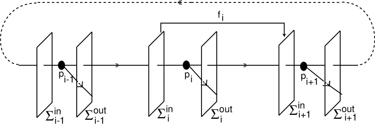
Figure 4. Representation of the maps fi:ΣiinΣi+1in:subscript𝑓𝑖superscriptsubscriptΣ𝑖𝑖𝑛superscriptsubscriptΣ𝑖1𝑖𝑛f_{i}:\Sigma_{i}^{in}\rightarrow\Sigma_{i+1}^{in} and F:Σ1inΣ1in:𝐹superscriptsubscriptΣ1𝑖𝑛superscriptsubscriptΣ1𝑖𝑛F:\Sigma_{1}^{in}\rightarrow\Sigma_{1}^{in}.

4.3. The return map

As in [3], we are interested in a transition model, that we denote by fisubscript𝑓𝑖f_{i}, that carry points from ΣiinsuperscriptsubscriptΣ𝑖𝑖𝑛\Sigma_{i}^{in} to Σi+1insuperscriptsubscriptΣ𝑖1𝑖𝑛\Sigma_{i+1}^{in}. As depicted in Figure 4, the map fi:ΣiinΣi+1in:subscript𝑓𝑖superscriptsubscriptΣ𝑖𝑖𝑛superscriptsubscriptΣ𝑖1𝑖𝑛f_{i}:\Sigma_{i}^{in}\rightarrow\Sigma_{i+1}^{in} may be written as:

fi(x(i),y(i))=(x(i+1),y(i+1))subscript𝑓𝑖superscript𝑥𝑖superscript𝑦𝑖superscript𝑥𝑖1superscript𝑦𝑖1f_{i}\left(x^{(i)},y^{(i)}\right)=\left(x^{(i+1)},y^{(i+1)}\right)

where:

(7) {x(i+1)=M(i)(τ(i)(x(i)))[exp(λui+1(i)Ti(x(i)))y1(i),,exp(λn(i)Ti(x(i)))ysi(i)]𝐑ui+1y(i+1)=γ(i)(τ(i)(x(i)))𝐒si+11casessuperscript𝑥𝑖1superscript𝑀𝑖superscript𝜏𝑖superscript𝑥𝑖superscriptsubscript𝜆subscript𝑢𝑖1𝑖subscript𝑇𝑖superscript𝑥𝑖superscriptsubscript𝑦1𝑖superscriptsubscript𝜆𝑛𝑖subscript𝑇𝑖superscript𝑥𝑖superscriptsubscript𝑦subscript𝑠𝑖𝑖superscript𝐑subscript𝑢𝑖1superscript𝑦𝑖1superscript𝛾𝑖superscript𝜏𝑖superscript𝑥𝑖superscript𝐒subscript𝑠𝑖11\left\{\begin{array}[]{l}x^{(i+1)}=M^{(i)}\left(\tau^{(i)}\left(x^{(i)}\right)\right)\left[\exp\left({-\lambda_{u_{i}+1}^{(i)}T_{i}\left(x^{(i)}\right)}\right)y_{1}^{(i)},...,\exp\left({-\lambda_{n}^{(i)}T_{i}\left(x^{(i)}\right)}\right)y_{s_{i}}^{(i)}\right]\in{\rm\bf R}^{u_{i+1}}\par\\ y^{(i+1)}=\gamma^{(i)}\left(\tau^{(i)}\left(x^{(i)}\right)\right)\in{\rm\bf S}^{s_{i+1}-1}\end{array}\right.

where N+11superscript𝑁11N^{\star}+1\equiv 1 and M(i):𝐒ui1GL(𝐑ui+1):superscript𝑀𝑖superscript𝐒subscript𝑢𝑖1𝐺𝐿superscript𝐑subscript𝑢𝑖1M^{(i)}:{\rm\bf S}^{u_{i}-1}\rightarrow GL({\rm\bf R}^{u_{i+1}}) and γ(i):𝐒ui1𝐒si+11:superscript𝛾𝑖superscript𝐒subscript𝑢𝑖1superscript𝐒subscript𝑠𝑖11\gamma^{(i)}:{\rm\bf S}^{u_{i}-1}\rightarrow{\rm\bf S}^{s_{i+1}-1} are smooth maps. Here, by smooth, we mean at least C1superscript𝐶1C^{1}.

Now let F:Σ1inΣ1in:𝐹superscriptsubscriptΣ1𝑖𝑛superscriptsubscriptΣ1𝑖𝑛F:\Sigma_{1}^{in}\rightarrow\Sigma_{1}^{in} be F=fNfN1f1𝐹subscript𝑓superscript𝑁subscript𝑓superscript𝑁1subscript𝑓1F=f_{N^{\star}}\circ f_{N^{\star}-1}\circ\ldots\circ f_{1} defined as:

F(x(1),y(1))=(x(1),y(1))𝐹superscript𝑥1superscript𝑦1subscriptsuperscript𝑥1subscriptsuperscript𝑦1F\left(x^{(1)},y^{(1)}\right)=\left(x^{(1)}_{\star},y^{(1)}_{\star}\right)

with:

(8) {x(1)=M(τ(1)(x(1)))[exp(λui+1(N)TN(x(N)))y1(N),,exp(λn(N)TN(x(N)))ysi(N)]y(1)=γ(τ(1)(x(1)))casessubscriptsuperscript𝑥1𝑀superscript𝜏1superscript𝑥1superscriptsubscript𝜆subscript𝑢𝑖1superscript𝑁subscript𝑇superscript𝑁superscript𝑥superscript𝑁superscriptsubscript𝑦1superscript𝑁superscriptsubscript𝜆𝑛superscript𝑁subscript𝑇superscript𝑁superscript𝑥superscript𝑁superscriptsubscript𝑦subscript𝑠𝑖superscript𝑁subscriptsuperscript𝑦1𝛾superscript𝜏1superscript𝑥1\left\{\begin{array}[]{l}x^{(1)}_{\star}=M\left(\tau^{(1)}\left(x^{(1)}\right)\right)\left[\exp\left({-\lambda_{u_{i}+1}^{(N^{\star})}T_{N^{\star}}\left(x^{(N^{\star})}\right)}\right)y_{1}^{(N^{\star})},...,\exp\left({-\lambda_{n}^{(N^{\star})}T_{N^{\star}}\left(x^{(N^{\star})}\right)}\right)y_{s_{i}}^{(N^{\star})}\right]\par\\ y^{(1)}_{\star}=\gamma\left(\tau^{(1)}\left(x^{(1)}\right)\right)\end{array}\right.

where:

Mi=1NM(i)andγ=γ(N)γ(1).formulae-sequencenorm𝑀superscriptsubscriptproduct𝑖1superscript𝑁normsuperscript𝑀𝑖and𝛾superscript𝛾superscript𝑁superscript𝛾1\left\|M\right\|\leq\prod_{i=1}^{N^{\star}}\left\|M^{(i)}\right\|\qquad\text{and}\qquad\gamma=\gamma^{(N^{\star})}\circ\ldots\circ\gamma^{(1)}.

5. Proof of the Main Result

The main goal of this section is the proof of Theorem 2. First of all note that, under conditions (H1)–(H4), every trajectory starting in any small neighbourhood of p1subscript𝑝1p_{1} remains in a neighbourhood of ΓΓ\Gamma until it comes to a neighbourhood of pNsubscript𝑝𝑁p_{N} – details in [2]. In the equivariant context, the stability of ΓΓ\Gamma can be obtained using [27] and [22, 23].

The rest of the proof will be based in [1, 3, 5, 8, 17, 24]. We use the previous section to show that for asymptotically stable networks, under Nsuperscript𝑁N^{\star} open conditions on the space of parameters, the majority of trajectories follow a cycle formed by heteroclinic trajectories along the strongly unstable directions.

The proof will be divided into several lemmas. If X𝐑n𝑋superscript𝐑𝑛X\subset{\rm\bf R}^{n}, let Xcsuperscript𝑋𝑐{X}^{c} be the set 𝐑n\X\superscript𝐑𝑛𝑋{\rm\bf R}^{n}\backslash X.

5.1. A repelling cuspoidal region

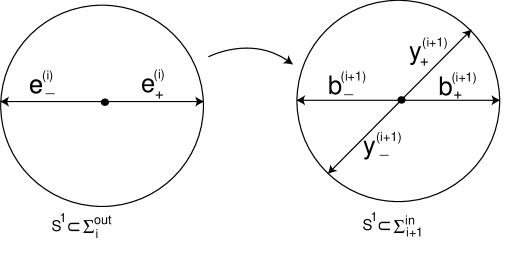
Let i{1,,N}𝑖1𝑁i\in\{1,\ldots,N\}. As suggested by Figure 5 for n=2𝑛2n=2, define:

(9) {e±(i)=(±1,0,,0)𝐒si1Σiouty±(i+1)=γ(i)(e±(i))𝐒si+11Σi+1inb±(i)=(0,0,,±1)𝐒si+11Σiincasessuperscriptsubscript𝑒plus-or-minus𝑖plus-or-minus100superscript𝐒subscript𝑠𝑖1subscriptsuperscriptΣ𝑜𝑢𝑡𝑖superscriptsubscript𝑦plus-or-minus𝑖1superscript𝛾𝑖superscriptsubscript𝑒plus-or-minus𝑖superscript𝐒subscript𝑠𝑖11subscriptsuperscriptΣ𝑖𝑛𝑖1superscriptsubscript𝑏plus-or-minus𝑖00plus-or-minus1superscript𝐒subscript𝑠𝑖11subscriptsuperscriptΣ𝑖𝑛𝑖\left\{\begin{array}[]{l}e_{\pm}^{(i)}=(\pm 1,0,\ldots,0)\in{\rm\bf S}^{s_{i}-1}\subset\Sigma^{out}_{i}\par\\ y_{\pm}^{(i+1)}=\gamma^{(i)}\left(e_{\pm}^{(i)}\right)\in{\rm\bf S}^{s_{i+1}-1}\subset\Sigma^{in}_{i+1}\par\\ b_{\pm}^{(i)}=(0,0,\ldots,\pm 1)\in{\rm\bf S}^{s_{i+1}-1}\subset\Sigma^{in}_{i}\end{array}\right.
Refer to caption
Figure 5. Representation of e±(i)Σioutsuperscriptsubscript𝑒plus-or-minus𝑖subscriptsuperscriptΣ𝑜𝑢𝑡𝑖e_{\pm}^{(i)}\in\Sigma^{out}_{i}, y±(i+1)=γ(i)(e±(i))Σi+1insuperscriptsubscript𝑦plus-or-minus𝑖1superscript𝛾𝑖superscriptsubscript𝑒plus-or-minus𝑖subscriptsuperscriptΣ𝑖𝑛𝑖1y_{\pm}^{(i+1)}=\gamma^{(i)}\left(e_{\pm}^{(i)}\right)\in\Sigma^{in}_{i+1} and b±(i)Σi+1insuperscriptsubscript𝑏plus-or-minus𝑖subscriptsuperscriptΣ𝑖𝑛𝑖1b_{\pm}^{(i)}\in\Sigma^{in}_{i+1}, for n=2𝑛2n=2.

Note that, by construction, the set ΓpsuperscriptΓ𝑝\Gamma^{p} corresponds to the set of connections that cross ΣiinsuperscriptsubscriptΣ𝑖𝑖𝑛\Sigma_{i}^{in} at y(i)=y±(i)superscript𝑦𝑖subscriptsuperscript𝑦𝑖plus-or-minusy^{(i)}=y^{(i)}_{\pm} and then ΣioutsuperscriptsubscriptΣ𝑖𝑜𝑢𝑡\Sigma_{i}^{out} at x(i)=e±(i)superscript𝑥𝑖superscriptsubscript𝑒plus-or-minus𝑖x^{(i)}=e_{\pm}^{(i)}. If δ>0𝛿0\delta>0 is sufficiently small, let us define a δ𝛿\delta-neighbourhood of the heteroclinic connection [pi1pi]delimited-[]subscript𝑝𝑖1subscript𝑝𝑖[p_{i-1}\rightarrow p_{i}] within ΣiinsuperscriptsubscriptΣ𝑖𝑖𝑛\Sigma_{i}^{in} as:

Ei(δ)={(x(i),y(i))Σiin:x(i)<δ}subscript𝐸𝑖𝛿conditional-setsuperscript𝑥𝑖superscript𝑦𝑖superscriptsubscriptΣ𝑖𝑖𝑛normsuperscript𝑥𝑖𝛿E_{i}(\delta)=\left\{\left(x^{(i)},y^{(i)}\right)\in\Sigma_{i}^{in}:\left\|x^{(i)}\right\|<\delta\right\}

and the two following sets:

(10) {i(δ)={(x(i),y(i))Σiin:min{y(i)y+(i),y(i)y(i)}<δ}Bi(δ)=Ei(δ)i(δ)casessubscript𝑖𝛿conditional-setsuperscript𝑥𝑖superscript𝑦𝑖superscriptsubscriptΣ𝑖𝑖𝑛normsuperscript𝑦𝑖superscriptsubscript𝑦𝑖normsuperscript𝑦𝑖superscriptsubscript𝑦𝑖𝛿missing-subexpressionsubscript𝐵𝑖𝛿subscript𝐸𝑖𝛿subscript𝑖𝛿\left\{\begin{array}[]{l}\mathcal{F}_{i}(\delta)=\left\{\left(x^{(i)},y^{(i)}\right)\in\Sigma_{i}^{in}:\min\left\{\left\|y^{(i)}-y_{+}^{(i)}\right\|,\left\|y^{(i)}-y_{-}^{(i)}\right\|\right\}<\delta\right\}\\ \\ B_{i}(\delta)=E_{i}(\delta)\cap\mathcal{F}_{i}(\delta)\end{array}\right.

Let i{1,,N}𝑖1𝑁i\in\{1,\ldots,N\} and ε>0𝜀0\varepsilon>0 sufficiently small.

Definition 6.

A ε𝜀\varepsilon-wedge in ΣiinsuperscriptsubscriptΣ𝑖𝑖𝑛\Sigma_{i}^{in} is defined by:

𝒲i(ε)=subscript𝒲𝑖𝜀absent\displaystyle\mathcal{W}_{i}(\varepsilon)= {(x(i),y(i))Σiin:1(τ1(i)(x(i)))2<ε2}conditional-setsuperscript𝑥𝑖superscript𝑦𝑖superscriptsubscriptΣ𝑖𝑖𝑛1superscriptsuperscriptsubscript𝜏1𝑖superscript𝑥𝑖2superscript𝜀2\displaystyle\left\{\left(x^{(i)},y^{(i)}\right)\in\Sigma_{i}^{in}:1-\left(\tau_{1}^{(i)}\left(x^{(i)}\right)\right)^{2}<\varepsilon^{2}\right\}
=\displaystyle= {(x(i),y(i))Σiin:1exp(2λ1(i)Ti(x(i)))x1(i)<ε2}.conditional-setsuperscript𝑥𝑖superscript𝑦𝑖superscriptsubscriptΣ𝑖𝑖𝑛12superscriptsubscript𝜆1𝑖subscript𝑇𝑖superscript𝑥𝑖superscriptsubscript𝑥1𝑖superscript𝜀2\displaystyle\left\{\left(x^{(i)},y^{(i)}\right)\in\Sigma_{i}^{in}:1-\exp\left(2\lambda_{1}^{(i)}T_{i}\left(x^{(i)}\right)\right)x_{1}^{(i)}<\varepsilon^{2}\right\}.
Lemma 6.

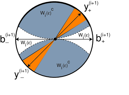
The ε𝜀\varepsilon-wedge 𝒲i(ε)subscript𝒲𝑖𝜀\mathcal{W}_{i}(\varepsilon) contains all initial conditions in ΣiinsuperscriptsubscriptΣ𝑖𝑖𝑛\Sigma_{i}^{in} that are mapped to within ε𝜀\varepsilon of Wlocuu(pi)subscriptsuperscript𝑊𝑢𝑢𝑙𝑜𝑐subscript𝑝𝑖W^{uu}_{loc}(p_{i}) by the projection of the local map (near pisubscript𝑝𝑖p_{i}) induced by the linearization onto 𝐒si1Σioutsuperscript𝐒subscript𝑠𝑖1superscriptsubscriptΣ𝑖𝑜𝑢𝑡{\rm\bf S}^{s_{i}-1}\subset\Sigma_{i}^{out}.

Proof.

The projection of the local map into 𝐒si1Σioutsuperscript𝐒subscript𝑠𝑖1superscriptsubscriptΣ𝑖𝑜𝑢𝑡{\rm\bf S}^{s_{i}-1}\subset\Sigma_{i}^{out} depends on (x1(i),,xsi(i))superscriptsubscript𝑥1𝑖superscriptsubscript𝑥subscript𝑠𝑖𝑖\left(x_{1}^{(i)},\ldots,x_{s_{i}}^{(i)}\right) and is given by τ(i)(x(i))superscript𝜏𝑖superscript𝑥𝑖\tau^{(i)}\left(x^{(i)}\right). The points in ΣiinsuperscriptsubscriptΣ𝑖𝑖𝑛\Sigma_{i}^{in} that are mapped to within ε𝜀\varepsilon of Wlocuu(pi)subscriptsuperscript𝑊𝑢𝑢𝑙𝑜𝑐subscript𝑝𝑖W^{uu}_{loc}(p_{i}) corresponds to that:

|τ1(i)(x(i))1|<εand|τ1(i)(x(i))+1|<ε,formulae-sequencesuperscriptsubscript𝜏1𝑖superscript𝑥𝑖1𝜀andsuperscriptsubscript𝜏1𝑖superscript𝑥𝑖1𝜀\left|\tau_{1}^{(i)}\left(x^{(i)}\right)-1\right|<\varepsilon\qquad\text{and}\qquad\left|\tau_{1}^{(i)}\left(x^{(i)}\right)+1\right|<\varepsilon,

implying that

|τ1(i)(x(i))1||τ1(i)(x(i))+1|=1(τ1(i)(x(i)))2<ε2.superscriptsubscript𝜏1𝑖superscript𝑥𝑖1superscriptsubscript𝜏1𝑖superscript𝑥𝑖11superscriptsuperscriptsubscript𝜏1𝑖superscript𝑥𝑖2superscript𝜀2\left|\tau_{1}^{(i)}\left(x^{(i)}\right)-1\right|\left|\tau_{1}^{(i)}\left(x^{(i)}\right)+1\right|=1-\left(\tau_{1}^{(i)}\left(x^{(i)}\right)\right)^{2}<\varepsilon^{2}.

See Figure 6. ∎

Next result says that 𝒲i(ε)subscript𝒲𝑖𝜀\mathcal{W}_{i}(\varepsilon) has a cuspoidal form, implying that 𝒲i(ε)csubscript𝒲𝑖superscript𝜀𝑐\mathcal{W}_{i}(\varepsilon)^{c} has asymptotically full measure near the set of connections 𝐒si1Σiinsuperscript𝐒subscript𝑠𝑖1subscriptsuperscriptΣ𝑖𝑛𝑖{\rm\bf S}^{s_{i}-1}\subset\Sigma^{in}_{i}. It may be seen as a consequence of Deng’s Strong Lambda Lemma [8].

Proposition 7.

For each i{1,,N}𝑖1𝑁i\in\{1,\ldots,N\}, given ε,δ>0𝜀𝛿0\varepsilon,\delta>0, we have:

(𝒲i(ε)cEi(δ))(Ei(δ))ε2αiδαi1.subscript𝒲𝑖superscript𝜀𝑐subscript𝐸𝑖𝛿subscript𝐸𝑖𝛿superscript𝜀2subscript𝛼𝑖superscript𝛿subscript𝛼𝑖1\frac{\ell(\mathcal{W}_{i}(\varepsilon)^{c}\cap E_{i}(\delta))}{\ell(E_{i}(\delta))}\leq\varepsilon^{-2\alpha_{i}}\delta^{\alpha_{i}-1}.
Refer to caption
Figure 6. Representation of the cusp 𝒲i(ε)Σiinsubscript𝒲𝑖𝜀superscriptsubscriptΣ𝑖𝑖𝑛\mathcal{W}_{i}(\varepsilon)\subset\Sigma_{i}^{in}, where i{1,,N}𝑖1𝑁i\in\{1,\ldots,N\}. The cuspoidal region corresponds to the white region.
Proof.

By Lemma 4, it is easy to see that:

𝒲i(ε)cE(δ)=subscript𝒲𝑖superscript𝜀𝑐𝐸𝛿absent\displaystyle\mathcal{W}_{i}(\varepsilon)^{c}\cap E(\delta)= {(x(i),y(i))Σiin:x(i)<δand1(τ1(i)(x(i)))2ε2}conditional-setsuperscript𝑥𝑖superscript𝑦𝑖superscriptsubscriptΣ𝑖𝑖𝑛formulae-sequencenormsuperscript𝑥𝑖𝛿and1superscriptsuperscriptsubscript𝜏1𝑖superscript𝑥𝑖2superscript𝜀2\displaystyle\left\{\left(x^{(i)},y^{(i)}\right)\in\Sigma_{i}^{in}:\left\|x^{(i)}\right\|<\delta\quad\text{and}\quad 1-\left(\tau_{1}^{(i)}\left(x^{(i)}\right)\right)^{2}\geq\varepsilon^{2}\right\}
\displaystyle\subset {(x(i),y(i))Σiin:x(i)<δandε2(x1(i))2βij=2n(xj(i))2}conditional-setsuperscript𝑥𝑖superscript𝑦𝑖superscriptsubscriptΣ𝑖𝑖𝑛formulae-sequencenormsuperscript𝑥𝑖𝛿andsuperscript𝜀2superscriptsuperscriptsubscript𝑥1𝑖2subscript𝛽𝑖superscriptsubscript𝑗2𝑛superscriptsuperscriptsubscript𝑥𝑗𝑖2\displaystyle\left\{\left(x^{(i)},y^{(i)}\right)\in\Sigma_{i}^{in}:\left\|x^{(i)}\right\|<\delta\quad\text{and}\quad\varepsilon^{2}\left(x_{1}^{(i)}\right)^{2\beta_{i}}\leq\sum_{j=2}^{n}\left(x_{j}^{(i)}\right)^{2}\right\}
\displaystyle\subset {(x(i),y(i))Σiin:x(i)<δand(x1(i))2(δ2ε2)αi}.conditional-setsuperscript𝑥𝑖superscript𝑦𝑖superscriptsubscriptΣ𝑖𝑖𝑛formulae-sequencenormsuperscript𝑥𝑖𝛿andsuperscriptsuperscriptsubscript𝑥1𝑖2superscriptsuperscript𝛿2superscript𝜀2subscript𝛼𝑖\displaystyle\left\{\left(x^{(i)},y^{(i)}\right)\in\Sigma_{i}^{in}:\left\|x^{(i)}\right\|<\delta\quad\text{and}\quad\left(x_{1}^{(i)}\right)^{2}\leq\left(\frac{\delta^{2}}{\varepsilon^{2}}\right)^{\alpha_{i}}\right\}.

The last inclusion follows because:

ε2(x1(i))2βij=2nsi(xj(i))2j=1nsi(xj(i))2=x(i)2<δ2.superscript𝜀2superscriptsuperscriptsubscript𝑥1𝑖2subscript𝛽𝑖superscriptsubscript𝑗2𝑛subscript𝑠𝑖superscriptsuperscriptsubscript𝑥𝑗𝑖2superscriptsubscript𝑗1𝑛subscript𝑠𝑖superscriptsuperscriptsubscript𝑥𝑗𝑖2superscriptnormsuperscript𝑥𝑖2superscript𝛿2\varepsilon^{2}\left(x_{1}^{(i)}\right)^{2\beta_{i}}\leq\sum_{j=2}^{n-s_{i}}\left(x_{j}^{(i)}\right)^{2}\leq\sum_{j=1}^{n-s_{i}}\left(x_{j}^{(i)}\right)^{2}=\left\|x^{(i)}\right\|^{2}<\delta^{2}.

Since βi=(αi)1subscript𝛽𝑖superscriptsubscript𝛼𝑖1\beta_{i}=(\alpha_{i})^{-1}, then:

ε2(x1(i))2βi<δ2(x1(i))2(δ2ε2)αi.formulae-sequencesuperscript𝜀2superscriptsuperscriptsubscript𝑥1𝑖2subscript𝛽𝑖superscript𝛿2superscriptsuperscriptsubscript𝑥1𝑖2superscriptsuperscript𝛿2superscript𝜀2subscript𝛼𝑖\varepsilon^{2}\left(x_{1}^{(i)}\right)^{2\beta_{i}}<\delta^{2}\quad\Rightarrow\quad\left(x_{1}^{(i)}\right)^{2}\leq\left(\frac{\delta^{2}}{\varepsilon^{2}}\right)^{\alpha_{i}}.

Integrating and using Fubini’s Theorem, it follows immediately that:

(𝒲i(ε)cEi(δ))(Ei(δ))ε2αiδαi1.subscript𝒲𝑖superscript𝜀𝑐subscript𝐸𝑖𝛿subscript𝐸𝑖𝛿superscript𝜀2subscript𝛼𝑖superscript𝛿subscript𝛼𝑖1\frac{\ell(\mathcal{W}_{i}(\varepsilon)^{c}\cap E_{i}(\delta))}{\ell(E_{i}(\delta))}\leq{\varepsilon^{-2\alpha_{i}}\delta^{\alpha_{i}-1}}.

By (H4), for all i{1,,N}𝑖1𝑁i\in\{1,\ldots,N\}, we have αi>1subscript𝛼𝑖1\alpha_{i}>1. Hence:

Corollary 8.

For each i{1,,N}𝑖1𝑁i\in\{1,\ldots,N\}, if ε,δ>0𝜀𝛿0\varepsilon,\delta>0 are sufficiently small, the following equality holds:

limδ0(𝒲i(ε)cEi(δ))(Ei(δ))=0.subscript𝛿0subscript𝒲𝑖superscript𝜀𝑐subscript𝐸𝑖𝛿subscript𝐸𝑖𝛿0\lim_{\delta\rightarrow 0}\frac{\ell(\mathcal{W}_{i}(\varepsilon)^{c}\cap E_{i}(\delta))}{\ell(E_{i}(\delta))}=0.

5.2. Uniform convergence

The next result says that the image of the wedge 𝒲i(ε)subscript𝒲𝑖𝜀\mathcal{W}_{i}(\varepsilon) under fisubscript𝑓𝑖f_{i} lies in a neighbourhood of y±(i+1)subscriptsuperscript𝑦𝑖1plus-or-minusy^{(i+1)}_{\pm}.

Lemma 9.

For each i{1,,N}𝑖1𝑁i\in\{1,\ldots,N\}, there is ε1(i)>0superscriptsubscript𝜀1𝑖0\varepsilon_{1}^{(i)}>0 such that for all ε[0,ε1(i)]𝜀0superscriptsubscript𝜀1𝑖\varepsilon\in\left[0,\varepsilon_{1}^{(i)}\right], we have:

fi(𝒲i(ε))i+1(χiε)whereχi=maxϕ(i)𝐒si1dγ(i)dϕ(i).formulae-sequencesubscript𝑓𝑖subscript𝒲𝑖𝜀subscript𝑖1subscript𝜒𝑖𝜀wheresubscript𝜒𝑖subscriptsuperscriptitalic-ϕ𝑖superscript𝐒subscript𝑠𝑖1norm𝑑superscript𝛾𝑖𝑑superscriptitalic-ϕ𝑖f_{i}(\mathcal{W}_{i}(\varepsilon))\subset\mathcal{F}_{i+1}\left(\chi_{i}\varepsilon\right)\qquad\text{where}\qquad\chi_{i}=\max_{\phi^{(i)}\in\,{\rm\bf S}^{s_{i}-1}}\left\|\frac{d\gamma^{(i)}}{d\phi^{(i)}}\right\|.
Proof.

We want to prove that if (x(i+1),y(i+1))fi(𝒲i(ε))superscript𝑥𝑖1superscript𝑦𝑖1subscript𝑓𝑖subscript𝒲𝑖𝜀\left(x^{(i+1)},y^{(i+1)}\right)\in f_{i}(\mathcal{W}_{i}(\varepsilon)), then (x(i+1),y(i+1))i+1(χiε)superscript𝑥𝑖1superscript𝑦𝑖1subscript𝑖1subscript𝜒𝑖𝜀\left(x^{(i+1)},y^{(i+1)}\right)\in\mathcal{F}_{i+1}(\chi_{i}\varepsilon). Indeed, if (x(i+1),y(i+1))fi(𝒲i(ε))superscript𝑥𝑖1superscript𝑦𝑖1subscript𝑓𝑖subscript𝒲𝑖𝜀\left(x^{(i+1)},y^{(i+1)}\right)\in f_{i}(\mathcal{W}_{i}(\varepsilon)), then there exists (x(i),y(i))𝒲i(ε)superscript𝑥𝑖superscript𝑦𝑖subscript𝒲𝑖𝜀\left(x^{(i)},y^{(i)}\right)\in\mathcal{W}_{i}(\varepsilon) such that

fi(x(i),y(i))=(x(i+1),y(i+1)).subscript𝑓𝑖superscript𝑥𝑖superscript𝑦𝑖superscript𝑥𝑖1superscript𝑦𝑖1f_{i}\left(x^{(i)},y^{(i)}\right)=\left(x^{(i+1)},y^{(i+1)}\right).

Since (x(i),y(i))𝒲i(ε)superscript𝑥𝑖superscript𝑦𝑖subscript𝒲𝑖𝜀\left(x^{(i)},y^{(i)}\right)\in\mathcal{W}_{i}(\varepsilon) then, by Lemma 6, we have y(i)e±(i)<εnormsuperscript𝑦𝑖superscriptsubscript𝑒plus-or-minus𝑖𝜀\left\|y^{(i)}-e_{\pm}^{(i)}\right\|<\varepsilon. Therefore,

y(i+1)γ(i)(e±(i))normsuperscript𝑦𝑖1superscript𝛾𝑖superscriptsubscript𝑒plus-or-minus𝑖\displaystyle\left\|y^{(i+1)}-\gamma^{(i)}\left(e_{\pm}^{(i)}\right)\right\| =γ(i)(y(i))γ(i)(e±(i))absentnormsuperscript𝛾𝑖superscript𝑦𝑖superscript𝛾𝑖superscriptsubscript𝑒plus-or-minus𝑖\displaystyle=\left\|\gamma^{(i)}\left(y^{(i)}\right)-\gamma^{(i)}\left(e_{\pm}^{(i)}\right)\right\|
maxϕ(i)𝐒si1dγ(i)dϕ(i)y(i)e±(i)absentsubscriptsuperscriptitalic-ϕ𝑖superscript𝐒subscript𝑠𝑖1norm𝑑superscript𝛾𝑖𝑑superscriptitalic-ϕ𝑖normsuperscript𝑦𝑖superscriptsubscript𝑒plus-or-minus𝑖\displaystyle\leq\max_{\phi^{(i)}\in{\rm\bf S}^{s_{i}-1}}\left\|\frac{d\gamma^{(i)}}{d\phi^{(i)}}\right\|\left\|y^{(i)}-e_{\pm}^{(i)}\right\|
<χiε.absentsubscript𝜒𝑖𝜀\displaystyle<\chi_{i}\varepsilon.

Since μi>1subscript𝜇𝑖1\mu_{i}>1 and ρisubscript𝜌𝑖\rho_{i} is the midpoint of the interval [1,μi]𝐑+1subscript𝜇𝑖superscript𝐑\left[1,\mu_{i}\right]\subset{\rm\bf R}^{+}, it follows that μi>ρi>1subscript𝜇𝑖subscript𝜌𝑖1\mu_{i}>\rho_{i}>1 (by (H4)).

Lemma 10.

For each i{1,,N}𝑖1𝑁i\in\{1,\ldots,N\}, there exists ε2(i)>0superscriptsubscript𝜀2𝑖0\varepsilon_{2}^{(i)}>0 such that for all ε[0,ε2(i)]𝜀0superscriptsubscript𝜀2𝑖\varepsilon\in\left[0,\varepsilon_{2}^{(i)}\right], we have:

fi(Ei(ε))Ei+1(ζiερi)whereζi=maxϕ(i)𝐒si1M(i)(ϕ(i)).formulae-sequencesubscript𝑓𝑖subscript𝐸𝑖𝜀subscript𝐸𝑖1subscript𝜁𝑖superscript𝜀subscript𝜌𝑖wheresubscript𝜁𝑖subscriptsuperscriptitalic-ϕ𝑖superscript𝐒subscript𝑠𝑖1normsuperscript𝑀𝑖superscriptitalic-ϕ𝑖f_{i}(E_{i}(\varepsilon))\subset E_{i+1}(\zeta_{i}\varepsilon^{\rho_{i}})\qquad\text{where}\qquad\zeta_{i}=\max_{\phi^{(i)}\in{\rm\bf S}^{s_{i}-1}}\left\|M^{(i)}\left(\phi^{(i)}\right)\right\|.
Proof.

We want to prove that if (x(i+1),y(i+1))fi(Ei(ε))superscript𝑥𝑖1superscript𝑦𝑖1subscript𝑓𝑖subscript𝐸𝑖𝜀\left(x^{(i+1)},y^{(i+1)}\right)\in f_{i}(E_{i}(\varepsilon)), then (x(i+1),y(i+1))Ei+1(ερi)superscript𝑥𝑖1superscript𝑦𝑖1subscript𝐸𝑖1superscript𝜀subscript𝜌𝑖\left(x^{(i+1)},y^{(i+1)}\right)\in E_{i+1}(\varepsilon^{\rho_{i}}). Indeed, if (x(i+1),y(i+1))fi(Ei(ε))superscript𝑥𝑖1superscript𝑦𝑖1subscript𝑓𝑖subscript𝐸𝑖𝜀\left(x^{(i+1)},y^{(i+1)}\right)\in f_{i}(E_{i}(\varepsilon)) then there exists (x(i),y(i))Ei(ε)superscript𝑥𝑖superscript𝑦𝑖subscript𝐸𝑖𝜀\left(x^{(i)},y^{(i)}\right)\in E_{i}(\varepsilon), i.e. x(i)<εnormsuperscript𝑥𝑖𝜀\left\|x^{(i)}\right\|<\varepsilon such that:

fi(x(i),y(i))=(x(i+1),y(i+1)).subscript𝑓𝑖superscript𝑥𝑖superscript𝑦𝑖superscript𝑥𝑖1superscript𝑦𝑖1f_{i}\left(x^{(i)},y^{(i)}\right)=\left(x^{(i+1)},y^{(i+1)}\right).

Indeed, by the expression (7), we get:

x(i+1)normsuperscript𝑥𝑖1\displaystyle\left\|x^{(i+1)}\right\| maxϕ(i)𝐒si1M(i)(ϕ(i))exp(λui+1Ti(x(i)))y(i)absentsubscriptsuperscriptitalic-ϕ𝑖superscript𝐒subscript𝑠𝑖1normsuperscript𝑀𝑖superscriptitalic-ϕ𝑖subscript𝜆subscript𝑢𝑖1subscript𝑇𝑖superscript𝑥𝑖normsuperscript𝑦𝑖\displaystyle\leq\max_{\phi^{(i)}\in{\rm\bf S}^{s_{i}-1}}\left\|M^{(i)}\left(\phi^{(i)}\right)\right\|\exp\left(-\lambda_{u_{i}+1}T_{i}\left(x^{(i)}\right)\right)\left\|y^{(i)}\right\|
maxϕ(i)𝐒si1M(i)(ϕ(i))exp(Ti(x(i)))λui+1(i)\displaystyle\leq\max_{\phi^{(i)}\in{\rm\bf S}^{s_{i}-1}}\left\|M^{(i)}\left(\phi^{(i)}\right)\right\|\exp\left({T_{i}\left(x^{(i)}\right)}\right)^{-\lambda_{u_{i}+1}^{(i)}}
maxϕ(i)𝐒si1M(i)(ϕ(i))(x1(i))μiabsentsubscriptsuperscriptitalic-ϕ𝑖superscript𝐒subscript𝑠𝑖1normsuperscript𝑀𝑖superscriptitalic-ϕ𝑖superscriptsuperscriptsubscript𝑥1𝑖subscript𝜇𝑖\displaystyle\leq\max_{\phi^{(i)}\in{\rm\bf S}^{s_{i}-1}}\left\|M^{(i)}\left(\phi^{(i)}\right)\right\|\left(x_{1}^{(i)}\right)^{\mu_{i}}
ζix(i)ρi,absentsubscript𝜁𝑖superscriptnormsuperscript𝑥𝑖subscript𝜌𝑖\displaystyle\leq\zeta_{i}\left\|x^{(i)}\right\|^{\rho_{i}},

and the result follows. ∎

Refer to caption
Figure 7. Representation of the non-degeneracy condition (11): the global maps from ΣioutsuperscriptsubscriptΣ𝑖𝑜𝑢𝑡\Sigma_{i}^{out} to Σi+1insuperscriptsubscriptΣ𝑖1𝑖𝑛\Sigma_{i+1}^{in} are non-degenerate and thus cusps are not mappped within other cusps.

We wish to show that the image of most initial conditions passing through ΣioutsuperscriptsubscriptΣ𝑖𝑜𝑢𝑡\Sigma_{i}^{out} via e±(i)superscriptsubscript𝑒plus-or-minus𝑖e_{\pm}^{(i)} hit Σi+1insuperscriptsubscriptΣ𝑖1𝑖𝑛\Sigma_{i+1}^{in} with nonzero component in the x1,±(i+1)superscriptsubscript𝑥1plus-or-minus𝑖1x_{1,\pm}^{(i+1)} direction, where x1,±(i+1)superscriptsubscript𝑥1plus-or-minus𝑖1x_{1,\pm}^{(i+1)} is the first component of

(11) x±(i+1)=M(i)(e±(i))b±(i).superscriptsubscript𝑥plus-or-minus𝑖1superscript𝑀𝑖superscriptsubscript𝑒plus-or-minus𝑖superscriptsubscript𝑏plus-or-minus𝑖x_{\pm}^{(i+1)}=M^{(i)}\left(e_{\pm}^{(i)}\right)b_{\pm}^{(i)}.

Generically, for each i{1,,N}𝑖1𝑁i\in\{1,\ldots,N\}, x1,±(i+1)(modN)0superscriptsubscript𝑥1plus-or-minusannotated𝑖1pmodsuperscript𝑁0x_{1,\pm}^{(i+1)\pmod{N^{\star}}}\neq 0. This means that the global maps from ΣioutsuperscriptsubscriptΣ𝑖𝑜𝑢𝑡\Sigma_{i}^{out} to Σi+1insuperscriptsubscriptΣ𝑖1𝑖𝑛\Sigma_{i+1}^{in} are generic and thus cusps are not mappped within other cusps.

Lemma 11.

For each i{1,,N}𝑖1𝑁i\in\{1,\ldots,N\}, there exists ε3(i)>0superscriptsubscript𝜀3𝑖0\varepsilon_{3}^{(i)}>0 such that for all ε[0,ε3(i)]𝜀0superscriptsubscript𝜀3𝑖\varepsilon\in\left[0,\varepsilon_{3}^{(i)}\right], we have:

fi(𝒲i(ε3)Ei(ε)i(ε3))𝒲i+1(ε2ρi(1βi)).subscript𝑓𝑖subscript𝒲𝑖subscript𝜀3subscript𝐸𝑖𝜀subscript𝑖subscript𝜀3subscript𝒲𝑖1superscript𝜀2subscript𝜌𝑖1subscript𝛽𝑖f_{i}\left(\mathcal{W}_{i}(\varepsilon_{3})\cap E_{i}(\varepsilon)\cap\mathcal{F}_{i}(\varepsilon_{3})\right)\subset\mathcal{W}_{i+1}\left(\varepsilon^{2\rho_{i}(1-\beta_{i})}\right).
Proof.

First we may find ε3>0subscript𝜀30\varepsilon_{3}>0 such that (x(i),y(i))E(ε3)(ε3)superscript𝑥𝑖superscript𝑦𝑖𝐸subscript𝜀3subscript𝜀3\left(x^{(i)},y^{(i)}\right)\in E(\varepsilon_{3})\cap\mathcal{F}(\varepsilon_{3}). This means that there exists (x1(i+1),,xui(i+1))superscriptsubscript𝑥1𝑖1superscriptsubscript𝑥subscript𝑢𝑖𝑖1\left(x_{1}^{(i+1)},\ldots,x_{u_{i}}^{(i+1)}\right) and k𝐑\{0}𝑘\𝐑0k\in{\rm\bf R}\backslash\{0\} such that:

(x1(i+1),,xui(i+1))=(exp(λui+1(i)Ti(x(i)))y1(i),,exp(λn(i)Ti(x(i)))ysi(i))=k.b±(i+1).formulae-sequencesuperscriptsubscript𝑥1𝑖1superscriptsubscript𝑥subscript𝑢𝑖𝑖1superscriptsubscript𝜆subscript𝑢𝑖1𝑖subscript𝑇𝑖superscript𝑥𝑖superscriptsubscript𝑦1𝑖superscriptsubscript𝜆𝑛𝑖subscript𝑇𝑖superscript𝑥𝑖superscriptsubscript𝑦subscript𝑠𝑖𝑖𝑘superscriptsubscript𝑏plus-or-minus𝑖1\left(x_{1}^{(i+1)},\ldots,x_{u_{i}}^{(i+1)}\right)=\left(\exp\left({-\lambda_{u_{i}+1}}^{(i)}T_{i}\left(x^{(i)}\right)\right)y_{1}^{(i)},...,\exp\left({-\lambda_{n}^{(i)}T_{i}\left(x^{(i)}\right)}\right)y_{s_{i}}^{(i)}\right)=k.b_{\pm}^{(i+1)}.

Since M(i)GL(𝐑ui+1)superscript𝑀𝑖𝐺𝐿superscript𝐑subscript𝑢𝑖1M^{(i)}\in GL({\rm\bf R}^{u_{i+1}}) and τi(x(i))subscript𝜏𝑖superscript𝑥𝑖\tau_{i}\left(x^{(i)}\right) is close to e±(i+1)superscriptsubscript𝑒plus-or-minus𝑖1e_{\pm}^{(i+1)}, we may find k1>0subscript𝑘10k_{1}>0 such that the hypothesis of Lemma 5 holds. Thus, for ε[0,ε3(i)]𝜀0superscriptsubscript𝜀3𝑖\varepsilon\in\left[0,\varepsilon_{3}^{(i)}\right], it follows that:

1(τ1(x(i+1)))2<k1βix(i+1)22βi<ε2ρi(1βi)1superscriptsubscript𝜏1superscript𝑥𝑖12superscriptsubscript𝑘1subscript𝛽𝑖superscriptnormsuperscript𝑥𝑖122subscript𝛽𝑖superscript𝜀2subscript𝜌𝑖1subscript𝛽𝑖1-\left(\tau_{1}\left(x^{(i+1)}\right)\right)^{2}<k_{1}^{-\beta_{i}}\left\|x^{(i+1)}\right\|^{2-2\beta_{i}}<\varepsilon^{2\rho_{i}(1-\beta_{i})}

and we get the result. ∎

5.3. The proof of Theorem 2

Let ε(i)=min{ε1(i),ε2(i),ε3(i)}>0superscriptsubscript𝜀𝑖superscriptsubscript𝜀1𝑖superscriptsubscript𝜀2𝑖superscriptsubscript𝜀3𝑖0\varepsilon_{\star}^{(i)}=\min\left\{\varepsilon_{1}^{(i)},\varepsilon_{2}^{(i)},\varepsilon_{3}^{(i)}\right\}>0. For each i{1,,N}𝑖1superscript𝑁i\in\{1,\ldots,N^{\star}\}, using Lemmas 9, 10 and 11, it follows that for all ε[0,ε(i)]𝜀0superscriptsubscript𝜀𝑖\varepsilon\in\left[0,{\varepsilon_{\star}^{(i)}}\right], the inclusion holds, for i(modN)annotated𝑖pmodsuperscript𝑁i\pmod{N^{\star}}:

fi(𝒲i(ε)Ei(ε)i(ε))𝒲i+1(ερi)Ei+1(ζiερi)i+1(χiερi)subscript𝑓𝑖subscript𝒲𝑖𝜀subscript𝐸𝑖𝜀subscript𝑖𝜀subscript𝒲𝑖1superscript𝜀subscript𝜌𝑖subscript𝐸𝑖1subscript𝜁𝑖superscript𝜀subscript𝜌𝑖subscript𝑖1subscript𝜒𝑖superscript𝜀subscript𝜌𝑖f_{i}\left(\mathcal{W}_{i}\left(\varepsilon\right)\cap E_{i}\left(\varepsilon\right)\cap\mathcal{F}_{i}\left(\varepsilon\right)\right)\subset\mathcal{W}_{i+1}\left(\varepsilon^{{\rho_{i}}}\right)\cap E_{i+1}\left(\zeta_{i}\varepsilon^{{\rho_{i}}}\right)\cap\mathcal{F}_{i+1}(\chi_{i}\varepsilon^{\rho_{i}})

For n𝐍𝑛𝐍n\in{\rm\bf N}, define the sequence:

Ωn=𝒲1(ερn1)E1(ερn1)1(ερn1)whereρ=i=1Nρi.formulae-sequencesubscriptΩ𝑛subscript𝒲1superscript𝜀superscript𝜌𝑛1subscript𝐸1superscript𝜀superscript𝜌𝑛1subscript1superscript𝜀superscript𝜌𝑛1where𝜌superscriptsubscriptproduct𝑖1superscript𝑁subscript𝜌𝑖\Omega_{n}=\mathcal{W}_{1}\left(\varepsilon^{\rho^{n-1}}\right)\cap E_{1}\left(\varepsilon^{{\rho^{n-1}}}\right)\cap\mathcal{F}_{1}\left(\varepsilon^{\rho^{n-1}}\right)\qquad\text{where}\quad\rho=\prod_{i=1}^{N^{\star}}\rho_{i}.

By Lemma 8, this set has asymptotically full Lesbegue measure. Therefore F(Ωn)Ωn+1,𝐹subscriptΩ𝑛subscriptΩ𝑛1F(\Omega_{n})\subset\Omega_{n+1}, implying that points in Ω1subscriptΩ1\Omega_{1} converge uniformly to (0,y±(1))Σ1in0superscriptsubscript𝑦plus-or-minus1subscriptsuperscriptΣ𝑖𝑛1\left(0,y_{\pm}^{(1)}\right)\in\Sigma^{in}_{1}, under iteraction of F𝐹F. This finishes the proof of Theorem 2.

Acknowledgments

The author is very grateful to Valentin Afraimovich, who has sketched the proof of Theorem 2 during the Conference School Dynamics, Bifurcations and Strange Attractors which took place in Nizhny Novgorod - Russia. Also special thanks to Alexander Lohse, Michael Field, Pedro Duarte, José Pedro Gaivão and Telmo Peixe for the fruitful discussions.

The author was partially supported by CMUP (UID/MAT/00144/2013), which is funded by FCT with national (MEC) and European structural funds through the programs FEDER, under the partnership agreement PT2020. AR also acknowledges financial support from Program INVESTIGADOR FCT (IF/00107/2015). Part of this work has been written during AR’s stay in Nizhny Novgorod University, supported by the grant RNF 14-41-00044.

References

  • [1] V. Afraimovich, I. Tristan, R. Huerta, M. Rabinovich, Winnerless competition principle and prediction of the transient dynamics in a Lotka-Volterra model, Chaos 18, 4, 043103, 2008
  • [2] V. Afraimovich, V. Zhigulin, M. Rabinovich, On the origin of reproducible sequential activity in neural circuits, Chaos 14, 1123–1129, 2004
  • [3] P. Ashwin, P. Chossat, Attractors for Robust Heteroclinic Cycles with Continua of Connections, J. Nonlinear Sci., Vol. 8, 103–129, 1998
  • [4] C. Bick, M. Rabinovich, On the occurrence of stable heteroclinic channels in Lotka-Volterra models, Dyn. Syst. 25, No. 1, 97–110, 2010
  • [5] W. Brannath, Heteroclinic networks on the tetrahedron, Nonlinearity, 7, 1367–1384, 1994
  • [6] S. Castro, I. Labouriau, O. Podvigina, A heteroclinic network in mode interaction with symmetry, Dynamical Systems: an international journal, Vol. 25, Issue 3, 359–396, 2010
  • [7] S. Castro, A. Lohse, Stability in simple heteroclinic networks in 𝐑4superscript𝐑4{\rm\bf R}^{4}, Dyn. Syst. 29, No. 4, 451–481, 2014
  • [8] B. Deng, The Shilnikov Problem, Exponential Expansion, Strong λ𝜆\lambda-Lemma, C1superscript𝐶1C^{1} Linearisation and Homoclinic Bifurcation, Journal of Differential Equations, 79 189–231, 1989
  • [9] G.L. dos Reis, Structural stability of equivariant vector fields on two-manifolds, Transactions of the American Math. Soc., 283,2, 633–643, 1984
  • [10] J. Guckenheimer, P. Holmes, Structurally stable heteroclinic cycles, Math. Proc. Camb. Phil. Soc., 103, 189–192, 1988
  • [11] P. Hartman, Ordinary differential equations, Wiley, New York, 1964
  • [12] M. Hirsh, C. Pugh, M. Shub, Invariant manifolds, Lecture Notes in Math., Vol. 583, Springer Verlag
  • [13] J. Hofbauer, K. Sigmund, Evolutionary Games and Population Dynamics, Cambridge University Press, 1998
  • [14] A. J. Homburg, Global Aspects of Homoclinic Bifurcations in Vector Fields, Memoirs of the American Mathematical Society, Vol. 121, No. 578, American Mathematical Society, 1996
  • [15] A. J. Homburg, B. Sandstede, Homoclinic and Heteroclinic Bifurcations in Vector Fields, Handbook of Dynamical Systems, 3, North Holland, Amsterdam, 379–524, 2010
  • [16] Z. Hou, S. Balgent, Heteroclinic limit cycles in competitive Kolmogorov systems, Disc. Cont. Dyn. Syst A, 33(9), 4071–4093, 2013
  • [17] V. Kirk, M. Silber, A competition between heteroclinic cycles, Nonlinearity, 7, 1605–1621, 1994.
  • [18] I. S. Labouriau, A. A. P. Rodrigues, Global generic dynamics close to symmetry, Journal of Differential Equations, Journal of Differential Equations, Vol. 253 (8), 2527–2557, 2012
  • [19] A. M. Lyapunov, The general problem of the stability of motion, Translated by A. T. Fuller, Int. J. Control, 55(3), 531–773, 1992
  • [20] A. Lohse, Attraction properties and non-asymptotic stability of simple heteroclinic cycles and networks in 𝐑4superscript𝐑4{\rm\bf R}^{4}, PhD Thesis, University of Hamburg, Germany, 2014
  • [21] M. Krupa, Robust heteroclinic cycles, Journal of Nonlinear Science, 7, 129–176, 1997
  • [22] M. Krupa, I. Melbourne, Asymptotic stability of heteroclinic cycles in systems with symmetry, Ergod. Th. & Dynam. Sys., 15, 121–147, 1995
  • [23] M. Krupa, I. Melbourne, Asymptotic Stability of Heteroclinic Cycles in Systems with Symmetry II, Proc. Roy. Soc. Edinburgh, No. 134A, 219–232, 2004
  • [24] I. Melbourne, An example of a non-asymptotically stable attractor, Nonlinearity, 4, 835–844, 1991
  • [25] I. Melbourne, M. R. E. Proctor, A. M. Rucklidge, A heteroclinic model of geodynamo reversals and excursions, Dynamo and Dynamics, a Mathematical Challenge (eds. P. Chossat, D. Armbruster and I. Oprea, Kluwer: Dordrecht, 363–370, 2001
  • [26] J. Milnor, On the concept of attractor, Commun. Math. Phy. 99, 177–195, 1985
  • [27] M. Muezzinoglu, I. Tristan, R. Huerta, V. Afraimovich, M. Rabinovich Transient versus attractors in complex networks, International Journal of Bifurcation and Chaos 20,6, 1–23, 2010
  • [28] O. Podvigina, P. Ashwin, On local attraction properties and a stability index for heteroclinic connections, Nonlinearity, 24, 887–929, 2011
  • [29] A. A. P. Rodrigues, Persistent Switching near a Heteroclinic Model for the Geodynamo Problem, Chaos, Solitons & Fractals, 47, 73–86, 2013
  • [30] A. A. P. Rodrigues, Repelling dynamics near a Bykov cycle, Journal of Dynamics and Differential Equations, Vol.25, Issue 3, 605–625, 2013
  • [31] C. Tresser, About some theorems by L. P. Shilnikov, Ann. Inst. H. Poincaré, 40, 441–461, 1984