Location Privacy in Mobile Edge Clouds: A Chaff-based Approach

Abstract

In this paper, we consider user location privacy in mobile edge clouds (MECs). MECs are small clouds deployed at the network edge to offer cloud services close to mobile users, and many solutions have been proposed to maximize service locality by migrating services to follow their users. Co-location of a user and his service, however, implies that a cyber eavesdropper observing service migrations between MECs can localize the user up to one MEC coverage area, which can be fairly small (e.g., a femtocell). We consider using chaff services to defend against such an eavesdropper, with focus on strategies to control the chaffs. Assuming the eavesdropper performs maximum likelihood (ML) detection, we consider both heuristic strategies that mimic the user’s mobility and optimized strategies designed to minimize the detection or tracking accuracy. We show that a single chaff controlled by the optimal strategy or its online variation can drive the eavesdropper’s tracking accuracy to zero when the user’s mobility is sufficiently random. We further propose extended strategies that utilize randomization to defend against an advanced eavesdropper aware of the strategy. The efficacy of our solutions is verified through both synthetic and trace-driven simulations.

I Introduction

While improvement in the coverage of wireless communications brings tons of useful applications to the fingertips of mobile users, this trend also imposes a significant threat on user location privacy. Location privacy refers to safeguarding a mobile user’s location from unintended use. While legitimate use of user location can enable various location-based services (LBS), malicious use of this information can cause harmful consequences such as stalking, blackmailing, and fraud [2].

Existing efforts in protecting user location privacy mostly focus on protecting the information released through the direct channel, i.e., location information intentionally revealed by the user. Since the direct channel is controlled by the user, e.g., by configuring whether/when to share his location with an LBS provider, the user can easily obfuscate his location in the spatial/temporal domain to make sure that his location cannot be distinguished from the locations of many other users [2].

The more challenging problem, however, is how to prevent unintentional release of location information through side channels. In wireless networks, an important side channel is the user’s wireless transmission activity, which can be monitored by an eavesdropper with wireless sensing capabilities to track the user, even if the direct channel is perfectly protected. Since its discovery, a few solutions have been proposed to protect this side channel, e.g., by introducing intermittent radio silence and reducing the transmission power, which can effectively increase the uncertainty for the eavesdropper [3, 4].

Figure 1: Providing services to mobile users via MECs.

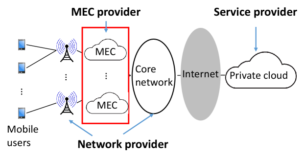
In this work, we investigate the problem in a novel context of mobile edge clouds (MECs) [5], also known as cloudlets [6], mobile micro clouds [7], fog [8], or follow me cloud [9]. As illustrated in Fig. 1, MECs are small clouds that offer a selected set of cloud services from the edge of the mobile network (e.g., base stations). Since its introduction, MEC has attracted tremendous interest from both research communities and industry leaders as a promising approach to improve the performance of cloud services for mobile users [10, 11]. It is also considered the most viable approach to offer cloud services in tactical environments [12]. From the perspective of location privacy, however, this technology opens a new side channel, referred to as the cyber side channel.

Specifically, to deliver the promised performance, MECs need to migrate services (e.g., by migrating virtual machines (VMs) encapsulating the services [13]) to follow the mobile users [9, 14, 5, 7]. For delay-sensitive services (e.g., augmented reality), the service has to remain no more than one hop away from its user to prevent significant degradation in the Quality of Service (QoS) [13]. This implies that a “cyber eavesdropper”, who can observe service migrations among MECs, can track physical movements of the user. Such a cyber eavesdropper can be a hacker that has gained access to the MECs, or an untrusted MEC provider interested in tracking users of certain services. For example, as tactical operations start to use commercial clouds to reduce cost [15], a malicious (or compromised) MEC provider can track tactical users by tracking their services. Cyber eavesdropping is a realistic concern in MECs because of the openness of the MEC ecosystem [10, 16], which increases the risk of introducing both unsecured systems vulnerable to attacks and untrusted providers. Note that we distinguish between the network provider, the MEC provider, and the service provider, where the network provider and the service provider are considered as secure and trusted, but the MEC provider can be insecure and untrusted due to the openness of the MEC ecosystem. The role of the MEC provider is to provide the MEC platform that runs services provided by the service provider, where the MECs and users are interconnected by the network provided by the network provider. Although the spatial resolution of cyber eavesdropping is limited to the coverage of one MEC (e.g., a cell sector), its harm can be severe, as it can be performed without any physical sensing devices, thus potentially at a much lower cost and a much larger scale.

While cyber eavesdropping and wireless eavesdropping are conceptually similar, the defense mechanisms are quite different. Specifically, the existing defense mechanisms for wireless eavesdropping [3, 4] are intrusive in that they modify the user’s transmissions. While it is possible to defend against cyber eavesdropping by stopping the service from following the user, such a mechanism will significantly degrade the QoS for delay-sensitive services [13]. Instead, we consider a non-intrusive mechanism using chaffs. Chaffs are legitimate services launched by the user (or by the network provider on behalf of the user) together with the real service to confuse the eavesdropper about which service the user is actually using. For example, they can be implemented by sending fake service requests and handoff signals to user-specified MECs; see Section II-B for details.

To confuse the eavesdropper, the chaffs must be indistinguishable from the real service. In terms of content, this can be achieved by using independent instances of the same type of service as chaffs. It is, however, insufficient to only make the chaffs indistinguishable in content. For example, a chaff that never migrates can be easily distinguished from a real service that migrates with the mobile user, and a chaff that randomly migrates among MECs can be easily distinguished from a real service that exhibits temporal correlation in its locations. For a chaff to effectively confuse the eavesdropper, its mobility pattern, i.e., where it is launched and whether/where it is migrated, has to resemble the mobility pattern of the real service. Meanwhile, a chaff that always follows the real service (which follows the user) offers no protection for the user’s location privacy. Therefore, the challenge is in controlling the mobility of the chaffs to maximally resemble the real service while minimally co-locating with the real service. To address this challenge, we study the following closely related questions: (i) How will an eavesdropper track a user in the presence of chaffs? (ii) How should the user control the chaffs to defend against the eavesdropper? (iii) What if the user’s defense mechanism is known to the eavesdropper?

I-A Related Work

Most existing work on location privacy refers to protecting the direct channel, where the user intentionally releases his location to access LBS [2]. Most existing solutions, e.g., [2, 17, 18, 19], use location transformations such as spatial/temporal cloaking to satisfy a given anonymity requirement (e.g., $k$-anonymity). The basic idea is to let a trusted server “cloak” a user by replacing the exact user locations by bounding boxes containing sufficiently many other users. While such a strategy can protect the direct channel where the release of location information is explicit, it does not protect side channels such as the cyber side channel considered here.

Besides the direct channel, side channels can also release location information. An important side channel in wireless networks is the transmission activity, which can be monitored by a wireless eavesdropper to track the user. To defend against wireless eavesdropping, mechanisms are proposed to protect senders/receivers using anonymous routing protocols, frequently changing pseudonyms, silent periods, and reduced transmission power [3, 4]. The above mechanisms are intrusive in that they modify the user’s behavior. In contrast, we study another side channel arising in MECs due to correlated user mobility and service mobility, and propose a non-intrusive defense mechanism using chaffs.

The idea of using chaffs to protect user security/privacy has been explored in other contexts. In communication networks, [20] uses dummy packets as chaffs to hide the true traffic rates, and [21] furthers the idea to hide the transmission patterns of multi-hop flows. In cloud computing, [22] proposes to use decoy data to protect the real data during a data theft attack. Similarly, [23] proposes to use decoy applications running on fake inputs to confuse an insider attacker. However, we are the first to study the use of chaff services to protect user location privacy. Besides the novel application context, our problem also requires new methodology. Specifically, as a real service needs to migrate dynamically to follow a mobile user, its mobility pattern (in addition to its content) can be used to identify the service. To effectively protect the user, the chaff services have to resemble the real service in both content and mobility.

Another line of related work is service migrations in MECs. Service migrations in MECs are primarily driven by the need to keep a service close to its user, where the decision on whether to migrate a service depends on both the migration cost (if migrating the service to follow the user) and the communication cost (if serving the user from the original location as the user moves away). Modeling the user’s mobility as a Markov chain (MC), several solutions based on Markov Decision Processes (MDPs) have been proposed to minimize the total cost under 1-D [24, 25] or 2-D mobility models [5, 14]. Here we consider the worst case (in terms of location privacy) that the real service always follows the user, and focus on protecting the user’s location privacy using chaffs. We leave the study of privacy-aware service migration to future work.

I-B Summary of Contributions

We consider the problem of protecting user location privacy using chaffs. Our contributions are:

1) We model the eavesdropper as a maximum likelihood (ML) detector that aims at detecting the user’s trajectory based on multiple observed trajectories.

2) We propose a suite of increasingly sophisticated chaff control strategies for the user: (i) an impersonating (IM) strategy that mimics the user’s mobility, (ii) an ML strategy that maximizes the likelihood of the chaff’s trajectory to mislead the detector, (iii) an optimal offline (OO) strategy that minimizes the eavesdropper’s tracking accuracy based on the user’s entire trajectory, and (iv) an optimal online strategy that minimizes the expected tracking accuracy based on the user’s past trajectory. We show that strategies (i-iii) can be computed in polynomial time. While strategy (iv) is difficult to compute, we propose an alternative myopic online (MO) strategy that is easily computable.

3) Our analysis shows that while the eavesdropper’s tracking accuracy is always non-zero under the IM or ML strategy, it may decay to zero under the OO or MO strategy, where we characterize the condition and the decay rate.

4) We further analyze the robustness of the proposed strategies against an eavesdropper aware of the strategy. We show that while the deterministic strategies (ML, OO, MO) are vulnerable to such an eavesdropper, their robustness can be improved through simple extensions using randomization.

5) We evaluate the proposed strategies on both synthetic and real mobility traces. Our evaluations show that beside the chaff control strategy, the user’s mobility model also has a significant impact on the tracking accuracy. Nevertheless, our strategies (especially OO and MO) can significantly reduce the tracking accuracy even for users with highly predictable mobility, and the same holds for the randomized strategies even if the strategy is known to the eavesdropper.

The rest of the paper is organized as follows. Section II formulates the problem. Section III specifies the model for the eavesdropper. Section IV presents chaff control strategies for the user, whose effectiveness is analyzed in Section V. Section VI analyzes the robustness of the proposed strategies and proposes amendments. Section VII evaluates the performance through simulations. Then Section VIII concludes the paper. All the proofs are provided in the appendix.

II Problem Formulation

II-A Network Model

Given a network field deployed with multiple MECs, we quantize the space into cells such that each cell corresponds to the coverage area of one MEC. Let $\mathcal{L}$ denote the set of cells, which also specifies the set of possible user locations from the perspective of a cyber eavesdropper; let $L:=|\mathcal{L}|$. Suppose that there is a user of interest running a delay-sensitive service (e.g., augmented reality) that must be co-located with the user. We consider delay-sensitive service as it has been identified as one of the most promising applications in future wireless networks [26], while establishing the worst case for location privacy. We leave the study of more flexible services to future work. Note that although our analysis focuses on the single-user scenario, our solution can be independently applied to protect multiple users in a multi-user scenario, where our results provide performance lower bounds as other coexisting users (and their chaffs) offer additional protection.

II-B Eavesdropper and Chaffs

We consider a cyber eavesdropper that observes the trajectories of services as they migrate among the MECs. Such an eavesdropper can be a hacker inside the MEC system, or an untrusted MEC provider (a.k.a. edge operator [16]) that operates the MECs. Under the assumption of delay-sensitive services as in Section II-A, the eavesdropper can track the user by detecting the trajectory of his service.

To prevent detection, the user generates $N-1$ ($N>1$) additional trajectories using chaff services. Each chaff service is an independent instance of the same service that the user is accessing, thus indistinguishable from the real service in content. The chaff services will consume MEC resources, and the cost incurred by these services is the responsibility of the user. In this regard, the parameter $N$ captures the user’s budget for running chaff services. With assistance of the network provider, the user can make a chaff service follow an arbitrary trajectory by sending fake service requests and migration requests to the corresponding MECs, which cause the chaff service to be instantiated or migrated. Alternatively, the service provider can send these requests on behalf of the user. For example, the service provider can offer chaff-based protection of user location privacy as a service option, and if a user wants the protection, he can choose this option and pay an extra cost to the service provider, who will then run chaff services at selected MECs according to a chaff control strategy. Since for a cyber eavesdropper, tracking a user is equivalent to tracking his service, we simply refer to the user’s service as “the user” and the chaff services as “the chaffs”.

II-C Mobility Model

Assume that the user follows a discrete-time ergodic Markovian chain (MC) as in [24, 25, 5], with transition matrix $P=(P(x_{t}|x_{t-1}))_{x_{t},x_{t-1}\in\mathcal{L}}$. Let $\pi:=(\pi(x))_{x\in\mathcal{L}}$ denote his steady-state distribution. Assume that $\pi(x)>0$ for all $x\in\mathcal{L}$. Mobility of the chaffs (i.e., migration of chaff services) is controlled by the user and will be studied later.

For each $u=1,\ldots,N$, let $x_{u,t}\in\mathcal{L}$ denote the location of the $u$-th service in time slot $t$, and $\mathbf{x}_{u}:=(x_{u,t})_{t=1}^{T}$ the trajectory over $T$ slots. Here $u=1$ corresponds to the user, $u=2,\ldots,N$ correspond to the chaffs, and $T\geq 1$ represents the duration of the user’s service.

II-D Location Privacy in the Presence of Chaffs

Our goal is to understand the efficacy of protecting user location privacy using chaffs. We achieve this by studying two closely-related problems:

(i) From the eavesdropper’s perspective: Given $N$ trajectories generated by a user and $N-1$ chaffs, which trajectory belongs to the user?

(ii) From the user’s perspective: Given $N-1$ chaffs, what trajectories should the chaffs follow to cause the worst performance for the eavesdropper?

We measure the eavesdropper’s performance by his tracking accuracy, defined as the time-average probability of correctly tracking the user, i.e., if the eavesdropper believes that the $u$-th trajectory belongs to the user, then his tracking accuracy equals ${1\over T}\sum_{t=1}^{T}\Pr\{x_{u,t}=x_{1,t}\}$. Note that this is different from the detection accuracy, as $u=1$ is sufficient but not necessary for $x_{u,t}=x_{1,t}$.

III Eavesdropper’s Strategy

Given multiple trajectories $\mathbf{x}_{u}:=(x_{u,t})_{t=1}^{T}$ ($u=1,\ldots,N$), the eavesdropper wants to determine which trajectory belongs to the user of interest. We consider a sophisticated eavesdropper who knows the user’s mobility model, i.e., the transition matrix $P$. For example, the eavesdropper can obtain this information by profiling how typical users move in the network field. At this point, we assume that the eavesdropper does not know the user’s chaff control strategy; this assumption will be revised in Section VI.

Intuitively, the eavesdropper should pick the trajectory that best matches the user’s mobility model. Mathematically, this is the trajectory that has the maximum likelihood (ML) among all the trajectories. Under the assumption that all the trajectories have equal prior probability of belonging to the user, the ML trajectory has the maximum posterior probability of belonging to the user. Under the Makovian user mobility model in Section II-C, the ML detector is given by ($[N]:=\{1,\ldots,N\}$)

$$u^{\mbox{\tiny ML}}=\mathop{\arg\max}_{u\in[N]}p(\mathbf{x}_{u})=\mathop{\arg\max}_{u\in[N]}\pi(x_{u,1})\prod_{t=2}^{T}P(x_{u,t}|x_{u,t-1}).$$ (1)

The optimization in (1) can be easily solved in $O(NT)$ time.

Remark: In a multi-user scenario, the detector (1) can also be used to detect a particular user of interest among multiple users, assuming that only the mobility model of the user of interest is known.

IV User’s Strategy

The problem faced by the user is that given $N-1$ chaffs, how to control the mobility of the chaffs, i.e., how to generate the trajectories $\mathbf{x}_{u}$ ($u=2,\ldots,N$), to maximally confuse the eavesdropper. Depending on the precise definition of “confusion”, we have the following chaff control strategies.

IV-A Impersonating Strategy

If the eavesdropper’s strategy is unknown, a safe choice for the user is to make the chaffs appear similar to himself, a strategy referred to as the impersonating (IM) strategy. Under Markovian user mobility, this strategy makes each chaff follow a trajectory generated independently from the same transition matrix $P$ as followed by the user, which naturally mimics the user’s mobility. Under this strategy, all the $N$ trajectories are statistically identical, and therefore any detector, including the ML detector (1), can only make a random guess.

Remark: From the eavesdropper’s perspective, this is the same as a multi-user scenario where all the users follow the same mobility model.

IV-B Maximum Likelihood Strategy

IV-B1 The Strategy

If the user knows that the eavesdropper uses the ML detector (1), then he can design trajectories for the chaffs to intentionally mislead the detector. A chaff’s trajectory can mislead the ML detector only if its likelihood (based on the user’s mobility model) is no smaller than the likelihood of the user’s trajectory. Since the detector is deterministic, it suffices to use a single chaff as at most one chaff (the one with the ML trajectory) will have effect even if multiple chaffs are used.

This idea inspires a strategy referred to as the maximum likelihood (ML) strategy. Letting $\mathcal{L}^{T}$ denote all possible trajectories of length $T$, this strategy controls the chaff to follow a trajectory $\mathbf{x}_{2}$ that achieves the following optimization:

$$\mathbf{x}_{2}=\mathop{\arg\max}_{\mathbf{x}\in\mathcal{L}^{T}}p(\mathbf{x})=\mathop{\arg\max}_{\mathbf{x}\in\mathcal{L}^{T}}\pi(x_{1})\prod_{t=2}^{T}P(x_{t}|x_{t-1}).$$ (2)

IV-B2 The Algorithm

While the space of all possible trajectories ($\mathcal{L}^{T}$) is too large to explore exhaustively, the optimization problem in (2) has a physical interpretation that allows a more efficient solution. We will show that problem (2) can be converted to a shortest-path problem as follows.

The key is to rewrite the optimization (2) as

$$\mathbf{x}_{2}=\mathop{\arg\min}_{\mathbf{x}\in\mathcal{L}^{T}}-\log{\pi(x_{1})}+\sum_{t=2}^{T}(-\log{P(x_{t}|x_{t-1})}).$$ (3)

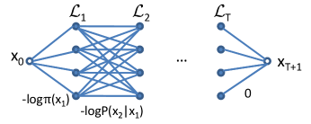
Let $\mathcal{L}_{t}$ ($t=1,\ldots,T$) be a set of vertices representing all possible chaff locations at time $t$ ($|\mathcal{L}_{t}|=|\mathcal{L}|$). As illustrated in Fig. 2, we construct a graph $\mathcal{G}=(V,E)$, with vertices $V=\{x_{0}\}\cup\{x_{T+1}\}\cup\bigcup_{t=1}^{T}\mathcal{L}_{t}$ denoting possible chaff locations at different times ($x_{0}$ and $x_{T+1}$ are virtual locations) and edges $E=(\{x_{0}\}\times\mathcal{L}_{1})\cup(\mathcal{L}_{T}\times\{x_{T+1}\})\cup\bigcup_{t=2}^{T}(\mathcal{L}_{t-1}\times\mathcal{L}_{t})$ denoting possible movements. We assign each edge a cost:

1. edge $(x_{0},x)$ for each $x\in\mathcal{L}_{1}$ has cost $-\log\pi(x)$;

2. edge $(x,x^{\prime})$ for each $x\in\mathcal{L}_{t-1}$ and $x^{\prime}\in\mathcal{L}_{t}$ ($t=2,\ldots,T$) has cost $-\log P(x^{\prime}|x)$;

3. edge $(x,x_{T+1})$ for each $x\in\mathcal{L}_{T}$ has zero cost.

Each possible trajectory $\mathbf{x}=(x_{t})_{t=1}^{T}$ corresponds to a path $(x_{0},x_{1},\ldots,x_{T},x_{T+1})$ from $x_{0}$ to $x_{T+1}$ in $\mathcal{G}$, and the cost of this path, given by the sum of its edge costs, equals the value of the objective function (3) at $\mathbf{x}$. Thus the solution to (3) is essentially the path from $x_{0}$ to $x_{T+1}$ that has the minimum cost, which can be computed by Dijkstra’s algorithm at complexity $O(TL^{2})$. Note that this trajectory only depends on the user’s mobility model and can thus be computed beforehand.

Figure 2: Auxiliary graph for computing the ML trajectory.

Remark: The ML strategy is clearly optimal against the ML detector (1) in minimizing the detection accuracy. This is, however, different from minimizing the tracking accuracy, as the chaff’s trajectory may coincide with the user’s trajectory at times, when the eavesdropper can track the user perfectly.

IV-C Optimal Offline Strategy

IV-C1 The Strategy

The ultimate goal of the user is to prevent himself from being tracked by the eavesdropper. To this end, the chaff’s trajectory not only needs to mislead the detector, but also needs to be as disjoint as possible from the user’s trajectory. For the ML detector (1), the optimal strategy is to let the chaff follow a trajectory that is as disjoint as possible from the user’s trajectory while having a higher likelihood, i.e., the solution $\mathbf{x}_{2}:=(x_{2,t})_{t=1}^{T}$ to the following optimization

$$\min\sum_{t=1}^{T}\mathds{1}_{\{x_{2,t}=x_{1,t}\}}$$ (4)

s.t. $$\,\pi(x_{2,1})\prod_{t=2}^{T}P(x_{2,t}|x_{2,t-1})>\pi(x_{1,1})\prod_{t=2}^{T}P(x_{1,t}|x_{1,t-1}),$$ (5)

where the constraint (5) guarantees that the ML detector will pick the chaff’s trajectory, and the objective (4) minimizes the number of times that the chaff’s trajectory coincides with the user’s trajectory. Again, a single chaff suffices as the detector is deterministic. We refer to this strategy as the optimal offline (OO) strategy, as it is optimal in minimizing the tracking accuracy of an eavesdropper using the ML detector (1) and it requires knowledge of the entire trajectory (including the future trajectory) of the user.

Note that (5) will be infeasible if the user’s trajectory has the maximum likelihood among all the trajectories. In this case, we change the “$>$” in (5) to “$=$” to force the ML detector to make a random guess, but the objective (4) remains valid as we want to minimize the number of times the eavesdropper tracks the user correctly when the detector guesses wrong.

IV-C2 The Algorithm

While a brute-force solution to (4) is infeasible due to the exponentially large solution space, we can solve it by dynamic programming over the weighted graph introduced in Fig. 2. Let $p_{\mathbf{x}_{1}}$ denote the path in this graph corresponding to the user’s trajectory, and $K(p_{\mathbf{x}_{1}})$ the length (sum of edge costs) of this path. Then optimizing (4) subject to (5) is equivalent to finding a path from $x_{0}$ to $x_{T+1}$ with a length less than $K(p_{\mathbf{x}_{1}})$ (or equal to $K(p_{\mathbf{x}_{1}})$ if $p_{\mathbf{x}_{1}}$ is a shortest path) that is as disjoint as possible from $p_{\mathbf{x}_{1}}$. To this end, we introduce $K_{t}(x,i)$ to denote the length of the shortest path from $x\in\mathcal{L}_{t}$ to $x_{T+1}$ that intersects (i.e., sharing vertices) with $p_{\mathbf{x}_{1}}$ at most $i$ times ($0\leq i\leq T-t+1$), and $n_{t}(x,i)$ to denote the next hop neighbor of $x$ on this path.

Initially, $K_{T}(x,1)\equiv 0$ for all $x\in\mathcal{L}_{T}$,

$$K_{T}(x,0) =\left\{\begin{array}[]{ll}0&\mbox{if }x\neq x_{1,T},\\ \infty&\mbox{o.w.,}\end{array}\right.$$ (8)

and $n_{T}(x,i)\equiv x_{T+1}$ for all $x\in\mathcal{L}_{T}$ and $i\in\{0,\>1\}$. For $t=T-1,\ldots,1$,

$$K_{t}(x,i) =\left\{\begin{array}[]{ll}\min\limits_{x^{\prime}\in\mathcal{L}_{t+1}}-\log P(x^{\prime}|x)+K_{t+1}(x^{\prime},i)&\mbox{if }x\neq x_{1,t},\\ \min\limits_{x^{\prime}\in\mathcal{L}_{t+1}}-\log P(x^{\prime}|x)+K_{t+1}(x^{\prime},i-1)&\mbox{o.w.,}\end{array}\right.$$ (11)

$$\hskip 60.00009pt\forall x\in\mathcal{L}_{t},\>i\in\{0,\ldots,T-t+1\},$$ (12)

and $n_{t}(x,i)$ is the value of $x^{\prime}\in\mathcal{L}_{t+1}$ achieving the minimum. By definition, $K_{t}(x,i)\equiv K_{t}(x,T-t+1)$ for all $i>T-t+1$, and $K_{t}(x,i)=\infty$ for $i<0$ (infeasible). At $t=0$, we have

$$K_{0}(x_{0},i) =\min_{x\in\mathcal{L}_{1}}-\log\pi(x)+K_{1}(x,i),~{}\forall i\in\{0,\ldots,T\},$$ (13)

and $n_{0}(x_{0},i)$ is the $x\in\mathcal{L}_{1}$ achieving the minimum.

Then $i^{*}$, defined by the smallest value of $i\in\{0,\ldots,T\}$ satisfying $K_{0}(x_{0},i)<K(p_{\mathbf{x}_{1}})$, is the optimal value of (4) (if infeasible, then $i^{*}$ is the smallest $i$ satisfying $K_{0}(x_{0},i)=K(p_{\mathbf{x}_{1}})$). The optimal chaff’s trajectory $\mathbf{x}_{2}$ is given by:

1. $x_{2,1}=n_{0}(x_{0},i^{*})$, and $i_{1}=i^{*}$;

2. for $t=2,\ldots,T$: $x_{2,t}=n_{t-1}(x_{2,t-1},i_{t-1})$, and $i_{t}=i_{t-1}$ if $x_{2,t-1}\neq x_{1,t-1}$ or $i_{t}=i_{t-1}-1$ otherwise.

See Algorithm 1 for the pseudo code of this strategy. The complexity of this dynamic programming is $O(T^{2}L^{2})$.

input : Space $\mathcal{L}$, user transition matrix $P$, user steady state distribution $\pi$, time horizon $T$, user trajectory $\mathbf{x}_{1}$

output : Chaff trajectory $\mathbf{x}_{2}=(x_{2,t})_{t=1}^{T}$

1 $K(p_{\mathbf{x}_{1}})=-\log{\pi(x_{1,1})}$;

2 foreach $t=2,\ldots,T$ do

3      $K(p_{\mathbf{x}_{1}})=K(p_{\mathbf{x}_{1}})-\log{P(x_{1,t}|x_{1,t-1})}$

4foreach $x\in\mathcal{L}$ do

5      $K_{T}(x,1)=0$;

6       if $x\neq x_{1,T}$ then

7            $K_{T}(x,0)=0$;

8      else

9            $K_{T}(x,0)=\infty$;

10      $n_{T}(x,0)=x_{T+1}$;

11       $n_{T}(x,1)=x_{T+1}$;

12      

13foreach $t=T-1,\ldots,1$ do

14      foreach $x\in\mathcal{L}$ do

15             foreach $i=0,\ldots,T-t+1$ do

16                   if $x\neq x_{1,t}$ then

17                        $j=i$;

18                  else

19                        $j=i-1$;

20                  $K_{t}(x,i)=\min_{x^{\prime}\in\mathcal{L}}-\log{P(x^{\prime}|x)}+K_{t+1}(x^{\prime},j)$;

21                   $n_{t}(x,i)=\mathop{\arg\min}_{x^{\prime}\in\mathcal{L}}-\log{P(x^{\prime}|x)}+K_{t+1}(x^{\prime},j)$;

22                  

23foreach $i=0,\ldots,T$ do

24      $K_{0}(x_{0},i)=\min_{x\in\mathcal{L}}-\log{\pi(x)}+K_{1}(x,i)$;

25       $n_{0}(x_{0},i)=\mathop{\arg\min}_{x\in\mathcal{L}}-\log{\pi(x)}+K_{1}(x,i)$;

26      

27if $K_{0}(x_{0},T)<K(p_{\mathbf{x}_{1}})$ then

28      foreach $i^{*}=0,\ldots,T$ do

29            if $K_{0}(x_{0},i^{*})<K(p_{\mathbf{x}_{1}})$ then

30                  break;

31else

32      foreach $i^{*}=0,\ldots,T$ do

33            if $K_{0}(x_{0},i^{*})=K(p_{\mathbf{x}_{1}})$ then

34                  break;

35$x_{2,1}=n_{0}(x_{0},i^{*})$;

36 $i_{1}=i^{*}$;

37 foreach $t=2,\ldots,T$ do

38      $x_{2,t}=n_{t-1}(x_{2,t-1},i_{t-1})$;

39       if $x_{2,t-1}\neq x_{1,t-1}$ then

40            $i_{t}=i_{t-1}$

41      else

42            $i_{t}=i_{t-1}-1$

Algorithm 1 Optimal Offline (OO) Strategy

IV-D Optimal Online Strategy

IV-D1 The Strategy

In cases where the user’s future trajectory cannot be exactly predicted beforehand, the offline strategy is not applicable. For such cases, we consider the online counterpart of the optimization (4), which only requires knowledge of the user’s past trajectory and the transition probabilities of the user mobility model (defined in Section II-C). As shown below, this problem can be cast as a finite-horizon Markov Decision Process (MDP), which is characterized by a $5$-tuple $(\mathcal{S},\>\mathcal{A},\>\mathcal{T},\>C,\>T)$, defined as:

$\bullet$ The state space $\mathcal{S}=\mathbb{R}\times\mathcal{L}^{2}$ is the space of the triple $(\gamma_{t},x_{1,t},x_{2,t})$, where $\gamma_{t}:=\log p(\mathbf{x}_{1}^{t})-\log p(\mathbf{x}_{2}^{t})$ is the difference between the log-likelihoods of user’s/chaff’s trajectories ($\mathbf{x}_{i}^{t}:=(x_{i,1},\ldots,x_{i,t})$), $x_{1,t}$ is the user location, and $x_{2,t}$ is the chaff location, all at time $t$;

$\bullet$ The action space $\mathcal{A}=\mathcal{L}$ is the set of possible locations that the chaff can move to at any given time;

$\bullet$ The state transition $\mathcal{T}$ includes three transitions (logically) occurring as: (i) $x_{1,t-1}$ transits to a random $x_{1,t}$ with probability $P(x_{1,t}|x_{1,t-1})$; (ii) $x_{2,t-1}$ transits to a (random or deterministic) $x_{2,t}$ according to a control policy $\psi$; (iii) $\gamma_{t-1}$ transits to $\gamma_{t}=\gamma_{t-1}+\log P(x_{1,t}|x_{1,t-1})-\log P(x_{2,t}|x_{2,t-1})$;

$\bullet$ The cost function $C(\gamma_{t},x_{1,t},x_{2,t})=\mathds{1}_{\{x_{2,t}=x_{1,t}\}}+\mathds{1}_{\{x_{2,t}\neq x_{1,t}\}}(\mathds{1}_{\{\gamma_{t}>0\}}+{1\over 2}\mathds{1}_{\{\gamma_{t}=0\}})$;

$\bullet$ The horizon $T$ is the time duration of the user’s trajectory.

Since the cost function $C(\gamma_{t},x_{1,t},x_{2,t})$ represents the per-slot tracking accuracy of the ML detector (1), the control policy $\psi^{\mbox{\tiny OPT}}$ that minimizes the total cost over horizon $T$ is the optimal online chaff control strategy.

Solving this MDP optimally, however, faces both the usual challenge of dimensionality and an unusual challenge that one component of the state ($\gamma_{t}$) has a continuous space. Instead, we consider a commonly used heuristic, the myopic policy, which only minimizes the immediate cost:

$$\psi^{\mbox{\tiny MY}}(\gamma_{t-1},x_{1,t-1},x_{2,t-1},x_{1,t}) :=\mathop{\arg\min}_{x_{2,t}\in\mathcal{L}}C(\gamma_{t},x_{1,t},x_{2,t}),$$ (14)

where $\gamma_{t}$ is completely determined by $\gamma_{t-1}$, $x_{1,t-1}$, $x_{2,t-1}$, $x_{1,t}$, and $x_{2,t}$. However, any efficient MDP solver (e.g., rollout algorithm) is applicable here, and we leave comparison between different solvers to future work.

IV-D2 The Algorithm

Based on (14), we develop a control strategy called the myopic online (MO) strategy. This strategy combines the maximization of the cumulative likelihood and the minimization of the per-slot tracking accuracy: for each $t=1,\ldots,T$, given the user’s location $x_{1,t}$,

1. if the ML location for the chaff $x_{2,t}^{(1)}=\mathop{\arg\max}_{x\in\mathcal{L}}P(x|x_{2,t-1})$ (or $\mathop{\arg\max}_{x\in\mathcal{L}}\pi(x)$ if $t=1$) does not coincide with the user’s location $x_{1,t}$, then move the chaff to $x_{2,t}^{(1)}$;

2. otherwise, if the second ML location for the chaff $x_{2,t}^{(2)}=\mathop{\arg\max}_{x\in\mathcal{L}\setminus\{x_{1,t}\}}P(x|x_{2,t-1})$ (or $\mathop{\arg\max}_{x\in\mathcal{L}\setminus\{x_{1,1}\}}\pi(x)$ if $t=1$) is good enough (i.e., giving an overall likelihood no smaller than that of the user), then move the chaff to $x_{2,t}^{(2)}$;

3. otherwise, move the chaff to $x_{2,t}^{(1)}$.

Note that in the third case, the user will be tracked correctly at $t$ no matter where the chaff moves, and hence we move the chaff to the ML location to maximize the chance of evading tracking in future slots. See Algorithm 2 for the pseudo code of this strategy, where lines 2 and 2 handle case (1), lines 2 and 2 handle case (2), and lines 2 and 2 handle case (3).

input : Space $\mathcal{L}$, user transition matrix $P$, user steady state distribution $\pi$, time horizon $T$

output : Locations of chaff in slots $1,\ldots,T$

1 observe initial user location $x_{1,1}$;

2 compute $x_{2,1}^{(1)}=\mathop{\arg\max}_{x\in\mathcal{L}}\pi(x)$;

3 if $x_{2,1}^{(1)}\neq x_{1,1}$ then

4      $x_{2,1}\leftarrow x_{2,1}^{(1)}$;

5      

6else

7      compute $x_{2,1}^{(2)}=\mathop{\arg\max}_{x\in\mathcal{L}\setminus\{x_{1,1}\}}\pi(x)$;

8       if $\pi(x_{2,1}^{(2)})\geq\pi(x_{1,1})$ then

9            $x_{2,1}\leftarrow x_{2,1}^{(2)}$;

10            

11      else

12            $x_{2,1}\leftarrow x_{2,1}^{(1)}$;

13            

14 $\gamma_{1}\leftarrow\log\pi(x_{1,1})-\log\pi(x_{2,1})$;

15 foreach $t=2,\ldots,T$ do

16       observe new user location $x_{1,t}$;

17       compute $x_{2,t}^{(1)}=\mathop{\arg\max}_{x\in\mathcal{L}}P(x|x_{2,t-1})$;

18       if $x_{2,t}^{(1)}\neq x_{1,t}$ then

19            $x_{2,t}\leftarrow x_{2,t}^{(1)}$;

20            

21      else

22             compute $x_{2,t}^{(2)}=\mathop{\arg\max}_{x\in\mathcal{L}\setminus\{x_{1,t}\}}P(x|x_{2,t-1})$;

23             if $\gamma_{t-1}+\log P(x_{1,t}|x_{1,t-1})-\log P(x_{2,t}^{(2)}|x_{2,t-1})\leq 0$ then

24                  $x_{2,t}\leftarrow x_{2,t}^{(2)}$;

25                  

26            else

27                  $x_{2,t}\leftarrow x_{2,t}^{(1)}$;

28                  

29      $\gamma_{t}\leftarrow\gamma_{t-1}+\log P(x_{1,t}|x_{1,t-1})-\log P(x_{2,t}|x_{2,t-1})$;

30      

Algorithm 2 Myopic Online (MO) Strategy

V Performance Analysis

We now analyze the performance of the proposed strategies in Section IV in terms of the tracking accuracy of the eavesdropper in Section III. We denote the time-average tracking accuracy under each strategy by $P_{\mbox{\tiny IM}}$, $P_{\mbox{\tiny ML}}$, $P_{\mbox{\tiny OO}}$, and $P_{\mbox{\tiny MO}}$.

V-A Tracking Accuracy under IM

Under the IM strategy, the eavesdropper randomly guesses a trajectory for the user. He correctly tracks the user at time $t$ if and only if (i) he guesses the trajectory right, which occurs with probability $1/N$, or (ii) he guesses the trajectory wrong but the guessed trajectory coincides with the user’s trajectory at time $t$. Thus, the overall tracking accuracy equals

$$P_{\mbox{\tiny IM}} ={1\over N}+{N-1\over N}\cdot{1\over T}\sum_{t=1}^{T}\Pr\{x^{\prime}_{t}=x_{t}\},$$ (15)

where $\mathbf{x}^{\prime}=(x^{\prime}_{t})_{t=1}^{T}$ and $\mathbf{x}=(x_{t})_{t=1}^{T}$ are two independent instances of the same MC that describes the user’s mobility. Given the steady-state distribution $\pi$ of this MC, it is easy to see that $\Pr\{x^{\prime}_{t}=x_{t}\}=\sum_{x\in\mathcal{L}}\pi^{2}(x)$. Therefore,

$$P_{\mbox{\tiny IM}} =\Big{(}\sum_{x\in\mathcal{L}}\pi^{2}(x)\Big{)}+{1\over N}\Big{(}1-\sum_{x\in\mathcal{L}}\pi^{2}(x)\Big{)}.$$ (16)

Remark: (i) As the number of chaffs increases, the tracking accuracy under the IM strategy converges monotonically at rate $O(1/N)$. (ii) The limit $\lim_{N\to\infty}P_{\mbox{\tiny IM}}=\sum_{x\in\mathcal{L}}\pi^{2}(x)\geq 1/L$, where the lower bound is achieved if and only if $\pi$ is a uniform distribution. Thus, under the IM strategy, the tracking accuracy is bounded away from zero even with infinite chaffs.

V-B Tracking Accuracy under ML

Under the ML strategy, the chaff’s trajectory $\mathbf{x}_{2}$ is deterministic and is guaranteed to be selected by the ML detector. The tracking accuracy is therefore determined by the fraction of time that the user’s trajectory coincides with $\mathbf{x}_{2}$, i.e.,

$$P_{\mbox{\tiny ML}} ={1\over T}\sum_{t=1}^{T}\Pr\{x_{1,t}=x_{2,t}\}={1\over T}\sum_{t=1}^{T}\pi(x_{2,t}),$$ (17)

where $\mathbf{x}_{2}$ is the solution to (2).

Compared with the value of $\lim_{N\to\infty}P_{\mbox{\tiny IM}}$, $P_{\mbox{\tiny ML}}$ can be either smaller or larger. However, we have a fixed comparison when the following lemma applies.

Lemma V.1.

For any distribution $(\pi(x))_{x\in\mathcal{L}}$, $\sum_{x\in\mathcal{L}}\pi^{2}(x)\leq\max_{x\in\mathcal{L}}\pi(x)$, and “$=$” holds if and only if $(\pi(x))_{x\in\mathcal{L}}$ is a uniform distribution.

Remark: Therefore, if the ML chaff always stays in the same cell (the cell with the maximum steady-state probability), then it is better to use a sufficiently large number of IM chaffs.

V-C Tracking Accuracy under OO

Under the OO strategy, the chaff’s trajectory is designed to yield the minimum tracking accuracy. Therefore, its tracking accuracy is upper-bounded by the tracking accuracy under any suboptimal strategy.

V-C1 Auxiliary Strategy

To bound the tracking accuracy under the OO strategy, we introduce a suboptimal strategy whose tracking accuracy can be analyzed in closed form. This strategy, referred to as the constrained maximum likelihood (CML) strategy, greedily maximizes the likelihood of the chaff’s trajectory under the constraint that the chaff cannot co-locate with the user. That is, given the user’s trajectory $\mathbf{x}_{1}$, the chaff’s trajectory $\mathbf{x}_{2}$ is computed by

1. at $t=1$, $x_{2,1}=\mathop{\arg\max}_{x\in\mathcal{L}\setminus\{x_{1,1}\}}\pi(x)$;

2. at $t>1$, $x_{2,t}=\mathop{\arg\max}_{x\in\mathcal{L}\setminus\{x_{1,t}\}}P(x|x_{2,t-1})$.

Note that CML is actually an online strategy as it never requires the future trajectory of the user.

V-C2 Analysis of Auxiliary Strategy

Under the CML strategy, the chaff’s trajectory is always disjoint from the user’s trajectory, and thus the eavesdropper correctly tracks the user if and only if the ML detector is correct, which occurs only if the user’s trajectory has a likelihood no smaller than that of the chaff’s trajectory. That is, the tracking accuracy under the CML strategy satisfies

$$P_{\mbox{\tiny CML}}\leq\Pr\{p(\mathbf{x}_{1})\geq p(\mathbf{x}_{2})\},$$ (18)

where $\mathbf{x}_{2}$ is generated according to the CML strategy.

As $p(\mathbf{x})=\pi(x_{1})\prod_{t=2}^{T}P(x_{t}|x_{t-1})$, we can define

$$c_{1}(x_{1,1},x_{2,1}):=\log{\pi(x_{1,1})}-\log{\pi(x_{2,1})},$$ (19)

$$c_{t}(x_{1,t},x_{2,t},x_{1,t-1},x_{2,t-1}):=\log{P(x_{1,t}|x_{1,t-1})}$$

$$\hskip 80.00012pt-\log{P(x_{2,t}|x_{2,t-1})},~{}~{}~{}t>1,$$ (20)

and convert $\Pr\{p(\mathbf{x}_{1})\geq p(\mathbf{x}_{2})\}$ to

$$\Pr\{c_{1}(x_{1,1},x_{2,1})+\sum_{t=2}^{T}c_{t}(x_{1,t},x_{2,t},x_{1,t-1},x_{2,t-1})\geq 0\}.$$ (21)

The tracking accuracy under the CML strategy is then upper-bounded by (21).

To bound (21), we consider a new MC formed by $y_{t}:=(x_{1,t},\>x_{2,t})$. This MC is induced by the original MC describing the user’s mobility, with a transition probability

$$P(y_{t}|y_{t-1})=\left\{\begin{array}[]{ll}P(x_{1,t}|x_{1,t-1})&\mbox{if }x_{2,t}=f(x_{1,t},x_{2,t-1}),\\ 0&\mbox{o.w.,}\end{array}\right.$$ (24)

where $f(x_{1,t},x_{2,t-1}):=\mathop{\arg\max}_{x\in\mathcal{L}\setminus\{x_{1,t}\}}P(x|x_{2,t-1})$ is the chaff location at time $t$ under the CML strategy. With a little abuse of notation, let $\pi(y_{t})$ denote the steady-state distribution of the MC $\{y_{t}\}_{t=1}^{\infty}$. For any $\epsilon>0$, let $t_{\mbox{\tiny mix}}(\epsilon)$ denote the $\epsilon$-mixing time of $\{y_{t}\}_{t=1}^{\infty}$ [27]. For the ease of notation, we shorten $c_{t}(x_{1,t},x_{2,t},x_{1,t-1},x_{2,t-1})$ to $c_{t}$.

Our idea is to apply concentration bounds to show that (21) diminishes with $T$ if $\mathbb{E}[c_{t}]<0$. However, since $c_{t}$ is a function of $y_{t}$ and $y_{t-1}$, $c_{t}$’s are correlated, which makes existing concentration bounds inapplicable. To address this challenge, we decompose $\sum_{t}c_{t}$ into $w$ summations $\sum_{k}c_{kw+i}$ ($i=1,\ldots,w$) such that each summation is over a sub-chain consisting of elements that are $w$ steps apart, as illustrated in Fig. 3. Intuitively, if $w$ is sufficiently large, correlation within a sub-chain will be sufficiently weak such that the usual concentration bounds hold for summation over the sub-chain.

Figure 3: Decomposing a chain into $w$ sub-chains.

To formalize this intuition, we prove the following lemma. Define (noting that $c_{t}$ is determined by $y_{t}$ and $y_{t-1}$)

$$g(y_{t-1}) :=\mathbb{E}[c_{t}|y_{t-1}]=\sum_{y_{t}\in\mathcal{L}^{2}}P(y_{t}|y_{t-1})c_{t}.$$ (25)

Lemma V.2.

For any $\epsilon>0$, if $w=t_{\mbox{\tiny mix}}(\epsilon)+1$, then

$$\Big{|}\mathbb{E}[c_{kw+i}|c_{k^{\prime}w+i},\forall 0\leq k^{\prime}<k]-\mathbb{E}[c_{kw+i}]\Big{|}\leq\epsilon\delta$$ (26)

for all $k\geq 0$ and $i\in\{1,\ldots,w\}$, where $\delta:=\min(\sum_{y\in\mathcal{L}^{2}}|g(y)|,\>2\max_{y\in\mathcal{L}^{2}}|g(y)|)$.

To use the result in Lemma V.2, we need a concentration bound for possibly correlated random variables with bounded conditional expectations. We prove the following bound.

Lemma V.3.

Let $X_{1},\ldots,X_{n}$ be random variables with range $[a,\>b]$, and $\mathbb{E}[X_{t}|X_{1},\ldots,X_{t-1}]\in[\mu-\epsilon,\>\mu]$ for all $1\leq t\leq n$ ($\epsilon>0$). Let $S_{n}:=\sum_{t=1}^{n}X_{t}$. For all $\Delta\geq 0$,

$$\Pr\{S_{n}\geq n(\mu+\Delta)\} \leq e^{-2n\Delta^{2}/(b-a+\epsilon)^{2}}.$$ (27)

Remark: This bound generalizes the Chernoff-Hoeffding bound [28], as the original bound requires $X_{t}\in[0,\>1]$ and $\mathbb{E}[X_{t}|X_{1},\ldots,X_{t-1}]=\mu$ for all $t$.

We are now ready to bound (21). We will need the following constants. Let $c_{0}$ be the maximum value of $c_{1}$, and $c_{\min}$ ($c_{\max}$) be the minimum (maximum) value of $c_{t}$ for $t>1$. Specifically, given the user’s transition matrix $P$ and steady-state distribution $\pi$, let $\pi_{\max}$ and $\pi_{2}$ denote the largest and the second largest steady-state probabilities, $p_{\max}$ and $p_{\min}$ denote the maximum/minimum (positive) transition probabilities, $p_{2}(x^{\prime})$ denote the second largest transition probabilities among $\{P(x|x^{\prime}):\>x\in\mathcal{L}\}$, and $p_{2}:=\min_{x^{\prime}\in\mathcal{L}}p_{2}(x^{\prime})$. Then $c_{0}=\log(\pi_{\max}/\pi_{2})$, $c_{\min}=\log(p_{\min}/p_{\max})$, and $c_{\max}=\log(p_{\max}/p_{2})$.

Theorem V.4.

Let $\mathbb{E}[c_{t}]:=-\mu$ ($t>1$). If $\exists\epsilon>0$ such that $\mu-\epsilon\delta-c_{0}/(T-w)\geq 0$ for $w$ and $\delta$ defined in Lemma V.2, then the tracking accuracy under the CML strategy (and thus the OO strategy) satisfies

$$P_{\mbox{\tiny OO}}\leq P_{\mbox{\tiny CML}}\leq w\cdot\exp\left(-2\Big{(}{T\over w}-1\Big{)}{(\mu-\epsilon\delta-{c_{0}\over T-w})^{2}\over(c_{\max}-c_{\min}+2\epsilon\delta)^{2}}\right).$$ (28)

Remark: A few remarks are in order:

i) In contrast to the previous strategies (IM, ML) where the tracking accuracy is always non-zero, we see that when the condition in Theorem V.4 holds, the CML strategy (and hence the OO strategy) can reduce the tracking accuracy to zero exponentially fast in time.

ii) For a sufficiently large $T$, the condition in Theorem V.4 holds if and only if $\mathbb{E}[c_{t}]<0$, which has an information-theoretic interpretation: By definition, $\mathbb{E}[c_{t}]=H(X_{2,t}|X_{2,t-1})-H(X_{1,t}|X_{1,t-1})$, where $H(X_{1,t}|X_{1,t-1})$ ($H(X_{2,t}|X_{2,t-1})$) is the conditional entropy of the user’s (chaff’s) movement. Thus, the tracking accuracy decays to zero if $H(X_{1,t}|X_{1,t-1})>H(X_{2,t}|X_{2,t-1})$, i.e., the user has a higher entropy than the chaff (under the CML strategy).

V-D Tracking Accuracy under MO

We first analyze the per-slot tracking accuracy under the MO strategy at time $T$, denoted by $P_{\mbox{\tiny MO}}(T)$. Recall that $c_{t}$ ($t\geq 1$) is the per-slot difference in log-likelihoods defined in (19, 20), $c_{0}$ is the maximum value of $c_{1}$, and $c_{\min}$ ($c_{\max}$) is the minimum (maximum) value of $c_{t}$ for $t>1$.

Under the MO strategy, the user is tracked correctly at time $T$ only if $x_{2,T}=x_{1,T}$ or $\gamma_{T}\geq 0$, where $\gamma_{t}$ ($t=1,\ldots,T$) is defined in Section IV-D. According to MO, $x_{2,T}=x_{1,T}$ only if $x_{1,T}=x_{2,T}^{(1)}$ and $\gamma_{T-1}+\log P(x_{1,T}|x_{1,T-1})-\log P(x_{2,T}^{(2)}|x_{2,T-1})>0$ ($x_{2,T}^{(1)}$ and $x_{2,T}^{(2)}$ are computed as in Section IV-D2), which holds only if $\gamma_{T-1}>-c_{\max}$. Meanwhile, $\gamma_{T}\geq 0$ holds only if $\gamma_{T-1}\geq-c_{\max}$. Therefore,

$$P_{\mbox{\tiny MO}}(T)\leq\Pr\{\gamma_{T-1}\geq-c_{\max}\}=\Pr\{\sum_{t=1}^{T-1}c_{t}\geq-c_{\max}\}.$$ (29)

We follow steps similar to Section V-C2 to bound (29). First, we define a new MC with state $z_{t}:=(\gamma_{t},x_{1,t},x_{2,t})$ and transition probability

$$P(z_{t}|z_{t-1})=\left\{\begin{array}[]{ll}P(x_{1,t}|x_{1,t-1})&\mbox{if }x_{2,t}=f_{1}(z_{t-1},x_{1,t}),\\ &\gamma_{t}=f_{2}(z_{t-1},x_{1,t},x_{2,t}),\\ 0&\mbox{o.w.},\end{array}\right.$$ (33)

where $f_{1}(z_{t-1},x_{1,t})$ is the chaff’s location at time $t$ given by MO for state $(z_{t-1},x_{1,t})$, and $f_{2}(z_{t-1},x_{1,t},x_{2,t}):=\gamma_{t-1}+\log P(x_{1,t}|x_{1,t-1})-\log P(x_{2,t}|x_{2,t-1})$. The MC $\{z_{t}\}_{t=1}^{\infty}$ captures the system evolution under the MO strategy. Let $\pi^{\prime}(z_{t})$ denote the steady-state distribution and $t_{\mbox{\tiny mix}}^{\prime}(\epsilon)$ ($\forall\epsilon>0$) the $\epsilon$-mixing time of $\{z_{t}\}_{t=1}^{\infty}$.

Next, define $g^{\prime}(z)$ as in (25) by replacing $P(y_{t}|y_{t-1})$ by the new transition probability (33) (note that $c_{t}$ is determined by $z_{t}$ and $z_{t-1}$). Lemma V.2 still holds, with $w$ replaced by $w^{\prime}:=t_{\mbox{\tiny mix}}^{\prime}(\epsilon)+1$ and $\delta$ replaced by $\delta^{\prime}:=2\max_{z\in\mathbb{R}\times\mathcal{L}^{2}}|g^{\prime}(z)|$. Arguments similar to Theorem V.4 lead to the following result.

Theorem V.5.

Let $\mathbb{E}[c_{t}]:=-\mu^{\prime}$ ($t>1$) under the MO strategy. If $\exists\epsilon>0$ such that $\mu^{\prime}-\epsilon\delta^{\prime}-{c_{0}+c_{\max}\over T-w^{\prime}-1}\geq 0$ for $w^{\prime}$ and $\delta^{\prime}$ defined above, then the tracking accuracy at time $T$ under the MO strategy satisfies

$$P_{\mbox{\tiny MO}}(T)\leq w^{\prime}\cdot\exp\left(-2\Big{(}{T-w^{\prime}-1\over w^{\prime}}\Big{)}{(\mu^{\prime}-\epsilon\delta^{\prime}-{c_{0}+c_{\max}\over T-w^{\prime}-1})^{2}\over(c_{\max}-c_{\min}+2\epsilon\delta^{\prime})^{2}}\right).$$ (34)

Remark: As in Theorem V.4, Theorem V.5 implies that the MO strategy can drive the per-slot tracking accuracy to zero if $\mathbb{E}[c_{t}]<0$, i.e., the chaff’s movement has a lower entropy (or a larger average log-likelihood) than the user’s movement, except that now the chaff follows the MO strategy.

Finally, using Theorem V.5, we can bound the time-average tracking accuracy as follows.

Corollary V.6.

Suppose that the condition in Theorem V.5 holds for $T$. Let $T_{0}\leq T$ be the smallest value for which the condition holds, and

$$\alpha :={2(\mu^{\prime}-\epsilon\delta^{\prime}-{c_{0}+c_{\max}\over T_{0}-w^{\prime}-1})^{2}\over w^{\prime}(c_{\max}-c_{\min}+2\epsilon\delta^{\prime})^{2}}.$$ (35)

The overall tracking accuracy under the MO strategy satisfies

$$P_{\mbox{\tiny MO}} \leq{1\over T}\left(T_{0}-1+{w^{\prime}e^{\alpha(w^{\prime}+1-T_{0})}\over 1-e^{-\alpha}}\right).$$ (36)

Remark: Compared to the exponential decay under the CML (or OO) strategy in Theorem V.4, we see that the MO strategy yields a slower decay of $O(1/T)$ according to the bound. However, its actual performance is not necessarily worse, as verified through simulations (see Section VII).

VI Robustness to Advanced Eavesdropper

We have assumed that the eavesdropper always applies the ML detector (1) regardless of the chaff control strategy of the user. If he is aware of the user’s strategy, however, he may use a different detector. The question is: how robust is a chaff control strategy to an eavesdropper aware of the strategy?

VI-A Robustness Analysis

VI-A1 Robustness of IM

Under this strategy, each chaff follows a trajectory that is statistically identical to the user’s trajectory, and thus the eavesdropper has to randomly guess a trajectory even if the strategy is known to him. Therefore, the IM strategy is fully robust, i.e., an advanced eavesdropper knowing the strategy has the same accuracy as a basic eavesdropper without such knowledge (as in Section V-A).

VI-A2 Robustness of ML

Intuitively, any deterministic strategy will perform poorly if the eavesdropper knows the strategy. Specifically, knowing that the user uses the ML strategy, the eavesdropper can compute the chaff’s trajectory according to this strategy (if any tie, suppose the tie breaker is also known) and ignore any observed trajectory that matches the chaff’s trajectory. This eavesdropper can always track the user correctly, as the user’s trajectory will either coincide with the chaff’s trajectory (and be trivially tracked), or deviate from the chaff’s trajectory at some point and be detected.

VI-A3 Robustness of OO and MO

Under the OO/MO strategy, the chaff’s trajectory is a deterministic function of the user’s trajectory; denote this function by $\Gamma_{i}(\mathbf{x}_{1})$, where $i=$ OO for the OO strategy and $i=$ MO for the MO strategy. Knowing the strategy (and hence $\Gamma_{i}(\cdot)$), the eavesdropper can compute $\Gamma_{i}(\mathbf{x})$ for each observed trajectory $\mathbf{x}$ and ignore a trajectory $\mathbf{x}^{\prime}\neq\mathbf{x}$ if $\mathbf{x}^{\prime}=\Gamma_{i}(\mathbf{x})$; if both trajectories are ignored, a random guess is made. This eavesdropper makes a mistake only if $\mathbf{x}_{1}=\Gamma_{i}(\mathbf{x}_{2})$ (the user appears as a “chaff” of the chaff), which occurs with an exponentially decaying probability $\pi_{\max}p_{\max}^{T-1}$.

VI-B Defense against Advanced Eavesdropper

We see that all the strategies, except for IM, are vulnerable if the eavesdropper learns the employed strategy. We can, however, improve their robustness through simple extensions. One idea is to generate multiple trajectories for chaffs by introducing random perturbations to the original strategy.

VI-B1 Robust ML (RML) Strategy

We perturb the ML strategy by introducing a set of cell-slot pairs $\mathcal{X}_{u}=\{(l,\>t):\>l\in\mathcal{L},\>t\in[T]\}$ ($[T]:=\{1,\ldots,T\}$) for each $u=2,\ldots,N$ such that trajectory $\mathbf{x}_{u}$ must avoid cell $l$ at time slot $t$ for each $(l,\>t)\in\mathcal{X}_{u}$. The perturbed strategy, referred to as the robust ML (RML) strategy, generates chaffs’ trajectories iteratively: for each $u=2,\ldots,N$,

1. form $\mathcal{X}_{u}$ by randomly select a pair from $\{(x_{u^{\prime},t},\>t):t\in[T]\}$ for each $u^{\prime}=1,\ldots,u-1$;

2. compute $\mathbf{x}_{u}$ by solving for the shortest path from $x_{0}$ to $x_{T+1}$ in $\mathcal{G}-\mathcal{X}_{u}$, which denotes a subgraph of $\mathcal{G}$ defined in Fig. 2 generated by removing the vertex representing $x$ from $\mathcal{L}_{t}$ for each $(x,\>t)\in\mathcal{X}_{u}$.

The edge costs in $\mathcal{G}$ (see Section IV-B) imply that each $\mathbf{x}_{u}$ constructed as above is an ML trajectory that avoids $\mathcal{X}_{u}$.

VI-B2 Robust OO (ROO) Strategy

Following a similar idea, we modify the OO strategy to the robust OO (ROO) strategy by following the same iterative process as in RML, except that Step 2) is replaced by a variation of the dynamic programming in Section IV-C2, with $\mathcal{L}_{t}$ replaced by $\mathcal{L}^{\prime}_{t}:=\mathcal{L}_{t}\setminus\{x:\>(x,t)\in\mathcal{X}_{u}\}$ ($t\in[T]$).

VI-B3 Robust MO (RMO) Strategy

To maintain the online property of the MO strategy, we replace $\mathcal{X}_{u}$ ($u=2,\ldots,N$) by a set of index-slot pairs $\mathcal{X}^{\prime}_{u}=\{(u^{\prime},t):\>u^{\prime}\in[N],\>t\in[T]\}$, where each $(u^{\prime},t)\in\mathcal{X}^{\prime}_{u}$ denotes that we want trajectory $\mathbf{x}_{u}$ to avoid trajectory $\mathbf{x}_{u^{\prime}}$ at time $t$. The robust MO (RMO) strategy generates $\mathcal{X}^{\prime}_{u}$ beforehand by $\mathcal{X}^{\prime}_{u}=\{(u^{\prime},t_{u^{\prime}})\}_{u^{\prime}=1}^{u-1}$, where each $t_{u^{\prime}}$ is randomly selected from $[T]$. Then for each $t=1,\ldots,T$, it determines the chaffs’ locations sequentially: for each $u=2,\ldots,N$, $x_{u,t}$ is determined as in Section IV-D2, except that $\mathcal{L}$ is replaced by $\mathcal{L}-\{x_{u^{\prime},t}:\>(u^{\prime},t)\in\mathcal{X}^{\prime}_{u}\}$.

Discussion: The above robust strategies fully utilize all the $N-1$ chaffs and randomize their trajectories to prevent them from being recognized by the eavesdropper. Meanwhile, these strategies also approximate their original versions in terms of the performance under the ML detector (see Section VII).

VII Performance Evaluation

We use both synthetic and trace-driven simulations to evaluate the effectiveness of the proposed chaff control strategies. We measure the effectiveness of a chaff control strategy by the eavesdropper’s tracking accuracy; the lower the accuracy, the more effective the strategy.

VII-A Synthetic Simulations

VII-A1 Simulation Setting

We generate synthetic mobility traces, where the user follows a MC of $L$ states with transition probabilities specified below, and the chaffs follow one of the proposed strategies. We set $T=100$, $L=10$, and vary $N$ from $2$ to $10$ (recall that $N-1$ is the number of chaffs). The performance is averaged over $1000$ Monte Carlo runs.

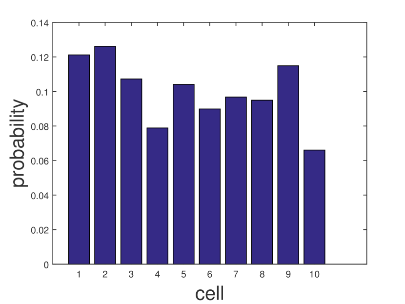
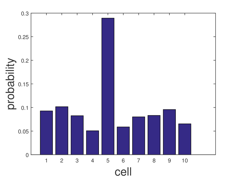
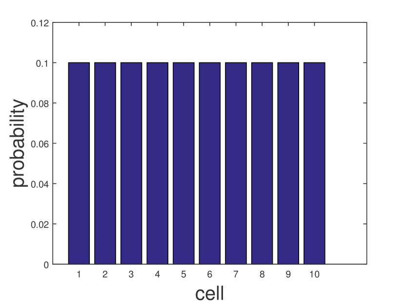
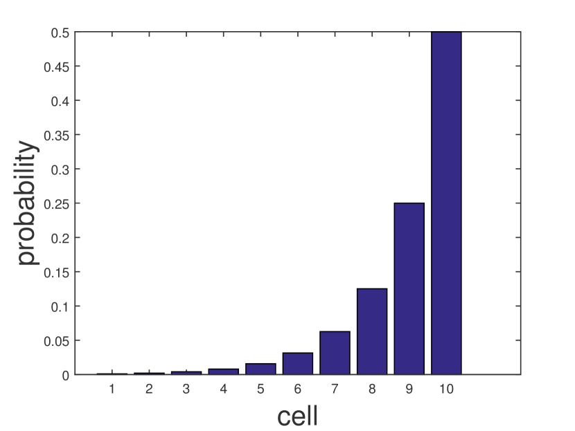
We evaluate four different mobility models for the user: (a) neither spatially nor temporally skewed mobility, represented by a MC with randomly generated transition probabilities, (b) spatially-skewed mobility, represented by a MC with a high probability of transiting into a certain cell, (c) temporally-skewed mobility, represented by a random walk with a uniform steady-state distribution, and (d) both spatially and temporally skewed mobility, represented by a random walk with a non-uniform steady-state distribution. Fig. 4 gives the steady-state distribution under each model; its deviation from the uniform distribution measures the spatial skewness. To measure temporal skewness, we evaluate the average Kullback-Leibler (KL) distance between different rows of the transition matrix (the larger, the more skewed). The distances for models (a–d) are $0.44$, $0.34$, $8.18$, and $8.48$, respectively.

(a) non-skewed

(b) spatially-skewed

(c) temporally-skewed

(d) spatially$\&$temporally-skewed

Figure 4: Steady-state distributions under various mobility models.

VII-A2 Performance under Basic Eavesdropper

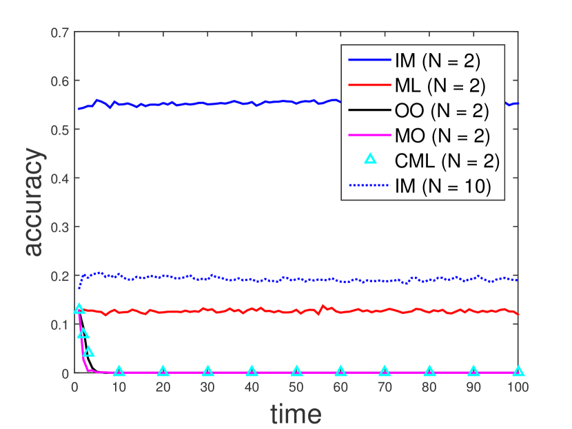
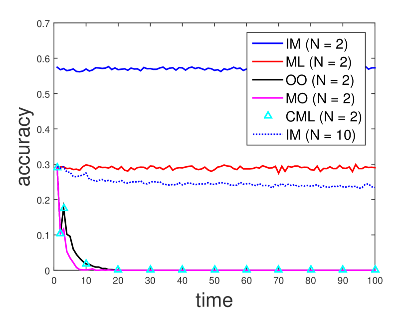
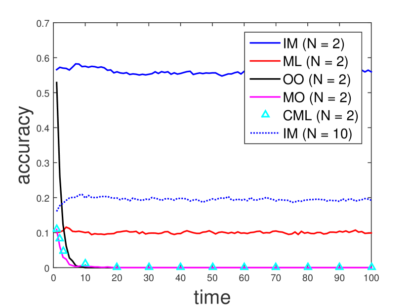
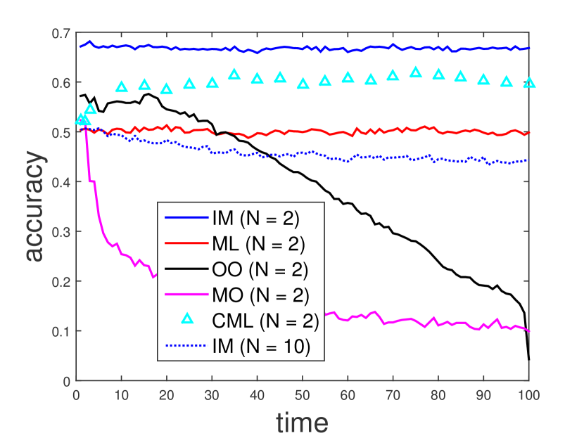
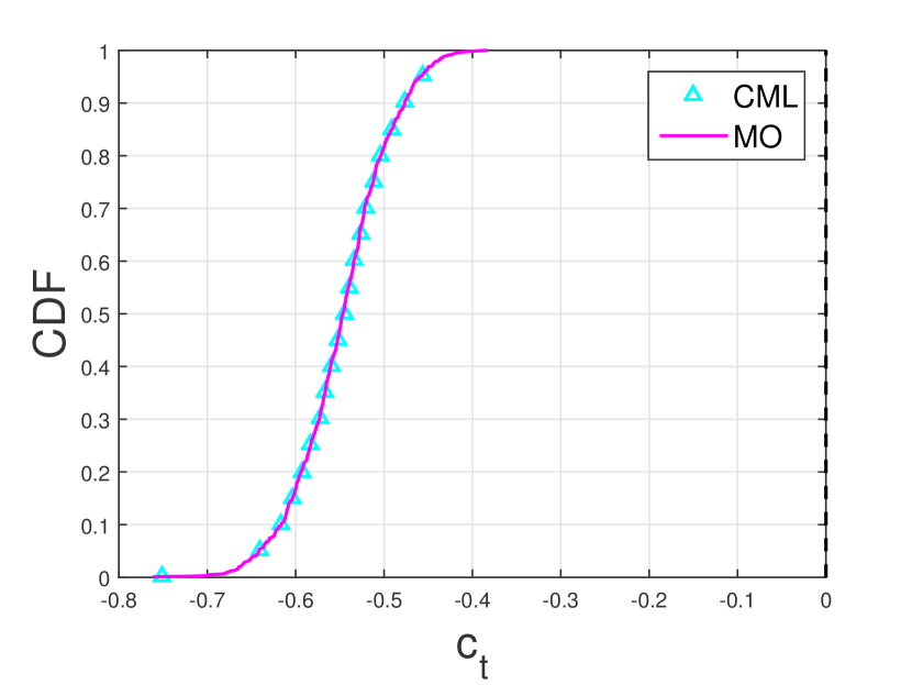
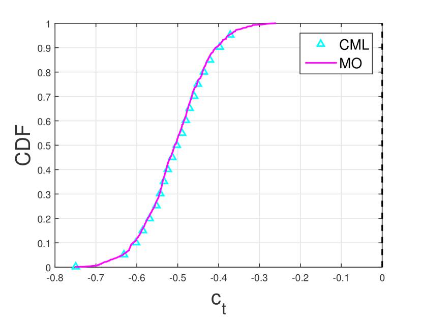
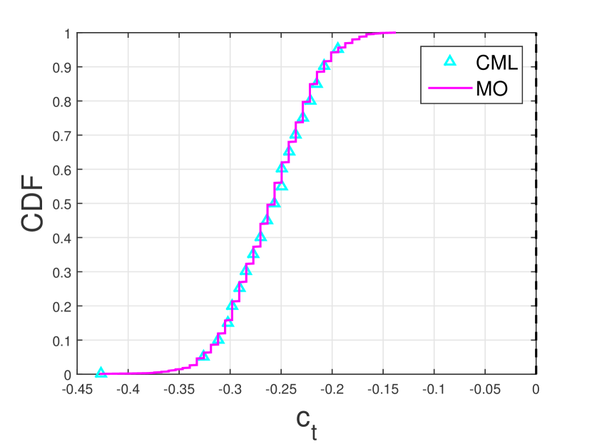
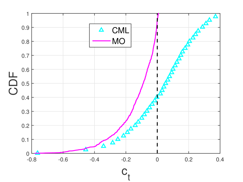
We first evaluate the performance of a basic eavesdropper using an ML detector (1); see Fig. 5. We see that: (i) while IM and ML always lead to non-zero tracking accuracy, OO and MO can drive the tracking accuracy to zero over a sufficiently long time; (ii) the more skewed the mobility model (i.e., the more predictable the user movements), the higher the tracking accuracy; (iii) while the deterministic strategies (ML, OO, MO) cannot benefit from using more chaffs, the IM strategy can use more chaffs to lower the tracking accuracy. We further simulate the auxiliary strategy CML in Section V-C and verify our analysis that the accuracy under CML/MO decays exponentially if $\mathbb{E}[c_{t}]<0$; see Fig. 6. Note that OO is designed to be optimal over $T$ slots, and is not necessarily optimal for each $t<T$. Indeed, MO achieves a lower accuracy at $t<T$ in Fig. 5 (d).

(a) non-skewed

(b) spatially-skewed

(c) temporally-skewed

(d) spatially$\&$temporally-skewed

Figure 5: Tracking accuracy of basic eavesdropper.

(a) non-skewed

(b) spatially-skewed

(c) temporally-skewed

(d) spatially$\&$temporally-skewed

Figure 6: Distribution of $c_{t}$ (defined in (19, 20)).

VII-A3 Performance under Advanced Eavesdropper

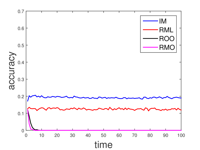
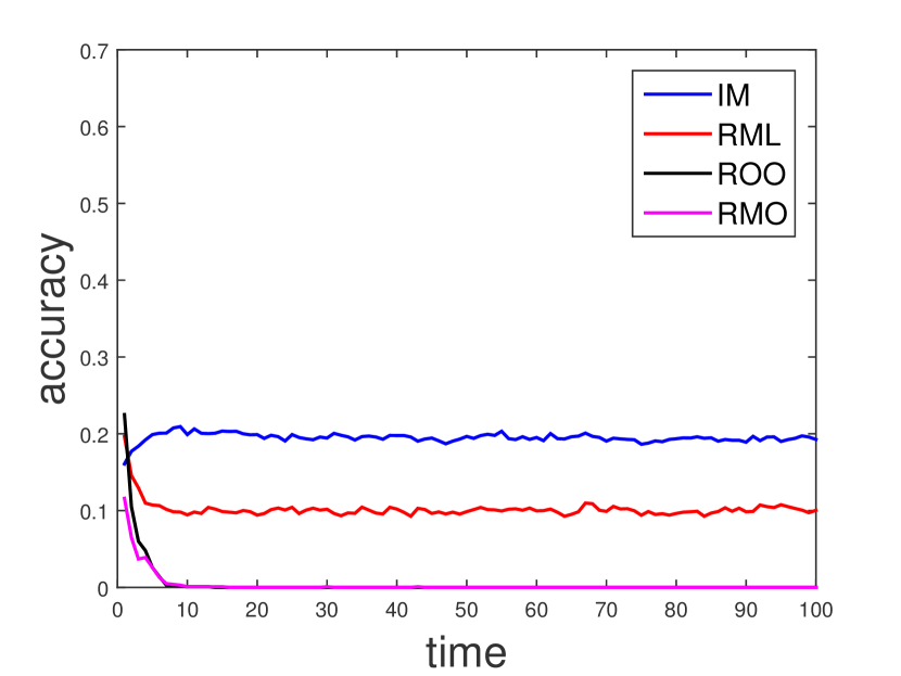
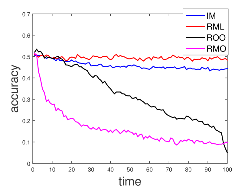
We then evaluate the performance of an advanced eavesdropper aware of the strategy. Assume that the advanced eavesdropper first filters out trajectories matching the chaff’s trajectory and then performs ML detection on the remaining trajectories. As expected, the deterministic strategies (ML, OO, MO) are ineffective against such an eavesdropper (not shown). We thus focus on the IM strategy and the robust strategies (RML, ROO, RMO) in Section VI-B; see Fig. 7. We see that by slightly perturbing the chaff’s trajectory, the robust strategies not only prevent the chaffs from being recognized by the eavesdropper but also mimic the performance of their deterministic counterparts under a basic eavesdropper.

(a) non-skewed

(b) spatially-skewed

(c) temporally-skewed

(d) spatially$\&$temporally-skewed

Figure 7: Tracking accuracy of advanced eavesdropper ($N=10$).

VII-B Trace-driven Simulations

VII-B1 Dataset

We further evaluate our solutions on real mobility traces. We use the taxi cab traces from [30], from which we extract the traces of $174$ nodes over a $100$-minute period with location updates every minute. We quantize the node locations into $959$ Voronoi cells based on cell tower locations obtained from http://www.antennasearch.com (ignoring towers within $100$ meters of others); see Fig. 8 (a). Modeling the $174$ traces as trajectories generated independently from the same MC, we compute the empirical transition matrix and the empirical steady-state distribution (Fig. 8 (b)). Clearly, this mobility model is spatially-skewed; we have verified that it is also temporally-skewed.

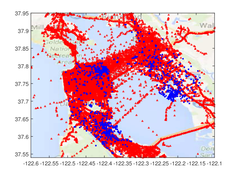
(a) $\blacktriangle$: node; $\blacksquare$: cell tower.

(b) steady-state distribution

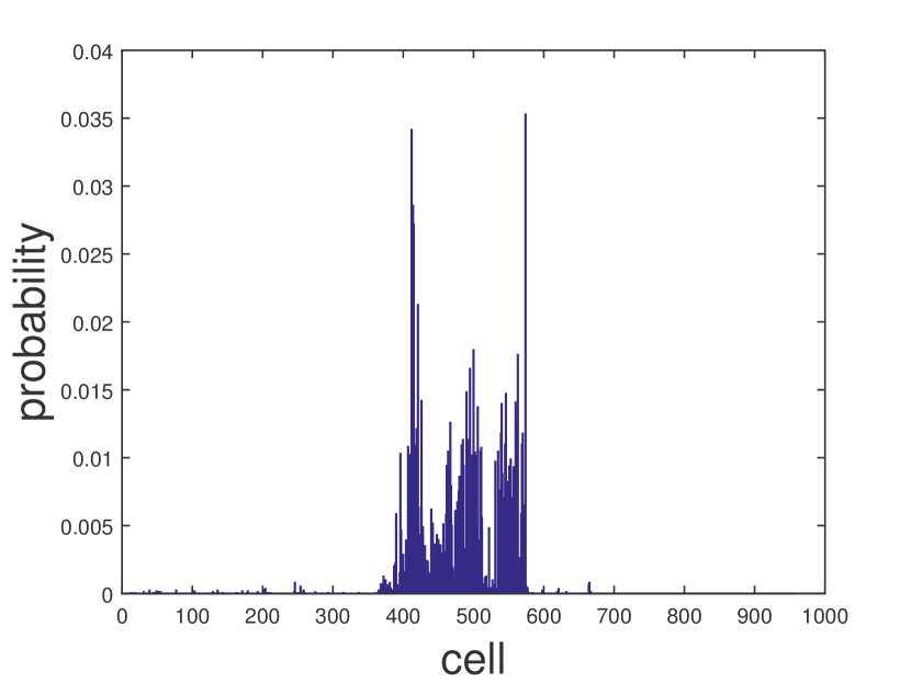
Figure 8: Cell layout and steady-state distribution.

VII-B2 Performance under Basic Eavesdropper

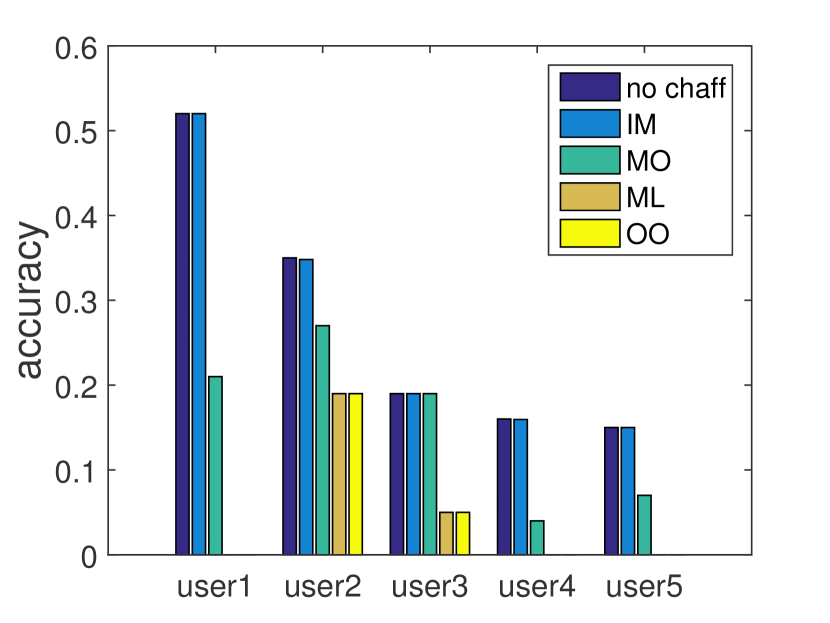
We first evaluate a basic eavesdropper running ML detection. When there is no chaff as shown in Fig. 9 (a), the eavesdropper can track a subset of users with much higher accuracy than the baseline of $1/N\approx 0.6\%$. For example, user $1$ is tracked $52\%$ of the time, and users $2,\ldots,5$ are tracked at least $15\%$ of the time. We then evaluate the accuracy in tracking the top-$K$ users ($K=5$) after adding a single chaff in Fig. 9 (b). While IM cannot help these users, ML and OO can significantly lower the tracking accuracy. Meanwhile, MO performs relatively poorly for these users, because their trajectories jointly dominate the myopic trajectory in likelihood for $55\%$ of the time, during which MO cannot alter the decision of the detector. ML and OO avoid this problem by not moving to the ML location at the beginning. Note that this limitation of MO can be overcome by using more sophisticated solvers to the MDP in Section IV-D; detailed evaluations are left to future work.

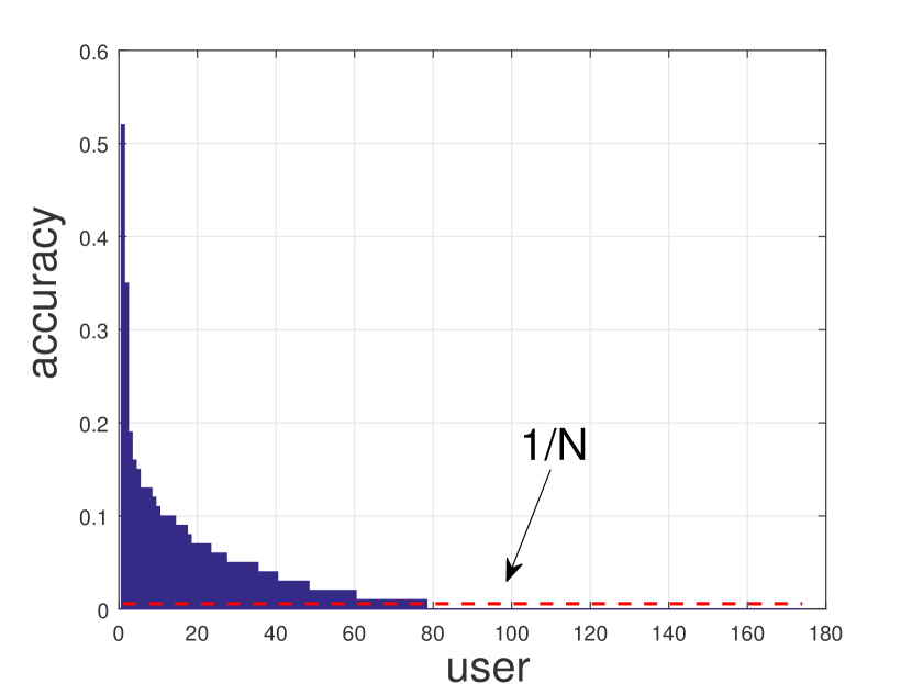
(a) no chaff

(b) a single chaff

Figure 9: Accuracy of basic eavesdropper before/after adding chaff (missing bars denote zero accuracy).

VII-B3 Performance under Advanced Eavesdropper

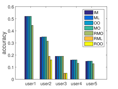
We further evaluate the performance of an advanced eavesdropper under two chaffs. As shown in Fig. 10, the original strategies (IM, ML, OO, MO) are ineffective against this eavesdropper. In contrast, the robust strategies RML and ROO can substantially reduce the tracking accuracy. Note that RMO performs poorly for reasons similar to those for MO under the basic eavesdropper.

Figure 10: Accuracy of advanced eavesdropper under $2$ chaffs.

VIII Conclusion and Discussions

We studied the problem of protecting the location privacy of a mobile user using chaff services. Assuming that a cyber eavesdropper tracks the user by performing ML detection among observed service trajectories, we examined a range of chaff control strategies, from a baseline strategy to an optimal strategy. We proved that the optimal strategy and its online variation can reduce the tracking accuracy to zero when the entropy of the user’s mobility is sufficiently high, while other straightforward strategies cannot. We further extended our strategies to improve their robustness against an advanced eavesdropper. Our evaluations highlighted the dependency of the eavesdropper’s tracking accuracy on the user’s mobility model, and verified the efficacy of our chaff-based defense mechanism in protecting the user’s location privacy, even for users with highly predictable mobility.

Discussions: We used chaff services as the defense mechanism to protect the user against untrusted MECs. Admittedly, running chaff services is expensive (see Section II-B for how we model the cost). While an ideal solution is to secure the entire system to eliminate the possibility of cyber eavesdropping, our solution provides additional protection when perfect security cannot be guaranteed (e.g., due to openness of MECs [10, 16]) or the consequence of successful eavesdropping is severe (e.g., in tactical applications). While current solutions ignore the costs of running/migrating chaff services, our formulation can be extended to include constraints on such costs, and we leave a detailed study of the cost-privacy tradeoff to future work.

Appendix

Proof of Lemma V.1

Proof.

Let $x^{*}:=\mathop{\arg\max}_{x\in\mathcal{L}}\pi(x)$. Then

$$\sum_{x\in\mathcal{L}}\pi^{2}(x)-\max_{x\in\mathcal{L}}\pi(x) =\sum_{x\neq x^{*}}\pi^{2}(x)-\pi(x^{*})(1-\pi(x^{*}))$$

$$=\sum_{x\neq x^{*}}\pi(x)(\pi(x)-\pi(x^{*}))\leq 0.$$ (37)

∎

Proof of Lemma V.2

Proof.

First, we bound $\mathbb{E}[c_{kw+i}|y_{(k-1)w+i}]$. Let $P^{t}(y|y^{\prime})$ denote the $t$-step transition probability of $\{y_{t}\}_{t=1}^{\infty}$. By definition,

$$\mathbb{E}[c_{kw+i}|y_{(k-1)w+i}] =$$

$$\sum_{y_{kw+i-1}\in\mathcal{L}^{2}}P^{w-1}(y_{kw+i-1}|y_{(k-1)w+i})g(y_{kw+i-1}),$$ (38)

and $\mathbb{E}[c_{kw+i}]$ has a similar expression with $P^{w-1}(y_{kw+i-1}|y_{(k-1)w+i})$ replaced by $\pi(y_{kw+i-1})$. Thus,

$$\Big{|}\mathbb{E}[c_{kw+i}|y_{(k-1)w+i}]-\mathbb{E}[c_{kw+i}]\Big{|} \leq$$

$$\sum_{y\in\mathcal{L}^{2}}|g(y)|\cdot\Big{|}P^{w-1}(y|y_{(k-1)w+i})-\pi(y)\Big{|}.$$ (39)

Since $w-1=t_{\mbox{\tiny mix}}(\epsilon)$, we know by the definition of mixing time that $||P^{w-1}(\cdot|y_{(k-1)w+i})-\pi||_{\mbox{\tiny TV}}\leq\epsilon$ for all $y_{(k-1)w+i}$, where $||\cdot||_{\mbox{\tiny TV}}$ denotes the total variation distance [27]. This implies that $|P^{w-1}(y|y_{(k-1)w+i})-\pi(y)|\leq\epsilon$ and $\sum_{y}|P^{w-1}(y|y_{(k-1)w+i})-\pi(y)|\leq 2\epsilon$. Thus, the righthand side of (39) is upper-bounded by both $2\epsilon\max_{y}|g(y)|$ and $\epsilon\sum_{y}|g(y)|$, i.e., by $\epsilon\delta$.

Then, by the law of total expectation, we have

$$\mathbb{E}[c_{kw+i}|c_{k^{\prime}w+i},\forall 0\leq k^{\prime}<k] =$$

$$\mathbb{E}\Big{[}\mathbb{E}[c_{kw+i}|y_{(k-1)w+i}]\Big{|}c_{k^{\prime}w+i},\forall 0\leq k^{\prime}<k\Big{]},$$ (40)

which is bounded within $[\mathbb{E}[c_{kw+i}]-\epsilon\delta,\>\mathbb{E}[c_{kw+i}]+\epsilon\delta]$ based on the above result. ∎

Proof of Lemma V.3

Proof.

Define a new random variable $Y_{t}:=X_{t}+\mu-\mathbb{E}[X_{t}|X_{1},\ldots,X_{t-1}]$. Then $\mathbb{E}[Y_{t}|Y_{1},\ldots,Y_{t-1}]=\mathbb{E}[\mathbb{E}[Y_{t}|X_{1},\ldots,X_{t-1}]|Y_{1},\ldots,Y_{t-1}]=\mu$ for all $t$. Further define $Z_{t}:=(Y_{t}-a)/(b-a+\epsilon)$. Then $Z_{t}\in[0,\>1]$ and $\mathbb{E}[Z_{t}|Z_{1},\ldots,Z_{t-1}]=(\mu-a)/(b-a+\epsilon):=\mu_{z}$.

Let $S^{y}_{n}$ denote the sum of $Y_{1},\ldots,Y_{n}$ and $S^{z}_{n}$ denote the sum of $Z_{1},\ldots,Z_{n}$. Then

$$\Pr\{S_{n}\geq n(\mu+\Delta)\} \leq\Pr\{S^{y}_{n}\geq n(\mu+\Delta)\}$$ (41)

$$=\Pr\{S^{z}_{n}\geq n\mu_{z}+{n\Delta\over b-a+\epsilon}\}$$

$$\leq e^{-2n\Delta^{2}/(b-a+\epsilon)^{2}},$$ (42)

where (41) is because $Y_{t}\geq X_{t}$, and (42) is by applying the Chernoff-Hoeffding bound [28] on $S^{z}_{n}$. ∎

Proof of Theorem V.4

Proof.

By definition of $c_{t}$, we have

$$P_{\mbox{\tiny CML}} \leq\Pr\{\sum_{t=1}^{T}c_{t}\geq 0\}\leq\Pr\{\sum_{t=2}^{T}c_{t}\geq-c_{0}\}$$

$$\leq\sum_{i=2}^{w+1}\Pr\{\sum_{k=0}^{T_{i}-1}c_{kw+i}\geq-{c_{0}\over w}\},$$ (43)

where the last step is by the union bound. Here $T_{i}:=\lfloor(T-i)/w\rfloor+1\geq T/w-1$.

By Lemma V.2, we know that $\mathbb{E}[c_{kw+i}|c_{k^{\prime}w+i},\forall 0\leq k^{\prime}<k]\in[-\mu-\epsilon\delta,\>-\mu+\epsilon\delta]$. Since $\mu-\epsilon\delta-c_{0}/(wT_{i})\geq\mu-\epsilon\delta-c_{0}/(T-w)\geq 0$, we can apply Lemma V.3 to bound $\Pr\{\sum_{k=0}^{T_{i}-1}c_{kw+i}\geq-{c_{0}\over w}\}$ by

$$\Pr\{\sum_{k=0}^{T_{i}-1}c_{kw+i}\geq-T_{i}(\mu-\epsilon\delta)+T_{i}(\mu-\epsilon\delta-{c_{0}\over wT_{i}})\}$$

$$\leq\exp\left(-2T_{i}{(\mu-\epsilon\delta-{c_{0}\over wT_{i}})^{2}\over(c_{\max}-c_{\min}+2\epsilon\delta)^{2}}\right)$$

$$\leq\exp\left(-2\Big{(}{T\over w}-1\Big{)}{(\mu-\epsilon\delta-{c_{0}\over T-w})^{2}\over(c_{\max}-c_{\min}+2\epsilon\delta)^{2}}\right).$$ (44)

Plugging (44) into (43) yields the final bound. ∎

Proof of Theorem V.5

Proof.

The proof is analogous to that of Theorem V.4. First,

$$P_{\mbox{\tiny MO}}(T) \leq\Pr\{\sum_{t=1}^{T-1}c_{t}\geq-c_{\max}\}\leq\Pr\{\sum_{t=2}^{T-1}c_{t}\geq-c_{0}-c_{\max}\}$$

$$\leq\sum_{i=2}^{w^{\prime}+1}\Pr\{\sum_{k=0}^{T_{i}-1}c_{kw^{\prime}+i}\geq-{c_{0}+c_{\max}\over w^{\prime}}\},$$ (45)

where $T_{i}:=\lfloor{T-i-1\over w^{\prime}}\rfloor+1\geq{T-w^{\prime}-1\over w^{\prime}}$.

By Lemma V.2 (with $w$ replaced by $w^{\prime}$ and $\delta$ replaced by $\delta^{\prime}$), we have that $\mathbb{E}[c_{kw^{\prime}+i}|c_{k^{\prime}w^{\prime}+i},\forall 0\leq k^{\prime}<k]\in[-\mu^{\prime}-\epsilon\delta^{\prime},\>-\mu^{\prime}+\epsilon\delta^{\prime}]$. Since $\mu^{\prime}-\epsilon\delta^{\prime}-{c_{0}+c_{\max}\over T_{i}w^{\prime}}\geq\mu^{\prime}-\epsilon\delta^{\prime}-{c_{0}+c_{\max}\over T-w^{\prime}-1}\geq 0$, we can apply Lemma V.3 to obtain

$$\Pr\{\sum_{k=0}^{T_{i}-1}c_{kw^{\prime}+i}\geq-{c_{0}+c_{\max}\over w^{\prime}}\}$$

$$\leq\exp\left(-2T_{i}{(\mu^{\prime}-\epsilon\delta^{\prime}-{c_{0}+c_{\max}\over T_{i}w^{\prime}})^{2}\over(c_{\max}-c_{\min}+2\epsilon\delta^{\prime})^{2}}\right)$$

$$\leq\exp\left(-2\Big{(}{T-w^{\prime}-1\over w^{\prime}}\Big{)}{(\mu^{\prime}-\epsilon\delta^{\prime}-{c_{0}+c_{\max}\over T-w^{\prime}-1})^{2}\over(c_{\max}-c_{\min}+2\epsilon\delta^{\prime})^{2}}\right).$$ (46)

Plugging (46) into (45) yields the final bound. ∎

Proof of Corollary V.6

Proof.

Note that Theorem V.5 holds for any value of $T$ and hence for $t=1,\ldots,T$. For $t\geq T_{0}$, the bound in Theorem V.5 applies, implying

$$P_{\mbox{\tiny MO}}(t) \leq w^{\prime}\cdot\exp\left(-2\Big{(}{t-w^{\prime}-1\over w^{\prime}}\Big{)}{(\mu^{\prime}-\epsilon\delta^{\prime}-{c_{0}+c_{\max}\over T_{0}-w^{\prime}-1})^{2}\over(c_{\max}-c_{\min}+2\epsilon\delta^{\prime})^{2}}\right)$$

$$=w^{\prime}e^{-(t-w^{\prime}-1)\alpha}.$$ (47)

For $t<T_{0}$, the bound does not apply, but we still have $P_{\mbox{\tiny MO}}(t)\leq 1$.

The overall tracking accuracy $P_{\mbox{\tiny MO}}:={1\over T}\sum_{t=1}^{T}P_{\mbox{\tiny MO}}(t)$ thus satisfies

$$P_{\mbox{\tiny MO}} \leq{1\over T}\left(T_{0}-1+\sum_{t=T_{0}}^{T}w^{\prime}e^{(w^{\prime}+1)\alpha}\cdot e^{-\alpha t}\right)$$

$$\leq{1\over T}\left(T_{0}-1+{w^{\prime}e^{\alpha(w^{\prime}+1-T_{0})}\over 1-e^{-\alpha}}\right).$$ (48)

∎

References

- [1] T. He, E. N. Ciftcioglu, S. Wang, and K. S. Chan, “Location privacy in mobile edge clouds,” in IEEE ICDCS (short paper track), June 2017, pp. 2264–2269.
- [2] M. Gruteser and D. Grunwald, “Anonymous usage of location-based services through spatial and temporal cloaking,” in ACM/USENIX MobiSys, 2003, pp. 31–42.
- [3] Y.-C. Hu and H. J. Wang, “A framework for location privacy in wireless networks,” in ACM SIGCOMM Asia Workshop, 2005.
- [4] T. Jiang, H. J. Wang, and Y.-C. Hu, “Preserving location privacy in wireless lans,” in ACM/USENIX MobiSys, 2007, pp. 246–257.
- [5] S. Wang, R. Urgaonkar, M. Zafer, T. He, K. Chan, and K. K. Leung, “Dynamic service migration in mobile edge-clouds,” in IFIP Networking, May 2015, pp. 1–9.
- [6] M. Satyanarayanan, G. Lewis, E. Morris, S. Simanta, J. Boleng, and K. Ha, “The role of cloudlets in hostile environments,” IEEE Pervasive Computing, vol. 12, no. 4, pp. 40–49, October 2013.
- [7] S. Wang, R. Urgaonkar, T. He, K. Chan, M. Zafer, and K. K. Leung, “Dynamic service placement for mobile micro-clouds with predicted future costs,” IEEE Transactions on Parallel and Distributed Systems, vol. 28, no. 4, pp. 1002–1016, April 2017.
- [8] F. Bonomi, R. Milito, J. Zhu, and S. Addepalli, “Fog computing and its role in the Internet of Things,” in The First Edition of the MCC Workshop on Mobile Cloud Computing, August 2012, pp. 13–16.
- [9] T. Taleb and A. Ksentini, “Follow me cloud: Interworking federated clouds and distributed mobile networks,” IEEE Network, vol. 27, no. 5, pp. 12–19, September 2013.
- [10] M. Satyanarayanan, R. Schuster, M. Ebling, G. Fettweis, H. Flinck, K. Joshi, and K. Sabnani, “An open ecosystem for mobile-cloud convergence,” IEEE Communications Magazine, vol. 53, no. 3, pp. 63–70, March 2015.
- [11] “Smarter wireless networks,” IBM Whitepaper No. WSW14201USEN, Febuary 2013. [Online]. Available: https://www-935.ibm.com/services/multimedia/Smarter_wireless_networks.pdf
- [12] A. Magar, “Assessing the use of tactical clouds to enhance warfighter effectiveness,” Defence Research and Development Canada Contract Report, April 2014. [Online]. Available: http://cradpdf.drdc-rddc.gc.ca/PDFS/unc198/p539325_A1b.pdf
- [13] K. Ha, Y. Abe, Z. Chen, W. He, B. Amos, P. Pillai, and M. Satyanarayanan, “Adaptive VM handoff across cloudlets,” Technical Report CMU-CS-15-113, June 2015. [Online]. Available: https://www.cs.cmu.edu/~satya/docdir/CMU-CS-15-113.pdf
- [14] T. Taleb, A. Ksentini, and P. Frangoudis, “Follow-me cloud: When cloud services follow mobile users,” accepted to IEEE Transactions on Cloud Computing, February 2016.
- [15] T. M. Takai, “Department of defense cloud computing strategy,” July 2012. [Online]. Available: http://dodcio.defense.gov/Portals/0/Documents/Cloud/DoD%20Cloud%20Computing%20Strategy%20Final%20with%20Memo%20-%20July%205%202012.pdf
- [16] R. Schuster and P. Ramchandran, “Open edge computing: From vision to reality,” OPNFV Design Summit, Berlin, Germany, June 2016.
- [17] J. Meyerowitz and R. R. Choudhury, “Hiding stars with fireworks: Location privacy through camouflage,” in ACM MobiCom, September 2009, pp. 345–356.
- [18] C.-Y. Chow, M. F. Mokbel, and X. Liu, “Spatial cloaking for anonymous location-based services in mobile peer-to-peer environments,” GeoInformatica, vol. 15, no. 2, pp. 351–380, April 2011.
- [19] A. Gkoulalas-Divanis, P. Kalnis, and V. S. Verykios, “Providing k-anonymity in location based services,” ACM SIGKDD Explorations Newsletter, vol. 12, no. 1, pp. 3–10, June 2010.
- [20] S. Jiang, N. H. Vaidya, and W. Zhao, “Power-aware traffic cover mode to prevent traffic analysis in wireless ad hoc networks,” in IEEE INFOCOM, April 2001.
- [21] T. He, L. Tong, and A. Swami, “Maximum throughput of clandestine relay,” in Allerton Conference, September 2009, pp. 1082–1089.
- [22] S. J. Stolfo, M. B. Salem, and A. D. Keromytis, “Fog computing: Mitigating insider data theft attacks in the cloud,” in IEEE Symposium on Security and Privacy Workshops, May 2012, pp. 125–128.
- [23] G. Kontaxis, M. Polychronakis, and A. D. Keromytis, “Computational decoys for cloud security,” in Secure Cloud Computing, December 2013, pp. 261–270.
- [24] A. Ksentini, T. Taleb, and M. Chen, “A Markov decision process-based service migration procedure for Follow Me cloud,” in IEEE ICC, June 2014, pp. 1350–1354.
- [25] S. Wang, R. Urgaonkar, T. He, M. Zafer, K. Chan, and K. K. Leung, “Mobility-induced service migration in mobile micro-clouds,” in IEEE MILCOM, October 2014, pp. 835–840.
- [26] S. Banerjee and D. O. Wu, “Final report from the NSF workshop on future directions in wireless networking,” National Science Foundation, November 2013.
- [27] D. A. Levin, Y. Peres, and E. L. Wilmer, Markov Chains and Mixing Times. American Mathematical Sociaty, Providence, Rhode Island, 2009.
- [28] D. Pollard, Convergence of Stochastic Processes. Springer, Berlin, Germany, 1984.
- [29] T. M. Cover and J. A. Thomas, Elements of information theory. John Wiley & Sons, 2012.
- [30] M. Piorkowski, N. Sarafijanovic-Djukic, and M. Grossglauser, “Crawdad dataset epfl/mobility (v. 2009-02-24),” February 2009. [Online]. Available: http://crawdad.org/epfl/mobility/20090224