Detailed chemical composition of classical Cepheids
in the LMC cluster NGC 1866 and in the field of the SMC

Abstract

Context. Cepheids are excellent tracers of young stellar populations. They play a crucial role in astrophysics as standard candles. The chemistry of classical Cepheids in the Milky Way is now quite well-known. Despite a much larger sample, the chemical composition of Magellanic Cepheids has been only scarcely investigated.

Aims. For the first time, we study the chemical composition of several Cepheids located in the same populous cluster: NGC 1866, in the Large Magellanic Cloud (LMC). To also investigate the chemical composition of Cepheids at lower metallicity, four targets are located in the Small Magellanic Cloud (SMC). Our sample allows us to increase the number of Cepheids with known metallicities in the LMC/SMC by 20%/25% and the number of Cepheids with detailed chemical composition in the LMC/SMC by 46%/50% .

Methods. We use canonical spectroscopic analysis to determine the chemical composition of Cepheids and provide abundances for a good number of $\alpha$, iron-peak and neutron-capture elements.

Results. We find that six Cepheids in the LMC cluster NGC 1866 have a very homogeneous chemical composition, also consistent with red giant branch (RGB) stars in the cluster. Period–age relations that include no or average rotation indicate that all the Cepheids in NGC 1866 have a similar age and therefore belong to the same stellar population. Our results are in good agreement with theoretical models accounting for luminosity and radial velocity variations. Using distances based on period-luminosity relations in the near- or mid-infrared, we investigate for the first time the metallicity distribution of the young population in the SMC in the depth direction. Preliminary results show no metallicity gradient along the SMC main body, but our sample is small and does not contain Cepheids in the inner few degrees of the SMC.

1 Introduction

Classical Cepheids are the first step on the ladder of the extragalactic distance scale. Cepheid distances were first computed from period-luminosity (PL) relations in the optical bands, but the metallicity dependence of the optical PL-relations (e.g., Romaniello et al., 2008) and the interstellar absorption led researchers to prefer period-luminosity or period-Wesenheit (PW) relations in the near-infrared (e.g., Bono et al., 2010; Feast et al., 2012; Ripepi et al., 2012; Gieren et al., 2013; Inno et al., 2013; Bhardwaj et al., 2016) where the Wesenheit index is a reddening-free quantity (Madore, 1982). In the recent years, these relations have been extended to the mid-infrared (e.g., Monson et al., 2012; Ngeow et al., 2012; Scowcroft et al., 2013; Rich et al., 2014; Ngeow et al., 2015). Most of them are tied to very accurate parallax measurements for the closest Cepheids (Benedict et al., 2007; van Leeuwen et al., 2007).

Independent distances to Cepheids can also be obtained with the Baade-Wesselink (BW) method, which combines the absolute variation of the radius of the star with the variation of its angular diameter. The former is obtained by integrating the pulsational velocity curve of the Cepheid that is derived from its radial velocity curve via the projection factor (p). The latter uses surface-brightness (SB) relations to transform variations of the color of the Cepheid to variations of its angular diameter. SB relations were first derived in the optical bands (e.g., Wesselink, 1969; Barnes & Evans, 1976) and extended to the near-infrared by Welch (1994), and Fouqué et al. (1997). Extremely accurate angular diameter variations can be obtained from interferometry (e.g., Mourard et al., 1997; Kervella et al., 2004) but this technique is currently limited to the closest Cepheids.

Published values of the $p$-factor consistently cluster around $\sim$1.3. However, the exact value of the $p$-factor and its dependence on the pulsation period remain uncertain at the level of 5-10% (Kervella et al., 2017). In a series of papers, Storm et al. (2004a, b); Gieren et al. (2005); Fouqué et al. (2007); and Storm et al. (2011a, b) found that the $p$-factor strongly depends on the period. Similar conclusions were obtained independently by Groenewegen et al. (2008, 2013). Using hydrostatic, spherically-symmetric models of stellar atmospheres, Neilson et al. (2012) indicate that the $p$-factor varies with the period, but the dependence derived is not compatible with the observational results of, e.g., Nardetto et al. (2014) and Storm et al. (2011a, b). To overcome these issues, Mérand et al. (2015) implemented a new flavor of the Baade-Wesselink method: they fit simultaneously all the photometric, interferometric and radial velocity measurements in order to obtain a global model of the stellar pulsation. Applying this method to the Cepheids for which trigonometric parallaxes are available, Breitfelder et al. (2016) found a constant value of the $p$-factor, with no dependence on the pulsation period.

Among the aforementioned studies that include LMC/SMC Cepheids, only those of Groenewegen et al. (2008, 2013) rely on abundance determinations for individual Cepheids while the others use either the (oxygen) abundances derived in nearby HII regions or a mean, global abundance for a given galaxy. Because the determination of nebular abundances is still affected by uncertainties as pointed out by Kewley et al. (2008) (but see, e.g., Pilyugin et al., 2016); and because the correlation between oxygen and iron varies from galaxy to galaxy, it is of crucial importance to have direct metallicity measurements in Cepheids. This task is now well achieved for Milky Way Cepheids (see Lemasle et al., 2007, 2008, 2013; Luck et al., 2011; Luck & Lambert, 2011; Genovali et al., 2013, 2014, 2015, and references therein). Despite the large number of Cepheids discovered in the Magellanic Clouds (3375/4630 in the LMC/SMC, respectively) by microlensing surveys such as OGLE (the Optical Gravitational Lensing Experiment Udalski et al., 2015), only a few dozens have been followed up via high-resolution spectroscopy in order to determine their metallicities (Romaniello et al., 2005, 2008) or chemical composition (Luck & Lambert, 1992; Luck et al., 1998). In this context, it is worth mentioning that by transforming a hydrodynamical model of $\delta$ Cephei into a consistent model of the same star in the LMC, Nardetto et al. (2011) found a weak dependence of the $p$-factor on metallicity (1.5% difference between LMC and Solar metallicities).

NGC 1866 is of specific interest in that respect, as it is a young (age range of 100-200 Myr), massive cluster in the outskirts of the LMC that is known to harbor a large number (23) of Cepheids (e.g., Welch & Stetson, 1993). Many studies investigated the pulsational and evolutionary properties of the intermediate-mass stars in NGC 1866 (e.g., Bono et al., 1997; Fiorentino et al., 2007; Marconi et al., 2013; Musella et al., 2016) or the multiple stellar populations in LMC clusters (Milone et al., 2017). The focus on pulsating stars in NGC 1866 is obviously driven by the need to improve the extragalactic distance scale using either period-luminosity relations or the Baade-Wesselink methods (e.g., Storm et al., 2011a, b; Molinaro et al., 2012).

It is therefore quite surprising that the chemical composition of NGC 1866 stars has been investigated only in a few high-resolution spectroscopic studies: Hill et al. (2000) analyzed a few elements in three red giant branch (RGB) stars in NGC 1866 and report [Fe/H]=$-0.50\pm 0.1$ dex. Mucciarelli et al. (2011) derived the detailed chemical composition of 14 members of NGC 1866 and of 11 additional LMC field stars. They found an average [Fe/H]=$-0.43$ dex for NGC 1866. Colucci et al. (2011, 2012a) determined the age and metallicity of NGC 1866 via high-resolution integrated light spectroscopy and extended their work to other elements in Colucci et al. (2012b). The study of Colucci et al. (2012a) also includes three stellar targets in NGC 1866 for comparison purposes, with metallicities ranging from $-0.31$ to $-0.39$ dex.

In this paper, we focus on the chemical properties of six Cepheids in NGC 1866 and four field Cepheids in the SMC, and investigate what their chemical composition tells us about the stellar populations they belong to. Our sample increases the number of Cepheids with known metallicities in the LMC/SMC by 20%/25% and the number of Cepheids with known detailed chemical composition in the LMC/SMC by 46%/50%. The Baade-Wesselink analysis will be presented in a companion paper.

2 Observations

We selected stars for which both optical & near-infrared light curves and radial velocity measurements of good quality are already available, but for which no direct determination of the metallicity exists. We selected six Cepheids in the LMC NGC 1866 cluster and four field Cepheids in the SMC. The LMC cluster stars were observed with the FLAMES/UVES high-resolution spectrograph (Pasquini et al., 2002) while the SMC field stars were observed with the UVES high-resolution spectrograph (Dekker et al., 2000). We used the red arm (CD #3) standard template centered on 580 nm which offers a resolution of 47 000 and covers the 476–684 nm wavelength range with a 5 nm gap around the central wavelength. We used the ESO reflex pipeline (Freudling et al., 2013) to perform the basic data reduction of the spectra. The heliocentric corrections of the radial velocities were computed with the IRAF task rvcorrect. The observing log is listed in Table 1. For the FLAMES/UVES sample, the weather conditions deteriorated during the night. We therefore analyzed only the first three spectra of a series of six for each star, as they reached a higher S/N. The S/N values are listed in Table 3.

The phases were computed by adopting the period and the epoch of maximum light from OGLE IV (Udalski et al., 2015) as a zero point reference, except for HV 12202 for which no OGLE IV data are available. For this star, we used the values provided by Molinaro et al. (2012). The computations were made using heliocentric Julian dates (HJD), i. e., 0.5 days were added to the modified Julian dates (MJD) and the light travel time between the Earth and the Sun was taken into account. The HJDs were double-checked using the IRAF task rvcorrect.

Table 1: Observing log. The first six lines are spectra taken with the FLAMES/UVES multi-object spectrograph. The other spectra were taken with the UVES spectrograph.

Target	Date	MJD	Airmass	Exp time
			(start)	(s)
NGC 1866	2008-12-06T00:35:23.385	54806.02457622	1.848	4800
NGC 1866	2008-12-06T01:56:13.752	54806.08071473	1.541	4800
NGC 1866	2008-12-06T03:17:03.638	54806.13684767	1.381	4800
NGC 1866	2008-12-06T04:50:18.350	54806.20160128	1.320	4800
NGC 1866	2008-12-06T06:11:08.646	54806.25773897	1.358	4800
NGC 1866	2008-12-06T07:31:58.631	54806.31387305	1.490	3600
HV 822	2008-11-15T00:57:58.745	54785.04026326	1.531	1000
	2008-11-15T01:15:28.075	54785.05240828	1.523	1000
	2008-11-15T01:32:57.446	54785.06455378	1.519	1000
HV 1328	2008-11-15T00:11:13.084	54785.00779033	1.569	800
	2008-11-15T00:25:22.587	54785.01762254	1.556	800
	2008-11-15T00:39:31.570	54785.02744873	1.545	800
HV 1333	2008-11-15T01:53:56.155	54785.07912217	1.531	1200
	2008-11-15T02:14:45.620	54785.09358357	1.537	1200
	2008-11-15T02:35:34.996	54785.10804394	1.547	1200
HV 1335	2008-11-15T03:03:49.091	54785.12765152	1.569	1300
	2008-11-15T03:26:18.517	54785.14326987	1.594	1300
	2008-11-15T03:48:48.862	54785.15889887	1.625	1300

3 Chemical abundances

3.1 Data analysis

In our spectra, we measured the equivalent widths of the absorption lines with DAOSPEC (Stetson & Pancino, 2008): DAOSPEC fits lines with saturated Gaussians and all the lines detected are cross-correlated with a list of lines provided by the user. For each individual measurement of an equivalent width (EW), DAOSPEC provides the standard error $\sigma_{EW}$ on the measurement and a quality parameter Q that becomes higher in the regions where the quality of the spectrum decreases or for strong lines that deviate from a Gaussian profile. We selected only lines with $\sigma_{EW}$ $\leq$ 10 % and Q $\leq$ 1.25. For both the determination of the atmospheric parameters and the computation of the abundances, we considered only the lines with 20 $\leq$ EW $\leq$ 130 mÅ.

The equivalent width method was favoured as it enables a more homogeneous continuum placement, especially for spectra with a relatively low S/N like ours (see examples in Fig.1). The hyperfine structure can therefore not be taken into account. Current studies indicate that the effects of hyperfine structure splitting (hfs) are negligible or small for Y, Zr, Nd, and Eu in Cepheids (da Silva et al., 2016), but not for Mn (Lemasle et al., in prep) or to a lesser extent La (da Silva et al., 2016). A more detailed discussion about the hfs is provided in Sect 4.

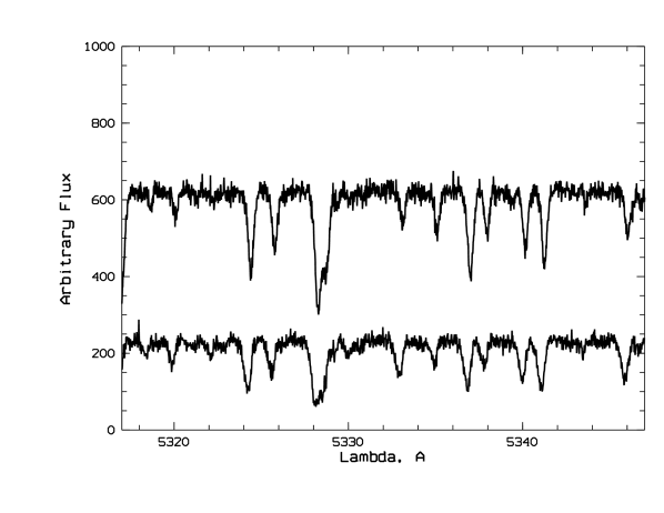
Figure 1: Excerpts of spectra covering the 5317–5347 Å range. Top: HV1328 (SMC) at MJD=54785.01762254 (S/N$\approx$20). Bottom: HV12198 (NGC 1866) at 54806.13684767 (S/N$\approx$30).

3.2 Radial velocities

For the NGC 1866 sample, the accuracy of the radial velocity determined by DAOSPEC is in general better than $\pm$2 km s^-1, with a mean error in the individual velocities measurement of 1.157 km s^-1. Thanks to a higher S/N, the radial velocities for the SMC sample are even more accurate, with a mean error of 0.804 km s^-1. Our measurements are listed in Table 2. Comments in footnotes come from the OGLE-III database (Soszyński et al., 2010). Note that in both cases the radial velocities obtained from the lower (L) and the upper (U) chip of the UVES red arm are in excellent agreement. The averaged radial velocities and the heliocentric corrections (computed with the IRAF task rvcorrect, with a negligible uncertainty of $\approx$0.005 km s^-1) are also listed in Table 2.

Table 2: Radial velocities for our targets in the LMC cluster NGC 1866 and in the field of the SMC. The radial velocities derived for the lower (L) and upper (U) chips of the UVES red arm are listed in cols. 4 and 5. The averaged values are listed in col. 6, the barycentric corrections in col.7 and the final values for the radial velocity (after correction) in col. 8.

Targets in the LMC cluster NGC 1866
Target	Period (P)	Phase $\phi$	VrL	VrU	Vr (averaged)	Heliocentric correction	Vr corrected
	(d)		(km s-1)	(km s-1)	(km s-1)	(km s-1)	(km s-1)
HV 12197	3.1437642	0.081	283.399$\pm$1.919	282.260$\pm$3.202	283.098$\pm$1.646	-2.205	280.893$\pm$1.646
		0.099	284.238$\pm$1.390	284.180$\pm$1.641	284.214$\pm$1.061	-2.242	281.972$\pm$1.061
		0.117	285.289$\pm$1.567	284.997$\pm$1.378	285.124$\pm$1.035	-2.294	282.830$\pm$1.035
HV 12198	3.5227781	0.643	315.940$\pm$1.384	315.921$\pm$1.552	315.932$\pm$1.033	-2.190	313.742$\pm$1.033
		0.659	316.662$\pm$1.031	316.566$\pm$1.332	316.626$\pm$0.815	-2.227	314.399$\pm$0.815
		0.675	316.960$\pm$1.305	316.943$\pm$1.097	316.950$\pm$0.840	-2.279	314.671$\pm$0.840
HV 12199	2.6391571	0.928	289.626$\pm$2.129	289.346$\pm$4.279	289.570$\pm$1.906	-2.199	287.371$\pm$1.906
		0.949	284.720$\pm$1.187	284.655$\pm$2.177	284.705$\pm$1.042	-2.236	282.469$\pm$1.042
		0.970	281.507$\pm$1.528	281.312$\pm$1.867	281.429$\pm$1.182	-2.288	279.141$\pm$1.182
HV 12202	3.101207	0.807	319.318$\pm$2.632	318.444$\pm$4.291	319.079$\pm$2.244	-2.180	316.899$\pm$2.244
		0.825	316.907$\pm$2.040	316.018$\pm$2.053	316.465$\pm$1.447	-2.217	314.248$\pm$1.447
		0.843	313.635$\pm$1.472	312.713$\pm$3.442	313.492$\pm$1.353	-2.269	311.223$\pm$1.353
HV 12203	2.9541342	0.765	323.664$\pm$1.902	323.307$\pm$2.098	323.503$\pm$1.409	-2.180	321.323$\pm$1.409
		0.784	322.905$\pm$1.775	322.400$\pm$1.448	322.602$\pm$1.122	-2.217	320.385$\pm$1.122
		0.803	320.983$\pm$1.407	321.260$\pm$1.702	321.095$\pm$1.084	-2.269	318.826$\pm$1.084
HV 12204	3.4387315	0.519	292.454$\pm$0.524	292.107$\pm$0.955	292.374$\pm$0.459	-2.163	290.211$\pm$0.459
		0.535	293.664$\pm$0.919	293.164$\pm$0.751	293.364$\pm$0.582	-2.200	291.164$\pm$0.582
		0.551	294.177$\pm$0.713	294.166$\pm$0.895	294.173$\pm$0.558	-2.252	291.921$\pm$0.558
Targets in the SMC
HV 822	16.7419693	0.998	101.288$\pm$1.736	101.438$\pm$2.309	101.342$\pm$1.388	-12.692	88.650$\pm$1.388
		0.999	101.143$\pm$1.931	101.027$\pm$1.672	101.077$\pm$1.264	-12.701	88.376$\pm$1.264
		0.999	101.450$\pm$0.939	100.845$\pm$1.543	101.286$\pm$0.802	-12.709	88.577$\pm$0.802
HV 1328	15.8377104	0.883	121.800$\pm$1.013	121.771$\pm$1.605	121.792$\pm$0.857	-12.808	108.984$\pm$0.857
		0.884	121.592$\pm$0.626	121.509$\pm$0.615	121.550$\pm$0.439	-12.814	108.736$\pm$0.439
		0.884	121.402$\pm$1.069	121.716$\pm$0.876	121.590$\pm$0.678	-12.821	108.769$\pm$0.678
HV 1333	16.2961015	0.659	179.553$\pm$1.333	179.786$\pm$0.735	179.732$\pm$0.644	-12.742	166.990$\pm$0.644
		0.660	179.816$\pm$1.267	179.909$\pm$0.930	179.876$\pm$0.750	-12.752	167.124$\pm$0.750
		0.661	179.486$\pm$1.555	179.972$\pm$0.827	179.865$\pm$0.730	-12.761	167.104$\pm$0.730
HV 1335	14.3813503	0.318	163.310$\pm$0.763	163.376$\pm$1.360	163.326$\pm$0.665	-12.750	150.576$\pm$0.665
		0.319	162.985$\pm$1.154	163.194$\pm$1.102	163.094$\pm$0.797	-12.760	150.334$\pm$0.797
		0.320	163.352$\pm$1.466	163.198$\pm$0.877	163.239$\pm$0.753	-12.769	150.470$\pm$0.753

Because this was one of our target selection criteria, there is an extensive amount of radial velocity data available for the Cepheids in our sample. From these data it was possible to ascertain that our NGC 1866 Cepheids are indeed cluster members. Excluding variable stars, Mucciarelli et al. (2011) report an average heliocentric velocity of v=298.5$\pm$0.4 km s^-1 with a dispersion of $\sigma$=1.6 km s^-1. For both the LMC and SMC targets our radial velocity measurements are in excellent agreement with the expected values at the given pulsation phase obtained from the radial velocity curves published in the literature (Welch et al., 1991; Storm et al., 2004a, 2005; Molinaro et al., 2012; Marconi et al., 2013, 2017).

Systematic shifts between different samples are generally attributed to the orbital motion in a binary system. Two stars in our sample (HV 12202 and HV 12204) were identified as spectroscopic binaries (Welch et al., 1991; Storm et al., 2005). As far as HV 12202 is concerned, our measurements are in good agreement with all the data compiled by Storm et al. (2005) except for their CTIO data and the latest part of the Welch et al. (1991) data, and therefore support the shifts of +18 km s^-1 (respectively +21 km s^-1) applied to these datasets in order to provide an homogeneous radial velocity curve. For the same purpose, the latest data from Welch et al. (1991) had to be shifted by +7 km s^-1 and our measurements should be shifted by $\approx$ +15 km s^-1 in the case of HV 12204. Binarity is a common feature for Milky Way Cepheids (more than 50% of them are binaries, see Szabados, 2003), but there is a strong observational bias with distance and indeed the number of known binaries is much lower for the farther, fainter Cepheids in the Magellanic Clouds (Szabados & Nehéz, 2012). It should be noted that Anderson (2014) found modulations in the radial velocity curves of four Galactic Cepheids. However, the order of magnitude of the effect ranges from several hundred m s^-1 to a few km s^-1 and cannot account for the differences reported here in the case of HV 12202 and HV 12204.

3.3 Atmospheric parameters

As Cepheids are variable stars, simultaneous photometric and spectroscopic observations are in general not available and the atmospheric parameters are usually derived from the spectra only. Kovtyukh & Gorlova (2000) have developed an accurate method to derive the effective temperature $T_{\rm eff}$ from the depth ratio of carefully chosen pairs of lines that have been used extensively in Cepheids studies (Andrievsky et al., 2002a; Luck & Lambert, 2011).

As the red CCD detector of UVES is made of two chips side by side (lower: L; upper: U), there is a gap of $\approx$ 50 Å around the central wavelength (580 nm in our case) and we could not use the lines falling in this spectral domain. Moreover, the line depth ratios have been calibrated for Milky Way Cepheids that are more metal-rich than the Magellanic Cepheids (especially in the case of the SMC). It also turns out that several stars in our sample were observed at a phase where they reach higher $T_{\rm eff}$ ($>$6000 K) during the pulsation cycle. The combination of a high $T_{\rm eff}$ and a rather low metallicity made it very challenging to measure the depth of some lines, and in particular the weak line of the pairs. As a result, we could only use a limited number of line depth ratios (typically 5–10 out of 32) to determine $T_{\rm eff}$. Moreover, for two stars (HV 12199 and HV 822), we were unable to determine $T_{\rm eff}$ from the line depth ratio as their temperature ($>$6400 K) at the time of the observations fell above the range of temperatures where most ratios are calibrated .

To ensure the determination of $T_{\rm eff}$, we double-checked that lines with both high and low $\chi_{\rm ex}$ values properly fit the curve of growth (See Appendix D) and that the Fe I abundances are independent from the excitation potential of the lines. In a canonical spectroscopic analysis, we determined the surface gravity $log\leavevmode\nobreak\ g$ and the microturbulent velocity V_t by imposing that the ionization balance between Fe I and Fe II is satisfied and that the Fe I abundance is independent from the EW of the lines. On average we have at our disposal 42 Fe I/7 Fe II lines in the NGC 1866 Cepheids and 42 Fe I/11 Fe II lines in the SMC Cepheids. We note that the adopted $T_{\rm eff}$ values are in general in very good agreement with those derived from the line depth ratios. The atmospheric parameters are listed in Table 3.

As mentioned above, the Cepheids in our sample have rather high temperatures, two of them hot enough at the phase of the observations to prevent the use of line depth ratios to determine their temperature. It has been noted before (Brocato et al., 2004) that these stars are located in the color-magnitude diagram at the hot tip of the so-called ”blue nose” experienced by core He-burning supergiants. During this evolutionary stage they cross the instability strip and start pulsating.

As we impose the ionization balance between Fe I and Fe II to derive $log\leavevmode\nobreak\ g$, NLTE effects affecting primarily Fe I could hamper an accurate determination of $log\leavevmode\nobreak\ g$ (Luck & Lambert, 1985). There is currently no extensive study of NLTE effects in Cepheids, although NLTE abundances have been derived for some individual elements like O (Korotin et al., 2014, and references therein) or Ba (Andrievsky et al., 2014, and references therein). It is beyond the scope of this paper to provide a full discussion of NLTE effects in Cepheids, and we refer the reader to the discussion in e.g., Kovtyukh & Andrievsky (1999) or Yong et al. (2006). Several arguments have been brought forward to support the fact that NLTE effects may be limited in Cepheids. For instance, Andrievsky et al. (2005) followed several Cepheids with 3d$<$P$<$6d throughout the entire period and found identical [Fe/H] and abundances ratios (within the uncertainties), although $T_{\rm eff}$ varies by $\approx$ 1000 K (the same holds for Cepheids with different period ranges studied in this series of papers). Also Yong et al. (2006) found a mean difference [TiI/Fe]–[TiII/Fe]=0.07$\pm$0.02 ($\sigma$=0.11). As this difference falls within the measurement uncertainties, they concluded that the values of $log\leavevmode\nobreak\ g$ obtained via the ionization equilibrium of FeI/FeII are satisfactory. All these arguments point toward the fact that a canonical spectroscopic analysis provides consistent, reliable results. However, the aforementioned studies deal with Milky Way Cepheids. As Magellanic Cepheids are slightly more metal-poor, NLTE effects should be a bit more pronounced than in the Galactic ones. In a study of 9 LMC F supergiants, Hill et al. (1995) introduced an overionization law and obtained higher (+0.6 dex) spectroscopic gravities that are in good agreement with those derived from photometry. They note that [Fe/H] becomes only +0.1 dex higher than in the LTE case and that the global abundance pattern remains unchanged, as already reported by, e.g., Spite et al. (1989).

3.4 Comparison with models

Marconi et al. (2013) have used non-linear convective pulsation models in order to reproduce simultaneously the lightcurves in several photometric bands and the radial velocity curves of a few Cepheids in NGC 1866. For HV 12197 they reached a good agreement between theory and observations and report a mean $T_{\rm eff}$ of 5850 K. They also plotted the temperature predicted by the model and for the phases 0.08–0.12 they found $T_{\rm eff}$ of the order of 6300 K and slightly below (their Fig. 8, bottom panel), in quite good agreement with our measurements that fall around 6150 K. For HV 12199, they report a mean $T_{\rm eff}$ of 6125 K but had to modify notably the projection factor to reach the best match with the radial velocity curve. They also mention that using the lightcurves only would lead to a hotter star (¡ $T_{\rm eff}$ ¿ = 6200 K), but in this case an even lower (and unrealistic) value would be required for the projection factor in order to fit the radial velocity curve. The $T_{\rm eff}$ curve for HV 12199 (their Fig. 8, top panel) in the phases 0.93–0.97 shows a rapid rise of the temperature and the corresponding $T_{\rm eff}$ value of $\approx$ 6250–6300 K, somewhat below the values around 6600 K we determined for $T_{\rm eff}$.

3.5 Abundance determinations

Our abundance analysis is based on equivalent widths measured with DAOSPEC (see Sect. 3.1). We derived the abundances of 16 elements (several of them in two ionization states) for which absorption lines could be measured in the spectral domain covered by the UVES red arm (CD  #3, 580 nm) standard template. In a few cases we updated the linelists of Genovali et al. (2013) and Lemasle et al. (2013) with oscillator strengths and excitation potentials from recent releases of the Vienna Atomic Lines Database (VALD, Kupka et al., 1999, and references therein) and from the Gaia-ESO survey linelist (Heiter et al., 2015). We took the values tabulated by Anders & Grevesse (1989) as Solar references, except for Fe and Ti for which we used $log\leavevmode\nobreak\ \epsilon_{Fe}$=7.48 and $log\leavevmode\nobreak\ \epsilon_{Ti}$=5.02. We used MARCS (1D LTE spherical) atmosphere models (Gustafsson et al., 2008) covering the parameter space of Magellanic Clouds Cepheids. Abundances were computed with calrai, a LTE spectrum synthesis code originally developed by Spite (1967) and continuously updated since then. For a given element, the abundance derived from a single spectrum is estimated as the mean value of the abundances determined for each individual line of this element. The final abundance of a star is then obtained by computing the weighted mean (and standard deviation) for the three spectra analyzed, where the weight is the number of lines of a given element measured in each spectrum.

Table 3: Coordinates, properties and atmospheric parameters for the Cepheids in our sample. V magnitudes and periods are from OGLE IV, except for HV12202, for which they have been found in Molinaro et al. (2012) and Musella et al. (2016). Col. 7 refers to the $T_{\rm eff}$ derived from the line depth ratio method (LDR, Kovtyukh & Gorlova, 2000) while col. 8 is the $T_{\rm eff}$ derived from the excitation equilibrium. The last column lists the S/N around 5228 and 5928 Å respectively.

Targets in the LMC cluster NGC 1866
Cepheid	RA (J2000)	Dec (J2000)	V	P	$\phi$	$T_{\rm eff}$ (LDR)	$T_{\rm eff}$	$log\leavevmode\nobreak\ g$	Vt	[Fe/H]	S/N
	(dms)	(dms)	(mag)	(d)		(K)	(K)	(dex)	(km s-1)	(dex)	(5228/5928Å)
HV 12197	05 13 13.0	-65 30 48	16.116	3.1437642	0.081	6060$\pm$ 97 (3)	6150	1.5	3.1	-0.35	16/15
				3.1437642	0.099		6150	1.5	3.2	-0.35	28/27
				3.1437642	0.117		6100	1.5	3.1	-0.35	27/25
HV 12198	05 13 26.7	-65 27 05	15.970	3.5227781	0.643	5634$\pm$ 85 (6)	5625	1.4	3.4	-0.35	13/19
				3.5227781	0.659		5625	1.5	3.6	-0.35	20/26
				3.5227781	0.675		5625	1.4	3.6	-0.35	21/23
HV 12199	05 13 19.0	-65 29 30	16.283	2.6391571	0.928	–	6550	2.2	3.2	-0.30	15/14
				2.6391571	0.949		6600	2.1	3.0	-0.30	29/31
				2.6391571	0.970		6650	2.0	3.1	-0.35	26/32
HV 12202	05 13 39.0	-65 29 00	16.08	3.101207	0.807	5712$\pm$100 (6)	5775	1.6	3.1	-0.40	17/14
				3.101207	0.825		5900	1.6	3.1	-0.40	20/25
				3.101207	0.843		5900	1.5	2.9	-0.40	20/24
HV 12203	05 13 40.0	-65 29 36	16.146	2.9541342	0.765	5856$\pm$117 (9)	5850	1.7	3.5	-0.35	16/19
				2.9541342	0.784		5800	1.2	3.3	-0.35	17/26
				2.9541342	0.803		5800	1.6	3.4	-0.35	19/24
HV 12204	05 13 58.0	-65 28 48	15.715	3.4387315	0.519	5727$\pm$ 98 (11)	5700	1.2	2.8	-0.35	19/23
				3.4387315	0.535		5725	1.3	2.9	-0.35	22/31
				3.4387315	0.551		5700	1.2	2.9	-0.35	21/28
Targets in the SMC
HV 822	00 41 55.5	-73 32 23	14.524	16.7419693	0.998	–	6400	1.8	2.7	-0.75	33/48
				16.7419693	0.999		6400	1.8	2.7	-0.75	41/46
				16.7419693	0.999		6400	1.8	2.7	-0.75	35/42
HV 1328	00 32 54.9	-73 49 19	14.115	15.8377104	0.883	6325$\pm$ 98 (5)	6100	1.9	2.6	-0.60	26/37
				15.8377104	0.884		6100	1.9	2.6	-0.60	31/37
				15.8377104	0.884		6100	1.9	2.6	-0.60	29/40
HV 1333	00 36 03.5	-73 55 58	14.729	16.2961015	0.659	5192$\pm$102 (8)	5175	0.4	3.2	-0.90	18/26
				16.2961015	0.660		5200	0.4	2.8	-0.80	19/25
				16.2961015	0.661		5175	0.4	3.2	-0.90	16/30
HV 1335	00 36 55.7	-73 56 28	14.762	14.3813503	0.318	5566$\pm$156 (6)	5600	0.6	2.6	-0.80	25/29
				14.3813503	0.319		5675	0.8	2.6	-0.75	28/29
				14.3813503	0.320		5600	0.6	2.7	-0.80	25/29

3.6 Abundances

We provide the abundances of one light element (Na), several $\alpha$-elements (Mg, Si, S, Ca, Ti), iron-peak elements (Sc, Cr, Mn, Fe, Ni), and neutron capture elements (Y, Zr, La, Nd, Eu). As already mentioned, we analyzed three individual (back to back) spectra for each star and the abundances derived are in most cases in excellent agreement. As expected, the size of the error bars is correlated to the number of lines analyzed. In contrast to our Cepheid studies in the Milky Way, where Si comes second after iron for the number of lines measured, the UVES red arm (CD #3, 580 nm) spectral domain contains only a few Si lines with sufficient quality but a larger number of Ca lines and indeed 9–11 calcium lines were usually measured in our spectra. The individual abundances (per spectrum) are listed in Tables 7–12 for the NGC 1866 Cepheids and in Tables 13–16 for the SMC Cepheids. The last two columns of these tables list the weighted means and standard deviations, adopted as the chemical composition of the star in the rest of the paper.

Molinaro et al. (2012) provide the metallicities for three Cepheids in NGC 1866, analyzed in the same way as the stars in Mucciarelli et al. (2011). Two of Molinaro et al. (2012) Cepheids are also included in our sample, namely HV 12197 and HV 12199: taking into account a tiny difference (0.02 dex) in the solar reference value for [Fe/H], the results agree very well: they report [Fe/H]=$-0.39\pm 0.05$ for HV 12197 while we found $-0.33\pm 0.07$ dex, and [Fe/H]=$-0.38\pm 0.06$ for HV 12199 while we found $-0.31\pm 0.05$.

For a good number of our spectra, several elements (Si, Ti, Cr) could be measured in two ionization states, in addition to the usual Fe I / Fe II. When the ionization equilibrium is reached for iron, it is usually also reached for the other elements as the abundances derived from the neutral and ionized species agree within the error bars, thus reinforcing our confidence in our atmospheric parameters, in particular $log\leavevmode\nobreak\ g$. In order to quantify how the results are affected by uncertainties in the atmospheric parameters, we computed the abundances with over- or underestimated values of $T_{\rm eff}$($\pm$150 K), $log\leavevmode\nobreak\ g$($\pm$0.3 dex), V_t($\pm$0.5 km s^-1) for two spectra at different $T_{\rm eff}$. Uncertainties in [Fe/H] leave the abundances unchanged and are therefore not considered in this exercise. The sum in quadrature of the differences in the computed abundances is adopted as the uncertainty in the abundances due to the uncertainties in the atmosphere parameters. The resulting values are listed in Table 4.

Table 4: Uncertainties in the final abundances due to uncertainties in the atmospheric parameters. Cols. 2, 3, 4 indicate respectively how the abundances are modified (mean values) when they are computed with over- or underestimated values of $T_{\rm eff}$($\pm$150 K), $log\leavevmode\nobreak\ g$($\pm$0.3 dex), or V_t($\pm$0.5 dex). The sum in quadrature of the differences is adopted as the uncertainty in the abundances due to the uncertainties in the atmosphere parameters

Error budget for HV 12198, $\phi$=0.675 (MJD=54806.13684767)
Element	$\Delta$$T_{\rm eff}$	$\Delta$$log\leavevmode\nobreak\ g$	$\Delta$Vt	Quadratic
	($\pm$ 150 K)	($\pm$ 0.3 dex)	($\pm$ 0.5 km s-1)	sum
	(dex)	(dex)	(dex)	(dex)
[NaI/H]	0.08	0.00	0.03	0.09
[MgI/H]	0.14	0.00	0.08	0.16
[SiI/H]	0.07	0.01	0.03	0.07
[SiII/H]	0.12	0.12	0.11	0.19
[SI/H]	0.07	0.08	0.04	0.11
[CaI/H]	0.10	0.00	0.06	0.12
[ScII/H]	0.03	0.12	0.08	0.15
[TiI/H]	0.15	0.00	0.03	0.15
[TiII/H]	0.02	0.12	0.02	0.12
[CrII/H]	0.02	0.11	0.07	0.13
[MnI/H]	0.12	0.00	0.03	0.12
[FeI/H]	0.13	0.00	0.05	0.13
[FeII/H]	0.01	0.12	0.05	0.13
[NiI/H]	0.13	0.00	0.04	0.13
[YII/H]	0.04	0.12	0.05	0.13
[ZrII/H]	0.03	0.11	0.03	0.12
[LaII/H]	0.07	0.12	0.04	0.14
[NdII/H]	0.07	0.22	0.05	0.23
[EuII/H]	0.04	0.12	0.02	0.12
Error budget for HV 1328, $\phi$=0.884 (MJD=54785.02744873)
Element	$\Delta$$T_{\rm eff}$	$\Delta$$log\leavevmode\nobreak\ g$	$\Delta$Vt	Quadratic
	($\pm$ 150 K)	($\pm$ 0.3 dex)	($\pm$ 0.5 km s-1)	sum
	(dex)	(dex)	(dex)	(dex)
[NaI/H]	0.10	0.04	0.02	0.11
[MgI/H]	0.11	0.05	0.02	0.12
[SiI/H]	0.18	0.07	0.02	0.19
[CaI/H]	0.13	0.06	0.04	0.15
[ScII/H]	0.28	0.10	0.06	0.30
[TiI/H]	0.09	0.11	0.03	0.15
[TiII/H]	0.12	0.03	0.07	0.14
[CrI/H]	0.13	0.05	0.07	0.15
[CrII/H]	0.10	0.07	0.06	0.13
[FeI/H]	0.11	0.06	0.08	0.15
[FeII/H]	0.22	0.13	0.09	0.26
[NiI/H]	0.09	0.13	0.05	0.16
[YII/H]	0.07	0.08	0.03	0.11
[ZrII/H]	0.31	0.12	0.02	0.33
[LaII/H]	0.13	0.05	0.03	0.14
[NdII/H]	0.10	0.15	0.03	0.18
[EuII/H]	0.28	0.08	0.03	0.29

For the stars in our sample, NLTE effects are negligible for Na ($\leq$ 0.1 dex) as computed by Lind et al. (2011) for a range of atmospheric parameters including yellow supergiants and by Takeda et al. (2013) for Cepheids. Using DAOSPEC to automatically determine the EW of the lines (and the relatively low S/N of our spectra) made it impossible for us to take into account the contribution of the hyperfine structure splitting for iron-peak elements, and for neutron-capture elements as in da Silva et al. (2016). Depending on the line considered, the latter authors estimated the hfs correction to range from negligible to $\approx$0.20 dex. In the case of the 6262.29 La II line, it reaches $-0.211\pm 0.178$ dex, where the quoted error represents the dispersion around the mean hfs correction for this line. In a forthcoming paper (Lemasle et al., in prep) we study the impact of the hfs on the Mn abundance in Milky Way Cepheids. The three Mn lines measured in our Magellanic Cepheids belong to the (6013,6016,6021Å) triplet and as expected we find lower Mn abundances when the hfs is taken into account. For the 6013 Å lines, we find a mean effect of $-0.18\pm 0.21$ dex (max: $-0.65$ dex), while it is slightly lower for the 6016 Å and 6021 Å lines, with a mean effect of $-0.12\pm 0.22$ dex (max: $-0.45$ dex) and $-0.12\pm 0.16$ dex (max: $-0.40$ dex) respectively. It should be noted that the Milky Way Cepheids that are on average more metal-rich and somewhat cooler than the Magellanic Cepheids in our sample.

4 Discussion

4.1 The chemical composition of Cepheids in NGC 1866

The most striking feature of the abundance pattern of the NGC 1866 Cepheids is the very low star-to-star scatter (see Fig. 2): all the elements for which a good number of lines could be measured (e.g., Si, Ca, Fe) have abundances [X/H] that fall within $\approx$ 0.1 dex from each other. The same also applies for other elements (e.g., S, Sc, Ti, Ni, Y, Zr) where only a small number of lines could be measured, and even in the case of, e.g., Na or Mg, where only one line could be measured, the scatter remains smaller than 0.2 dex. In a few cases (mostly for neutron-capture elements), a star has a discrepant abundance for a given element, either because this element could be measured (probably poorly) in only one of the spectra (e.g., Mn in HV 12199, La in HV 12203) or because one of the spectra gives a discrepant value (e.g., Nd for HV 12202 or Eu for HV 12197). Ignoring the outliers, the star to star scatter is similar to the one observed for the other elements.

This small star-to-star scatter is a strong indication that the six Cepheids in our NGC 1866 sample are bone fide cluster members, sharing a very similar chemical composition as expected if they were born in the same place and at the same time. Indeed, they all have 2.64d ¡ P ¡ 3.52d and it is well-known that classical Cepheids obey a period-age relation (e.g., Efremov, 1978; Grebel & Brandner, 1998; Bono et al., 2005, see also Sect. 4.3).

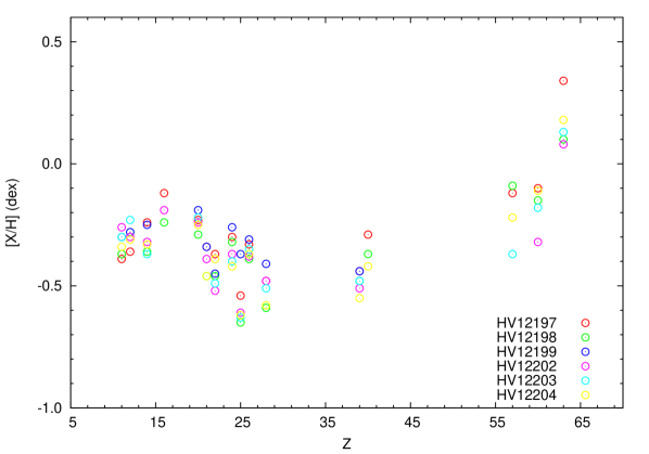
Figure 2: Abundance ratios ([X/H]) for our NGC 1866 Cepheids for different elements identified by their atomic number Z.

With [Fe/H] $\approx$ $-0.4$ dex, our NGC 1866 Cepheids can be compared to Cepheids located in the outer disc of the Milky Way, at Galactocentric distances R_G ¿ 10 kpc. A quick glance at the Cepheid abundances in, e.g., Lemasle et al. (2013), and Genovali et al. (2015) indicates that the [Na/Fe] and [$\alpha$/Fe] abundances in the NGC 1866 Cepheids fall slightly below those observed in the Milky Way Cepheids for the corresponding range of metallicities. The same comparison for neutron-capture elements (in da Silva et al., 2016) is less meaningful as the low S/N of our spectra prevented us from taking the hyperfine structure into account in the current study. The [Y/Fe] ratios appear to be similar, which is not surprising as the hfs corrections reported by da Silva et al. (2016) are small for the Y II lines. The [La/Fe], [Nd/Fe], and [Eu/Fe] ratios appear to be higher than in the Milky Way Cepheids with similar metallicities. This is certainly partially due to the hfs corrections. Indeed da Silva et al. (2016) report that the abundances derived from some of the La II lines can be smaller by up to $\approx$0.2 dex. On the other hand, their hfs corrections for the Eu lines are very small, and they did not apply any correction for Nd, which indicates that at least a fraction of the difference is intrinsic.

Cepheids embedded in open clusters are extremely important: as the clusters’ distances can be determined independently via main sequence or isochrone fitting, their Cepheids can be used to calibrate the period-luminosity relations (e.g., Turner, 2010). Furthermore, they can be used to establish period-age relations since the ages of star clusters can be determined from their resolved color-magnitude diagrams. The search for Cepheids as members of open clusters or OB associations was conducted in a long term effort by, e.g., Turner et al. (2012); Majaess et al. (2013), and references therein as well as by Anderson et al. (2013) and Chen et al. (2015) in recent extensive studies. They combined spatial (position, distance) and kinematic data with additional information (age, [Fe/H]) about the stellar populations of the open clusters and found roughly 30 Cepheids associated with open clusters in the Milky Way. However the maximum number of Cepheids that belong to a given cluster is two, much lower than the 23 Cepheids found in NGC 1866 (e.g., Welch & Stetson, 1993).
Comparing the detailed chemical composition of the Cepheids with the one of the other cluster members, as done for the first time in this paper (see Sect. 4.2), speaks in favor of the Cepheid membership of the cluster and should be considered in the future as an important criterion when seeking to match Cepheids to open clusters. This argument holds only if the photospheric abundances in this evolutionary phase were not altered by stellar evolution. In the case of Cepheids, this is expected only for C, N (the first dredge-up alters the surface composition of C and N, and leaves O unaltered) and probably Na (the Ne–Na cycle brings Na-enriched material to the surface). As far as the Milky Way is concerned, the chemical composition of (RGB) stars in open clusters containing Cepheids is often missing, while the direct measurement of stellar abundances in more distant galaxies is out of reach for the current facilities, with the exception of bright, red supergiants (RSGs, e.g., Davies et al., 2015; Patrick et al., 2015; Gazak et al., 2015). Obtaining detailed abundances from RSGs or cluster integrated light spectroscopy (Colucci et al., 2012a) for those extragalactic clusters harboring Cepheids would allow us to investigate the longstanding issue of a possible metallicity dependence of the period-luminosity relations that might affect the extragalactic distance scale (e.g., Romaniello et al., 2008).

4.2 Comparison with giant stars in NGC 1866 and integrated light spectroscopy

Fig. 3 shows a comparison of the abundance ratios [X/Fe] between the six NGC 1866 Cepheids in our sample and other NGC 1866 stars: the 14 RGB stars of Mucciarelli et al. (2011) for which we show the mean abundance ratios and dispersions and the three stars of Colucci et al. (2012a) displayed individually. We also overplot the cluster mean abundance derived from integrated light spectroscopy by Colucci et al. (2012a). All the abundances have been rescaled to our solar reference values.

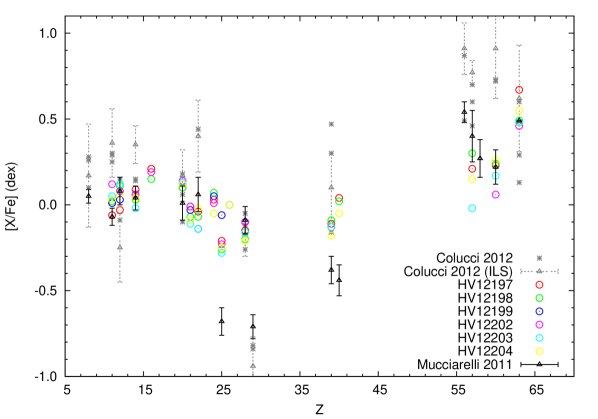
Figure 3: Abundance ratios ([X/Fe]) in NGC 1866 for different elements identified by their atomic number Z. Our Cepheids are the colored open circles, The mean value and dispersion for RGB stars in NGC 1866 from Mucciarelli et al. (2011) are given by the black triangle and solid line. Individual stellar abundances in NGC 1866 by Colucci et al. (2012b) are depicted by gray stars. The mean value and dispersion obtained by Colucci et al. (2012b) via integrated light spectroscopy are indicated by the gray triangle and dotted line. All the abundance ratios have been rescaled to our Solar reference values.

Our Cepheids are slightly enriched in sodium with respect to the RGB stars of Mucciarelli et al. (2011). Similar Na overabundances have already been reported in the Milky Way (e.g., Genovali et al., 2015) when comparing Cepheids and field dwarfs in the thin and thick disc (Soubiran & Girard, 2005). Although this overabundance is probably partially due to NLTE effects (see Sect. 3.6), it has been proposed that it may be caused by mixing events that dredge up material enriched in Na via the NeNa cycle into the surface of the Cepheids (Sasselov, 1986; Denissenkov, 1994; Takeda et al., 2013). Similar Na overabundances have also been observed in RGB stars (e.g., da Silva et al., 2015), reinforcing this hypothesis. It is interesting to note that Na overabundances are quite homogeneous in Cepheids and do not depend on mass or period (Andrievsky et al., 2003; Kovtyukh et al., 2005; Takeda et al., 2013; Genovali et al., 2015). In contrast, da Silva et al. (2015) report a positive trend with mass for [Na/Fe] for RGB stars (which cover a shorter mass range).

The agreement is excellent for the $\alpha$-elements Mg and Si, and to a lesser extent for Ca for which the Cepheid abundances are slightly larger than in the RGB stars. The agreement is good for Fe and excellent for Ni, the only two iron peak elements for which data are available for both RGB stars and Cepheids. For our 6 Cepheids we find a mean [Fe/H] = $-0.36$ dex with a dispersion of 0.03 dex. The 14 RGB stars in Mucciarelli et al. (2011) have an average [Fe/H] of $-0.43$ dex (to which one should add 0.02 dex to take into account differences in the adopted Solar iron abundance) and a dispersion of 0.04 dex.

In contrast, the abundances of some neutron-capture elements are quite discrepant between the two studies: Y and Zr are found significantly more abundant (by 0.25/0.40 dex respectively) than in Mucciarelli et al. (2011). Our abundances of La agree only within the error bars whereas Nd and Eu abundances are in excellent agreement with those reported by these authors. The hfs corrections reported by da Silva et al. (2016) are negligible for Y and therefore cannot account for the difference. In contrast hfs corrections can reach $-0.2$ dex for several La lines, and a good agreement between both studies could be achieved if they were taken into account. A possible explanation for these discrepancies could be that the transitions used to derive the abundances of these elements are associated with different ionization stages. For instance, Allen & Barbuy (2006, their Fig. 13) derived lower Zr abundances from Zr I lines than from Zr II lines in the Barium stars they analyzed, possibly because ionized lines are the dominant species and therefore less affected by departures from the LTE. In the end, their Zr II abundances span a range of 0.40 $\leq$ [Zr II/Fe] $\leq$ 1.60 while their Zr I abundances are found in the $-0.20$ $\leq$ [Zr I/Fe] $\leq$ 1.45 range. Mucciarelli et al. (2011) do not provide their linelist but given the wavelength range of their spectra, it is likely that they used neutral lines. Unfortunately, neutral lines for these elements are too weak and/or blended in the spectra of Cepheids and therefore cannot be measured to test this hypothesis. Only the Zr I lines at 6134.58 and 6143.25 Å, and the Y I line at 6435.05 Å could possibly be measured in the most metal-rich Milky Way Cepheids, but they become too weak already at Solar metallicity.

The abundance ratios derived by Mucciarelli et al. (2011) for NGC 1866 members are in very good agreement with the field RGB stars in the surroundings they analyzed. It is interesting to note that the [La/Fe] and [Eu/Fe] ratios derived in NGC 1866 by Mucciarelli et al. (2011) are in good agreement with other LMC field RGB stars (e.g., Van der Swaelmen et al., 2013, and references therein), while their [Y/Fe] and [Zr/Fe] ratios fall at the lower end of the LMC field stars distribution.

Y and Zr belong to the first peak of the s-process, while La and Ce belong to the second peak of the s-process that is favored when metal-poor AGB stars dominate the chemical enrichment (e.g., Cristallo et al., 2011). The large values of [La/Fe] and [Ce/Fe] demonstrate that the enrichment in heavy elements is dominated by metal-poor AGB stars for both the Cepheids and RGB stars in NGC 1866. Cepheids show higher Y and Zr abundances than RGB stars. If this difference turns out to be real, it might hint that they experienced extra-enrichment in light s-process elements from more metal-rich AGB stars.

Similar conclusions can be drawn when comparing the Cepheid abundances with the stellar abundances derived by Colucci et al. (2012b): the $\alpha$-elements (except Ti) and the iron-peak elements abundance ratios (with respect to iron) they obtained are very similar to those of the Cepheids, while their abundance ratios for the n-capture elements are higher than in the Cepheids, and even higher than those derived by Mucciarelli et al. (2011). Colucci et al. (2012b) did not measure Mn in their NGC 1866 stellar sample. However, they found values ([Mn/Fe]$\approx-0.35$ dex) slightly lower than ours ([Mn/Fe]$\approx-0.25$ dex) in the stars belonging to other young LMC clusters. The Mn abundances reported by Mucciarelli et al. (2011) are also (much) lower than ours. This is almost certainly due to the fact that both studies included hfs corrections for Mn, which are known to be very significant (e.g., Prochaska et al., 2000). Because these ratios are lower than in Milky Way stars of the same metallicity, they proposed that the type Ia supernovae yields of Mn are metallicity-dependent, as reported/modeled in other environments by, e.g., McWilliam et al. (2003), Cescutti et al. (2008), and North et al. (2012).

In contrast, the abundance ratios they derived from integrated light spectroscopy are almost always significantly larger than those obtained for RGB stars by Mucciarelli et al. (2011) or for Cepheids (this study), or at least at the higher end. This might be due to the fact that Colucci et al.’s work based on integrated light includes contributions of many different stellar types (and possibly contaminating field populations). This is nevertheless surprising because the integrated flux originating from a young cluster such as NGC 1866 should be dominated by young supergiants, and one would therefore expect a better match between the Cepheids and the integrated light spectroscopy abundance ratios.

4.3 Multiple stellar populations in NGC 1866

In a recent paper, Milone et al. (2017) reported the discovery of a split main sequence (MS) and of an extended main sequence turn-off in NGC 1866. These intriguing features have already been reported in many of the intermediate-age clusters in the Magellanic Clouds as well as for some of their young clusters (e.g., Bertelli et al., 2003; Glatt et al., 2008; Milone et al., 2013), although there is no agreement whether this is indeed due to multiple stellar populations. The blue MS hosts roughly $\nicefrac{{1}}{{3}}$ of the MS stars, the remaining $\nicefrac{{2}}{{3}}$ belonging to a spatially more concentrated red MS. Milone et al. (2017) rule out the possibility that age variations solely can be responsible for the split of the MS in NGC 1866. Instead, the red MS is consistent with a $\approx$200 Myr old population of extremely fast-rotating stars ($\omega$=0.9$\omega_{c}$) while the blue MS is consistent with non-rotating stars of similar age, including a small fraction of even older stars. However, according to Milone et al. (2017) the upper blue MS can only be reproduced by a somewhat younger population ($\approx$140 Myr old) accounting for roughly 15% of the total MS stars.

As the age range of Cepheids is similar to the one of the NGC 1866 MS stars, it is natural to examine how they fit in the global picture of NGC 1866 drawn by Milone et al. (2017). These authors clearly state in their conclusion that the above interpretation should only be considered as a working hypothesis and our only intent here is to examine if Cepheids can shed some light on this scenario.

It is possible to compute individual ages for Cepheids with a period-age relation derived from pulsation models (e.g., Bono et al., 2005). Because rotation brings fresh material to the core during the MS hydrogen burning phase, fast-rotating stars of intermediate masses stay longer on the MS and therefore cross the instability strip later than a non-rotating star. Including rotation in models then increases the ages of Cepheids by 50 to 100%, depending on the period, as computed by Anderson et al. (2016). Following the prescriptions of Anderson et al. (2016) we derive ages for all the Cepheids known in NGC 1866: we use a period-age relation computed with models with average rotation ($\omega$=0.5$\omega_{c}$) and averaged over the second and third crossing of the instability strip. Periods are taken from Musella et al. (2016). In the absence of further information, we assume that they are fundamental pulsators, except for V5, V6, and V8, as Musella et al. (2016) report that their periods and light curves are typical of first overtone pulsators. Even more importantly they lie on the PL relations of first overtones. For comparison, we also derive ages using the period-age relation from Bono et al. (2005), which was computed using non-rotating pulsation models. Ages are listed in Table 5.

We first notice that in both cases the age spread is very limited, thus reinforcing previous findings stating that there is no age variation within NGC1866, or at least that Cepheids all belong to the same sub-population. As expected, the ages calculated with the period-age relation from Bono et al. (2005) lead to younger Cepheids and therefore appear to be compatible only with the 140 Myr old stars populating the upper part of the blue main sequence. None of the period-age relations by Bono et al. (2005) and Anderson et al. (2016) enables us to compute individual error bars. Uncertainties on the ages of the NGC 1866 Cepheids of the order of 25–30 Myr can be derived by using the standard deviation of the period-age relation by Bono et al. (2005) as the error. However, given quoted error bars of 50% or more (Anderson et al., 2016), an age of 200 Myr cannot be completely excluded. On the other hand, the ages computed with the period-age relation including rotation from Anderson et al. (2016) correspond very well to the fast-rotating red MS population. However the reader should keep in mind that ages should be directly compared only when they are on the same scale, which requires that they were all calculated based on the same models.

Using evolutionary tracks computed with either canonical (no overshooting) or non-canonical (moderate overshooting) assumptions (but no rotation), Musella et al. (2016) favor an age of 140 Myr. The location of the Cepheids, in between the theoretical blue loops computed in each case, does not allow us to discriminate the two overshooting hypotheses. Adopting a canonical overshooting and an older age of 180 Myr enables us to better fit the observed luminosities of the Cepheids, but the theoretical blue loops are then too short to reach the Cepheids’ locus in the CMD. Finally, using high-resolution integrated light spectroscopy and CMD-fitting techniques, Colucci et al. (2011) report a similar age of 130 Myr.

Ages of Cepheids, derived using period-age relations computed with either no rotation or an average rotation ($\omega$=0.5$\omega_{c}$), do not allow us to confirm or rule out the hypothesis of Milone et al. (2017). Unfortunately, Anderson et al. (2016) do not provide period-age relations for fast-rotators ($\omega$=0.9$\omega_{c}$). As far as Cepheid ages are concerned, it is interesting to note that the Cepheids in NGC 1866 match very well the peak of the age distribution for LMC field Cepheids, computed by Inno et al. (2015b) using new period-age relations (without rotation) at LMC metallicities.

Table 5: Individual ages for Cepheids in NGC 1866 computed with the period-age relations of Bono et al. (2005) or Anderson et al. (2016) for fundamental pulsators, and the periods listed in Musella et al. (2016)

Cepheid	Period	Age	Age
		(no rotation)	(rotation: $\omega$=0.5$\omega_{c}$)
	(d)	(Myr)	(Myr)
V6	1.9442620	114.5	258.7
V8	2.0070000	111.7	252.0
V5	2.0390710	110.3	248.7
HV 12199	2.6391600	120.6	222.7
HV 12200	2.7249800	117.6	218.0
We 4	2.8603600	113.2	211.1
WS 5	2.8978000	112.1	209.3
New	2.9429300	110.8	207.1
HV 12203	2.9541100	110.4	206.6
We 8	3.0398490	108.0	202.7
We 3	3.0490400	107.7	202.3
WS 11	3.0533000	107.6	202.1
We 2	3.0548500	107.6	202.1
WS 9	3.0694500	107.2	201.4
V1	3.0845500	106.8	200.8
HV 12202	3.1012000	106.3	200.0
HV 12197	3.1437100	105.2	198.2
We 5	3.1745000	104.4	197.0
We 7	3.2322700	102.9	194.6
We 6	3.2899400	101.5	192.3
V4	3.3180000	100.9	191.3
HV 12204	3.4388200	98.1	186.8
V7	3.4520700	97.8	186.3
HV 12198	3.5228000	96.3	183.8

4.4 The metallicity gradients from Cepheids in the SMC

The existence of a metallicity gradient across the SMC is a long-debated issue. Using large numbers of RGB stars, Carrera et al. (2008); Dobbie et al. (2014), and Parisi et al. (2016) report a radial metallicity gradient ($-0.075\pm 0.011$ dex.deg^-1 vs. $-0.08\pm 0.02$ dex.deg^-1 in the two latter studies) in the inner few degrees of the SMC. In both cases, this effect is attributed to the increasing fraction of younger, more metal-rich stars towards the SMC center. However, the presence of such a gradient was not confirmed by C- and M- type AGB stars (Cioni et al., 2009), populous clusters (e.g., Parisi et al., 2015, 2016, and references therein), or RR Lyrae studies (e.g., Haschke et al., 2012a; Deb et al., 2015; Skowron et al., 2016, and references therein).

The SMC is very elongated and tilted by more than 20^∘ (e.g., Haschke et al., 2012b; Subramanian et al., 2012; Nidever et al., 2013). Moreover, old and young stellar populations have significantly different spatial distributions and orientations (e.g., Haschke et al., 2012b; Jacyszyn-Dobrzeniecka et al., 2017). Recent studies using mid-infrared Spitzer data (Scowcroft et al., 2016) or optical data from the OGLE IV experiment (Jacyszyn-Dobrzeniecka et al., 2016) clearly confirmed this complex shape. Our Cepheid abundances combined with those found in the literature (Romaniello et al., 2008), and the possibility to derive accurate distances thanks to the period-luminosity relations allow us to shed new light on the SMC metallicity distribution. For the first time, we are able to probe the metallicity gradient in the SMC’ young population in the ”depth” direction. As Cepheids are young stars, it should be noted that our study only concerns the present-day abundance gradient, and as such, the metal-rich end of the metallicity distribution function ([Fe/H]$>-0.90$ dex). Moreover, our sample is small (17 stars) and does not contain stars in the inner few degrees of the SMC in an on-sky projection (see Fig. 4). For old populations traced by RR Lyrae stars, no significant metallicity gradient was found in the ”depth” direction (Haschke et al., 2012a).

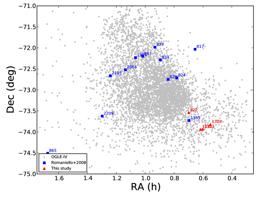
Figure 4: SMC Cepheids with known metallicities (red: this study; blue: Romaniello et al. (2008). SMC Cepheids in the OGLE-IV database are shown as gray dots).

Individual distance moduli for SMC Cepheids were computed using the [3.6] $\mu$m mean-light magnitudes tabulated by Scowcroft et al. (2016) and the corresponding PL-relation in the mid-infrared (MIR) established by the same authors. Combining the extinction law of Indebetouw et al. (2005) with that of Cardelli et al. (1989), Monson et al. (2012) reported a total-to-selective extinction ratio of A_[3.6]/E(B-V)=0.203. We adopted the average color excess found by Scowcroft et al. (2016) for the SMC: E(B-V)=0.071$\pm$0.004 mag, which leads to A_[3.6]=0.014$\pm$0.001 mag. There is no MIR photometry available for HV822 and HV823. For HV822, we use the distance of 67441.4 pc derived by Groenewegen et al. (2013) via the Baade-Wesselink method. The typical uncertainty on the individual MIR distances is of the order of $\pm$3 kpc (Scowcroft et al., 2016).

For comparison purposes, we also computed distances based on NIR photometry. For the Cepheids in the OGLE-IV database, we used near-infrared J, H and K_S magnitudes from the IRSF/SIRIUS catalog (Kato et al., 2007) that were derived by using the near-infrared light-curve templates of Inno et al. (2015a). Distances were computed using period-Wesenheit (PW) relations calibrated on the entire SMC sample of fundamental mode Cepheids ($>$2200 stars Inno et al., 2017, in prep). Wesenheit indices are reddening-free quantities by construction (Madore, 1982). We used the W_HJK index as defined by Inno et al. (2016): W_HJK = $H$–1.046 $\times$ ($J-K_{\rm{S}}$) which is minimally affected by the uncertainty in the reddening law (Inno et al., 2016). For stars that are not in the OGLE-IV database, the same procedure was adopted, except that the distances are derived from 2MASS (Skrutskie et al., 2006) single epoch data (with no template applied). Individual uncertainties on distances are listed in Table 6. The typical uncertainty, computed as the average of the individual uncertainties is 993$\pm$41 pc and can be rounded to 1 kpc. It is beyond the scope of this paper to compare both sets of distances. We simply mention here that they are in very good agreement despite some star-to-star scatter (see Fig. 5).

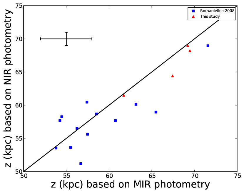
Figure 5: Comparison of distances derived either from near-infrared or from mid-infrared photometry (red: this study; blue: Romaniello et al. (2008). Typical uncertainties are shown in the top left corner.

To investigate the metallicity gradient in the SMC, we combine our [Fe/H] abundances with those of Romaniello et al. (2008), to which we added 0.03 dex to take into account differences in the Solar reference values. The Cepheids were placed in a Cartesian coordinate system using the transformations of van der Marel & Cioni (2001) and Weinberg & Nikolaev (2001). We adopted the value tabulated in SIMBAD for the center of the SMC: $\alpha_{0}$=00h52m38.0s, $\delta_{0}$=-72d48m01.00s (J2000). For the SMC distance modulus, we adopted the value reported by Graczyk et al. (2014) using eclipsing binaries: 18.965$\pm$0.025 (stat.) $\pm$ 0.048 (syst.) mag which translates into a distance of 62.1$\pm$1.9 kpc. Individual distances and abundances can be found in Table 6, as well as ages derived with the period-age relation of Bono et al. (2005).

A first glance at Fig. 6 shows that the (x,y) plane is not very relevant because it does not reflect the depth of the SMC. This fact is reinforced in the case of Cepheids as they are bright stars that can be easily identified and analyzed, even at very large distances. More interesting are the (x,z) and especially the (y,z) plane, as they allow us to study for the first time the metallicity distribution of Cepheids along the SMC main component. Our 17 Cepheids adequately sample the z direction, but the reader should keep in mind that most of our targets are located above the main body of the SMC (see Fig. 4 or Jacyszyn-Dobrzeniecka et al., 2016, their Fig. 16). Fig 6 and Fig 7, where [Fe/H] is plotted as a function of z, show no evidence of a metallicity gradient along the main axis of the SMC. The metallicity spread barely reaches 0.3 dex, but both ends of the z-axis seem to be slightly more metal poor that the inner regions as they miss the more metal-rich Cepheids. The age range spans only 100 Myr and we see no correlation between age and metallicity or distance. These interesting findings should nevertheless be considered only as preliminary results, given the small size of our sample and the location of our Cepheids outside the main body of the SMC.

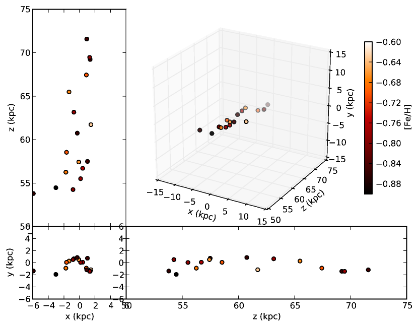
Figure 6: Metallicity distribution of SMC Cepheids in Cartesian coordinates. Distances are based on mid-infrared photometry.

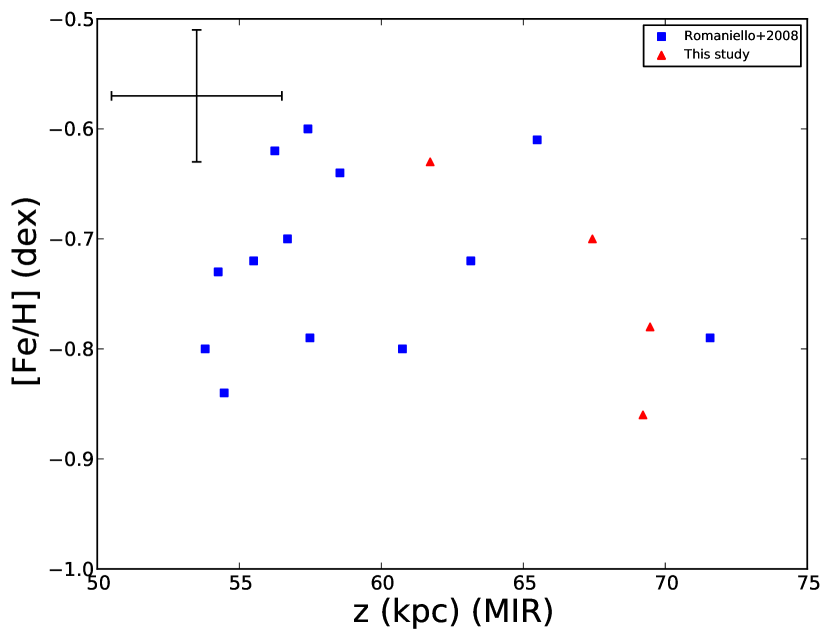
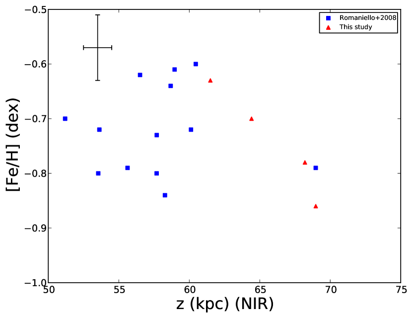
Figure 7: SMC metallicity distribution from Cepheids in the z (depth) direction. Top panel: distances derived from mid-infrared photometry; Bottom panel: distances derived from near-infrared photometry. Typical error bars are shown in the top left corner.

Table 6: Individual distances, ages, and metallicities for SMC Cepheids. Metallicities from Romaniello et al. (2008) have been put on the same metallicity scale (by adding 0.03 dex to them) as our data.

Cepheid	log P	Age	Distance	Distance	Uncertainty on	[Fe/H]
	(d)	(Myr)	(MIR) (pc)	(NIR) (pc)	NIR distances (pc)	(dex)
HV817	1.277	212.4	57502	55636	1136	-0.79
HV823	1.504	186.9	-	60770	964	-0.77
HV824	1.819	161.2	56700	51195	957	-0.70
HV829	1.926	154.2	55506	53625	964	-0.73
HV834	1.867	157.9	57420	60463	1168	-0.60
HV837	1.631	175.5	60752	57692	1033	-0.80
HV847	1.433	194.2	63160	60129	1175	-0.72
HV865	1.523	185.2	54586	58401	1018	-0.84
HV1365	1.094	239.7	71595	68986	1094	-0.79
HV1954	1.222	219.8	54265	57702	1027	-0.73
HV2064	1.527	184.7	65503	58973	1182	-0.61
HV2195	1.621	176.3	58568	58703	1163	-0.64
HV2209	1.355	202.8	56286	56543	1006	-0.62
HV11211	1.330	205.8	54140	53884	966	-0.80
HV822	1.224	219.6	67447	64428	1022	-0.70
HV1328	1.200	223.0	61750	61526	976	-0.63
HV1333	1.212	221.2	69244	69002	1094	-0.86
HV1335	1.158	229.3	69493	68231	1214	-0.78

5 Conclusions

In this paper we conducted a spectroscopic analysis of Cepheids in the LMC and in the SMC. We provide abundances for a good number of $\alpha$, iron-peak, and neutron-capture elements. Our sample increases by 20% (respectively 25%) the number of Cepheids with known metallicities and by 46% (respectively 50%) the number of Cepheids with detailed chemical composition in these galaxies.

For the first time, we study the chemical composition of several Cepheids located in the same populous cluster NGC 1866, in the Large Magellanic Cloud. We find that the six Cepheids we studied have a very homogeneous chemical composition, which is also consistent with RGB stars already analyzed in this cluster. Our results are also in good agreement with theoretical models accounting for luminosity and radial velocity variations for the two stars (HV 12197, HV 12199) for which such measurements are available. Using various versions of period–age relations with no ($\omega$=0) or average rotation ($\omega$=0.5$\omega_{c}$) we find a similar age for all the Cepheids in NGC 1866, indicating that they all belong to the same stellar population.

Using near- or mid-infrared photometry and period-luminosity relations (Inno et al., 2016; Scowcroft et al., 2016), we computed the distances for Cepheids in the SMC. Combining our abundances for Cepheids in the SMC with those of Romaniello et al. (2008), we study for the first time the metallicity distribution of the young population in the SMC in the depth direction. We find no metallicity gradient in the SMC, but our data include only a small number of stars and do not contain Cepheids in the inner few degrees of the SMC.

Appendix A Abundances of the Cepheids in the LMC cluster NGC 1866

Table 7: Chemical composition of HV 12197. For a given element, the abundance (computed as the mean value of the abundances determined for each individual line of this element), rms, and number of lines (N) used is given for each individual spectrum analyzed. The final abundance of a star is computed as the weighted mean (and standard deviation) for the three spectra analyzed, where the weight is the number of lines of a given element measured in each spectrum. We remind the reader that hfs was not taken into account and that the hfs correction might be negligible to severe (up to $-0.2$ dex da Silva et al., 2016) for La and (up to $-0.65$ dex, Lemasle et al., in prep) for Mn, while it is expected to be negligible for Y, Zr, Nd, Eu.

HV 12197	MJD=54806.02457622			MJD=54806.08071473			MJD=54806.13684767			Abundance
Element	[X/H]	$\sigma$	N	[X/H]	$\sigma$	N	[X/H]	$\sigma$	N	[X/H]	$\sigma$
	(dex)	(dex)		(dex)	(dex)		(dex)	(dex)		(dex)	(dex)
[NaI/H]	-0.33		1	-0.37		1	-0.46		1	-0.39	0.04
[MgI/H]	-0.36		1	-0.43		1	-0.29		1	-0.36	0.04
[SiI/H]	-0.16	0.18	3	-0.21	0.19	5	-0.31	0.10	5	-0.24	0.09
[SiII/H]
[SI/H]	-0.06		1	-0.24		1	-0.06		1	-0.12	0.06
[CaI/H]	-0.19	0.06	10	-0.26	0.06	10	-0.23	0.08	11	-0.23	0.04
[ScII/H]	-0.30	0.19	6	-0.34	0.12	6	-0.37	0.16	6	-0.34	0.09
[TiI/H]	-0.55		1	-0.27	0.35	2				-0.36	0.22
[TiII/H]	-0.52		1	-0.36	0.07	2	-0.31	0.16	2	-0.37	0.07
[CrI/H]	-0.24		1							-0.24
[CrII/H]	-0.16	0.11	3	-0.39	0.13	3	-0.35	0.07	4	-0.30	0.06
[MnI/H]				-0.55	0.04	2	-0.52		1	-0.54	0.03
[FeI/H]	-0.31	0.10	27	-0.34	0.11	50	-0.34	0.13	59	-0.33	0.07
[FeII/H]	-0.34	0.16	8	-0.33	0.09	8	-0.33	0.12	9	-0.33	0.07
[NiI/H]	-0.38		1	-0.49	0.17	3	-0.49	0.17	5	-0.48	0.10
[YII/H]	-0.45		1	-0.46	0.06	2	-0.41	0.15	2	-0.44	0.05
[ZrII/H]				-0.31		1	-0.27		1	-0.29	0.02
[LaII/H]				-0.17		1	-0.09	0.16	2	-0.12	0.10
[NdII/H]				-0.09	0.08	3	-0.12	0.06	2	-0.10	0.05
[EuII/H]	0.48		1	0.29		1	0.26		1	0.34	0.07

Table 8: Same as Table 7 for HV 12198.

HV 12198	MJD=54806.02457622			MJD=54806.08071473			MJD=54806.13684767			Abundance
Element	[X/H]	$\sigma$	N	[X/H]	$\sigma$	N	[X/H]	$\sigma$	N	[X/H]	$\sigma$
	(dex)	(dex)		(dex)	(dex)		(dex)	(dex)		(dex)	(dex)
[NaI/H]	-0.37	0.05	2	-0.33		1	-0.40	0.13	2	-0.37	0.05
[MgI/H]	-0.34		1	-0.27		1	-0.23		1	-0.28	0.04
[SiI/H]	-0.34	0.04	2	-0.31	0.28	5	-0.39	0.08	8	-0.36	0.09
[SiII/H]				-0.21		1	-0.27		1	-0.24	0.03
[SI/H]							-0.24		1	-0.24
[CaI/H]	-0.35	0.14	3	-0.26	0.08	4	-0.26	0.05	3	-0.29	0.05
[ScII/H]	-0.50	0.06	2	-0.44	0.21	3	-0.44	0.10	3	-0.46	0.08
[TiI/H]	-0.43		1	-0.48	0.08	3	-0.46	0.15	3	-0.46	0.07
[TiII/H]	-0.31		1	-0.34		1	-0.47		1	-0.37	0.05
[CrI/H]	-0.48		1							-0.48
[CrII/H]	-0.23	0.17	2	-0.35	0.16	3	-0.34	0.09	3	-0.32	0.07
[MnI/H]	-0.64	0.05	2	-0.71	0.04	2	-0.57		1	-0.65	0.03
[FeI/H]	-0.39	0.10	33	-0.37	0.10	50	-0.40	0.07	43	-0.39	0.05
[FeII/H]	-0.41	0.16	4	-0.38	0.11	5	-0.40	0.09	8	-0.40	0.06
[NiI/H]	-0.51	0.16	4	-0.59	0.16	6	-0.62	0.10	8	-0.59	0.07
[YII/H]	-0.38	0.13	2	-0.46	0.15	3	-0.57	0.15	3	-0.48	0.08
[ZrII/H]							-0.37		1	-0.37
[LaII/H]	-0.05	0.01	2	-0.07	0.03	2	-0.16	0.01	2	-0.09	0.02
[NdII/H]	-0.16	0.09	2	-0.15	0.05	3	-0.15	0.08	3	-0.15	0.04
[EuII/H]	0.10		1	0.12		1	0.09	0.16	2	0.10	0.07

Table 9: Same as Table 7 for HV 12199.

HV 12199	MJD=54806.02457622			MJD=54806.08071473			MJD=54806.13684767			Abundance
Element	[X/H]	$\sigma$	N	[X/H]	$\sigma$	N	[X/H]	$\sigma$	N	[X/H]	$\sigma$
	(dex)	(dex)		(dex)	(dex)		(dex)	(dex)		(dex)	(dex)
[NaI/H]	-0.33		1	-0.27	0.03	2	-0.31	0.01	2	-0.30	0.02
[MgI/H]	-0.26		1	-0.31		1	-0.27		1	-0.28	0.01
[SiI/H]	-0.23	0.11	2	-0.31	0.05	3	-0.20	0.09	3	-0.25	0.04
[SiII/H]
[SI/H]
[CaI/H]	-0.17	0.12	10	-0.22	0.06	11	-0.17	0.11	11	-0.19	0.05
[ScII/H]	-0.32	0.21	3	-0.35	0.10	5	-0.34	0.11	6	-0.34	0.07
[TiI/H]				-0.47		1				-0.47
[TiII/H]	-0.44	0.05	3	-0.48	0.03	2	-0.40		1	-0.45	0.03
[CrI/H]	-0.25		1				-0.36		1	-0.30	0.05
[CrII/H]	-0.29	0.26	3	-0.16	0.08	2	-0.29	0.18	4	-0.26	0.11
[MnI/H]							-0.37	0.18	2	-0.37	0.18
[FeI/H]	-0.29	0.10	29	-0.30	0.05	35	-0.32	0.10	49	-0.31	0.05
[FeII/H]	-0.30	0.09	8	-0.30	0.11	9	-0.31	0.15	11	-0.30	0.07
[NiI/H]	-0.33	0.15	3	-0.42		1	-0.53	0.06	2	-0.41	0.08
[YII/H]	-0.32		1	-0.48		1	-0.48	0.08	2	-0.44	0.05
[ZrII/H]
[LaII/H]
[NdII/H]
[EuII/H]

Table 10: Same as Table 7 for HV 12202.

HV 12202	MJD=54806.02457622			MJD=54806.08071473			MJD=54806.13684767			Abundance
Element	[X/H]	$\sigma$	N	[X/H]	$\sigma$	N	[X/H]	$\sigma$	N	[X/H]	$\sigma$
	(dex)	(dex)		(dex)	(dex)		(dex)	(dex)		(dex)	(dex)
[NaI/H]	-0.31		1	-0.26		1	-0.23	0.06	2	-0.26	0.03
[MgI/H]	-0.28		1	-0.32		1	-0.30		1	-0.30	0.01
[SiI/H]	-0.31	0.18	3	-0.31	0.14	4	-0.33	0.03	3	-0.32	0.07
[SiII/H]				-0.17		1				-0.17
[SI/H]				-0.09		1	-0.29		1	-0.19	0.10
[CaI/H]	-0.35	0.13	9	-0.21	0.10	9	-0.17	0.08	9	-0.24	0.06
[ScII/H]	-0.45	0.23	3	-0.39	0.20	3	-0.30	0.03	2	-0.39	0.10
[TiI/H]	-0.68		1	-0.48		1	-0.40		1	-0.52	0.08
[TiII/H]				-0.40		1				-0.40
[CrI/H]
[CrII/H]	-0.32	0.14	4	-0.40	0.19	3	-0.40	0.14	3	-0.37	0.08
[MnI/H]	-0.71	0.02	1	-0.58	0.03	3				-0.61	0.04
[FeI/H]	-0.38	0.08	29	-0.41	0.07	44	-0.36	0.10	41	-0.38	0.05
[FeII/H]	-0.39	0.05	6	-0.40	0.15	5	-0.38	0.14	6	-0.39	0.06
[NiI/H]	-0.54	0.03	3	-0.53	0.08	2	-0.41	0.12	4	-0.48	0.06
[YII/H]	-0.40	0.01		-0.54		1	-0.58		1	-0.51	0.05
[ZrII/H]
[LaII/H]
[NdII/H]	-0.25		1				-0.39		1	-0.32	0.07
[EuII/H]				0.08		1				0.08

Table 11: Same as Table 7 for HV 12203.

HV 12203	MJD=54806.02457622			MJD=54806.08071473			MJD=54806.13684767			Abundance
Element	[X/H]	$\sigma$	N	[X/H]	$\sigma$	N	[X/H]	$\sigma$	N	[X/H]	$\sigma$
	(dex)	(dex)		(dex)	(dex)		(dex)	(dex)		(dex)	(dex)
[NaI/H]				-0.30		1				-0.30
[MgI/H]	-0.18		1	-0.18		1	-0.34		1	-0.23	0.05
[SiI/H]	-0.28	0.12	3	-0.38	0.05	3	-0.41	0.10	5	-0.37	0.05
[SiII/H]							-0.23		1	-0.23
[SI/H]
[CaI/H]	-0.25	0.13	4	-0.18	0.10	9	-0.25	0.12	6	-0.22	0.06
[ScII/H]	-0.33	0.22	5	-0.55	0.20	3	-0.57	0.02	3	-0.46	0.11
[TiI/H]				-0.46		1	-0.53		1	-0.49	0.04
[TiII/H]
[CrI/H]
[CrII/H]	-0.25	0.33	2	-0.46	0.13	4	-0.42	0.22	3	-0.40	0.11
[MnI/H]	-0.71		1	-0.59	0.11	2	-0.64	0.06	2	-0.63	0.05
[FeI/H]	-0.33	0.14	32	-0.36	0.08	37	-0.36	0.12	45	-0.35	0.07
[FeII/H]	-0.36	0.06	5	-0.39	0.11	2	-0.35	0.16	8	-0.36	0.09
[NiI/H]	-0.51	0.20	5	-0.45	0.06	3	-0.56	0.20	4	-0.51	0.10
[YII/H]	-0.34	0.19	2	-0.62	0.11	2	-0.49	0.11	2	-0.48	0.08
[ZrII/H]
[LaII/H]				-0.37	0.01	2				-0.37	0.01
[NdII/H]				-0.24	0.16	2	-0.12	0.13	2	-0.18	0.09
[EuII/H]				0.13	0.06	2				0.13	0.06

Table 12: Same as Table 7 for HV 12204.

HV 12204	MJD=54806.02457622			MJD=54806.08071473			MJD=54806.13684767			Abundance
Element	[X/H]	$\sigma$	N	[X/H]	$\sigma$	N	[X/H]	$\sigma$	N	[X/H]	$\sigma$
	(dex)	(dex)		(dex)	(dex)		(dex)	(dex)		(dex)	(dex)
[NaI/H]	-0.37	0.08	2	-0.32	0.05	2	-0.34		1	-0.34	0.03
[MgI/H]	-0.34		1	-0.26		1	-0.32		1	-0.31	0.02
[SiI/H]	-0.34	0.08	6	-0.36	0.02	6	-0.30	0.12	6	-0.33	0.05
[SiII/H]	-0.21		1	-0.18		1	-0.22		1	-0.20	0.01
[SI/H]
[CaI/H]	-0.28	0.05	9	-0.21	0.07	10	-0.26	0.05	6	-0.25	0.03
[ScII/H]	-0.47	0.19	5	-0.47	0.15	6	-0.44	0.08	4	-0.46	0.08
[TiI/H]	-0.46	0.13	2	-0.42	0.11	3	-0.33	0.27	4	-0.39	0.12
[TiII/H]	-0.64		1	-0.45	0.08	3	-0.43	0.06	3	-0.47	0.05
[CrI/H]				-0.56		1	-0.53		1	-0.55	0.02
[CrII/H]	-0.47	0.06	2	-0.38	0.13	4	-0.46	0.28	2	-0.42	0.08
[MnI/H]	-0.64		1	-0.61		1	-0.60		1	-0.62	0.01
[FeI/H]	-0.38	0.07	44	-0.34	0.10	56	-0.38	0.10	57	-0.37	0.05
[FeII/H]	-0.38	0.14	9	-0.35	0.09	10	-0.39	0.10	11	-0.37	0.06
[NiI/H]	-0.51	0.10	5	-0.60	0.10	7	-0.60	0.14	7	-0.58	0.07
[YII/H]	-0.54	0.02	3	-0.43	0.11	2	-0.62	0.09	4	-0.55	0.05
[ZrII/H]				-0.42		1	-0.43		1	-0.42	0.01
[LaII/H]	-0.17		1	-0.25	0.18	3	-0.21	0.15	5	-0.22	0.10
[NdII/H]	-0.06	0.26	2	-0.11	0.04	3	-0.15	0.02	3	-0.11	0.06
[EuII/H]				0.18		1				0.18

Appendix B Abundances of the Cepheids in the SMC field

Table 13: Same as Table 7 for HV 822.

HV 822	MJD=54785.04026326			MJD=54785.05240828			MJD=54785.06455378			Abundance
Element	[X/H]	$\sigma$	N	[X/H]	$\sigma$	N	[X/H]	$\sigma$	N	[X/H]	$\sigma$
	(dex)	(dex)		(dex)	(dex)		(dex)	(dex)		(dex)	(dex)
[NaI/H]				-0.90		1	-0.83		1	-0.86	0.04
[MgI/H]				-0.79		1	-0.75		1	-0.77	0.02
[SiI/H]	-0.62	0.04	2	-0.67	0.13	3	-0.75	0.03	2	-0.68	0.05
[SiII/H]
[SI/H]				-0.54		1				-0.54
[CaI/H]	-0.52	0.15	9	-0.58	0.14	10	-0.59	0.13	9	-0.56	0.08
[ScII/H]	-0.96	0.18	6	-0.96	0.15	6	-1.00	0.18	5	-0.97	0.09
[TiI/H]
[TiII/H]	-0.80	0.21	4	-0.78	0.24	3	-0.80	0.21	3	-0.79	0.11
[CrI/H]				-0.66		1				-0.66
[CrII/H]	-0.76	0.16	4	-0.77	0.13	4	-0.77	0.21	3	-0.77	0.09
[MnI/H]
[FeI/H]	-0.66	0.08	35	-0.71	0.06	31	-0.63	0.13	38	-0.66	0.06
[FeII/H]	-0.72	0.12	12	-0.77	0.11	11	-0.74	0.09	11	-0.74	0.06
[NiI/H]	-0.82		1	-0.87		1				-0.84	0.03
[YII/H]	-1.18		1	-1.00	0.27	2				-1.06	0.17
[ZrII/H]							-0.73		1	-0.73
[LaII/H]
[NdII/H]
[EuII/H]

Table 14: Same as Table 7 for HV 1328.

HV 1328	MJD=54785.00779033			MJD=54785.01762254			MJD=54785.02744873			Abundance
Element	[X/H]	$\sigma$	N	[X/H]	$\sigma$	N	[X/H]	$\sigma$	N	[X/H]	$\sigma$
	(dex)	(dex)		(dex)	(dex)		(dex)	(dex)		(dex)	(dex)
[NaI/H]	-0.79		1	-0.80		1	-0.79		1	-0.79	0.01
[MgI/H]	-0.70		1	-0.69		1	-0.71		1	-0.70	0.01
[SiI/H]	-0.59	0.09	4	-0.68	0.14	2	-0.60	0.17	4	-0.61	0.07
[SiII/H]	-0.32		1							-0.32
[SI/H]	-0.55		1	-0.55		1				-0.55
[CaI/H]	-0.58	0.07	10	-0.61	0.06	10	-0.64	0.05	10	-0.61	0.04
[ScII/H]	-0.66	0.17	5	-0.68	0.14	6	-0.71	0.16	4	-0.68	0.08
[TiI/H]	-0.76		1	-0.79		1	-0.83		1	-0.79	0.02
[TiII/H]	-0.74	0.05	4	-0.67	0.08	4	-0.67	0.13	5	-0.69	0.06
[CrI/H]							-0.69	0.08	2	-0.69	0.08
[CrII/H]	-0.54	0.11	2	-0.62	0.15	4	-0.63	0.15	4	-0.61	0.08
[MnI/H]	-0.85		1	-0.92		1				-0.89	0.04
[FeI/H]	-0.65	0.05	43	-0.66	0.08	47	-0.66	0.09	54	-0.66	0.05
[FeII/H]	-0.62	0.07	11	-0.59	0.09	10	-0.60	0.10	12	-0.60	0.05
[NiI/H]	-1.00	0.06	2	-1.02	0.11	2	-1.01	0.05	2	-1.01	0.03
[YII/H]	-0.89	0.16	2	-0.87	0.14	2	-0.94	0.11	2	-0.90	0.06
[ZrII/H]	-0.66		1	-0.66		1	-0.70		1	-0.67	0.01
[LaII/H]	-0.21		1				-0.38	0.18	2	-0.32	0.12
[NdII/H]	-0.50		1	-0.47		1	-0.49	0.04	2	-0.49	0.02
[EuII/H]	-0.04		1				-0.08		1	-0.06	0.02

Table 15: Same as Table 7 for HV 1333.

HV 1333	MJD=54785.07912217			MJD=54785.09358357			MJD=54785.10804394			Abundance
Element	[X/H]	$\sigma$	N	[X/H]	$\sigma$	N	[X/H]	$\sigma$	N	[X/H]	$\sigma$
	(dex)	(dex)		(dex)	(dex)		(dex)	(dex)		(dex)	(dex)
[NaI/H]	-0.95		1	-0.97		1				-0.96	0.01
[MgI/H]	-0.89		1	-0.67		1	-0.82		1	-0.79	0.06
[SiI/H]	-0.88	0.10	4	-0.68	0.13	3				-0.79	0.08
[SiII/H]
[SI/H]
[CaI/H]	-0.81	0.09	8	-0.69	0.10	8	-0.82	0.12	8	-0.77	0.06
[ScII/H]	-0.96	0.10	2	-0.92	0.10	2	-0.81		1	-0.91	0.05
[TiI/H]	-1.00	0.08	2	-0.91		1	-0.97	0.06	2	-0.97	0.04
[TiII/H]	-0.94	0.13	3	-0.83	0.20	3	-0.92	0.15	5	-0.90	0.09
[CrI/H]
[CrII/H]	-0.89	0.13	3	-0.92	0.16	4	-0.89	0.08	4	-0.90	0.07
[MnI/H]	-1.19	0.02	2	-1.15		1	-1.20		1	-1.18	0.02
[FeI/H]	-0.90	0.08	40	-0.80	0.05	34	-0.88	0.08	41	-0.86	0.04
[FeII/H]	-0.88	0.10	10	-0.80	0.10	8	-0.89	0.12	7	-0.86	0.06
[NiI/H]	-1.09	0.15	4	-1.06	0.14	5	-1.09	0.15	4	-1.08	0.08
[YII/H]	-1.10	0.07	5	-1.01	0.08	4	-1.10	0.09	3	-1.07	0.04
[ZrII/H]	-0.76		1	-0.57		1	-0.71		1	-0.68	0.06
[LaII/H]	-0.78	0.24	3	-0.52	0.17	3	-0.54	0.08	3	-0.61	0.10
[NdII/H]	-0.50	0.13	3	-0.50	0.16	4	-0.49	0.10	3	-0.50	0.07
[EuII/H]	-0.36		1	-0.33		1				-0.34	0.01

Table 16: Same as Table 7 for HV 1335.

HV 1335	MJD=54785.12765152			MJD=54785.14326987			MJD=54785.15889887			Abundance
Element	[X/H]	$\sigma$	N	[X/H]	$\sigma$	N	[X/H]	$\sigma$	N	[X/H]	$\sigma$
	(dex)	(dex)		(dex)	(dex)		(dex)	(dex)		(dex)	(dex)
[NaI/H]	-0.99		1	-1.02		1	-0.87		1	-0.96	0.04
[MgI/H]	-0.90		1	-0.78		1	-0.81		1	-0.83	0.04
[SiI/H]	-0.92		1	-0.73		2				-0.79	0.06
[SiII/H]	-0.88		1	-1.02		1	-0.78		1	-0.89	0.07
[SI/H]	-0.71		1							-0.71
[CaI/H]	-0.77	0.06	9	-0.71	0.10	10	-0.75	0.06	9	-0.74	0.04
[ScII/H]	-0.93	0.16	5	-0.80	0.17	7	-0.92	0.20	7	-0.88	0.10
[TiI/H]	-0.91	0.21	2	-0.81		1	-1.05		1	-0.92	0.10
[TiII/H]	-0.90	0.13	4	-0.87	0.11	5	-0.90	0.09	6	-0.89	0.06
[CrI/H]	-0.78		1	-0.65		1				-0.72	0.07
[CrII/H]	-0.85	0.22	3	-0.83	0.10	4	-0.87	0.16	3	-0.85	0.08
[MnI/H]	-1.06	0.03	2	-1.08	0.02	2	-1.17		1	-1.09	0.03
[FeI/H]	-0.80	0.08	48	-0.72	0.06	47	-0.82	0.06	46	-0.78	0.04
[FeII/H]	-0.80	0.07	13	-0.73	0.09	14	-0.80	0.09	14	-0.78	0.05
[NiI/H]	-1.01	0.03	3	-0.97	0.10	4	-1.01	0.09	2	-0.99	0.05
[YII/H]	-1.00	0.10	4	-0.93	0.09	3	-1.02	0.18	4	-0.99	0.07
[ZrII/H]	-0.64		1	-0.58		1	-0.72		1	-0.65	0.04
[LaII/H]	-0.58	0.13	4	-0.57	0.11	4	-0.67	0.12	4	-0.61	0.07
[NdII/H]	-0.51	0.05	3	-0.49	0.04	3	-0.49	0.06	3	-0.50	0.03
[EuII/H]	-0.23	0.08	2	-0.15		1				-0.20	0.05

Appendix C List of lines measured

Wavelength	Element	chiex	$log\leavevmode\nobreak\ gf$	Wavelength	Element	chiex	$log\leavevmode\nobreak\ gf$
(Å)		( )	()	(Å)		( )	()
4874.010	Ti2	3.09	-0.809	5627.497	Fe2	3.39	-4.10
4892.859	Fe1	4.22	-1.292	5633.946	Fe1	4.99	-0.23
4893.820	Fe2	2.83	-4.273	5638.262	Fe1	4.22	-0.77
4917.230	Fe1	4.19	-1.089	5641.000	Sc2	1.50	-1.13
4950.106	Fe1	3.42	-1.672	5641.434	Fe1	4.26	-1.08
4959.115	Nd2	0.06	-0.806	5645.613	Si1	4.93	-2.04
5005.157	Ti2	1.57	-2.737	5657.896	Sc2	1.51	-0.60
5017.570	Ni1	3.54	-0.024	5658.816	Fe1	3.40	-0.81
5044.211	Fe1	2.85	-2.045	5665.555	Si1	4.92	-1.94
5084.089	Ni1	3.68	-0.088	5667.149	Sc2	1.50	-1.31
5092.788	Nd2	0.38	-0.618	5669.042	Sc2	1.50	-1.20
5112.270	Zr2	1.66	-0.856	5679.023	Fe1	4.65	-0.82
5114.560	La2	0.23	-1.033	5682.633	Na1	2.10	-0.71
5119.112	Y2	0.99	-1.369	5684.202	Sc2	1.51	-1.07
5129.152	Ti2	1.89	-1.249	5686.530	Fe1	4.55	-0.66
5130.586	Nd2	1.30	0.450	5688.205	Na1	2.10	-0.40
5133.688	Fe1	4.18	0.148	5690.430	Si1	4.93	-1.77
5153.402	Na1	2.10	-1.740	5693.620	Fe1	4.96	-2.59
5155.125	Ni1	3.90	-0.560	5701.544	Fe1	2.56	-2.16
5155.762	Ni1	3.90	0.070	5705.464	Fe1	4.30	-1.35
5159.058	Fe1	4.28	-0.828	5708.400	Si1	4.95	-1.37
5176.559	Ni1	3.90	-0.300	5711.088	Mg1	4.34	-1.83
5196.059	Fe1	4.26	-0.496	5717.833	Fe1	4.28	-1.03
5210.385	Ti1	0.05	-0.835	5731.762	Fe1	4.26	-1.20
5216.274	Fe1	1.61	-2.081	5732.860	Fe1	4.10	-2.90
5217.389	Fe1	3.21	-1.121	5737.059	V1	1.06	-0.74
5305.853	Cr2	3.83	-2.363	5740.858	Nd2	1.16	-0.53
5307.361	Fe1	1.61	-2.911	5741.860	Fe1	4.26	-1.67
5329.138	Cr1	2.91	-0.061	5752.032	Fe1	4.55	-1.18
5329.990	Fe1	4.08	-1.198	5753.120	Fe1	4.26	-0.69
5334.869	Cr2	4.07	-1.617	5853.668	Ba2	0.60	-0.91
5336.771	Ti2	1.58	-1.638	5859.586	Fe1	4.55	-0.42
5345.796	Cr1	1.00	-0.950	5862.357	Fe1	4.55	-0.13
5349.465	Ca1	2.71	-0.311	5866.451	Ti1	1.07	-0.78
5353.370	Fe1	4.10	-0.840	5899.300	Ti1	1.05	-1.17
5369.961	Fe1	4.37	0.537	5905.671	Fe1	4.65	-0.69
5373.709	Fe1	4.47	-0.767	5909.973	Fe1	3.21	-2.59
5379.574	Fe1	3.69	-1.519	5916.247	Fe1	2.45	-2.91
5381.015	Ti2	1.57	-1.977	5927.789	Fe1	4.65	-0.99
5383.369	Fe1	4.31	0.641	5930.179	Fe1	4.65	-0.23
5398.279	Fe1	4.44	-0.634	5934.655	Fe1	3.93	-1.07
5402.774	Y2	1.84	-0.634	5948.541	Si1	5.08	-1.13
5410.910	Fe1	4.47	0.407	5956.694	Fe1	0.86	-4.55
5414.073	Fe2	3.22	-3.582	5976.777	Fe1	3.94	-1.24
5420.922	Cr2	3.76	-2.466	5983.680	Fe1	4.55	-1.47
5425.254	Fe1	1.01	-2.121	5984.815	Fe1	4.73	-0.20
5445.042	Fe1	4.39	-0.029	5987.065	Fe1	4.80	-0.43
5454.090	Ti2	1.57	-3.547	5991.376	Fe2	3.15	-3.65
5462.960	Fe1	4.47	-0.047	6003.011	Fe1	3.88	-1.12
5463.276	Fe1	4.43	0.073	6007.960	Fe1	4.65	-0.60
5501.465	Fe1	0.96	-3.056	6008.556	Fe1	3.88	-0.99
5502.067	Cr2	4.17	-2.097	6013.513	Mn1	3.07	-0.35
5509.895	Y2	0.99	-0.959	6016.673	Mn1	3.07	-0.18
5526.790	Sc2	1.77	0.027	6020.169	Fe1	4.61	-0.27
5528.405	Mg1	4.35	-0.625	6021.819	Mn1	3.08	-0.05
5572.842	Fe1	3.40	-0.270	6024.058	Fe1	4.55	-0.12
5576.089	Fe1	3.43	-0.903	6027.051	Fe1	4.08	-1.09
5581.965	Ca1	2.52	-0.552	6055.990	Fe1	4.73	-0.46
5590.114	Ca1	2.52	-0.572	6065.482	Fe1	2.61	-1.47
5591.370	Fe2	3.27	-4.597	6078.491	Fe1	4.80	-0.32
5601.277	Ca1	2.53	-0.523	6079.008	Fe1	4.65	-1.02

Wavelength	Element	chiex	$log\leavevmode\nobreak\ gf$	Wavelength	Element	chiex	$log\leavevmode\nobreak\ gf$
(Å)		( )	()	(Å)		( )	()
6082.710	Fe1	2.22	-3.57	6335.330	Fe1	2.20	-2.18
6084.111	Fe2	3.20	-3.88	6336.823	Fe1	3.69	-0.86
6085.270	Fe1	2.76	-2.86	6344.148	Fe1	2.43	-2.90
6091.919	Si1	5.87	-1.47	6347.109	Si2	8.12	0.17
6096.664	Fe1	3.98	-1.83	6355.028	Fe1	2.85	-2.32
6102.180	Fe1	4.84	-0.10	6358.697	Fe1	0.86	-4.47
6102.723	Ca1	1.88	-0.79	6362.338	Zn1	5.80	0.14
6108.107	Ni1	1.68	-2.44	6369.462	Fe2	2.89	-4.11
6113.322	Fe2	3.22	-4.23	6380.743	Fe1	4.19	-1.37
6122.217	Ca1	1.89	-0.32	6390.477	La2	0.32	-1.41
6127.906	Fe1	4.14	-1.40	6393.600	Fe1	2.43	-1.50
6141.713	Ba2	0.70	-0.03	6407.251	Fe2	3.89	-3.85
6149.258	Fe2	3.89	-2.84	6408.018	Fe1	3.69	-1.02
6151.617	Fe1	2.18	-3.31	6411.648	Fe1	3.65	-0.66
6155.134	Si1	5.62	-0.75	6414.980	Si1	5.87	-1.04
6157.728	Fe1	4.08	-1.16	6416.919	Fe2	3.89	-2.88
6160.747	Na1	2.10	-1.25	6419.980	Fe1	4.73	-0.17
6161.297	Ca1	2.52	-1.27	6421.350	Fe1	2.28	-2.02
6162.173	Ca1	1.90	-0.09	6430.845	Fe1	2.18	-1.98
6165.360	Fe1	4.14	-1.47	6432.680	Fe2	2.89	-3.57
6166.439	Ca1	2.52	-1.14	6433.457	Si1	5.96	-2.06
6169.042	Ca1	2.52	-0.80	6437.640	Eu2	1.32	-0.32
6169.563	Ca1	2.53	-0.48	6439.075	Ca1	2.52	0.39
6170.506	Fe1	4.79	-0.44	6449.808	Ca1	2.52	-0.50
6173.334	Fe1	2.22	-2.88	6455.598	Ca1	2.52	-1.29
6175.360	Ni1	4.09	-0.39	6462.567	Ca1	2.52	0.26
6176.807	Ni1	4.09	-0.26	6471.662	Ca1	2.53	-0.69
6180.203	Fe1	2.73	-2.62	6481.870	Fe1	2.28	-2.99
6187.989	Fe1	3.94	-1.62	6482.796	Ni1	1.93	-2.63
6191.558	Fe1	2.43	-1.42	6491.561	Ti2	2.06	-1.94
6200.313	Fe1	2.61	-2.40	6493.781	Ca1	2.52	-0.11
6213.430	Fe1	2.22	-2.48	6494.980	Fe1	2.40	-1.26
6215.150	Fe1	4.19	-1.14	6496.897	Ba2	0.60	-0.41
6216.354	V1	0.28	-1.29	6498.938	Fe1	0.96	-4.69
6219.281	Fe1	2.20	-2.43	6499.650	Ca1	2.52	-0.82
6229.226	Fe1	2.85	-2.80	6516.080	Fe2	2.89	-3.31
6230.722	Fe1	2.56	-1.28	6518.366	Fe1	2.83	-2.37
6232.640	Fe1	3.65	-1.22	6559.588	Ti2	2.05	-2.17
6237.319	Si1	5.61	-0.98	6569.214	Fe1	4.73	-0.38
6238.392	Fe2	3.89	-2.60	6572.779	Ca1	0.00	-4.24
6239.370	Fe2	2.81	-4.76	6586.308	Ni1	1.95	-2.75
6239.953	Fe2	3.89	-3.57	6592.913	Fe1	2.73	-1.47
6240.646	Fe1	2.22	-3.20	6593.870	Fe1	2.43	-2.39
6243.815	Si1	5.62	-1.24	6604.601	Sc2	1.36	-1.31
6244.466	Si1	5.62	-1.09	6606.949	Ti2	2.06	-2.80
6245.637	Sc2	1.51	-1.02	6609.110	Fe1	2.56	-2.68
6246.318	Fe1	3.60	-0.80	6613.733	Y2	1.75	-0.85
6247.557	Fe2	3.89	-2.43	6645.064	Eu2	1.38	0.12
6252.555	Fe1	2.40	-1.72	6677.990	Fe1	2.69	-1.37
6254.258	Fe1	2.28	-2.43	6680.133	Ti2	3.09	-1.79
6258.100	Ti1	1.44	-0.30	6680.140	Cr1	4.16	-0.39
6261.100	Ti1	1.43	-0.42	6703.566	Fe1	2.76	-3.06
6262.290	La2	0.40	-1.22	6715.410	Fe1	4.61	-1.36
6265.132	Fe1	2.18	-2.54	6717.681	Ca1	2.71	-0.52
6271.278	Fe1	3.33	-2.70	6721.848	Si1	5.86	-1.52
6279.753	Sc2	1.50	-1.25	6726.666	Fe1	4.61	-1.13
6290.965	Fe1	4.73	-0.77	6740.080	Nd2	0.06	-1.53
6297.793	Fe1	2.22	-2.70	6748.837	S1	7.87	-0.64
6301.500	Fe1	3.65	-0.72	6750.152	Fe1	2.42	-2.60
6318.018	Fe1	2.45	-1.80	6757.171	S1	7.87	-0.24
6318.717	Mg1	5.11	-2.10	6767.768	Ni1	1.83	-2.17
6320.410	La2	0.17	-1.33	6772.313	Ni1	3.66	-0.80
6320.851	Sc2	1.50	-1.82	6774.270	La2	0.13	-1.71
6322.685	Fe1	2.59	-2.45	6795.414	Y2	1.74	-1.03
6327.593	Ni1	1.68	-3.15

Appendix D Curves of growth

The curve of growth is a graph showing how the equivalent width (EW) of an absorption line varies with the abundance (A) of the atoms/ions producing the line. When there are few atoms, the line profile is dominated by Doppler broadening and EW $\propto$ A. When the line reaches saturation, EW $\propto$ $\sqrt{ln\leavevmode\nobreak\ A}$. When saturation increases, the line profile becomes dominated by the wings due to collisional broadening and EW $\propto$ $\sqrt{A}$.

For weak lines it can be shown that $\log\left(\frac{W_{\lambda}}{\lambda}\right)$ varies linearly with $\log(\alpha_{*}gf)$. The $\Gamma_{*}$ quantity, defined as $\log\left(\frac{W_{\lambda}}{\lambda}\right)=\log(\alpha_{*}gf)+\log\Gamma_{*}$ can be computed for each individual line as a function of the atmosphere model, the element considered and its ionization stage, the line excitation potential etc. As the value of the stellar abundance $\alpha_{*}$ is the unknown one wants to determine, the abundance of the same element in the Sun $\alpha_{\odot}$ is used instead. The experimental curves of growth will then be shifted from the theoretical curves of growth by a factor $log(\alpha_{*})-log(\alpha_{\odot})$, which is by definition the abundance ratio [X/H] of the considered element X.

The experimental curve of growth is traced using many lines from the same element (e.g., Fe I) with a wide range of excitation potentials and oscillator strengths that lead to a wide range of equivalent widths. The curves of growth plotted below show the theoretical curves of growths computed for a line at $\lambda$=5000 Å with $\chi_{ex}$ = 3 and using the atmospheric parameters derived for the star in the corresponding phase.

Figure 8: Curves of growth (Fe I, Fe II) for the HV 12197 spectra. From left to right, MJD=54806.02457622, 54806.08071473, MJD=54806.13684767

(a)

(b)

(c)

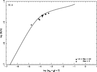
(d)

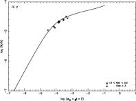
(e)

(f)

Figure 9: Curves of growth (Fe I, Fe II) for the HV 12198 spectra. From left to right, MJD=54806.02457622, 54806.08071473, MJD=54806.13684767

(a)

(b)

(c)

(d)

(e)

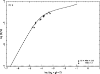
(f)

Figure 10: Curves of growth (Fe I, Fe II) for the HV 12199 spectra. From left to right, MJD=54806.02457622, 54806.08071473, MJD=54806.13684767

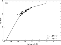
(a)

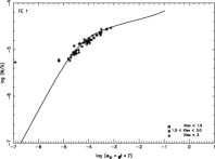
(b)

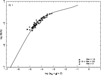
(c)

(d)

(e)

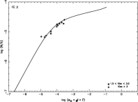
(f)

Figure 11: Curves of growth (Fe I, Fe II) for the HV 12202 spectra. From left to right, MJD=54806.02457622, 54806.08071473, MJD=54806.13684767

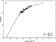
(a)

(b)

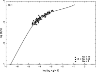
(c)

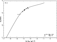
(d)

(e)

(f)

Figure 12: Curves of growth (Fe I, Fe II) for the HV 12203 spectra. From left to right, MJD=54806.02457622, 54806.08071473, MJD=54806.13684767

(a)

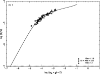
(b)

(c)

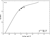
(d)

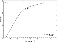
(e)

(f)

Figure 13: Curves of growth (Fe I, Fe II) for the HV 12204 spectra. From left to right, MJD=54806.02457622, 54806.08071473, MJD=54806.13684767

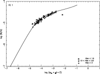
(a)

(b)

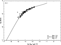
(c)

(d)

(e)

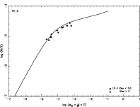
(f)

Figure 14: Curves of growth (Fe I, Fe II) for the HV 822 spectra. From left to right, MJD=54785.04026326, 54785.05240828, 54785.06455378

(a)

(b)

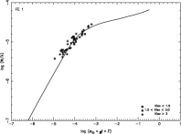
(c)

(d)

(e)

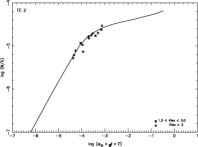
(f)

Figure 15: Curves of growth (Fe I, Fe II) for the HV 1328 spectra. From left to right, MJD=54785.00779033, 54785.01762254, 54785.02744873

(a)

(b)

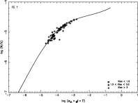
(c)

(d)

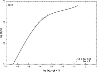
(e)

(f)

Figure 16: Curves of growth (Fe I, Fe II) for the HV 1333 spectra. From left to right, MJD=54785.07912217, MJD=54785.09358357, 54785.10804394

(a)

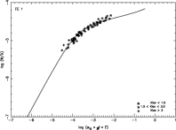
(b)

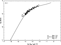
(c)

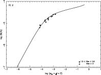
(d)

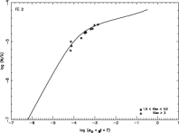
(e)

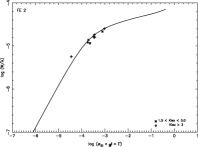
(f)

Figure 17: Curves of growth (Fe I, Fe II) for the HV 1335 spectra. From left to right, MJD=54785.12765152, 54785.14326987, 54785.15889887

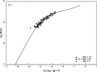
(a)

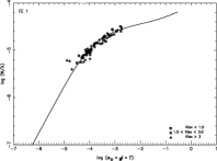
(b)

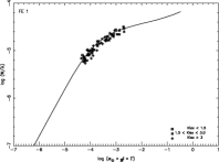
(c)

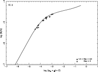
(d)

(e)

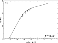
(f)

References

- Allen & Barbuy (2006) Allen, D. M., Barbuy, B., 2006, A&A 454, 895
- Anders & Grevesse (1989) Anders, E., Grevesse, N., 1989, Geochim. Cosmochim. Acta, 53, 1976
- Anderson et al. (2013) Anderson, R. I., Eyer, L., Mowlavi, N., 2013, MNRAS 434, 2238
- Anderson (2014) Anderson, R. I., 2014, A&A 566, L10
- Anderson et al. (2016) Anderson, R. I., Saio, H., Ekström, S., Georgy, C., Meynet, G, 2016, A&A 591, A8
- Andrievsky et al. (2002a) Andrievsky, S. M., Kovtyukh, V. V., Luck, R. E., Lépine, J. R. D., Bersier, D., Maciel, W. J., Barbuy, B., Klochkova, V. G., Panchuk, V. E., Karpischek, R. U., 2002, A&A 381, 32
- Andrievsky et al. (2002b) Andrievsky, S. M., Bersier, D., Kovtyukh, V. V., Luck, R. E., Maciel, W. J., Lépine, J. R. D., Beletsky, Yu. V., 2002, A&A 384, 140
- Andrievsky et al. (2003) Andrievsky, S. M., Egorova, I. A., Korotin, S. A., Kovtyukh, V. V., 2003, AN 324, 532
- Andrievsky et al. (2005) Andrievsky, S. M., Luck, R. E., Kovtyukh, V. V., 2005, AJ 130, 1880
- Andrievsky et al. (2014) Andrievsky, S. M., Luck, R. E., Korotin, S. A., 2014, MNRAS 437, 2106
- Andrievsky et al. (2016) Andrievsky, S. M., Martin, R. P., Kovtyukh, V. V., Korotin, S. A., Lépine, J. R. D., 2016, MNRAS 461, 4256
- Barnes & Evans (1976) Barnes, T. G., Evans, D. S., 1976, MNRAS 174, 489
- Benedict et al. (2007) Benedict, G. F., McArthur, B. E., Feast, M. W., Barnes, T. G., Harrison, T. E., Patterson, R. J., Menzies, J. W., Bean, J. L., Freedman, W. L., 2007, AJ 133, 1810
- Bertelli et al. (2003) Bertelli, G., Nasi, E., Girardi, L., Chiosi, C., Zoccali, M., Gallart, C., 2003, AJ 125, 770
- Bhardwaj et al. (2016) Bhardwaj, A., Kanbur, S. M., Macri, L. M., Singh, H. P., Ngeow, C-C., Wagner-Kaiser, R., Sarajedini, A., 2016, AJ 151, 88
- Bono et al. (1997) Bono, G., Marconi, M., 1997, MNRAS 290, 353
- Bono et al. (2005) Bono, G., Marconi, M., Cassisi, S., Caputo, F., Gieren, W., Pietrzyński, G., 2005 ApJ 621, 966
- Bono et al. (2010) Bono, G., Caputo, F., Marconi, M., Musella, I., 2010, ApJ 715, 277
- Breitfelder et al. (2016) Breitfelder, J., Mérand, A., Kervella, P., Gallenne, A., Szabados, L., Anderson, R. I., Le Bouquin, J.-B., 2016, A&A 587, A117
- Brocato et al. (2004) Brocato, E., Caputo, F., Castellani, V., Marconi, M., Musella, I., 2004 AJ 128, 1597
- Cardelli et al. (1989) Cardelli, J. A., Clayton, G. C., Mathis, J. S., 1989, ApJ 345, 245
- Carrera et al. (2008) Carrera, R., Gallart, C., Aparicio, A., Costa, E., Méndez, R. A., Noël, N. E. D., 2008, AJ 136, 1039,
- Cescutti et al. (2008) Cescutti, G., Matteucci, F., Lanfranchi, G. A., McWilliam, A., 2008, A&A 491, 401
- Chen et al. (2015) Chen, X., de Grijs, R., Deng, L., 2015, MNRAS 446, 1268
- Cioni et al. (2009) Cioni, M.-R. L., 2009, A&A 506, 1137
- Colucci et al. (2011) Colucci, J. E., Bernstein, R. A., Cameron, S. A., McWilliam, A., 2011, ApJ 735, 55
- Colucci et al. (2012a) Colucci, J. E., Bernstein, R. A., Cameron, S. A., McWilliam, A., 2012, ApJ 746, 29
- Colucci et al. (2012b) Colucci, J. E., Bernstein, R. A., 2012 ApJ 749, 124
- Cristallo et al. (2011) Cristallo, S., Piersanti, L., Straniero, O., Gallino, R., Domínguez, I., Abia, C., Di Rico, G., Quintini, M., Bisterzo, S., 2011, ApJS 197, 17
- da Silva et al. (2015) da Silva, R., Milone, André de C., Rocha-Pinto, H. J., 2015, A&A 580, A24
- da Silva et al. (2016) da Silva, R., Lemasle, B., Bono, G., Genovali, K., McWilliam, A., Cristallo, S., Bergemann, M., Buonanno, R., Fabrizio, M., Ferraro, I., François, P., Iannicola, G., Inno, L., Laney, C. D., Kudritzki, R.-P., Matsunaga, N., Nonino, M., Primas, F., Przybilla, N., Romaniello, M., Thévenin, F., Urbaneja, M. A., 2016, A&A 586, A125
- Davies et al. (2015) Davies, B., Kudritzki, R.-P., Gazak, Z., Plez, B., Bergemann, M., Evans, C., Patrick, L., 2015, ApJ 806, 21
- Deb et al. (2015) Deb, S., Singh, H. P., Kumar, S., Kanbur, S. M., 2015, MNRAS 449, 2768
- Dekker et al. (2000) Dekker, H., D’Odorico, S., Kaufer, A., Delabre, B., Kotzlowski, H., 2000, SPIE 4008, 534
- Denissenkov (1994) Denissenkov, P. A., 1994, A&A 287, 113
- Dobbie et al. (2014) Dobbie, P. D., Cole, A. A., Subramaniam, A., Keller, S., 2014, MNRAS 442, 1680
- Efremov (1978) Efremov Iu. N., 1978, SvA 22, 161
- Feast et al. (2012) Feast, M. W., Whitelock, P. A., Menzies, J. W., Matsunaga, N., 2012, MNRAS 421 2998
- Fiorentino et al. (2007) Fiorentino, G., Marconi, M., Musella, I., Caputo, F., 2007, A&A 476, 863
- Fouqué et al. (1997) Fouqué, P., Gieren, W. P., 1997, A&A 320, 799
- Fouqué et al. (2007) Fouqué, P., Arriagada, P., Storm, J., Barnes, T. G., Nardetto, N., Mérand, A., Kervella, P., Gieren, W., Bersier, D., Benedict, G. F., McArthur, B. E., 2007, A&A 476, 73
- Freudling et al. (2013) Freudling, W., Romaniello, M., Bramich, D. M., Ballester, P., Forchi, V., García-Dabló, C. E., Moehler, S., Neeser, M. J., 2013, A&A 559, A96
- Gazak et al. (2015) Gazak, J. Z., Kudritzki, R., Evans, C., Patrick, L., Davies, B., Bergemann, M., Plez, B., Bresolin, F., Bender, R., Wegner, M., Bonanos, A. Z., Williams, S. J., 2015, ApJ 805 182
- Genovali et al. (2013) Genovali, K., Lemasle, B., Bono, G., Romaniello, M., Primas, F., Fabrizio, M., Buonanno, R., François, P., Inno, L., Laney, C. D., Matsunaga, N., Pedicelli, S., Thévenin, F., 2013, A&A 554, A132
- Genovali et al. (2014) Genovali, K., Lemasle, B., Bono, G., Romaniello, M., Fabrizio, M., Ferraro, I., Iannicola, G., Laney, C. D., Nonino, M., Bergemann, M., Buonanno, R., François, P., Inno, L., Kudritzki, R.-P., Matsunaga, N., Pedicelli, S., Primas, F., Thévenin, F., 2014, A&A 566, A37
- Genovali et al. (2015) Genovali, K., Lemasle, B., da Silva, R., Bono, G., Fabrizio, M., Bergemann, M., Buonanno, R., Ferraro, I., François, P., Iannicola, G., Inno, L., Laney, C. D., Kudritzki, R.-P., Matsunaga, N., Nonino, M., Primas, F., Romaniello, M., Urbaneja, M. A., Thévenin, F., 2015, A&A 580, A17
- Gieren et al. (2005) Gieren, W., Storm, J., Barnes, T., G., III, Fouqué, P., Pietrzyński, G., Kienzle, F., 2005, ApJ 627, 224
- Gieren et al. (2013) Gieren, W., Górski, M., Pietrzyński, G., Konorski, P., Suchomska, K., Graczyk, D., Pilecki, B., Bresolin, F., Kudritzki, R.-P., Storm, J., Karczmarek, P., Gallenne, A., Calderón, P., Geisler, D., 2013, ApJ 773, 69
- Glatt et al. (2008) Glatt, K., Grebel, E. K., Sabbi, E., Gallagher, J. S. III, Nota, A., Sirianni, M., Clementini, G., Tosi, M., Harbeck, D., Koch, A., Kayser, A., Da Costa, G., 2008, AJ 136, 1703
- Graczyk et al. (2014) Graczyk, D., Pietrzy/’nski, G., Thompson, I. B., Gieren, W., Pilecki, B., Konorski, P., Udalski, A., Soszy ’nski, I., Villanova, S., Górski, M., Suchomska, K., Karczmarek, P., Kudritzki, R.-P., Bresolin, F., Gallenne, A., 2014, ApJ 780, 59
- Grebel & Brandner (1998) Grebel, E. K., Brandner, W., 1998, in Magellanic Clouds and Other Dwarf Galaxies, edited by T. Richtler, & J. M. Braun, Shaker Verlag, Aachen, 151
- Groenewegen et al. (2008) Groenewegen, M. A. T., 2008, A&A 488, 25
- Groenewegen et al. (2013) Groenewegen, M. A. T., 2013, A&A 550, 70
- Gustafsson et al. (2008) Gustafsson, B., Edvardsson, B., Eriksson, K., Jørgensen, U. G., Nordlund, , Plez, B., 2008 A&A 486, 951
- Haschke et al. (2012a) Haschke, R., Grebel, E. K., Duffau, S., 2012a, AJ 143, 48
- Haschke et al. (2012b) Haschke, R., Grebel, E. K., Duffau, S., 2012b, AJ 144, 107
- Heiter et al. (2015) Heiter, U., Lind, K., Asplund, M., Barklem, P. S., Bergemann, M., Magrini, L., Masseron, T., Mikolaitis, S., Pickering, J. C., Ruffoni, M. P., 2015, Phys. Scr, 90, 054010
- Hill et al. (1995) Hill, V., Andrievsky. S. M., Spite, M., 1995, A&A 293, 347
- Hill et al. (2000) Hill, V., François, P., Spite, M., Primas, F., Spite, F., 2000, A&A 364, 19
- Indebetouw et al. (2005) Indebetouw, R., Mathis, J. S., Babler, B. L., Meade, M. R., Watson, C., Whitney, B. A., Wolff, M. J., Wolfire, M. G., Cohen, M., Bania, T. M., Benjamin, R. A., Clemens, D. P., Dickey, J. M., Jackson, J. M., Kobulnicky, H. A., Marston, A. P., Mercer, E. P., Stauffer, J. R., Stolovy, S. R., Churchwell, E., 2005, ApJ 619, 931
- Inno et al. (2013) Inno, L., Matsunaga, N., Bono, G., Caputo, F., Buonanno, R., Genovali, K., Laney, C. D., Marconi, M., Piersimoni, A. M., Primas, F., Romaniello, M., 2013, ApJ 764, 84
- Inno et al. (2015a) Inno, L., Matsunaga, N., Romaniello, M., Bono, G., Monson, A., Ferraro, I., Iannicola, G., Persson, E., Buonanno, R., Freedman, W., Gieren, W., Groenewegen, M. A. T., Ita, Y., Laney, C. D., Lemasle, B., Madore, B. F., Nagayama, T., Nakada, Y., Nonino, M., Pietrzyński, G., Primas, F., Scowcroft, V., Soszyński, I., Tanabé, T., Udalski, A., 2015a, A&A 576, A30
- Inno et al. (2015b) Inno, L., Bono, G., Romaniello, M., Matsunaga, N., Pietrinferni, A., Genovali, K., Lemasle, B., Marconi, M., Primas, F., 2015 ASPC 491, 265
- Inno et al. (2016) Inno, L., Bono, G., Matsunaga, N., Fiorentino, G., Marconi, M., Lemasle, B., da Silva, R., Soszyński, I., Udalski, A., Romaniello, M., Rix, H.-W., 2016, ApJ 832, 176
- Inno et al. (2017) Inno, L., et al., in prep.
- Jacyszyn-Dobrzeniecka et al. (2016) Jacyszyn-Dobrzeniecka, A. M., Skowron, D. M., Mróz, P., Skowron, J., Soszyński, I., Udalski, A., Pietrukowicz, P., Kozlowski, S., Wyrzykowski, L., Poleski, R., Pawlak, M., Szymański, M. K., Ulaczyk, K., 2016, AcA 66, 149
- Jacyszyn-Dobrzeniecka et al. (2017) Jacyszyn-Dobrzeniecka, A. M., Skowron, D. M., Mróz, P., Soszyński, I., Udalski, A., Pietrukowicz, P., Skowron, J., Poleski, R., Kozlowski, S., Wyrzykowski, L., Pawlak, M., Szymański, M. K., Ulaczyk, K., 2017, AcA 67, 1
- Kato et al. (2007) Kato, D., Nagashima, C., Nagayama, T., et al., 2007, PASJ 59, 6150
- Kervella et al. (2004) Kervella, P., Nardetto, N., Bersier, D., Mourard, D., Coudé du Foresto, V., 2004, A&A 416, 941
- Kervella et al. (2017) Kervella, P., Trahin, B., Bond, H. E., Gallenne, A., Szabados, L., Mérand, A., Breitfelder, J., Dailloux, J., Anderson, R. I., Fouqué, P., Gieren, W., Nardetto, N., Pietrzyński, G., 2017, A&A 600, A127
- Kewley et al. (2008) Kewley, L. J., Ellison, S. L., 2008, ApJ 681, 1183
- Korotin et al. (2014) Korotin, S. A., Andrievsky, S. M., Luck, R. E., Lépine, J. R. D., Maciel, W. J., Kovtyukh, V. V., 2014, MNRAS 444, 3301
- Kovtyukh & Andrievsky (1999) Kovtyukh, V. V., Andrievsky, S. M., 1999, A&A 351, 597
- Kovtyukh & Gorlova (2000) Kovtyukh, V. V., Gorlova, N. I., 2000, A&A 358, 587
- Kovtyukh et al. (2005) Kovtyukh, V. V., Wallerstein, G., Andrievsky, S. M., 2005, PASP 117, 1173
- Kupka et al. (1999) Kupka, F., Piskunov, N. E., Ryabchikova, T. A., Stempels, H. C., Weiss, W. W., 1999, A&AS, 138, 119
- Lemasle et al. (2007) Lemasle, B., François, P., Bono, G., Mottini, M., Primas, F., Romaniello, M., 2007, A&A 467, 283
- Lemasle et al. (2008) Lemasle, B., François, P., Piersimoni, A. Pedicelli, S., Bono, G., Laney, C. D., Primas, F., Romaniello, M., 2008, A&A 490, 613
- Lemasle et al. (2013) Lemasle, B., François, P., Genovali, K., Kovtyukh, V. V., Bono, G., Inno, L., Laney, C. D., Kaper, L., Bergemann, M., Fabrizio, M., Matsunaga, N., Pedicelli, S., Primas, F., Romaniello, M., 2013, A&A 558, A31
- Lind et al. (2011) Lind, K., Asplund, M., Barklem, P. S., Belyaev, A. K., 2011, A&A 528, 103
- Luck & Lambert (1985) Luck, R. E., Lambert, D. L., 1985, ApJ 298, 782
- Luck & Lambert (1992) Luck, R. E., Lambert, D. L., 1992, ApJS 79, 303
- Luck et al. (1998) Luck, R. E., Moffett, T. J., Barnes, T. G. III, Gieren, W. P., 1998, AJ 115, 605
- Luck et al. (2003) Luck, R. E., Gieren, W. P., Andrievsky, S. M., Kovtyukh, V. V., Fouqué, P., Pont, P., Kienzle, F., 2003, A&A 401, 939
- Luck et al. (2011) Luck, R. E.; Andrievsky, S. M., Kovtyukh, V. V., Gieren, W., Graczyk, D., 2011, AJ 142, 51
- Luck & Lambert (2011) Luck, R. E., Lambert, D. L., 2011, AJ 142, 136
- Madore (1982) Madore, B. F., 1982, ApJ 253, 575
- Majaess et al. (2013) Majaess, D., Carraro, G., Moni Bidin, C., Bonatto, C., Berdnikov, L., Balam, D., Moyano, M., Gallo, L., Turner, D., Lane, D., Gieren, W., Borissova, J., Kovtyukh, V., Beletsky, Y., 2013, A&A 560, A22
- Marconi et al. (2013) Marconi, M., Molinaro, R., Ripepi, V., Musella, I., Brocato, E., 2013, MNRAS 428 2185
- Marconi et al. (2017) Marconi, M., Molinaro, R., Ripepi, V., Cioni, M.-R. L., Clementini, G., Moretti, M. I., Ragosta, F., de Grijs, R., Groenewegen, M. A. T., Ivanov, V. D., 2017, MNRAS 466, 3206
- Martin et al. (2015) Martin, R. P., Andrievsky, S. M., Kovtyukh, V. V., Korotin, S. A., Yegorova, I. A., Saviane, I., 2015, MNRAS 449, 4071
- McWilliam et al. (2003) McWilliam, A., Rich, R. M., Smecker-Hane, T. A., 2003, ApJ 592, L21
- Mérand et al. (2015) Mérand, A., Kervella, P., Breitfelder, J., Gallenne, A., Coudé du Foresto, V., ten Brummelaar, T. A., McAlister, H. A., Ridgway, S., Sturmann, L., Sturmann, J., Turner, N. H., 2015, A&A 584, A80
- Milone et al. (2013) Milone, A. P., Bedin, L. R., Cassisi, S., Piotto, G., Anderson, J., Pietrinferni, A., Buonanno, R., 2013, A&A 555, A143
- Milone et al. (2017) Milone, A. P., Marino, A. F., D’Antona, F., Bedin, L. R., Piotto, G., Jerjen, H., Anderson, J., Dotter, A., Di Criscienzo, M., Lagioia, E. P., 2017, MNRAS 465, 4363
- Molinaro et al. (2012) Molinaro, R., Ripepi, V., Marconi, M., Musella, I., Brocato, E., Mucciarelli, A., Stetson, P. B., Storm, J., Walker, A. R., 2012, ApJ 748, 69
- Monson et al. (2012) Monson, A. J., Freedman, W. L., Madore, B. F., Persson, S. E., Scowcroft, V., Seibert, M., Rigby, J. R., 2012, ApJ 759, 146
- Mourard et al. (1997) Mourard, D., Bonneau, D., Koechlin, L., Labeyrie, A., Morand, F., Stee, P., Tallon-Bosc, I., Vakili, F., 1997, A&A 317, 789
- Mucciarelli et al. (2011) Mucciarelli, A., Cristallo, S., Brocato, E., Pasquini, L., Straniero, O., Caffau, E., Raimondo, G., Kaufer, A., Musella, I., Ripepi, V., Romaniello, M., Walker, A. R., 2011, MNRAS 413, 837
- Musella et al. (2016) Musella, I., Marconi, M., Stetson, P. B., Raimondo, G., Brocato, E., Molinaro, R., Ripepi, V., Carini, R., Coppola, G., Walker, A. R., Welch, D. L., 2016, MNRAS 457, 3084
- Nardetto et al. (2011) Nardetto, N., Fokin, A., Fouqué, P., Storm, J., Gieren, W., Pietrzynski, G., Mourard, D., Kervella, P., 2011, A&A 534, 16
- Nardetto et al. (2014) Nardetto, N., Poretti, E., Rainer, M., Guiglion, G., Scardia, M., Schmid, V. S., Mathias, P., 2014, A&A 561, A151
- Neilson et al. (2012) Neilson, H. R., Nardetto, N., Ngeow, C-C., Fouqué, P., Storm, J., 2012, A&A 541, A134
- Ngeow et al. (2012) Ngeow, C-C., Citro, D. M., Kanbur, S. M., 2012, MNRAS 420, 585
- Ngeow et al. (2015) Ngeow, C-C., Sarkar, S., Bhardwaj, A., Kanbur, S. M., Singh, H. P., 2015, ApJ 813, 57
- Nidever et al. (2013) Nidever, D. L., Monachesi, A., Bell, E. F., Majewski, S. R., Muñoz, R. R., Beaton, R. L., 2013, ApJ 779, 145
- North et al. (2012) North, P., Cescutti, G., Jablonka, P., Hill, V., Shetrone, M., Letarte, B., Lemasle, B., Venn, K. A., Battaglia, G., Tolstoy, E., Irwin, M. J., Primas, F., François, P., 2012, A&A 541, A45
- Parisi et al. (2015) Parisi, M. C., Geisler, D., Clariá, J. J., Villanova, S., Marcionni, N., Sarajedini, A., Grocholski, A. J., 2015, AJ 149, 154
- Parisi et al. (2016) Parisi, M. C., Geisler, D., Carraro, G., Clariá, J. J., Villanova, S., Gramajo, L. V., Sarajedini, A., Grocholski, A. J., 2016, AJ 152, 58
- Pasquini et al. (2002) Pasquini, L., Avila, G., Blecha, A., Cacciari, C., Cayatte, V., Colless, M., Damiani, F., de Propris, R., Dekker, H., di Marcantonio, P., Farrell, T., Gillingham, P., Guinouard, I., Hammer, F., Kaufer, A., Hill, V., Marteaud, M., Modigliani, A., Mulas, G., North, P., Popovic, D., Rossetti, E., Royer, F., Santin, P., Schmutzer, R., Simond, G., Vola, P., Waller, L., Zoccali, M., 2002, Msngr 110, 1
- Patrick et al. (2015) Patrick, L. R., Evans, C. J., Davies, B., Kudritzki, R.-P., Gazak, J. Z., Bergemann, M., Plez, B., Ferguson, A. M. N., 2015, ApJ 803, 14
- Pedicelli et al. (2010) Pedicelli, S., Lemasle, B., Groenewegen, M., Romaniello, M., Bono, G., Laney, D., François, P.,M., Buonanno, R., Caputo, F.,Lub, J., Pel, J. W., Primas, F., Pritchard, J., 2010, A&A 518, A11
- Pilyugin et al. (2016) Pilyugin, L. S., Grebel, E. K., 2016, MNRAS 457, 3678
- Prochaska et al. (2000) Prochaska, J. X., Naumov, S. O., Carney, B. W., McWilliam, A., Wolfe, A. M., 2000, AJ 120, 2513
- Rich et al. (2014) Rich, J. A., Persson, S. E., Freedman, W. L., Madore, B. F., Monson, A. J., Scowcroft, V., Seibert, M., 2014, ApJ 794, 107
- Ripepi et al. (2012) Ripepi, V., Moretti, M. I., Marconi, M., Clementini, G., Cioni, M.-R. L., Marquette, J. B., Girardi, L., Rubele, S., Groenewegen, M. A. T., de Grijs, R., Gibson, B. K., Oliveira, J. M., van Loon, J. Th., Emerson, J. P., 2012, MNRAS 424, 1807
- Romaniello et al. (2005) Romaniello, M., Primas, F., Mottini, M, Groenewegen, M., Bono, G., François, P., 2005, A&A 429, 37
- Romaniello et al. (2008) Romaniello, M., Primas, F., Mottini, M., Pedicelli, S., Lemasle, B., Bono, G., François, P., Groenewegen, M. A. T., Laney, C. D., 2008, A&A 488, 731
- Sasselov (1986) Sasselov, D. D., 1986, PASP 98, 561
- Scowcroft et al. (2013) Scowcroft, V., Freedman, W., L., Madore, B. F., Monson, A. J., Persson, S. E., Seibert, M., Rigby, J. R., Melbourne, J., 2013, ApJ 773, 106
- Scowcroft et al. (2016) Scowcroft, V., Freedman, W., L., Madore, B. F., Monson, A. J., Persson, S. E., Rich, J., Seibert, M., Rigby, J. R., 2016 ApJ 816, 49S
- Skowron et al. (2016) Skowron, D. M., Soszyński, I., Udalski, A., Szymański, M. K., Pietrukowicz, P., Skowron, J., Poleski, R., Wyrzykowski, L., Ulaczyk, K., Kozłowski, S., Mróz, P., Pawlak, M., 2016, AcA 66, 269
- Skrutskie et al. (2006) Skrutskie, M. F., Cutri, R. M., Stiening, R., Weinberg, M. D., Schneider, S., Carpenter, J. M., Beichman, C., Capps, R., Chester, T., Elias, J., Huchra, J., Liebert, J., Lonsdale, C., Monet, D. G., Price, S., Seitzer, P., Jarrett, T., Kirkpatrick, J. D., Gizis, J. E., Howard, E., Evans, T., Fowler, J., Fullmer, L., Hurt, R., Light, R., Kopan, E. L., Marsh, K. A., McCallon, H. L., Tam, R., Van Dyk, S., Wheelock, S., 2006, AJ 131, 1163
- Soszyński et al. (2010) Soszyński, I., Poleski, R., Udalski, A., Szymański, M. K., Kubiak, M., Pietrzyński, G., Wyrzykowski, L., Szewczyk, O., Ulaczyk, K., 2010, AcA 60, 17
- Soubiran & Girard (2005) Soubiran, C., Girard, P., 2005, A&A 438, 139
- Spite (1967) Spite, M., 1967, AnAp 30 211
- Spite et al. (1989) Spite, F., Spite, M., François, P., 1989, A&A 210, 25
- Stetson & Pancino (2008) Stetson, P. B., Pancino, E.. 2008, PASP, 120, 1332
- Storm et al. (2004a) Storm, J., Carney, B. W., Gieren, W. P., Fouqué, P., Freedman, W. L., Madore, B. F., Habgood, M. J., 2004, A&A 415, 521
- Storm et al. (2004b) Storm, J., Carney, B. W., Gieren, W. P., Fouqué, P., Latham, D. W., Fry, A. M., 2004, A&A 415, 531
- Storm et al. (2005) Storm, J., Gieren, W. P., Fouqué, P., Barnes, T. G., III, Gómez, M., 2005, A&A 440, 487
- Storm et al. (2011a) Storm, J., Gieren, W., Fouqué, P., Barnes, T. G., Pietrzyński, G., Nardetto, N., Weber, M., Granzer, T., Strassmeier, K. G., 2011, A&A 534, 94
- Storm et al. (2011b) Storm, J., Gieren, W., Fouqué, P., Barnes, T. G., Soszyński, I., Pietrzyński, G., Nardetto, N., Queloz, D., 2011, A&A 534, 95
- Subramanian et al. (2012) Subramanian, S., Subramaniam, A., 2012, ApJ 744, 128
- Szabados (2003) Szabados, L., 2003, Inf. Bull. Var. Stars, No. 5394
- Szabados & Nehéz (2012) Szabados, L., Nehź, D., 2012, MNRAS 426 3148
- Takeda et al. (2013) Takeda, Y., Kang, D.-I., Han, I., Lee, B.-C., Kim, K.-M., 2013, MNRAS 432, 769
- Turner (2010) Turner, D. G., 2010, Ap&SS 326, 219
- Turner et al. (2012) Turner, D. G., Majaess, D. J., Lane, D. J., Balam, D. D., Gieren, W. P., Storm, J., Forbes, D. W., Havlen, R. J., Alessi, B., 2012, MNRAS 422, 2501
- Udalski et al. (2015) Udalski, A., Szymanski, M. K., Szymanski, G., 2015, AcA 65, 1
- van der Marel & Cioni (2001) van der Marel, R. P., Cioni, M.-R. L., 2001, AJ 122, 1807
- Van der Swaelmen et al. (2013) Van der Swaelmen, M., Hill, V., Primas, F., Cole, A. A., 2013, A&A 560, A44
- van Leeuwen et al. (2007) van Leeuwen, F., Feast, M. W., Whitelock, P. A., Laney, C. D., 2007, MNRAS 379, 723
- Weinberg & Nikolaev (2001) Weinberg, M. D., Nikolaev, S., 2001, ApJ 548, 712
- Welch et al. (1991) Welch, D. L., Mateo, M., Côté, P., Fischer, P., Madore, B. F., 1991, AJ 101, 490
- Welch & Stetson (1993) Welch, D. L., Stetson, P. B., 1993 AJ 105, 1813
- Welch (1994) Welch, D.L., 1994, AJ 108, 1421
- Wesselink (1969) Wesselink, A. J., 1969, MNRAS 144, 297
- Yong et al. (2006) Yong, D., Carney, B. W., Teixera de Almeida, M. L., Pohl, B. L., 2006, AJ 131, 2256