Optimal Sensor Design and Zero-Delay Source Coding for Continuous-Time Vector Gauss-Markov Processes

Abstract

We consider the situation in which a continuous-time vector Gauss–Markov process is observed through a vector Gaussian channel (sensor) and estimated by the Kalman–Bucy filter. Unlike in standard filtering problems where a sensor model is given a priori, we are concerned with the optimal sensor design by which (i) the mutual information between the source random process and the reproduction (estimation) process is minimized, and (ii) the minimum mean-square estimation error meets a given distortion constraint. We show that such a sensor design problem is tractable by semidefinite programming. The connection to zero-delay source-coding is also discussed.

I Introduction

In this paper, we consider a situation in which a continuous-time vector Gauss–Markov process (the source random process) is estimated by the Kalman–Bucy filter based on the output of a memoryless vector Gaussian channel (the sensor). We study this estimation mechanism from the perspectives of (i) the mean-square error (MSE) between the source and the estimate, and (ii) the mutual information rate between the source and the estimate. From standard rate–distortion theory, it is intuitively clear that an accurate sensing mechanism should lead to a small MSE and a large mutual information, while a noisy sensing mechanism implies a large MSE and a small mutual information. In this paper, we make this intuition explicit by deriving a trade-off curve between these two metrics by constructing trade-off achieving sensor gain matrices. In particular, we show that trade-off achieving sensor gain matrices are easily computed by semidefinite programming, and consequently the trade-off curve admits a convenient semidefinite representation.

There is a simple and explicit relationship (often called the I-MMSE relationship in the literature) between the mutual information (I) and the minimum mean-square error (MMSE) when a random variable is observed through a Gaussian channel. Guo et al. [1] showed that the derivative of the mutual information with respect to the channel SNR (signal-to-noise ratio) is equal to half the MMSE. They also considered causal estimation of random processes through Gaussian channels and provided a remarkably simple connection between causal and non-causal MMSE. For continuous-time source processes observed through Gaussian channels, Duncan [2] already derived a relevant result, stating that “twice the mutual information is merely the integration of the trace of the optimal mean square filtering error.” Kadota et al. [3] considered estimation of continuous-time source over Gaussian channel with feedback (the source is causally affected by channel output). Weissman et al. [4] further studied the cases with feedback, where a fundamental relationship between directed information and MMSE is derived.

In parallel with the I-MMSE formulas for Gaussian observations, there exists a line of research for random processes observed through Poisson channels. Guo et al. [5] studied a relationship between mutual information and the estimation error, measured by the mean value of the logarithm of the ratio of the channel input plus dark current and its mean estimate. Remarkably, the same formula as the I-MMSE relationship for Gaussian case is recovered for Poisson cases as well, provided that MMSE is replaced by a suitable loss function for Poisson channels [6]. Estimation of continuous-time processes through Poisson channels with feedback is studied by [7, 4]. Recently, an overarching theory unifying the I-MMSE relationship for Gaussian channels and the similar relationship for Poisson channels is proposed [8].

Applications of the I-MMSE formula can be found in channel coding problems. Palomar and Verdú [9] extended the result by [1] to vector Gaussian channels, where an explicit formula relating gradients of mutual information with respect to channel parameters and estimate covariance matrices is obtained. Based on this result, they proposed a gradient ascent algorithm for channel precoder design where input-output mutual information is maximized subject to input power constraints.

In this paper, we apply Duncan’s I-MMSE formula for the aforementioned trade-off study. Our study is motivated by the zero-delay source coding problem. Derpich and Østergaard [10] showed that minimum the data-rate achievable by zero-delay source coding of a Gaussian source subject to a quadratic distortion constraint is closely approximated by the zero-delay rate-distortion function (also called sequential- or non-anticipative rate-distortion function in the literature). For Gauss–Markov sources with mean-square distortion criteria, computation of zero-delay rate-distortion functions and construction of optimal test channels are addressed by recent literature [11, 12]. Stavrou et al. [11] showed that the optimal test channel can be realized by a memoryless Gaussian channel (sensor) with feedback and a Kalman filter. Tanaka et al. [12] presented a different realization of the test channel, using a memoryless Gaussian channel without feedback and a Kalman filter. The latter observation implies that the zero-delay rate-distortion function can be computed by considering the I-MMSE trade-off with respect to the Gaussian channel gain (sensor gain matrix) [12]. The I-MMSE trade-off in the present paper can be viewed as a continuous-time counterpart of a similar trade-off considered in discrete-time [12]. From analogous discrete-time results, it is conjectured that results in this paper provide fundamental performance limitations of zero-delay source coding schemes for continuous-time sources, although zero-delay source coding problems for continuous-time sources are not fully explored in the literature.

This paper is organized as follows. Problem formulation is presented in Section II. Section III summarizes the main result. A connection to zero-delay source coding problem is discussed in Section IV. Section V summarizes the paper and discuss future work.

Notation: Let $(\Omega,\mathcal{F},\mathcal{P})$ be a probability space and let $X$ be a random variable in a measurable space $(\mathcal{X},\mathcal{A})$. The probability distribution $\mu_{X}$ of $X$ is defined by

$$\mu_{X}(A)=\mathcal{P}\{\omega:X(\omega)\in A\}\;\;\forall A\in\mathcal{A}.$$

If $X$ and $Y$ are random variables in the same measurable space with distributions $\mu_{X}$ and $\mu_{Y}$, the relative entropy from $Y$ to $X$ is defined by

$$D(\mu_{X}\|\mu_{Y})=\int\log\frac{d\mu_{X}}{d\mu_{Y}}d\mu_{X}$$

if the Radon-Nikodym derivative $\frac{d\mu_{X}}{d\mu_{Y}}$ exists. If random variables $X$ and $Y$ have a joint probability distribution $\mu_{XY}$, the mutual information between $X$ and $Y$ is defined by

$$I(X;Y)=D(\mu_{XY}\|\mu_{X}\otimes\mu_{Y})$$

where $\mu_{X}\otimes\mu_{Y}$ is the product measure defined by the marginal distributions. If $\mu_{X}$ is discrete, the entropy of $X$ is defined by

$$H(X)=-\sum_{x\in\mathcal{X}}\mu_{X}(x)\log\mu_{X}(x).$$

II Problem Formulation

Let $(\Omega,\mathcal{F},\mathcal{P})$ be a complete probability space and $\mathcal{F}_{t}\subset\mathcal{F}$ be a non-decreasing family of $\sigma$-algebras. Let $(W_{t},\mathcal{F}_{t})$ and $(V_{t},\mathcal{F}_{t})$ be $n$-dimensional independent standard Wiener processes with respect to $\mathcal{P}$. Assume that the source random process is an $n$-dimensional Gauss–Markov process of the form

$$dX_{t}=AX_{t}dt+BdW_{t},\;\;t\in[0,\infty)$$ (1)

with $X_{0}=0$. The source process is observed through an $n$-dimensional Gaussian channel (or sensor):

$$dY_{t}=CX_{t}dt+dV_{t},\;\;t\in[0,\infty)$$ (2)

with $Y_{0}=0$. We assume that $(A,B)$ is a controllable pair.

II-A Minimum mean-square error (MMSE) estimate

Let $\mathcal{F}_{t}^{Y}\subset\mathcal{F}$ be the $\sigma$-algebra generated by $Y_{s},0\leq s\leq t$. Denote by $\hat{X}_{t}\triangleq\mathbb{E}(X_{t}|\mathcal{F}_{t}^{Y})$ the causal MMSE estimate of the process (1) via the observation (2), calculated by the Kalman–Bucy filter

$$d\hat{X}_{t}=A\hat{X}_{t}dt+P_{t}C^{\top}(dY_{t}-C\hat{X}_{t}dt),\;\;t\in[0,\infty)$$ (3)

with $\hat{X}_{0}=0$. In (3), $P_{t}$ is the unique solution to the matrix Riccati differential equation

$$\frac{dP_{t}}{dt}=AP_{t}+P_{t}A^{\top}-P_{t}C^{\top}CP_{t}+BB^{\top},\;\;t\in[0,\infty)$$ (4)

with $P_{0}=0$.

For notational simplicity, we denote by $X_{0}^{T}$, $Y_{0}^{T}$, $\hat{X}_{0}^{T}$ the random processes $X_{t}$, $Y_{t}$, $\hat{X}_{t}$ over the horizon $0\leq t\leq T$ as defined above. The MMSE performance over the considered horizon is denoted by

$$\rho(X_{0}^{T},\hat{X}_{0}^{T})\triangleq\int_{0}^{T}\mathbb{E}\|X_{t}-\hat{X}_{t}\|^{2}dt=\int_{0}^{T}\text{Tr}(P_{t})\;dt.$$

II-B Mutual information

We are also interested in the mutual information $I(X_{0}^{T};\hat{X}_{0}^{T})$ between $X_{0}^{T}$ and $\hat{X}_{0}^{T}$.

Theorem 1

Let the random processes $X_{0}^{T}$ and $\hat{X}_{0}^{T}$ be defined as above. Then

$$I(X_{0}^{T};\hat{X}_{0}^{T})=\frac{1}{2}\int_{0}^{T}\mathbb{E}\|C(X_{t}-\hat{X}_{t})\|^{2}dt.$$

Proof:

Set $Z_{t}=CX_{t}$. The following identity is well-known (e.g., Duncan [2]):

$$I(Y_{0}^{T};Z_{0}^{T})=\frac{1}{2}\int_{0}^{T}\mathbb{E}\|C(X_{t}-\hat{X}_{t})\|^{2}dt.$$ (5)

For completeness, a proof of (5) is given in Appendix A. We also have an identity

$$I(Y_{0}^{T};Z_{0}^{T})=I(Y_{0}^{T};X_{0}^{T}),$$ (6)

whose proof is provided in Appendix B.

Due to the property of the Kalman–Bucy filter, $\hat{X}_{0}^{T}$ is a sufficient statistic of $X_{0}^{T}$ for $Y_{0}^{T}$. Thus

$$I(X_{0}^{T};Y_{0}^{T})=I(X_{0}^{T};\hat{X}_{0}^{T}).$$ (7)

The claim follows from (5)–(7). ∎

It is immediate from Theorem 1 that the mutual information of interest can be written in terms of the solution $P_{t}$ to the Riccati equation (4) as

$$I(X_{0}^{T};\hat{X}_{0}^{T})=\frac{1}{2}\int_{0}^{T}\text{Tr}(CP_{t}C^{\top})dt.$$

II-C I-MMSE trade-off via observation channel design

In this paper, we construct the optimal observation gain $C\in\mathbb{R}^{n\times n}$ in the observation channel (2) that minimizes the average mutual information while the average MMSE is smaller than a given constant $D$. Formally, we seek an optimal solution to the problem

$$R(D)\triangleq\inf_{C\in\mathcal{C}}\;\;\; \limsup_{T\rightarrow+\infty}\frac{1}{T}I(X_{0}^{T};\hat{X}_{0}^{T})$$ (8a)

s.t. $$\limsup_{T\rightarrow+\infty}\frac{1}{T}\rho(X_{0}^{T},\hat{X}_{0}^{T})\leq D.$$ (8b)

In (8), the underlying linear system model (1) is given. The domain of optimization $\mathcal{C}\subset\mathbb{R}^{n\times n}$ is the set of matrices $C$ such that $(A,C)$ is a detectable pair, i.e., $A+LC$ is Hurwitz stable for some matrix $L$. Below, we show that there exists an optimal solution and thus “inf” can be replaced by “min.”

III Main Result

We first assume that a precoder matrix $C\in\mathcal{C}$ is given. Since we assume $(A,B)$ is controllable and $(A,C)$ is detectable, the algebraic Riccati equation

$$AP+PA^{\top}-PC^{\top}CP+BB^{\top}=0$$ (9)

admits a unique positive definite solution $P$ [13, Theorem 13.7, Corollary 13.8]. Under the same assumption, the solution $P_{t}$ to the Riccati differential equation (4) with $P_{0}=0$ satisfies $P_{t}\rightarrow P$ as $t\rightarrow+\infty$ (e.g., [14, Theorem 10.10]), where $P$ is the unique positive definite solution to (9). Thus, it follows from the convergence of Cesàro mean that

$$\frac{1}{T}I(Y_{0}^{T};Z_{0}^{T}) =\frac{1}{2T}\int_{0}^{T}\text{Tr}(CP_{t}C^{\top})dt\rightarrow\frac{1}{2}\text{Tr}(CPC^{\top})$$

$$\frac{1}{T}\rho(X_{0}^{T},\hat{X}_{0}^{T}) =\frac{1}{T}\int_{0}^{T}\text{Tr}(P_{t})dt\rightarrow\text{Tr}(P)\;\;\text{ as }T\rightarrow+\infty.$$

Hence, the right hand side of (8) can be written as

$$\inf_{C\in\mathcal{C},P\succ 0}\;\; \frac{1}{2}\text{Tr}(CPC^{\top})$$ (10a)

s.t. $$AP+PA^{\top}-PC^{\top}CP+BB^{\top}=0$$ (10b)

$$\text{Tr}(P)\leq D.$$ (10c)

Now we show that the optimization problem (10) is reformulated as a semidefinite programming problem. First, under the equality constraint (10b), the objective function can be written as

$$\frac{1}{2}\text{Tr}(CPC^{\top}) =\frac{1}{2}\text{Tr}(PC^{\top}CPP^{-1})$$ (11a)

$$=\text{Tr}(A)+\frac{1}{2}\text{Tr}(B^{\top}P^{-1}B)$$ (11b)

$$=\min_{Q}\;\;\;\text{Tr}(A)+\frac{1}{2}\text{Tr}(Q)$$ (11c)

$$\hskip 15.0694pt\text{s.t.}\;\;\;B^{\top}P^{-1}B\preceq Q$$

$$=\min_{Q}\;\;\;\text{Tr}(A)+\frac{1}{2}\text{Tr}(Q)$$ (11d)

$$\hskip 15.0694pt\text{s.t.}\;\;\;\left[\begin{array}[]{cc}Q&B^{\top}\!\!\\ B&\!\!P\end{array}\right]\succeq 0.$$ (11g)

The equality constraint (10b) is used to obtain (11b) from (11a). Equality (11c) holds since the unique solution to the minimization problem in (11c) is $Q=B^{\top}P^{-1}B$. We have applied the Schur complement formula in (11d).

The next lemma allows us to replace the nonlinear equality constraint (10b) with a linear inequality constraint.

Lemma 1

If $(A,B)$ is controllable, then the following conditions are equivalent.

• $\exists C\in\mathcal{C},P\succ 0\text{ s.t. }AP+PA^{\top}-PC^{\top}CP+BB^{\top}=0.$

• $\exists P\succ 0\text{ s.t. }AP+PA^{\top}+BB^{\top}\succeq 0.$

Proof:

The direction (i)$\Rightarrow$(ii) is trivial. To show (ii)$\Rightarrow$(i), notice that if condition (ii) holds, then clearly there exists a matrix $C$ such that

$$AP+PA^{\top}-PC^{\top}CP+BB^{\top}=0.$$ (12)

To complete the proof, we show that for every $C$ satisfying (12), $(A,C)$ is a detectable pair. It is sufficient to show that $A-PC^{\top}C$ is stable. To this end, rewrite (12) as

$$(A-PC^{\top}\!C)P+P(A-PC^{\top}\!C)^{\top}\!\!+PC^{\top}\!CP+BB^{\top}\!\!=\!0$$ (13)

and suppose that $(A-PC^{\top}\!C)^{\top}$ is not stable. Let $\lambda$ be an unstable eigenvalue and $x$ be the corresponding eigenvector:

$$(A^{\top}-C^{\top}CP)x=\lambda x.$$ (14)

Pre- and post-multiplying (13) by $x^{*}$ and $x$, we have

$$(\lambda+\bar{\lambda})x^{*}Px+x^{*}(PC^{\top}CP+BB^{\top})x=0.$$

Since $\text{Re}(\lambda)\geq 0$ and $P\succ 0$, this implies $CPx=0$ and $B^{\top}x=0$. Thus, from (14), we obtain $A^{\top}x=\lambda x$ and $B^{\top}x=0$. This contradicts the Popov-Belevitch-Hautus (PBH) test for controllability of $(A,B)$. ∎

Applying (11) and Lemma 1 to (10), we obtain the following result,

$$R(D)=\inf_{P\succ 0,Q} \;\;\text{Tr}(A)+\frac{1}{2}\text{Tr}(Q)$$ (15a)

s.t. $$\;AP+PA^{\top}+BB^{\top}\succeq 0$$ (15b)

$$\left[\begin{array}[]{cc}Q&B^{\top}\!\!\\ B&\!\!P\end{array}\right]\succeq 0$$ (15e)

$$\;\;\text{Tr}(P)\leq D.$$ (15f)

The main result of this paper is given by the next theorem.

Theorem 2

Suppose $(A,B)$ is controllable. The optimal value $R(D)$ of (8) admits a semidefinite representation

$$R(D)=\min_{P\succ 0,Q} \;\;\text{Tr}(A)+\frac{1}{2}\text{Tr}(Q)$$

s.t. $$\;AP+PA^{\top}+BB^{\top}\succeq 0$$

$$\left[\begin{array}[]{cc}Q&B^{\top}\!\!\\ B&\!\!P\end{array}\right]\succeq 0$$

$$\;\;\text{Tr}(P)\leq D.$$

In particular, there exists an optimal solution $P\succ 0$, $Q\succeq 0$ attaining the optimal value. Moreover, any matrix $C\in\mathcal{C}$ satisfying

$$AP+PA^{\top}-PC^{\top}CP+BB^{\top}=0,$$

which always exists, is an optimal solution to (8).

Proof:

Since we have (15), it is left to show that the optimal value is attained. By continuity, $\inf_{P\succ 0,Q}$ in (15) can be replaced with $\inf_{P\succeq 0,Q}$ without changing the optimal value. After this replacement, the existence of an optimal solution is guaranteed by Weierstrass’ theorem [15, Proposition A.8], since the feasible domain for $(P,Q)$ is closed and the objective function is coercive. Thus $\inf_{P\succeq 0,Q}$ can be written as $\min_{P\succeq 0,Q}$:

$$R(D)=\min_{P\succeq 0,Q} \;\;\text{Tr}(A)+\frac{1}{2}\text{Tr}(Q)$$ (16a)

s.t. $$\;AP+PA^{\top}+BB^{\top}\succeq 0$$ (16b)

$$\left[\begin{array}[]{cc}Q&B^{\top}\!\!\\ B&\!\!P\end{array}\right]\succeq 0$$ (16e)

$$\;\;\text{Tr}(P)\leq D.$$ (16f)

Now, we show that if $(P,Q)$ is an optimal solution to (16), then $P$ is nonsingular. To show this by contradiction, assume $P\succeq 0$ is singular. Without loss of generality, assume

$$P=\left[\begin{array}[]{cc}P_{1}&0\\ 0&0\end{array}\right]\text{ with }P_{1}\succ 0.$$

Also, consider a corresponding partitioning of $A$ and $B$:

$$A=\left[\begin{array}[]{cc}A_{11}&A_{12}\\ A_{21}&A_{22}\end{array}\right],B=\left[\begin{array}[]{c}B_{1}\\ B_{2}\end{array}\right].$$

First, if $(P,Q)$ is a feasible solution to (16), then it must be that $\text{Im}(B)\subseteq\text{Im}(P)$. To see this by contradiction, suppose there exists a matrix $N$ such that $NB\neq 0$ and $NP=0$. Then, pre- and post-multiplying (16e) by $\text{diag}(I,N)$ and $\text{diag}(I,N^{\top})$, we obtain

$$\left[\begin{array}[]{cc}Q\!&B^{\top}N^{\top}\\ NB&\!0\end{array}\!\right]\succeq 0.$$

However, this is a contradiction because a matrix of this structure with non-zero off-diagonal entries must be indefinite. Thus, we conclude that $\text{Im}(B)\subseteq\text{Im}(P)$ and $B_{2}=0$.

Next, it must be that $A_{21}\neq 0$ since otherwise

$$\text{dim}(\text{Im}[\;B\;\;AB\;\;A^{2}B\;\;...\;\;A^{n-1}B\;])<n$$

which contradicts the controllability of $(A,B)$.

Finally, with the above observations, (16a) becomes

$$\left[\begin{array}[]{cc}A_{11}P_{1}+P_{1}A_{11}^{\top}+B_{1}B_{1}^{\top}\!&P_{1}A_{21}^{\top}\\ A_{21}P_{1}&0\end{array}\!\right]\succeq 0$$

which is again a contradiction since off-diagonal matrices are non-zero. Thus, we conclude that if $(P,Q)$ is an optimal solution to (16), then $P$ is nonsingular. ∎

IV Application

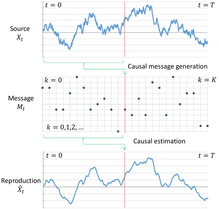
Figure 1: Zero delay source coding of continuous-time signal.

In this section, we consider an application of the optimization problem (8) to a zero-delay source coding scenario depicted in Fig. 1.

Let $X_{t}$ be a continuous-time source random process (e.g., video). The source process is encoded with sampling period $\tau=\frac{T}{K}$, and a sequence of codewords $m_{k}=e_{k}(X_{0}^{k\tau})$, $k=1,2,...,K$ is generated. We assume $m_{0}=0$. For each $k=1,2,...,K$, we assume that $e_{k}$ is a $\mathbb{Z}^{n}$-valued map whose domain is the space of sample paths $X_{t}$, $0\leq t\leq k\tau$. A simple example is $n$ parallel scalar quantizers with uniform quantizer step sizes $\Delta=(\Delta_{1},...,\Delta_{n})$:

$$(m_{k})_{i}=\lfloor\Delta_{i}(X_{k\tau})_{i}\rfloor,\forall i=1,2,...,n.$$

Introduce a continuous-time process $M_{t}=m_{\lfloor\frac{t}{\tau}\rfloor}$ as the zero-order hold of $m_{k}$, and its time integral

$$Y_{t}=Y_{0}+\int_{0}^{t}M_{s}ds.$$ (17)

At $t=k\tau$, $k=1,2,...,K$, the codeword $m_{k}$ is transmitted to the destination. At the destination, the decoder estimates $X_{t}$ in continuous-time based on the received information:

$$\hat{X}_{t}=\mathbb{E}(X_{t}|M_{0}^{t})=\mathbb{E}(X_{t}|Y_{0}^{t}).$$

A function $\rho(X,\hat{X})=\int_{0}^{T}\mathbb{E}\|X_{t}-\hat{X}_{t}\|^{2}dt$ is introduced as a distortion measure.

The above zero-delay source coding scheme is denoted by $\mathsf{ZDSC}(\tau,e)$. (Notice that we are free to choose sampling period $\tau$ and encoding functions $e_{1},...,e_{K}$.) Assuming that the source process is given by (1), we are interested in the fundamental trade-off between the rate $\sum_{k=1}^{K}H(m_{k})$ and the distortion $\rho(X_{0}^{T},\hat{X}_{0}^{T})$ achievable by $\mathsf{ZDSC}(\tau,e)$. Here, we are interested in the entropy $H(m_{k})$ because it is related to the minimum expected codeword length if $m_{k}$ is represented by variable-length binary strings.

To analyze the fundamental performance limitation of $\mathsf{ZDSC}(\tau,e)$, we also consider a class of general causal reproduction processes, denoted by $\mathsf{GCR}$, described below. Let $(\Omega,\mathcal{F},\mathcal{P})$ be a complete probability space and let $\mathcal{F}_{t}\subset\mathcal{F}$ be a non-decreasing family of $\sigma$-algebras. Let $(W_{t},\mathcal{F}_{t})$ and $(V_{t},\mathcal{F}_{t})$ be mutually independent $n$-dimensional Wiener processes. Let the source process $X_{t}$ be defined by (1). Consider a random process $Y_{t}$ that can be represented by a stochastic integral

$$Y_{t}=Y_{0}+\int_{0}^{t}M_{s}(X)ds+\int_{0}^{t}N_{s}(X)dV_{s}$$ (18)

where for each $0\leq t\leq T$, functions $M_{t}$ and $N_{t}$ are $\mathcal{F}_{t}^{X}$-measurable. The source process is reproduced by

$$\hat{X}_{t}=\mathbb{E}(X_{t}|Y_{0}^{t}).$$

Notice that $\mathsf{ZDSC}(\tau,e)$ is a special case of $\mathsf{GCR}$ where (18) has a special form (17).

Notice that the following chain of inequalities holds.

$$\min_{\mathsf{ZDSC}(\tau,e):\rho(X_{0}^{T},\hat{X}_{0}^{T})\leq D}\sum_{k=1}^{T}H(m_{k})$$ (19a)

$$\geq \min_{\mathsf{ZDSC}(\tau,e):\rho(X_{0}^{T},\hat{X}_{0}^{T})\leq D}H(m_{1},...,m_{K})$$ (19b)

$$= \min_{\mathsf{ZDSC}(\tau,e):\rho(X_{0}^{T},\hat{X}_{0}^{T})\leq D}H(Y_{0}^{T})$$ (19c)

$$= \min_{\mathsf{ZDSC}(\tau,e):\rho(X_{0}^{T},\hat{X}_{0}^{T})\leq D}I(X_{0}^{T};Y_{0}^{T})$$ (19d)

$$\geq \min_{\mathsf{ZDSC}(\tau,e):\rho(X_{0}^{T},\hat{X}_{0}^{T})\leq D}I(X_{0}^{T};\hat{X}_{0}^{T})$$ (19e)

$$\geq \min_{\mathsf{GCR}:\rho(X_{0}^{T},\hat{X}_{0}^{T})\leq D}I(X_{0}^{T};\hat{X}_{0}^{T})$$ (19f)

Equality (19d) holds because $H(Y_{0}^{T})=I(X_{0}^{T};Y_{0}^{T})+H(Y_{0}^{T}|X_{0}^{T})$, and the second term is zero since under $\mathsf{ZDSC}(\tau,e)$ the map from $X_{0}^{T}$ to $Y_{0}^{T}$ is deterministic. (19e) is the data-processing inequality. The last inequality (19f) holds since $\mathsf{ZDSC}(\tau,e)$ is a special case of $\mathsf{GCR}$.

Therefore, the smallest data rate that the zero delay source code can attain in average over the infinite horizon:

$$R_{\mathsf{ZDSC}}(D)\triangleq\min_{\mathsf{ZDSC}(\tau,e)} \limsup_{K\rightarrow+\infty}\frac{1}{K\tau}\sum_{k=1}^{K}H(m_{k})$$

s.t. $$\limsup_{K\rightarrow+\infty}\frac{1}{K\tau}\rho(X_{0}^{K\tau},\hat{X}_{0}^{K\tau})\leq D$$

is lower bounded by

$$R^{*}(D)\triangleq\min_{\mathsf{GCR}}\; \limsup_{T\rightarrow+\infty}\frac{1}{T}I(X_{0}^{T};\hat{X}_{0}^{T})$$ (20a)

s.t. $$\limsup_{T\rightarrow+\infty}\frac{1}{T}\rho(X_{0}^{T},\hat{X}_{0}^{T})\leq D.$$ (20b)

Thus, we are interested in computing the function $R^{*}(D)$ since it provides a fundamental performance limitation for zero-delay source coding schemes.

Now, notice that the linear observation process (2) is a special case of (18). Consequently, the functions $R(D)$ defined by (8) and $R^{*}(D)$ defined by (20) must satisfy

$$R^{*}(D)\leq R(D),\;\;\forall D>0.$$ (21)

Since $R(D)$ is semidefinite representable (Theorem 2), computing $R(D)$ is straightforward. Unfortunately, the inequality (21) is not of great use because it only shows that $R(D)$ is an upper bound of a lower bound $R^{*}(D)$ of the smallest achievable data rate $R_{\mathsf{ZDSC}}(D)$. Nevertheless, guided by the analogy with the corresponding discrete-time results in [12, 16], we conjecture that the inequality in (22) is actually the exact equality:

Conjecture 1

$R^{*}(D)=R(D),\;\;\forall D>0.$

To establish Conjecture 1, one essentially needs to prove that the optimal observation process (18) is linear in $X$, and has the form (2).

V Conclusion

We considered a continuous-time vector Gauss–Markov process being estimated by the Kalman–Bucy filter based on the observation through a vector Gaussian channel (sensor). The trade-off between the mutual information rate between the source process and the estimation process and the MMSE, as well as trade-off achieving sensor gain matrices, are studied by means of semidefinite programming. A connection to the zero-delay rate-distortion problem is also discussed. In this paper, we restricted ourselves to observation through Gaussian channels. However, in the future, it is worth pursuing further whether or not the I-MMSE trade-off can be improved by considering non-Gaussian and nonlinear sensor mechanisms (Conjecture 1). Zero-delay source coding schemes that (approximately) attain the obtained trade-off function should also be considered in the future.

APPENDIX

V-A Proof of equation (5).

Let $\mathcal{C}^{n}=\left(C([0,T],\mathbb{R}^{n}),\mathcal{B}(C([0,T],\mathbb{R}^{n}))\right)$ be the measurable space of continuous functions $x=(x_{t},t\in[0,T])$, $x:[0,T]\to\mathbb{R}^{n}$ with $x_{0}=0$, equipped with the Borel $\sigma$-algebra $\mathcal{B}_{\mathcal{C}^{n}}=\mathcal{B}(C([0,T],\mathbb{R}^{n}))$. Consider two stochastic processes $Y=(Y_{t},t\in[0,T])$ and $Z=(Z_{t},t\in[0,T])$ in a probability space $(\Omega,\mathcal{F},P)$ related by

$$dY_{t}=Z_{t}dt+dV_{t},\;\;\;Y_{0}=0$$ (22)

where $V=(V_{t},t\in[0,T])$ is the $n$-dimensional standard Brownian motion independent of $Z$. Assume that $Z$ satisfies

$$\mathbb{E}\int_{0}^{T}\|Z_{t}\|^{2}dt<\infty$$ (23)

and $Z_{0}=0$. Let $\mu_{Y},\mu_{V}$ and $\mu_{Z}$ be probability measures on $\mathcal{C}^{n}$ defined by

$$\mu_{Y}(B_{Y}) =P\{\omega:Y(\omega)\in B_{Y}\},\;\;B_{Y}\in\mathcal{B}_{\mathcal{C}^{n}}$$

$$\mu_{V}(B_{V}) =P\{\omega:V(\omega)\in B_{V}\},\;\;B_{V}\in\mathcal{B}_{\mathcal{C}^{n}}$$

$$\mu_{Z}(B_{Z}) =P\{\omega:Z(\omega)\in B_{Z}\},\;\;B_{Z}\in\mathcal{B}_{\mathcal{C}^{n}}.$$

In particular, $\mu_{V}$ is the Wiener measure. When $\mu_{Y}\ll\mu_{V}$, denote by

$$\frac{d\mu_{Y}}{d\mu_{V}}:C[0,T]\rightarrow[0,\infty)$$

the Radon-Nikodym derivative.

Let $\mu_{YZ}$ and $\mu_{VZ}$ be joint measures on $\mathcal{C}^{n}\times\mathcal{C}^{n}$ defined by the extensions of

$$\mu_{YZ}(B_{Y}\times B_{Z}) =P\{\omega:Y(\omega)\in B_{Y},Z(\omega)\in B_{Z}\},$$

$$\mu_{VZ}(B_{V}\times B_{Z}) =P\{\omega:V(\omega)\in B_{V},Z(\omega)\in B_{Z}\},$$

for $B_{Y},B_{V},B_{Z}\in\mathcal{B}_{\mathcal{C}^{n}}$. Since $V$ and $Z$ are independent, $\mu_{VZ}=\mu_{V}\otimes\mu_{Z}$ where $\mu_{V}\otimes\mu_{Z}$ is the product measure. Whenever $\mu_{YZ}\ll\mu_{VZ}$, denote by

$$\frac{\mu_{YZ}}{\mu_{VZ}}:C[0,T]\times C[0,T]\rightarrow[0,\infty)$$

the Radon-Nikodym derivative.

First, we derive an explicit formula for $\frac{d\mu_{YZ}}{\mu_{VZ}}$.

Theorem 3 (Girsanov Theorem)

[17, Theorem 6.3]: Let $\kappa=(\kappa_{t},t\in[0,T])$ be a supermartingale of the form

$$\kappa_{t}=\text{exp}\left(-\int_{0}^{t}Z_{s}^{\top}dV_{s}-\frac{1}{2}\int_{0}^{t}\|Z_{s}\|^{2}ds\right)$$

where $P(\int_{0}^{T}\|Z_{t}\|^{2}dt<\infty)=1$. If $\mathbb{E}\kappa_{T}=1$, then the process $Y$ defined by (22) is a Wiener process with respect to a probability measure $\tilde{P}$ such that $\frac{d\tilde{P}}{dP}=\kappa_{T}$.

Proof:

See [17, Theorem 6.3]. ∎

Note that condition (23) implies $P(\int_{0}^{T}\|Z_{t}\|^{2}dt<\infty)=1$. To see this, consider

$$P\left(\int_{0}^{T}\|Z_{t}\|^{2}dt<\infty\right) \geq\sup_{R>0}P\left(\int_{0}^{T}\|Z_{t}\|^{2}dt\leq R\right)$$

$$\geq\sup_{R>0}\left(1-\frac{\mathbb{E}\int_{0}^{T}\|Z_{t}\|^{2}dt}{R^{2}}\right)$$

$$=1$$

where the Chebyshev inequality is used in the second inequality. Moreover, since $Z$ and $V$ are independent, it follows that $\mathbb{E}\kappa_{T}=1$ [17, Section 6.2, Example 4]. Thus, premises of Theorem 3 are satisfied. Condition (23) also implies $P(|\int_{0}^{T}Z_{t}^{\top}dV_{t}|<\infty)=1$. This can be verified as

$$P\left(\left|\int_{0}^{T}Z_{t}^{\top}dV_{t}\right|<\infty\right) =P\left(\left|\int_{0}^{T}Z_{t}^{\top}dV_{t}\right|^{2}<\infty\right)$$

$$\geq\sup_{R>0}P\left(\left|\int_{0}^{T}Z_{t}^{\top}dV_{t}\right|^{2}\leq R\right)$$

$$\geq\sup_{R>0}\left(1-\frac{\mathbb{E}|\int_{0}^{T}Z_{t}^{\top}dV_{t}|^{2}}{R^{2}}\right)$$

$$=\sup_{R>0}\left(1-\frac{\mathbb{E}\int_{0}^{T}\|Z_{t}\|^{2}dt}{R^{2}}\right)$$

$$=1$$

where the Itô isometry [18, Corollary 3.1.7] is used in the fourth line. Hence $P(\kappa_{T}=0)=0$. Thus, by Theorem 3, together with [17, Lemma 6.8], we also have $P\ll\tilde{P}$ and $\frac{dP}{d\tilde{P}}=\kappa_{T}^{-1}$. Now,

$$\mu_{YZ}(B_{Y}\times B_{Z}) =\int_{\{\omega:Y(\omega)\in B_{Y},Z(\omega)\in B_{Z}\}}dP(\omega)$$

$$=\int_{\{\omega:Y(\omega)\in B_{Y},Z(\omega)\in B_{Z}\}}\!\!\!\kappa_{T}^{-1}d\tilde{P}(\omega)$$ (24)

On the other hand, since $Y$ is a Wiener process under $\tilde{P}$, the joint probability distribution of $Y$ and $Z$ under $\tilde{P}$ is the same as the joint probability distribution of $V$ and $Z$ under $P$. Therefore,

$$\frac{d\mu_{YZ}}{d\mu_{VZ}}( Y(\omega),Z(\omega))=\kappa_{T}^{-1}(\omega)$$

$$=\text{exp}\left(\int_{0}^{T}Z_{t}^{\top}dV_{t}+\frac{1}{2}\int_{0}^{T}\|Z_{t}\|^{2}dt\right)$$

$$=\text{exp}\left(\int_{0}^{T}Z_{t}^{\top}dY_{t}-\frac{1}{2}\int_{0}^{T}\|Z_{t}\|^{2}dt\right).$$ (25)

Next, we derive an explicit formula for $\frac{d\mu_{Y}}{d\mu_{V}}$.

Theorem 4

[17, Theorem 7.13]: Let $\kappa=(\kappa_{t},t\in[0,T])$ be a supermartingale of the form

$$\kappa_{t}=\text{exp}\left(-\int_{0}^{t}Z_{s}^{\top}dV_{s}-\frac{1}{2}\int_{0}^{t}\|Z_{s}\|^{2}ds\right)$$

where $\int_{0}^{T}\mathbb{E}\|Z_{t}\|dt<\infty$ and $P(\int_{0}^{T}\|Z_{t}\|^{2}dt<\infty)=1$. If $\mathbb{E}\kappa_{T}=1$, then $\mu_{Y}\ll\mu_{V}$, $\mu_{V}\ll\mu_{Y}$, and

$$\frac{d\mu_{Y}}{d\mu_{V}}(Y(\omega))=\text{exp}\left(\int_{0}^{T}\hat{Z}_{t}dY_{t}-\frac{1}{2}\int_{0}^{T}\|\hat{Z}_{t}\|^{2}dt\right)$$

where $\hat{Z}_{t}=\mathbb{E}(Z_{t}|\mathcal{F}_{t}^{Y})$, $0\leq t\leq T$.

Proof:

See [17, Theorem 7.13]. ∎

Note that condition (23), together with Jensen’s inequality

$$\left(\frac{1}{T}\int_{0}^{T}\mathbb{E}\|Z_{t}\|dt\right)^{2}\leq\frac{1}{T}\int_{0}^{T}\mathbb{E}\|Z_{t}\|^{2}dt$$

implies $\int_{0}^{T}\mathbb{E}\|Z_{t}\|dt<\infty$. Thus, Theorem 4 is applicable, and

$$\frac{d\mu_{V}}{d\mu_{Y}}(Y(\omega))=\text{exp}\left(-\int_{0}^{T}\hat{Z}_{t}^{\top}dY_{t}+\frac{1}{2}\int_{0}^{T}\|\hat{Z}_{t}\|^{2}dt\right).$$ (26)

Finally, we derive an explicit formula for the mutual information

$$I(Y;Z)\triangleq\int_{\mathcal{C}^{n}\times\mathcal{C}^{n}}\log\frac{d\mu_{YZ}}{d(\mu_{Y}\otimes\mu_{Z})}d\mu_{YZ}.$$

Using the definition of Radon-Nikodym derivative, one can verify the chain rule

$$\frac{d\mu_{YZ}}{d(\mu_{V}\otimes\mu_{Z})}\frac{d\mu_{V}}{d\mu_{Y}}=\frac{d\mu_{YZ}}{d(\mu_{Y}\otimes\mu_{Z})}.$$

Thus

$$\log\frac{d\mu_{YZ}}{d(\mu_{Y}\otimes\mu_{Z})}$$

$$=\log\frac{d\mu_{YZ}}{d\mu_{VZ}}+\log\frac{d\mu_{V}}{d\mu_{Y}}$$

$$=\int_{0}^{T}(Z_{t}-\hat{Z}_{t})^{\top}dY_{t}-\frac{1}{2}\int_{0}^{T}(\|Z_{t}\|^{2}-\|\hat{Z}_{t}\|^{2})dt$$ (27)

$$=\int_{0}^{T}(Z_{t}-\hat{Z}_{t})^{\top}dV_{t}+\frac{1}{2}\int_{0}^{T}\|Z_{t}-\hat{Z}_{t}\|^{2}dt.$$ (28)

Equations (25) and (26) are used in (27). Taking the expectation, the first term in (28) vanishes [18, Theorem 3.2.1]. Thus,

$$I(Y;Z)=\mathbb{E}\log\frac{d\mu_{YZ}}{d(\mu_{Y}\otimes\mu_{Z})}=\frac{1}{2}\int_{0}^{T}\mathbb{E}\|Z_{t}-\hat{Z}_{t}\|^{2}dt.$$

V-B Proof of equation (6)

Let $(\mathcal{C}^{n},\mathcal{B}_{\mathcal{C}^{n}})$ be the measurable space of continuous functions as defined in Appendix A. Consider stochastic processes $X=(X_{t},t\in[0,T])$ and $Y=(Y_{t},t\in[0,T])$ defined in (1), (2) and $Z_{t}=CX_{t}$. Since $X$ is an Ito process, its trajectory is a.s. continuous, and so are trajectories of $Y$ and $Z$. This allows us to define measures $\mu_{X}$, $\mu_{Y}$, $\mu_{Z}$ on $\mathcal{C}^{n}$ by

$$\mu_{X}(B_{X}) =P\{\omega:X_{0}^{T}(\omega)\in B_{X}\}$$

$$\mu_{Y}(B_{Y}) =P\{\omega:Y_{0}^{T}(\omega)\in B_{Y}\}$$

$$\mu_{Z}(B_{Z}) =P\{\omega:Z_{0}^{T}(\omega)\in B_{Z}\}=P\{\omega:CX_{0}^{T}(\omega)\in B_{Z}\}$$

where $B_{X},B_{Y},B_{Z}\in\mathcal{B}_{\mathcal{C}^{n}}$. Consider a mapping $c:\mathcal{C}^{n}\rightarrow\mathcal{C}^{n}$ defined by $z=Cx$. For each $B_{Z}\in\mathcal{B}_{\mathcal{C}^{n}}$, define $c^{-1}(B_{Z})\in\mathcal{B}_{\mathcal{C}^{n}}$ by $c^{-1}(B_{Z})\triangleq\{x\in\mathcal{C}^{n}:Cx\in B_{Z}\}$.

Claim 1

$\mu_{Z}(B_{Z})=\mu_{X}(c^{-1}B_{Z})\quad\forall B_{Z}\in\mathcal{B}_{\mathcal{C}^{n}}.$

Proof:

Let $\omega$ be such that $X_{0}^{T}(\omega)\in c^{-1}(B_{Z})$, then we have that $CX_{0}^{T}(\omega)\in B_{Z}$. Therefore, $\{\omega:X_{0}^{T}(\omega)\in c^{-1}(B_{Z})\}\subseteq\{\omega:CX_{0}^{T}(\omega)\in B_{Z}\}$ and $\mu_{X}(c^{-1}(B_{Z}))\leq\mu_{Z}(B_{Z})$. On the other hand, since $X_{0}^{T}$ is an Ito process, it is a.s. continuous [17], therefore $P\{\omega:X_{0}^{T}(\omega)\not\in C([0,T],\mathbb{R}^{n})\}=0$. This allows us to conclude that

$$\mu_{Z}(B_{Z})$$

$$=P\{\omega:CX_{0}^{T}(\omega)\in B_{Z}\}$$

$$=P\{\omega:CX_{0}^{T}(\omega)\in B_{Z},X_{0}^{T}(\omega)\in C([0,T],\mathbb{R}^{n})\}$$

$$\hskip 12.91663pt+P\{\omega:CX_{0}^{T}(\omega)\in B_{Z},X_{0}^{T}(\omega)\not\in C([0,T],\mathbb{R}^{n})\}$$

$$\leq P\{\omega:CX_{0}^{T}(\omega)\in B_{Z},X_{0}^{T}(\omega)\in C([0,T],\mathbb{R}^{n})\}$$

$$\hskip 12.91663pt+P\{\omega:X_{0}^{T}(\omega)\not\in C([0,T],\mathbb{R}^{n})\}$$

$$=P\{\omega:CX_{0}^{T}(\omega)\in B_{Z},X_{0}^{T}(\omega)\in C([0,T],\mathbb{R}^{n})\}$$

$$=\mu_{X}(c^{-1}(B_{Z}))$$

Thus the claim holds. ∎

Claim 2

For any measurable function $f$,

$$\int_{\mathcal{C}^{n}}f(z)\mu_{Z}(dz)=\int_{\mathcal{C}^{n}}f(Cx)\mu_{X}(dx).$$

Proof:

Notice that

$$\int_{\mathcal{C}^{n}}f(z)\mu_{Z}(dz) =\int_{c^{-1}(\mathcal{C}^{n})}f(Cx)\mu_{X}(dx)$$

$$=\int_{\mathcal{C}^{n}}f(Cx)\mu_{X}(dx)$$

The first equality is a consequence of Claim 1. The second equality holds since $c^{-1}(\mathcal{C}^{n})=\mathcal{C}^{n}$. To see this, notice by definition $c^{-1}(\mathcal{C}^{n})\triangleq\{x\in\mathcal{C}^{n}:Cx\in\mathcal{C}^{n}\}\subseteq\mathcal{C}^{n}$. Conversely, $\mathcal{C}^{n}\subseteq c^{-1}(\mathcal{C}^{n})$ since $Cx$ is continuous for any continuous function $x$. ∎

Now we prove equation (6).

Lemma 2

$I(Y_{0}^{T};Z_{0}^{T})=I(Y_{0}^{T};X_{0}^{T})$.

Proof:

In addition to $\mu_{X}$, $\mu_{Y}$, $\mu_{Z}$, consider the measures $\mu_{YX}$ and $\mu_{YZ}$ on the product space $\mathcal{C}^{n}\times\mathcal{C}^{n}$ defined by the extensions of

$$\mu_{YX}(B_{Y}\times B_{X}) =P\{\omega:Y_{0}^{T}(\omega)\in B_{Y},X_{0}^{T}(\omega)\in B_{X}\}$$

$$\mu_{YZ}(B_{Y}\times B_{Z}) =P\{\omega:Y_{0}^{T}(\omega)\in B_{Y},Z_{0}^{T}(\omega)\in B_{Z}\}.$$

where $B_{X},B_{Y},B_{Z}\in\mathcal{B}_{\mathcal{C}^{n}}$. Since $\mathcal{C}^{n}$ is a Borel space [19, Definition 7.7], by [20, Theorem 5.1.9 and Exercise 5.1.16] there exists a Borel-measurable stochastic kernel $\mu_{Y|X}$ on $\mathcal{C}^{n}$ given $\mathcal{C}^{n}$, such that $\mu_{Y|X}(B_{Y}|X_{0}^{T}(\omega))$ is a version of $P(\{\omega:Y_{0}^{T}(\omega)\in B_{Y}\}|\mathcal{B}^{X_{0}^{T}})$; here $\mathcal{B}^{X_{0}^{T}}$ denotes the $\sigma$-algebra of events generated by $X_{0}^{T}$. That is, the regular conditional probability distribution given $\mathcal{B}^{X_{0}^{T}}$ exists and

$$\mu_{YX}(B_{Y}\times B_{X})=P\{\omega:Y_{0}^{T}(\omega)\in B_{Y},X_{0}^{T}(\omega)\in B_{X}\}$$ (29)

$$= \int_{\{\omega:X_{0}^{T}(\omega)\in B_{X}\}}P(Y_{0}^{T}\in B_{Y}|\mathcal{B}^{X_{0}^{T}})P(d\omega)$$

$$= \int_{B_{X}}P\left(\int_{0}^{(\cdot)}Cx_{s}ds+V\in B_{Y}\right)P(\omega:X_{0}^{T}\in dx)$$

$$= \int_{B_{X}}\mu_{Y|X}(B_{Y}|x)\mu_{X}(dx).$$

The identity in the second line follows from the existence of the regular conditional probability distribution given $\mathcal{B}^{X_{0}^{T}}$, and the identity in the third line is due to the change of variables. Here we have used the notation $\int_{0}^{(\cdot)}Cx_{s}ds+V$ to stress that we consider the entire path of the random process $F_{x,t}=\int_{0}^{t}Cx_{s}ds+V_{t}$ parameterized by $x\in\mathcal{C}^{n}$. The last line in (29) holds due to the uniqueness of the Radon-Nikodym derivative. This leads us to conclude, that for almost all $x\in\mathcal{C}^{n}$,

$$\mu_{Y|X}(B_{Y}|x)=P\left(\omega:F_{x,0}^{T}\in B_{Y}\right)\quad\forall B_{Y}\in\mathcal{B}_{\mathcal{C}^{n}}.$$

In a similar fashion, it follows that there exists a Borel-measurable stochastic kernel $\mu_{Y|Z}$ on $\mathcal{C}^{n}$ given $\mathcal{C}^{n}$, such that $\mu_{Y|Z}(B_{Y}|Z_{0}^{T}(\omega))$ is a version of $P(\{\omega:Y_{0}^{T}(\omega)\in B_{Y}\}|\mathcal{B}^{Z_{0}^{T}})$ and for almost all $z\in\mathcal{C}^{n}$,

$$\mu_{Y|Z}(B_{Y}|z)=P\left(\omega:G_{z,0}^{T}\in B_{Y}\right)\quad\forall B_{Y}\in\mathcal{B}_{\mathcal{C}^{n}},$$

where $G_{z,t}=\int_{0}^{t}z_{s}ds+V_{t}$. It is also clear from these expressions that

$$\mu_{Y|X}(B_{Y}|x)=\mu_{Y|Z}(B_{Y}|Cx).$$ (30)

We are now in a position to complete the proof. By definition of the mutual information,

$$I(Y_{0}^{T};X_{0}^{T}) =D(\mu_{YX}\|\mu_{Y}\otimes\mu_{X}),$$

$$I(Y_{0}^{T};Z_{0}^{T}) =D(\mu_{YZ}\|\mu_{Y}\otimes\mu_{Z}).$$

Thus, the result follows from the chain of equalities:

$$D(\mu_{YZ}\|\mu_{Y}\otimes\mu_{Z})$$

$$=\int_{\mathcal{Z}}D(\mu_{Y|Z}(\cdot|z)\|\mu_{Y}(\cdot))\mu_{Z}(dz)$$ (31a)

$$=\int_{\mathcal{X}}D(\mu_{Y|Z}(\cdot|Cx)\|\mu_{Y}(\cdot))\mu_{X}(dx)$$ (31b)

$$=\int_{\mathcal{X}}D(\mu_{Y|X}(\cdot|x)\|\mu_{Y}(\cdot))\mu_{X}(dx)$$ (31c)

$$=D(\mu_{YX}\|\mu_{Y}\otimes\mu_{X}).$$ (31d)

Equalities (31a) and (31d) follow from the chain rule of relative entropy [21, Lemma 1.4.3(f)]. Equation (31b) follows from Claim 2, and (31c) follows from (30). ∎

References

- [1] D. Guo, S. Shamai, and S. Verdú, “Mutual information and minimum mean-square error in Gaussian channels,” IEEE Transactions on Information Theory, vol. 51, no. 4, pp. 1261–1282, 2005.
- [2] T. E. Duncan, “On the calculation of mutual information,” SIAM Journal on Applied Mathematics, vol. 19, no. 1, pp. 215–220, 1970.
- [3] T. Kadota, M. Zakai, and J. Ziv, “Mutual information of the white Gaussian channel with and without feedback,” IEEE Transactions on Information theory, vol. 17, no. 4, pp. 368–371, 1971.
- [4] T. Weissman, Y.-H. Kim, and H. H. Permuter, “Directed information, causal estimation, and communication in continuous time,” IEEE Transactions on Information Theory, vol. 59, no. 3, pp. 1271–1287, 2013.
- [5] D. Guo, S. Shamai, and S. Verdú, “Mutual information and conditional mean estimation in Poisson channels,” IEEE Transactions on Information Theory, vol. 54, no. 5, pp. 1837–1849, 2008.
- [6] R. Atar and T. Weissman, “Mutual information, relative entropy, and estimation in the Poisson channel,” IEEE Transactions on Information theory, vol. 58, no. 3, pp. 1302–1318, 2012.
- [7] Y. M. Kabanov, “The capacity of a channel of the Poisson type,” Theory of Probability & Its Applications, vol. 23, no. 1, pp. 143–147, 1978.
- [8] J. Jiao, K. Venkat, and T. Weissman, “Mutual information, relative entropy and estimation error in semi-martingale channels,” Information Theory (ISIT), 2016 IEEE International Symposium on, pp. 2794–2798, 2016.
- [9] D. P. Palomar and S. Verdú, “Gradient of mutual information in linear vector Gaussian channels,” IEEE Transactions on Information Theory, vol. 52, no. 1, pp. 141–154, 2006.
- [10] M. S. Derpich and J. Østergaard, “Improved upper bounds to the causal quadratic rate–distortion function for Gaussian stationary sources,” IEEE Transactions on Information Theory, vol. 58, no. 5, pp. 3131–3152, 2012.
- [11] P. A. Stavrou, T. Charalambous, and C. D. Charalambous, “Filtering with fidelity for time-varying Gauss–Markov processes,” The 55th IEEE Conference on Decision and Control (CDC), pp. 5465–5470, 2016.
- [12] T. Tanaka, K.-K. Kim, P. A. Parrilo, and S. K. Mitter, “Semidefinite programming approach to Gaussian sequential rate–distortion trade-offs,” IEEE Transactions on Automatic Control (To appear), 2014.
- [13] K. Zhou, J. C. Doyle, and K. Glover, Robust and optimal control. Prentice hall New Jersey, 1996.
- [14] R. R. Bitmead and M. Gevers, “Riccati difference and differential equations: Convergence, monotonicity and stability,” in The Riccati Equation. Springer, 1991, pp. 263–291.
- [15] D. Bertsekas, Nonlinear Programming. Athena Scientific, 1995.
- [16] T. Tanaka, “Semidefinite representation of sequential rate–distortion function for stationary Gauss–Markov processes,” The 2015 IEEE Multi-Conference on Systems and Control (MSC), 2015.
- [17] R. Liptser and A. Shiryaev, Statistics of Random Processes I: General Theory. Springer, 2012.
- [18] B. Øksendal, Stochastic differential equations. Springer, 2003.
- [19] D. P. Bertsekas and S. Shreve, Stochastic optimal control: the discrete-time case, 2004.
- [20] R. Durrett, Probability: Theory and Examples, 4th ed. Cambridge University press, 2010.
- [21] P. Dupuis and R. S. Ellis, A weak convergence approach to the theory of large deviations. John Wiley & Sons, 2011, vol. 902.