Nonequilibrium Steady States and Resonant Tunneling in Time-Periodically Driven Systems with Interactions

Abstract

Time-periodically driven systems are a versatile toolbox for realizing interesting effective Hamiltonians. Heating, caused by excitations to high-energy states, is a challenge for experiments. While most setups address the relatively weakly-interacting regime so far, it is of general interest to study heating in strongly correlated systems. Using Floquet dynamical mean-field theory, we study non-equilibrium steady states (NESS) in the Falicov-Kimball model, with time-periodically driven kinetic energy or interaction. We systematically investigate the nonequilibrium properties of the NESS. For a driven kinetic energy, we show that resonant tunneling, where the interaction is an integer multiple of the driving frequency, plays an important role in the heating. In the strongly correlated regime, we show that this can be well understood using Fermi’s golden rule and the Schrieffer-Wolff transformation for a time-periodically driven system. We furthermore demonstrate that resonant tunneling can be used to control the population of Floquet states to achieve “photo-doping”. For driven interactions introduced by an oscillating magnetic field near a Feshbach resonance widely adopted, we find that the double occupancy is strongly modulated. Our calculations apply to shaken ultracold atom systems, and to solid state systems in a spatially uniform but time-dependent electric field. They are also closely related to lattice modulation spectroscopy. Our calculations are helpful to understand the latest experiments on strongly correlated Floquet systems.

I Introduction

Time-periodically driven ultra-cold quantum gases are a highly promising platform for realizing topologically non-trivial Hamiltonians. Two paradigmatic models, the Harper-Hofstadter and Haldane Hamiltonians, have been realized experimentally Aidelsburger et al. (2013); Miyake et al. (2013); Jotzu et al. (2014). Meanwhile, heating, where atoms are excited to higher energy states, is unavoidable. This issue is even more relevant Jotzu et al. (2015) for a time-periodically driven, strongly interacting system. A driven system can be closed or open. For a closed driven system, generally it can be shown that an isolated, driven many-body system will be heated up to infinite temperature in the long-time limit D’Alessio and Rigol (2014); Kuwahara et al. (2016). It has been analytically proven that the linear response energy absorption rate decays exponentially as a function of driving frequency for a system with local interactions Abanin et al. (2015), and that the effective Hamiltonian Bukov et al. (2015) can describe the transient dynamics on a certain time scale Kuwahara et al. (2016). An open driven system, when coupled to a bath, can reach a nonequilibrium steady state (NESS) Tsuji et al. (2009); Vorberg et al. (2013); Seetharam et al. (2015), which is fundamentally different from an equilibrium phase. Here we take this latter path to study NESS of a many-body system subjected to different kinds of driving.

Consider an ultracold atomic system in an optical lattice, $H=H_{K}+H_{U}$, where the Hamiltonian $H$ consists of the kinetic part $H_{K}$ and the interacting part $H_{U}$. With time-periodic driving, the interplay between interactions and driving frequency may lead to resonant tunneling, which can be detrimental to experiments, because many atoms are excited away from the ground state. On the other hand, it can also be useful if it is well-controllable, because it can realize “photo-doping” Iwai et al. (2003), an analog to real doping in solid state systems. Different ways have been designed to drive the system in order to achieve different goals Eckardt (2017). Raman-laser assisted tunneling Jaksch and Zoller (2003); Aidelsburger et al. (2013); Miyake et al. (2013) and lattice shaking Struck et al. (2011); Jotzu et al. (2014); Fläschner et al. (2016); Jotzu et al. (2015), which are a common strategy for realizing systems with artificial gauge fields, can be regarded as driving of the kinetic energy $H_{K}$. In Ref. Desbuquois et al. (2017), by creating an array of double wells occupied by pairs of interacting fermionic atoms, it has been demonstrated that resonant tunneling, where the interaction is equal to the driving frequency, leads to higher double occupancy. In Ref. Görg et al. (2018), a time periodically driven hexagonal lattice is studied. This experiment study shows that a driven, strongly correlated fermionic system can be described by an effective Hamiltonian in the high frequency regime, and observes a resonance of double occupancy and a sign reversal of magnetic tunneling with increasing interaction $U$. On the other hand, an oscillating magnetic field near a Feshbach resonance is widely used as a Feshbach resonance management to investigate Bose-Einstein condensates Kevrekidis et al. (2003); Abdullaev et al. (2003); Gong et al. (2009), and the Fermi-Hubbard model Dirks et al. (2015), and has been adopted experimentally Meinert et al. (2016) to realize density dependent tunneling Rapp et al. (2012); Meinert et al. (2016), which is essentially a driving of the interaction. These two driving protocols are equivalent to some degree, but they are generally different in many aspects. Moreover, systems subjected to double modulation Greschner et al. (2014a, b), i.e. driving $H_{K}$ and $H_{U}$ at the same time, are under intense investigation.

However, most theoretical studies are based on effective Hamiltonians and low-dimensional systems, where the introduction of driving only leads to an extra parameter within the effective Hamiltonian, and essentially an equilibrium state is considered. Because a time-periodically driven system is generally out-of-equilibrium, a more realistic description should go beyond the equilibrium state. On the other hand, in the context of nonequilibrium physics, the fermionic Falicov-Kimball model, a limiting case of the Hubbard model, is under intense study Eckstein and Kollar (2008); Kollar et al. (2011); Tsuji et al. (2008, 2009); Aoki et al. (2014); Herrmann et al. (2016). It provides a good testing ground for our understanding of nonequilibrium physics.

In this manuscript, we use the recently developed Floquet dynamical mean field theory (DMFT) Freericks et al. (2006); Tsuji et al. (2008); Joura et al. (2008); Freericks and Joura (2008); Tsuji et al. (2014) and its generalization to a driven interaction, to systematically study properties of NESS of a fermionic Falicov-Kimball model, with driven kinetic energy or driven interaction. We clearly demonstrate nonequilibrium properties of the NESS. For a driven kinetic energy, we show that resonant tunneling can lead to heating, and that it can be used to implement “photo-doping”. In the strongly correlated regime, we find that our results can be well explained using Fermi’s golden rule Shirley (1965) and the Schrieffer-Wolff transformation Schrieffer and Wolff (1966); Bukov et al. (2016) of a time-periodically driven system. Our prediction of a resonance of the double occupancy has been observed in a recent experiment Görg et al. (2017). For a driven interaction, we find very interesting behavior of the double occupancy as a function of driving amplitude. Our calculations are also useful for understanding lattice modulation spectroscopy Stöferle et al. (2004); Jordens et al. (2008); Greif et al. (2011), first introduced in Ref. Stöferle et al. (2004), and theoretically investigated in Ref. Dirks et al. (2014), in which excitations are created by periodically modulating the intensity of one or more laser beams creating the optical lattice potential. The modulation introduces a time-periodic perturbation of both the kinetic and interaction energy.

This manuscript is organized as follows. In Sec. II, we give a short introduction to the Floquet DMFT formalism. In Sec. III, we present details of the physical quantities we plan to study. In Sec. IV, we present results of our numerical simulations and discuss properties of the NESS in a driven Falicov-Kimball model. Sec. V presents the conclusion and future directions.

II Floquet DMFT formalism

We give a brief review of Floquet’s theorem. For a time-periodically driven system, the Hamiltonian is time-periodic $H\left(t\right)=H\left(t+\mathcal{T}\right)$ where $\mathcal{T}=\frac{2\pi}{\Omega}$ with $\Omega$ the driving frequency. According to Floquet’s theorem Aoki et al. (2014), the solution $\psi_{\alpha}\left(t\right)$, where $\alpha$ is a quantum number, to the Schrödinger equation has the form $\psi_{\alpha}\left(t\right)=e^{-\mathrm{i}\epsilon_{\alpha}t}u_{\alpha}\left(t\right)$ with $u_{\alpha}\left(t\right)=u_{\alpha}\left(t+\mathcal{T}\right)$. $u_{\alpha}\left(t\right)$ can be Fourier expanded as $u_{\alpha}\left(t\right)=\sum_{n=-\infty}^{\infty}u_{\alpha}^{n}e^{-\mathrm{i}n\Omega t}$. From the Schrödinger equation, one obtains $\sum_{n}H_{mn}u_{\alpha}^{n}=\left(\epsilon_{\alpha}+m\Omega\right)u_{\alpha}^{m}$ with $H_{mn}=\frac{1}{\mathcal{T}}\int_{0}^{\mathcal{T}}dte^{\mathrm{i}\left(m-n\right)\Omega t}H\left(t\right)$. $\epsilon_{\alpha}+m\Omega$ is denoted as quasi-energy and is not bounded.

Floquet DMFT is a non-perturbative method for studying the NESS in correlated driven systems Joura et al. (2008); Freericks and Joura (2008); Tsuji et al. (2008, 2009); Tsuji (2010). Similar to the basic idea of static equilibrium DMFT Georges et al. (1996), it maps a correlated driven lattice to a driven impurity. To reach a NESS, the driven lattice is coupled to an infinite equilibrium bath, which can be fermionic Tsuji et al. (2009); Aoki et al. (2014) or bosonic Lee and Park (2014). In the following, we only consider a fermionic bath. The Hamiltonian of the total system is $H_{tot}\left(t\right)=H_{s}\left(t\right)+H_{b}+H_{sb}$, where the subscript $s$ denotes system, $b$ denotes bath and $sb$ denotes system-bath coupling. The Hamiltonian of system $H_{s}\left(t\right)$ is time periodic: $H_{s}\left(t\right)=H_{s}\left(t+\mathcal{T}\right)$. We will specify the system Hamiltonian in the following. It generally consists of a kinetic term and interaction term. One can drive the kinetic term or the interaction for different purposes of quantum simulation. The bath is $H_{b}=\sum_{i,p}\left(\epsilon_{b,p}-\mu_{b}\right)b_{i,p}^{\dagger}b_{i,p}$ where $b_{i,p}^{\dagger}$($b_{i,p}$) creates (annihilates) a fermion on site $i$ with quantum number $p$ (for example, spin or orbital) in the bath with energy $\epsilon_{i,p}$, and $\mu_{b}$ is the chemical potential of the bath. The system-bath coupling reads $H_{sb}=\sum_{i,p}V_{p}\left(c_{i}^{\dagger}b_{i,p}+b_{i,p}^{\dagger}c_{i}\right)$, where $c_{i}^{\dagger}$ ($c_{i}$) creates (annihilates) a fermion in the system, and $V_{p}$ is the hybridization between the system and state $p$ of the bath. For a correlated system, one can drive the kinetic energy or the interaction.

It can be shown Tsuji et al. (2009); Aoki et al. (2014) that the coupling to a free-fermion bath leads to a correction $\Sigma_{diss}$ to the self-energy of the lattice

$$\hat{G}_{loc}\left(\omega\right)=\sum_{\bm{k}}\left[\hat{G}_{0\bm{k}}^{-1}\left(\omega\right)-\hat{\Sigma}_{lat}\left(\omega\right)-\hat{\Sigma}_{diss}\left(\omega\right)\right]^{-1}$$ (1)

where the Green’s functions and self-energy are defined in the Floquet space Tsuji et al. (2008), i.e. a Fourier transform of $G\left(t,t^{\prime}\right)$ on the Keldysh contour, which is suitable for describing the NESS. Every Green’s function has three components $\hat{G}\left(\omega\right)=\left(\begin{array}[]{cc}\hat{G}^{R}\left(\omega\right)&\hat{G}^{K}\left(\omega\right)\\ 0&\hat{G}^{A}\left(\omega\right)\end{array}\right)$, with every component represented in Floquet space. In Eq.(1) $\bm{k}$ is momentum. $\hat{G}_{loc}$ is the full local Green’s function. $\hat{G}_{0\bm{k}}\left(\omega\right)$ is the non-interacting Green’s function. $\hat{\Sigma}_{lat}\left(\omega\right)$ is the self-energy arising from the 2-particle interaction in the lattice model, which is obtained from the impurity solver. For a free-fermion bath, with a constant density of states approximation we have Tsuji et al. (2009) $\hat{\Sigma}_{diss}\left(\omega\right)=\left(\begin{array}[]{cc}-\mathrm{i}\Gamma\mathbb{I}&-2\mathrm{i}\Gamma\bm{F}\left(\omega\right)\\ 0&\mathrm{i}\Gamma\mathbb{I}\end{array}\right)$ where $\mathbb{I}$ is unit matrix, $\bm{F}_{mn}\left(\omega\right)\equiv\tanh\left(\frac{\omega+n\Omega}{2T}\right)\delta_{mn}$ and $m$ ($n$) is a Floquet index. $\Gamma$ is the damping rate and $T$ is the bath temperature. We set $\Gamma=T=0.05$ in all our calculations in the following. The energy unit is the bare hopping of the system. The local self-energy is calculated by using an impurity solver. The self-consistency loop is closed by the equation for the dynamical mean field $\hat{\mathcal{G}}_{0}^{-1}\left(\omega\right)$

$$\hat{\mathcal{G}}_{0}^{-1}\left(\omega\right)=\hat{G}_{loc}^{-1}\left(\omega\right)+\hat{\Sigma}_{loc}\left(\omega\right).$$ (2)

In our calculations we consider a Falicov-Kimball interaction

$$H_{int}=U\sum_{i}c_{i}^{\dagger}c_{i}f_{i}^{\dagger}f_{i}$$ (3)

where the $f$ atoms are localized. The impurity Green’s function is exactly given by Joura et al. (2008)

$$\hat{G}\left(\omega\right)=w_{0}\hat{\mathcal{G}}_{0}\left(\omega\right)+w_{1}\hat{R}\left(\omega\right)$$ (4)

where $\hat{R}\left(\omega\right)=\left(\hat{\mathcal{G}}_{0}^{-1}\left(\omega\right)-\hat{U}\left(\omega\right)\right)^{-1}$, and $w_{1}$ is the probability that a site is being occupied by immobile atoms with $w_{0}=1-w_{1}$. In our calculation we use $w_{0}=w_{1}=\frac{1}{2}$. As we show in the appendix VI.1, for a driven kinetic energy, $\hat{U}\left(\omega\right)$ is a diagonal matrix, while for a driven interaction $\hat{U}\left(\omega\right)$ is replaced by a matrix of the form $U+\delta U\cos\left(\Omega t\right)$ in Floquet space, which is tri-diagonal.

We would like to point out the relation between the Falicov-Kimball model and a system with quenched binary disorder. The Falicov-Kimball model is a generic correlated model, and it corresponds to a model with annealed disorder in the equilibrium state Eckstein (2009). For the homogeneous case of half-filling with $w_{0}=w_{1}=\frac{1}{2}$, if one uses the DMFT solution for the Falicov-Kimball model and the coherent potential approximation Yonezawa and Morigaki (1973); Elliott et al. (1974) for a system with quenched binary disorder, the two solutions are exactly the same. There is no such equivalence for the general case Eckstein (2009); Brandt and Mielsch (1989).

We consider two different types of driving in an infinite-dimensional hypercubic lattice.

ac driven kinetic energy: We consider the Hamiltonian for a shaken optical lattice in the lattice frame,

$$H_{kin}\left(t\right)=-J\sum_{\left\langle ij\right\rangle}c_{i}^{\dagger}c_{j}+\sum_{i}\bm{E}\cdot\bm{R}_{i}\cos\left(\Omega t\right)c_{i}^{\dagger}c_{i}$$ (5)

where $J$ is the hopping amplitude, and the force $\bm{E}=E\left(1,\cdots,1\right)$ is defined in an infinite-dimensional hypercubic lattice. $\bm{R}_{i}$ is the lattice vector. This Hamiltonian can also be used to describe a system in a spatially uniform but time dependent electric field $\bm{E}\cos\Omega t$. With the unitary transformation $V\left(t\right)=e^{-\mathrm{i}\frac{1}{\Omega}\sin\left(\Omega t\right)\sum_{i}\bm{E}\cdot\bm{R}_{i}c_{i}^{\dagger}c_{i}}$, $\tilde{H}_{kin}=V^{\dagger}H_{kin}V-\mathrm{i}V^{\dagger}\partial_{t}V$. The purpose of this transformation is to remove the time-dependent term of the Hamiltonian in Eq. (5). The quantum state is transformed by $\left|\tilde{\psi}\right\rangle=V^{\dagger}\left(t\right)\left|\psi\right\rangle$. This transformation is equivalent to a lattice momentum shift of the quantum state, namely $V^{\dagger}\left(t\right)=e^{\mathrm{i}\frac{1}{\Omega}\sin\left(\Omega t\right)\sum_{i}\bm{E}\cdot\bm{R}_{i}c_{i}^{\dagger}c_{i}}$. The force in the reference frame of lattice is $\bm{F}=\bm{E}\cos\left(\Omega t\right)$, therefore $\frac{1}{\Omega}\sin\left(\Omega t\right)\bm{E}=\int dt\bm{F}\left(t\right)$ is the momentum. Then

$$\tilde{H}_{kin}\left(t\right)=-J\sum_{\left\langle ij\right\rangle}e^{\mathrm{i}\frac{\sin\left(\Omega t\right)}{\Omega}\bm{E}\cdot\left(\bm{R}_{i}-\bm{R}_{j}\right)}c_{i}^{\dagger}c_{j}.$$ (6)

In momentum space, it has the form Tsuji et al. (2008)

$$\tilde{H}_{kin}\left(t\right)=\sum_{\bm{k}}\epsilon_{\bm{k}-\bm{A}\left(t\right)}c_{\bm{k}}^{\dagger}c_{\bm{k}}$$ (7)

where $A\left(t\right)=\frac{E}{\Omega}\sin\left(\Omega t\right)$ and $\bm{A}\left(t\right)=A\left(t\right)\left(1,\cdots,1\right)$. We choose the lattice constant as length unit. Models of this type are of general interest. The kinetic part of a shaken optical lattice can be cast in the form of Eq. (7) Jotzu et al. (2014, 2015); Görg et al. (2017). With proper consideration of lattice symmetry, this model can be used to study shaken optical lattices with different driving protocols.

ac driven interaction: Following the seminal proposals in Refs. Rapp et al. (2012); Greschner et al. (2014b) and recent experimental progress Meinert et al. (2016), we study NESS in a system with driven interactions, which is achieved by using a Feshbach resonance induced by an oscillating magnetic field Rapp et al. (2012); Meinert et al. (2016). We consider an ac-driven interaction

$$H_{int}\left(t\right)=\left(U+\delta U\cos\left(\Omega t\right)\right)\sum_{i}c_{i}^{\dagger}c_{i}f_{i}^{\dagger}f_{i}.$$ (8)

III Physical quantities

For the Falicov-Kimball model, we consider the double occupancy, $D\left(t\right)=-\mathrm{i}w_{1}R\left(t\right)$ Eckstein (2009). The physical meaning of $D(t)$ is the probability of a mobile atom and an immobile atom occupying the same site. For a NESS, we have $D=\frac{1}{\mathcal{T}}\int_{0}^{\mathcal{T}}dtD\left(t\right)=w_{1}\sum_{m}\int_{0}^{\Omega}\frac{d\omega}{2\pi}\mathrm{Im}\left[R_{mm}^{<}\left(\omega\right)\right]$. The second important quantity is the fraction of atoms excited to the upper Mott band. To show that the final converged DMFT solution is a NESS, we also need to calculate the work $W$ done by the driving field, and the energy dissipation rate $I$ into the bath. Details of deriving $W$ and $I$ can be found in Ref. Tsuji (2010). We briefly outline the procedure. The rate of change of the internal energy of the system is $\frac{dE_{s}\left(t\right)}{dt}=\left\langle\frac{\partial H_{s}\left(t\right)}{\partial t}\right\rangle+\mathrm{i}\left\langle\left[H_{tot},H_{s}\left(t\right)\right]\right\rangle\equiv W-I$. For a NESS, $I=-\mathrm{i}\left\langle\left[H_{tot},H_{s}\right]\right\rangle=\mathrm{i}\left\langle\left[H_{tot},H_{b}\right]\right\rangle$. In forms of Floquet Green’s functions, one finds that Tsuji (2010)

$$I =-\mathrm{i}\Gamma\sum_{\bm{k},n}\int_{0}^{\Omega}\frac{d\omega}{2\pi}(\omega+n\Omega)\Biggl{\{}G_{\bm{k},nn}\left(\omega\right)$$

$$-F_{nn}\left(\omega\right)\left[G_{\bm{k},nn}^{R}\left(\omega\right)-G_{\bm{k},nn}^{A}\left(\omega\right)\right]\Biggr{\}}.$$ (9)

For the case of driven kinetic energy, one can also easily derive $W=\frac{E}{2}\sum_{mn,\bm{k}}\left(v_{\bm{k}}^{n+1,m}+v_{\bm{k}}^{n-1,m}\right)\int_{0}^{\Omega}\frac{d\omega}{2\pi}G_{\bm{k},mn}^{<}\left(\omega\right)$, with the velocity $v_{\bm{k}}^{mn}=\frac{1}{\mathcal{T}}\int_{0}^{\mathcal{T}}dte^{\mathrm{i}\left(m-n\right)\Omega t}v_{\bm{k}-\bm{A}\left(t\right)}$. For a driven interaction, one can show that

$$W= \mathrm{i}\Omega\delta U\frac{1}{\mathcal{T}}\int_{0}^{\mathcal{T}}dt\sin\left(\Omega t\right)\left(w_{1}R^{<}\left(t,t\right)-\frac{1}{2}G^{<}\left(t,t\right)\right)$$

$$= \frac{\Omega\delta U}{2}\sum_{mn}\int_{0}^{\Omega}\frac{d\omega}{2\pi}\left(w_{1}R_{mn}^{<}\left(\omega\right)-\frac{G_{mn}^{<}\left(\omega\right)}{2}\right)$$

$$\times\left(\delta_{m,n+1}-\delta_{m+1,n}\right),$$ (10)

where the contribution of $G_{nm}^{<}\left(\omega\right)$ part is from the chemical potential (See Appendix VI.1). In the following, we will discuss our numerical simulation results for these physical quantities.

IV Results and discussions

IV.1 AC-driven kinetic energy

In this section, we present nonequilibrium and resonant properties of the NESS for a Falicov-Kimball model with driven kinetic energy. As we will show in the following, the NESS has well-defined Mott bands in the strongly correlated regime, which are renormalized by the driving. The interplay between interaction $U$ and driving frequency $\Omega$ leads to resonances and a dramatic change of occupancies of different bands.

IV.1.1 Double occupancy and resonance

In the double occupancy in Fig. 1, compared to the non-driven case $E=0$, we clearly observe resonances at interaction values $U=n\Omega$ with integer $n\geq 1$, which is corresponding to $n$-photon absorption. This resonant behavior, which occurs for both choices of $\Omega$ in Fig. 1 shows nonequilibrium properties of the NESS. The Mott insulator transition for the Falicov-Kimball model occurs at $U\approx 1.4$, where we choose the bare hopping as the energy unit, therefore $\Omega=1.8$ is not a small energy scale. As a result, in the strongly correlated regime, one can expect resonant tunneling when $U=n\Omega$. From Eq. (6), $\tilde{H}_{kin}\left(t\right)=-J\sum_{\left\langle ij\right\rangle}\sum_{n=-\infty}^{\infty}\mathcal{J}_{n}\left(\frac{\bm{E}\cdot\left(\bm{R}_{i}-\bm{R}_{j}\right)}{\Omega}\right)e^{\mathrm{i}n\Omega t}c_{i}^{\dagger}c_{j}$ where $\mathcal{J}_{n}\left(\frac{\bm{E}\cdot\left(\bm{R}_{i}-\bm{R}_{j}\right)}{\Omega}\right)$ is the $n$-th Bessel function of the first kind. One can see that a $n\Omega$ resonance can be of first order, because the driving $e^{in\Omega t}$ with frequency $n\Omega$ appears in $\tilde{H}_{kin}$. We notice that the resonance behavior of double occupancy has been observed in a recent experiment Görg et al. (2017) for the Hubbard model. The Falicov-Kimball model, which we investigate here as a limiting case of the Hubbard model, can thus capture the relevant single-band physics of the system.

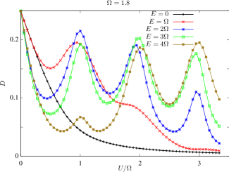
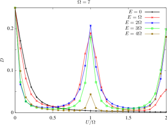
Figure 1: Double occupancy for the Falicov-Kimball model with ac-driven kinetic energy.

IV.1.2 Resonance and Fermi’s golden rule

In Fig. 2, we show (near-) resonant behavior of an ac-driven Falicov-Kimball model for values of $U$ close to $\Omega$ or $2\Omega$. The fraction of atoms in the higher Mott band $n_{\mathrm{up}}$, and the double occupancy $D$ are different from their equilibrium values when the driving amplitude $E$ is finite. We observe that $W=I$ in the full parameter range which we have explored. This implies that the system reaches the NESS. We clearly observe that $n_{\mathrm{up}}$, $D$, $W$ and $I$ have similar behavior as a function of $\frac{E}{\Omega}$, which can be understood as follows. In the strongly correlated regime, if atoms are excited to the higher Mott band, the double occupancy will increase, since most sites are singly occupied. Correspondingly, this means that the system absorbs energy from the driving fields. To keep it in the NESS, more energy should therefore be dissipated to the bath.

In the upper panel of Fig. 2, for $U$ close to $\Omega$, we observe that the behavior of these observables is qualitatively similar to $\left|\mathcal{J}_{1}\left(\frac{E}{\Omega}\right)\right|$, while in the lower panel, for $U$ close to $2\Omega$, it is similar to $\left|\mathcal{J}_{2}\left(\frac{E}{\Omega}\right)\right|$. It can be qualitatively described by Fermi’s golden rule. In the strongly correlated regime, the kinetic part can be treated as a perturbation relative to the interaction term. The transition amplitude between initial state $\left|I\right\rangle$ and final state $\left|F\right\rangle$ is Shirley (1965); Bilitewski and Cooper (2015)

$$A\left(I\rightarrow F,t\right)=\frac{-\mathrm{i}}{\hbar}\int_{0}^{t}dt^{\prime}e^{-\mathrm{i}\left(\mathcal{E}_{I}-\mathcal{E}_{F}\right)t^{\prime}}\left\langle\phi_{F}\right|\tilde{H}_{kin}\left(t^{\prime}\right)\left|\phi_{I}\right\rangle$$

where the kinetic part is $\tilde{H}_{kin}\left(t\right)=\sum_{\bm{k}}\epsilon_{\bm{k}-\bm{A}\left(t\right)}c_{\bm{k}}^{\dagger}c_{\bm{k}}$ with $\epsilon_{\bm{k}-\bm{A}\left(t\right)}=\epsilon_{\bm{k}}\cos\left(\frac{E}{\Omega}\sin\left(\Omega t\right)\right)+\bar{\epsilon}_{\bm{k}}\sin\left(\frac{E}{\Omega}\sin\left(\Omega t\right)\right)$, and where $\epsilon_{\bm{k}}=-2J\sum_{i=1}^{d}\cos k_{i}$ and $\bar{\epsilon}_{\bm{k}}=-2J\sum_{i=1}^{d}\sin k_{i}$. The transition probability $\gamma_{I\rightarrow F}=\lim_{t\rightarrow\infty}\frac{\left|A\left(I\rightarrow F,t\right)\right|^{2}}{t}$ takes the form

$$\gamma_{I\rightarrow F} =\sum_{\bm{k},\bm{k}^{\prime}}n_{\bm{k}}^{FI}n_{\bm{k}^{\prime}}^{IF}$$

$$\times \biggl{(}\epsilon_{\bm{k}}\epsilon_{\bm{k}^{\prime}}\sum_{l=even}\delta\left(\mathcal{E}_{I}-\mathcal{E}_{F}+l\Omega\right)\left|\mathcal{J}_{l}\left(z\right)\right|^{2}$$

$$+ \bar{\epsilon}_{\bm{k}}\bar{\epsilon}_{\bm{k}^{\prime}}\sum_{l=odd}\delta\left(\mathcal{E}_{I}-\mathcal{E}_{F}+l\Omega\right)\left|\mathcal{J}_{l}\left(z\right)\right|^{2}\biggr{)}$$ (11)

with $n_{\bm{k}}^{IF}=\left\langle I\right|c_{\bm{k}}^{\dagger}c_{\bm{k}}\left|F\right\rangle$ and $z=\frac{E}{\Omega}$. In the strongly correlated regime of an ac-driven Falicov-Kimball model, $\mathcal{E}_{\mathrm{I}}$ and $\mathcal{E}_{\mathrm{F}}$ are corresponding to the lower and upper Mott bands. From Eq. (11) we conclude that in an insulating state a $n\Omega$ ($n\geq 1$) resonance would be qualitatively described by $\left|\mathcal{J}_{n}\left(\frac{E}{\Omega}\right)\right|$.

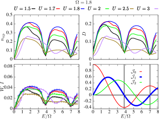
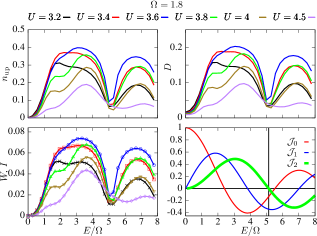
Figure 2: For the Falicov-Kimball model with ac-driven kinetic energy, we show the fraction of atoms excited to the upper band $n_{\mathrm{up}}$, double occupancy $D$, work $W$ (dots), energy dissipation $I$ (lines) and Bessel function of the first kind $\mathcal{J}_{l}\left(\frac{E}{\Omega}\right)$. At the one-photon resonance (upper panel), the oscillation is qualitatively described by $\left|\mathcal{J}_{1}\left(\frac{E}{\Omega}\right)\right|$, while the oscillation at the two-photon resonance qualitatively coincides with $\left|\mathcal{J}_{2}\left(\frac{E}{\Omega}\right)\right|$.

Alternatively, we can study the driven, strongly correlated regime using the Schrieffer-Wolff transformation Bukov et al. (2015, 2016). With a further rotation $V^{\prime}\left(t\right)=\exp\left[-\mathrm{i}Ut\sum_{i}c_{i}^{\dagger}c_{i}f_{i}^{\dagger}f_{i}\right]$ of the Hamiltonian $H=\tilde{H}_{kin}+H_{int}$, we have $\tilde{H}^{rot}=-J\sum_{l}\sum_{\left\langle ij\right\rangle}\mathcal{J}_{l}\left(z_{ij}\right)e^{\mathrm{i}l\Omega t+\mathrm{i}Ut\left(n_{fi}-n_{fj}\right)}c_{i}^{\dagger}c_{j}$. For the resonant case where $U=m\Omega$ with integer $m$, we have the effective Hamiltonian from the high-frequency expansion Bukov et al. (2016),

$$H_{eff}^{\left(0\right)}=-J\sum_{\left\langle ij\right\rangle}\left(\mathcal{J}_{0}\left(z_{ij}\right)\hat{g}_{f,ij}+\mathcal{J}_{m}\left(z_{ij}\right)\hat{h}_{f,ij}\right)c_{i}^{\dagger}c_{j}$$ (12)

where $z_{ij}=\frac{\bm{E}\cdot\left(\bm{R}_{i}-\bm{R}_{j}\right)}{\Omega}$ is limited to nearest neighbors, $\hat{g}_{f,ij}=\left(1-n_{fi}\right)\left(1-n_{fj}\right)+n_{fi}n_{fj}$ and $\hat{h}_{f,ij}=(-1)^{m}n_{fi}\left(1-n_{fj}\right)+\left(1-n_{fi}\right)n_{fj}$ with $n_{fi\left(j\right)}=f_{i\left(j\right)}^{\dagger}f_{i\left(j\right)}$. In Eq. (12), clearly the second term is introduced due to the resonance. We observe that with the same amplitude $\mathcal{J}_{m}\left(z_{ij}\right)$ the correlated hopping $c_{i}^{\dagger}c_{j}n_{fi}\left(1-n_{fj}\right)$ creates a double occupancy on site $i$, and that $c_{i}^{\dagger}c_{j}\left(1-n_{fi}\right)n_{fj}$ destroys a double occupancy. This explains why in Fig. 2 the double occupancy tends to follow the Bessel functions. It is consistent with our understanding from Fermi’s golden rule.

In Ref. Jordens et al. (2008), the energy gap of the Mott insulator of a Fermi-Hubbard model is determined by a distinct peak in the double occupancy when $U$ matches the modulation frequency. It can be understood as one-photon resonant tunneling, as we show in Figs. 1 and 2.

In the strongly correlated regime, an occupation of the upper Mott band dramatically changes the effective distribution $f_{\mathrm{eff}}\left(\omega^{\prime}\right)=\frac{N\left(\omega^{\prime}\right)}{A\left(\omega^{\prime}\right)}$ where $A\left(\omega^{\prime}\right)=-\frac{1}{\pi}\mathrm{Im}G^{R}_{nn}\left(\omega\right)$ and $N\left(\omega^{\prime}\right)=\frac{1}{2\pi}\mathrm{Im}G^{<}_{nn}\left(\omega\right)$. $\omega\in\left[-\frac{\Omega}{2},\frac{\Omega}{2}\right)$, and $\omega^{\prime}=\omega+n\Omega$. For the static case with half-filling, one has $N\left(\omega^{\prime}>0\right)=0$ while for the driven case $N\left(\omega^{\prime}>0\right)$ is finite, therefore $f_{\mathrm{eff}}\left(\omega^{\prime}\right)$ is very different from a Fermi-Dirac distribution. This is a characteristic of the NESS. For a static case, there are two Mott-bands separated by $U$. With driving turned on, there are quasi-energy bands with $n\Omega$ ($n\geq 1$ integer) energy difference from the bands of the static case. Excitations to the higher quasi-energy bands need assistance of a photon with frequency $n\Omega$. By occupation of the higher Mott band, the system absorbs energy from driving and dissipates it to the bath, so the energy dissipation rate $I$ is finite. From Eq. (9) we see that a nonzero $I$ implies a violation of the fluctuation-dissipation theorem Tsuji (2010).

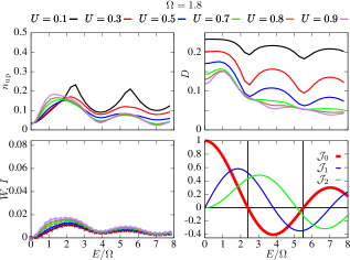
Figure 3: For the Falicov-Kimball model with ac-driven kinetic energy, the fraction of atoms excited to the upper band $n_{\mathrm{up}}$, double occupancy $D$, work $W$ (dots), energy dissipation $I$ (lines) and Bessel function of the first kind $\mathcal{J}_{l}\left(\frac{E}{\Omega}\right)$ are shown in the weakly interacting regime.

We also study the nonequilibrium behavior in the weakly-interacting regime. In Fig. 3, we find the double occupancy to be qualitatively controlled by $\left|\mathcal{J}_{0}\left(\frac{E}{\Omega}\right)\right|$ for weak $U$. It shows that the system is described by the effective Hamiltonian and in a (correlated) “metallic” state. A resonance is possible, as shown in the plot for $W$ and $I$ in Fig. 3, if the driving frequency can match the band-width. The minima of $W$ and $I$ are at the nodes of $\mathcal{J}_{1}\left(z\right)=0$ as before. This indicates that only the process of single-photon absorption occurs. However, the resonance is greatly suppressed.

To sum up, we have shown that in an ac-driven Falicov-Kimball model, driving frequency, driving amplitude and interaction strength are important parameters for controlling physical properties of the NESS. With a careful choice of these parameters, one can tune the NESS of the driven system very close to an effective equilibrium system. With good control of resonant tunneling, one can induce different populations of different Floquet bands and achieve the goal of “photo-doping”.

IV.2 Driven Interaction

In this section, we analyze the behavior of double occupancy due to periodic modulation of the interaction. We explain it by analytical calculation and using the information from spectral functions. We show that the NESS is reached within the framework of Floquet DMFT.

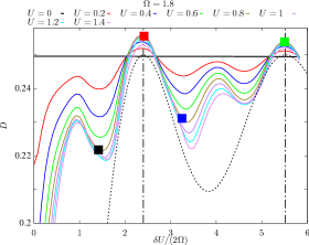
Figure 4: Double occupancy versus driving amplitude $\delta U$ for different values of $U$ and the driving frequency $\Omega$.

In Fig. 4, we plot the modulation of double occupancy $D$ versus driving amplitude for different interactions. We note the following observations. (i) When $U=0$, $D$ is not modulated by $\delta U$. This is due to the symmetry in the system Hamiltonian Liberto et al. (2014). (ii) When $U\neq 0$, we find that $D$ is modulated as a function of $\delta U$. (iii) Close to the position of the nodes ($\frac{\delta U}{2\Omega}=2.4,\;5.5,$ $\cdots$) of $\mathcal{J}_{0}\left(\frac{\delta U}{2\Omega}\right)$, we find that $D>\frac{1}{4}$ when $\delta U\gg U$. In the following, we explain (ii) and (iii) in order.

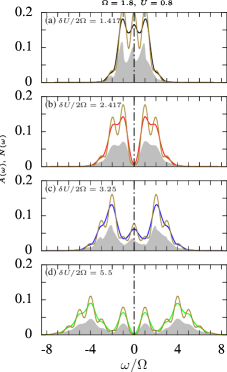
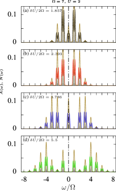
Figure 5: Spectral function $A\left(\omega\right)$ and occupied density of states $N\left(\omega\right)$ for points with same color indicated in Fig. 4. The olive lines are corresponding to $U=0$.

We first explain that the modulation of $D$ can be qualitatively described by $\mathcal{J}_{0}^{2}\left(\frac{\delta U}{2\Omega}\right)$. As shown in Sec. VI.2, the non-interacting retarded Floquet Green’s function for a system with time-periodically modulated interactions is

$$G_{mn}^{R\left(0\right)}\left(\omega\right) =\sum_{l}\mathcal{J}_{l-m}\left(\frac{\delta U}{2\Omega}\right)\mathcal{J}_{l-n}\left(\frac{\delta U}{2\Omega}\right)$$

$$\times\left(-\mathrm{i}\sqrt{\pi}e^{-\xi_{l}^{2}}\mathrm{erfc}\left(-\mathrm{i}\xi_{l}\right)\right),$$ (13)

where $\xi_{l}=\omega+l\Omega+\frac{U}{2}+\mathrm{i}\Gamma$. One can therefore expect that the dependence of the diagonal elements of the interacting Green’s function $\hat{G}^{R}\left(\omega\right)$ on $\frac{\delta U}{2\Omega}$ are described by a function related to the Bessel function $\mathcal{J}_{l}\left(\frac{\delta U}{2\Omega}\right)$. One further obtains $\hat{G}^{<}\left(\omega\right)=(\hat{G}^{R}\left(-2i\Gamma\hat{\bm{F}}+\hat{\Sigma}_{lat}^{K}\right)\hat{G}^{A}-\hat{G}^{R}+\hat{G}^{A})/2$ where $F_{mn}=F\left(\omega+n\Omega\right)\delta_{mn}$. From the impurity solver, we have $w_{1}\hat{R}\left(\omega\right)=\hat{G}\left(\omega\right)-w_{0}\hat{\mathcal{G}}_{0}\left(\omega\right)$. Since the double occupancy is given by $D=w_{1}\sum_{m}\int_{0}^{\Omega}\frac{d\omega}{2\pi}\mathrm{Im}\left[R_{mm}^{<}\left(\omega\right)\right]$, we conclude that $D$ is modulated by a function related to the Bessel function. Based on this observation, we plot $g\left(\frac{\delta U}{2\Omega}\right)=-\frac{1}{4}\mathcal{J}_{0}^{2}\left(\frac{\delta U}{2\Omega}\right)+\frac{1}{4}$ (black dashed line) in Fig. 4. We find that for the case of high driving frequency $D$ is well consistent with $g\left(\frac{\delta U}{2\Omega}\right)$. It is not easy to find an analytical formula for the interacting case, because all quantities involved are matrices. We present in Fig. 5 spectral functions for points of same color indicated in Fig. 4. We see that the density of states (DOS) around $\omega=0$ is tiny when $\frac{\delta U}{2\Omega}\approx 2.4,\,5.5$ compared to other values, which indicates that the DOS at $\omega=0$ is modulated by $\mathcal{J}_{0}^{2}\left(\frac{\delta U}{2\Omega}\right)$. A change in double occupancy $D$ involves excitations over the Fermi level at $\omega=0$. The small value of the DOS at $\omega=0$ makes high-order excitations very difficult because they require intermediate states close to $\omega=0$. Note that for this reason the gap around $\omega=0$ has approximately the width $2\Omega$ (see Fig. 5). This is the reason why $D$ can be affected by a modulation of the DOS around $\omega=0$.

We now explain why $D>\frac{1}{4}$ close to the nodes of $\mathcal{J}_{0}\left(\frac{\delta U}{2\Omega}\right)$ when $\delta U\gg U$. Using nonequilibrium DMFT, it has been found that $D\left(t\right)>\frac{1}{4}$ in a transient dynamics of a (driven) Hubbard model because of band flipping Tsuji et al. (2011, 2012), or a favoring of holon-doublon process due to dynamical localization Mendoza-Arenas et al. (2017). In our case, the situation is different because our system is driven in a different way, and we focus on the final NESS. For $\Omega=7$ and $U=2$ in Fig. 4, we look at the change of $D$ with increasing driving amplitude. For finite $U$, $D$ is small when $\delta U=0$. It is greatly enhanced because of photon-assisted tunneling with increasing $\delta U$. $D$ saturates close to the $\frac{\delta U}{2\Omega}\approx 2.4$, i.e. at the first node of $\mathcal{J}_{0}\left(\frac{\delta U}{2\Omega}\right)=0$, where the opening of a gap of the order of $2\Omega$ makes photon-assisted tunneling difficult (see Fig. 5). For $\Omega=1.8$, the change of $D$ is more complex because high-order processes are involved. Therefore, the role of photon-assisted tunneling is very important for the enhancement of $D$. At the nodes of $\mathcal{J}_{0}\left(\frac{\delta U}{2\Omega}\right)=0$, photon-assisted tunneling is possible to favor $D>\frac{1}{4}$ when $U$ is finite. A finite $U$ has two effects: it makes creation of doublon difficult, and it increases the band width to facilitate photon assisted tunneling over $2\Omega$ gap, which will further increase $D$. Figure 5 shows that the band width is enhanced by finite $U$ compared to the case $U=0$ (see olive lines in Fig. 5). Our calculation shows that the second effect dominates in the regime $\delta U\gg U,\Omega$.

In Fig. 6, the double occupancy is shown for different driving amplitudes and we see that the system is in the non-equilibrium state. (i) Compared to the non-driven case, the double occupancy $D$ is dramatically changed. For this high driving frequency ($\Omega=7$), we can see clear resonance peaks when $U=n\Omega$. As we have shown for the case of a driven kinetic energy, a well-defined resonant peak is corresponding to two well-separated Mott bands. (ii) For high-driving frequency and $\delta U=33.6$, i.e., $\frac{\delta U}{2\Omega}=2.4$, $D$ is close to 0.25. This is a reflection of the behavior of the double occupancy around the nodes of $\mathcal{J}_{0}\left(\frac{\delta U}{2\Omega}\right)$, which we observed in Fig. 4. It will not change dramatically until $U$ becomes the dominant energy scale.

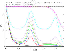
Figure 6: Double occupancy versus $U$ for different driving amplitudes with driving frequency $\Omega=7$.

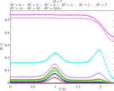
Figure 7: Work done by the driving field $W$ (dots), and energy dissipation to the bath $I$ (lines) as a function of $U$ for different driving amplitudes with driving frequency $\Omega=7$.

Finally, in Fig. 7, we clearly show that $W=I$ for the parameters in Fig. 6, which indicates that the NESS is reached. The work $W$ is defined as in Eq. (10). When the driving amplitude $\delta U=0$, there is no energy dissipation to the bath. When $U\neq n\Omega$, no resonant tunneling is possible and the dissipation is suppressed to relatively small values compared with those of resonant cases. This provides important information about parameter regions where the NESS is close to an equilibrium state.

To sum up, for time-periodically driven interactions, we show that relevant physical quantities are dramatically changed compared to the non-driven case. We find that the double occupancy is modulated as $\mathcal{J}_{0}^{2}\left(\frac{\delta U}{2\Omega}\right)$, and that it can exceed the value $\frac{1}{4}$ close to nodes of $\mathcal{J}_{0}\left(\frac{\delta U}{2\Omega}\right)$ when $\delta U\gg U$. We furthermore show that the NESS is reached throughout the parameter region which we have explored.

V Conclusions

In conclusion, we have systematically studied the NESS in a driven Falicov-Kimball model, with driven kinetic energy or driven interaction. (i) For an ac-driven kinetic energy, we show that the relevant physical quantities in the strongly correlated regime around the resonance can be qualitatively described by Bessel functions. We explain this phenomenon by Fermi’s golden rule, and by the Schrieffer-Wolff transformation of the driven Hamiltonian. These two understandings are consistent. Resonant tunneling is an efficient way to control the occupancy of Floquet bands and it can be used to achieve “photo-doping”. (ii) For driven interactions, we find that the double occupancy is dramatically modulated as a function of the driving amplitude. We find that close to the nodes of $\mathcal{J}_{0}\left(\frac{\delta U}{2\Omega}\right)$ the double occupancy can be larger than $\frac{1}{4}$ when $\delta U\gg U$, and we argue that this can be understood by taking into account the special role played by the DOS close to $\omega=0$, as well as the role of a small finite positive $U$. We demonstrate that the NESS is reached in both cases i) and ii).

In the future, we will investigate systems with double modulation, i.e. with simultaneously driven kinetic energy and driven interaction. As shown in Refs. Greschner et al. (2014a, b), one-dimensional strongly correlated systems with double modulation can have exotic and interesting physics. This will motivate studies of high-dimensional systems with double modulation using the non-perturbative method of Floquet DMFT.

VI Appendix

VI.1 Impurity solver for the Falicov-Kimball model with driven interactions

We derive the impurity solver for the Falicov-Kimball model with driven interactions. In the time domain, the impurity solver for the Falicov-Kimball model can be written as Aoki et al. (2014)

$$G\left(t,t^{\prime}\right)=w_{0}Q\left(t,t^{\prime}\right)+w_{1}R\left(t,t^{\prime}\right)$$ (14)

where $Q\left(t,t^{\prime}\right)$ and $R\left(t,t^{\prime}\right)$ are defined by the following equations,

$$\left[\mathrm{i}\partial_{t}+\mu\right]Q\left(t,t^{\prime}\right)-\left(\Delta\ast Q\right)\left(t,t^{\prime}\right)= \delta_{\mathcal{C}}\left(t,t^{\prime}\right),$$ (15)

$$\left[\mathrm{i}\partial_{t}+\mu-U\left(t\right)\right]R\left(t,t^{\prime}\right)-\left(\Delta\ast R\right)\left(t,t^{\prime}\right)= \delta_{\mathcal{C}}\left(t,t^{\prime}\right)$$ (16)

where $\left(A\ast B\right)\left(t,t^{\prime}\right)=\int_{\mathcal{C}}d\bar{t}A\left(t,\bar{t}\right)B\left(\bar{t},t^{\prime}\right)$. $\Delta\left(t,t^{\prime}\right)$ is the hybridization to a fictitious bath. Note all the Green’s function are defined on the Keldysh contour. We use Eq. (16) as an example to explain how to go to Floquet space. Firstly, we write all functions explicitly on the two Keldysh branches:

$$\left(\Lambda\ast R\right)\left(t,t^{\prime}\right)-\left(\Delta\ast R\right)\left(t,t^{\prime}\right)=\delta_{\mathcal{C}}\left(t,t^{\prime}\right)$$ (17)

where $\Lambda\left(t,\bar{t}\right)=\left(\mathrm{i}\partial_{t}+\mu-U\left(t\right)\right)\left(\begin{array}[]{cc}\delta_{11}\left(t,\bar{t}\right)\\ &\delta_{22}\left(t,\bar{t}\right)\end{array}\right)$. Then we go to the real axis Rammer (2007),

$$\left(\tau_{3}\Lambda\ast\tau_{3}R\right)\left(t,t^{\prime}\right)-\left(\tau_{3}\Delta\ast\tau_{3}R\right)\left(t,t^{\prime}\right)=\tau_{3}\delta\left(t,t^{\prime}\right).$$ (18)

With the Larkin-Ovchinikov transformation Aoki et al. (2014), we have

$$\left(\hat{\Lambda}\ast\hat{R}\right)\left(t,t^{\prime}\right)-\left(\hat{\Delta}\ast\hat{R}\right)\left(t,t^{\prime}\right)=\hat{\delta}\left(t,t^{\prime}\right)$$ (19)

where we should note that $\hat{\Lambda}\left(t,\bar{t}\right)$ and $\hat{\delta}\left(t,\bar{t}\right)$ are diagonal. The same procedure can be applied to Eq. (15). We can transform these equations to the frequency domain

$$\hat{G}\left(\omega\right)= w_{0}\hat{Q}\left(\omega\right)+w_{1}\hat{R}\left(\omega\right),$$ (20)

$$\hat{Q}_{mn}^{-1}\left(\omega\right)= \left(\omega+\mu+n\Omega\right)\delta_{mn}-\Delta_{mn},$$ (21)

$$\hat{R}_{mn}^{-1}\left(\omega\right)= \left(\omega+\mu+n\Omega\right)\delta_{mn}-U_{mn}-\Delta_{mn}.$$ (22)

These equations can be compactly written as

$$\hat{G}\left(\omega\right)=w_{0}\hat{\mathcal{G}}_{0}\left(\omega\right)+w_{1}\left(\hat{\mathcal{G}}_{0}^{-1}\left(\omega\right)-\hat{U}\left(\omega\right)\right)^{-1}$$ (23)

where $\hat{U}\left(\omega\right)=\left(\begin{array}[]{cc}\left(U_{mn}\right)&0\\ 0&\left(U_{mn}\right)\end{array}\right)$ with $\left(U_{mn}\right)$ a matrix consisting of elements $U_{mn}$. Equation (23) also applies if $U\left(t\right)$ is time-dependent.

VI.2 Non-interacting retarded Floquet Green’s function for modulated interactions

We write the Hamiltonian by explicitly including the chemical potential $\mu$

$$H_{s}=-J\sum_{\left\langle ij\right\rangle}c_{i}^{\dagger}c_{j}-\mu\sum_{i}c_{i}^{\dagger}c_{i}+\left(U+\delta U\cos\left(\Omega t\right)\right)\sum_{i}c_{i}^{\dagger}c_{i}f_{i}^{\dagger}f_{i}.$$ (24)

Imposing particle-hole symmetry at all time $t$, we find

$$\mu=\frac{1}{2}\left(U+\delta U\cos\left(\Omega t\right)\right).$$ (25)

One can transform the kinetic part to momentum space

$$H_{s}=-J\sum_{\bm{k}}\epsilon_{\bm{k}}\left(t\right)c_{\bm{k}}^{\dagger}c_{\bm{k}}+\left(U+\delta U\cos\left(\Omega t\right)\right)\sum_{i}c_{i}^{\dagger}c_{i}f_{i}^{\dagger}f_{i}$$ (26)

where $\epsilon_{\bm{k}}\left(t\right)=-2J\sum_{\alpha=1}^{d}\cos\left(k_{\alpha}\right)-\frac{1}{2}\left(U+\delta U\cos\left(\Omega t\right)\right)$. It has been shown Tsuji et al. (2008); Frank (2013); Aoki et al. (2014) that for a driven system the non-interacting retarded Green’s function can be expressed as

$$G_{\bm{k}}^{R0}\left(\omega\right)=\Lambda_{\bm{k}}\cdot\left[Q_{\bm{k}}^{-1}\left(\omega\right)+\mathrm{i}\Gamma\right]^{-1}\cdot\Lambda_{\bm{k}}^{\dagger}$$ (27)

where the term $\mathrm{i}\Gamma$ arises from the bath and

$$\left(\Lambda_{\bm{k}}\right)_{mn} =\int_{-\pi}^{\pi}\frac{dx}{2\pi}e^{\mathrm{i}\left(m-n\right)x}$$

$$\times\exp\left(-\frac{\mathrm{i}}{\Omega}\int_{0}^{x}dz\left[\epsilon_{\bm{k}}\left(\frac{z}{\Omega}\right)-\left(\epsilon_{\bm{k}}\right)_{0}\right]\right)$$

and $\left(Q_{\bm{k}}\right)_{mn}\left(\omega\right)=\frac{1}{\omega+n\Omega+\frac{U}{2}-\left(\epsilon_{\bm{k}}\right)_{0}+\mathrm{i}\eta}\delta_{mn}$. One obtains

$$G_{\bm{k}mn}^{R\left(0\right)}\left(\omega\right) =\sum_{l}\mathcal{J}_{l-m}\left(\frac{\delta U}{2\Omega}\right)\mathcal{J}_{l-n}\left(\frac{\delta U}{2\Omega}\right)$$ (28)

$$\times\frac{1}{\omega+l\Omega+\frac{U}{2}-\epsilon_{\bm{k}}+\mathrm{i}\Gamma}.$$ (29)

We next perform the integral over $\epsilon_{\bm{k}}$ for a Gaussian DOS Georges et al. (1996), which leads to

$$G_{mn}^{R\left(0\right)}\left(\omega\right) =\sum_{l}\mathcal{J}_{l-m}\left(\frac{\delta U}{2\Omega}\right)\mathcal{J}_{l-n}\left(\frac{\delta U}{2\Omega}\right)$$ (30)

$$\times\left(-\mathrm{i}\sqrt{\pi}e^{-\xi_{l}^{2}}\mathrm{erfc}\left(-i\xi_{l}\right)\right)$$ (31)

where $\xi_{l}=\omega+l\Omega+\frac{U}{2}+\mathrm{i}\Gamma$ and $\mathrm{erfc}\left(z\right)\equiv\frac{2}{\sqrt{\pi}}\int_{z}^{\infty}e^{-t^{2}}dt$.

References

- Aidelsburger et al. (2013) M. Aidelsburger, M. Atala, M. Lohse, J. T. Barreiro, B. Paredes, and I. Bloch, Phys. Rev. Lett. 111, 185301 (2013).
- Miyake et al. (2013) H. Miyake, G. A. Siviloglou, C. J. Kennedy, W. C. Burton, and W. Ketterle, Phys. Rev. Lett. 111, 185302 (2013).
- Jotzu et al. (2014) G. Jotzu, M. Messer, R. Desbuquois, M. Lebrat, T. Uehlinger, D. Greif, and T. Esslinger, Nature 515, 237 (2014).
- Jotzu et al. (2015) G. Jotzu, M. Messer, F. Görg, D. Greif, R. Desbuquois, and T. Esslinger, Phys. Rev. Lett. 115, 073002 (2015).
- D’Alessio and Rigol (2014) L. D’Alessio and M. Rigol, Phys. Rev. X 4, 041048 (2014); A. Lazarides, A. Das, and R. Moessner, Phys. Rev. E 90, 012110 (2014).
- Kuwahara et al. (2016) T. Kuwahara, T. Mori, and K. Saito, Ann. Phys. 367, 96 (2016).
- Abanin et al. (2015) D. A. Abanin, W. De Roeck, and F. m. c. Huveneers, Phys. Rev. Lett. 115, 256803 (2015).
- Bukov et al. (2015) M. Bukov, L. D’Alessio, and A. Polkovnikov, Adv. Phys. 64, 139 (2015).
- Tsuji et al. (2009) N. Tsuji, T. Oka, and H. Aoki, Phys. Rev. Lett. 103, 047403 (2009).
- Vorberg et al. (2013) D. Vorberg, W. Wustmann, R. Ketzmerick, and A. Eckardt, Phys. Rev. Lett. 111, 240405 (2013).
- Seetharam et al. (2015) K. I. Seetharam, C.-E. Bardyn, N. H. Lindner, M. S. Rudner, and G. Refael, Phys. Rev. X 5, 041050 (2015).
- Iwai et al. (2003) S. Iwai, M. Ono, A. Maeda, H. Matsuzaki, H. Kishida, H. Okamoto, and Y. Tokura, Phys. Rev. Lett. 91, 057401 (2003).
- Eckardt (2017) A. Eckardt, Rev. Mod. Phys. 89, 011004 (2017).
- Jaksch and Zoller (2003) D. Jaksch and P. Zoller, New J. Phys. 5, 56 (2003).
- Struck et al. (2011) J. Struck, C. Ölschläger, R. Le Targat, P. Soltan-Panahi, A. Eckardt, M. Lewenstein, P. Windpassinger, and K. Sengstock, Science 333, 996 (2011).
- Fläschner et al. (2016) N. Fläschner, B. S. Rem, M. Tarnowski, D. Vogel, D. S. Lühmann, K. Sengstock, and C. Weitenberg, Science 352, 1091 (2016).
- Desbuquois et al. (2017) R. Desbuquois, M. Messer, F. Görg, K. Sandholzer, G. Jotzu, and T. Esslinger, Phys. Rev. A 96, 053602 (2017).
- Görg et al. (2018) F. Görg, M. Messer, K. Sandholzer, G. Jotzu, R. Desbuquois, and T. Esslinger, Nature 553, 481 EP (2018).
- Kevrekidis et al. (2003) P. G. Kevrekidis, G. Theocharis, D. J. Frantzeskakis, and B. A. Malomed, Phys. Rev. Lett. 90, 230401 (2003).
- Abdullaev et al. (2003) F. K. Abdullaev, E. N. Tsoy, B. A. Malomed, and R. A. Kraenkel, Phys. Rev. A 68, 053606 (2003).
- Gong et al. (2009) J. Gong, L. Morales-Molina, and P. Hänggi, Phys. Rev. Lett. 103, 133002 (2009).
- Dirks et al. (2015) A. Dirks, K. Mikelsons, H. R. Krishnamurthy, and J. K. Freericks, Phys. Rev. A 92, 053612 (2015).
- Meinert et al. (2016) F. Meinert, M. J. Mark, K. Lauber, A. J. Daley, and H.-C. Nägerl, Phys. Rev. Lett. 116, 205301 (2016).
- Rapp et al. (2012) A. Rapp, X. Deng, and L. Santos, Phys. Rev. Lett. 109, 203005 (2012).
- Greschner et al. (2014a) S. Greschner, L. Santos, and D. Poletti, Phys. Rev. Lett. 113, 183002 (2014a).
- Greschner et al. (2014b) S. Greschner, G. Sun, D. Poletti, and L. Santos, Phys. Rev. Lett. 113, 215303 (2014b).
- Eckstein and Kollar (2008) M. Eckstein and M. Kollar, Phys. Rev. Lett. 100, 120404 (2008).
- Kollar et al. (2011) M. Kollar, F. A. Wolf, and M. Eckstein, Phys. Rev. B 84, 054304 (2011).
- Tsuji et al. (2008) N. Tsuji, T. Oka, and H. Aoki, Phys. Rev. B 78, 235124 (2008).
- Aoki et al. (2014) H. Aoki, N. Tsuji, M. Eckstein, M. Kollar, T. Oka, and P. Werner, Rev. Mod. Phys. 86, 779 (2014).
- Herrmann et al. (2016) A. J. Herrmann, N. Tsuji, M. Eckstein, and P. Werner, Phys. Rev. B 94, 245114 (2016).
- Freericks et al. (2006) J. K. Freericks, V. M. Turkowski, and V. Zlatić, Phys. Rev. Lett. 97, 266408 (2006).
- Joura et al. (2008) A. V. Joura, J. K. Freericks, and T. Pruschke, Phys. Rev. Lett. 101, 196401 (2008).
- Freericks and Joura (2008) J. K. Freericks and A. V. Joura, “Nonequilibrium density of states and distribution functions for strongly correlated materials across the mott transition,” in Electron Transport in Nanosystems, edited by J. Bonča and S. Kruchinin (Springer Netherlands, Dordrecht, 2008) pp. 219–236.
- Tsuji et al. (2014) N. Tsuji, P. Barmettler, H. Aoki, and P. Werner, Phys. Rev. B 90, 075117 (2014).
- Shirley (1965) J. H. Shirley, Phys. Rev. 138, B979 (1965).
- Schrieffer and Wolff (1966) J. R. Schrieffer and P. A. Wolff, Phys. Rev. 149, 491 (1966).
- Bukov et al. (2016) M. Bukov, M. Kolodrubetz, and A. Polkovnikov, Phys. Rev. Lett. 116, 125301 (2016).
- Görg et al. (2017) F. Görg, M. Messer, K. Sandholzer, G. Jotzu, R. Desbuquois, and T. Esslinger, (2017), 1708.06751 .
- Stöferle et al. (2004) T. Stöferle, H. Moritz, C. Schori, M. Köhl, and T. Esslinger, Phys. Rev. Lett. 92, 130403 (2004).
- Jordens et al. (2008) R. Jordens, N. Strohmaier, K. Gunter, H. Moritz, and T. Esslinger, Nature 455, 204 (2008).
- Greif et al. (2011) D. Greif, L. Tarruell, T. Uehlinger, R. Jördens, and T. Esslinger, Phys. Rev. Lett. 106, 145302 (2011).
- Dirks et al. (2014) A. Dirks, K. Mikelsons, H. R. Krishnamurthy, and J. K. Freericks, Phys. Rev. A 89, 021602 (2014).
- Tsuji (2010) N. Tsuji, Theoretical Study of Nonequilibrium Correlated Fermions Driven by ac Fields, Ph.D. thesis, Department of Physics, University of Tokyo (2010).
- Georges et al. (1996) A. Georges, G. Kotliar, W. Krauth, and M. J. Rozenberg, Rev. Mod. Phys. 68, 13 (1996).
- Lee and Park (2014) W.-R. Lee and K. Park, Phys. Rev. B 89, 205126 (2014).
- Eckstein (2009) M. Eckstein, Nonequilibrium dynamical mean-field theory, Ph.D. thesis, University Augsburg (2009).
- Yonezawa and Morigaki (1973) F. Yonezawa and K. Morigaki, Progress of Theoretical Physics Supplement 53, 1 (1973).
- Elliott et al. (1974) R. J. Elliott, J. A. Krumhansl, and P. L. Leath, Rev. Mod. Phys. 46, 465 (1974).
- Brandt and Mielsch (1989) U. Brandt and C. Mielsch, Zeitschrift für Physik B Condensed Matter 75, 365 (1989).
- Bilitewski and Cooper (2015) T. Bilitewski and N. R. Cooper, Phys. Rev. A 91, 033601 (2015).
- Liberto et al. (2014) M. D. Liberto, C. E. Creffield, G. I. Japaridze, and C. M. Smith, Phys. Rev. A 89, 013624 (2014).
- Tsuji et al. (2011) N. Tsuji, T. Oka, P. Werner, and H. Aoki, Phys. Rev. Lett. 106, 236401 (2011).
- Tsuji et al. (2012) N. Tsuji, T. Oka, H. Aoki, and P. Werner, Phys. Rev. B 85, 155124 (2012).
- Mendoza-Arenas et al. (2017) J. J. Mendoza-Arenas, F. J. Gomez-Ruiz, M. Eckstein, D. Jaksch, and S. R. Clark, Ann. Phys. 529, 1700024 (2017).
- Rammer (2007) J. Rammer, Quantum Field Theory of Non-equilibrium States (Cambridge University Press, 2007).
- Frank (2013) R. Frank, New J. Phys. 15, 123030 (2013).