A parallel algorithm for Hamiltonian matrix construction in electron-molecule collision calculations: MPI-SCATCI

Abstract

Construction and diagonalization of the Hamiltonian matrix is the rate-limiting step in most low-energy electron – molecule collision calculations. Tennyson (J Phys B, 29 (1996) 1817) implemented a novel algorithm for Hamiltonian construction which took advantage of the structure of the wavefunction in such calculations. This algorithm is re-engineered to make use of modern computer architectures and the use of appropriate diagonalizers is considered. Test calculations demonstrate that significant speed-ups can be gained using multiple CPUs. This opens the way to calculations which consider higher collision energies, larger molecules and / or more target states. The methodology, which is implemented as part of the UK molecular R-matrix codes (UKRMol and UKRMol+) can also be used for studies of bound molecular Rydberg states, photoionisation and positron-molecule collisions.

1 Introduction

Modelling low-energy electron-molecule scattering systems is vital to the understanding of a range of physical processes in fields such as plasma physics [1], astrophysics [2], cell and DNA damage [3]. There are a number of codes available for performing ab initio calculations on such collisions. The most general of these rely on use of the so-called close-coupling expansion where the scattering wavefunction, $\Psi_{k}$, is represented, at least in the region of the molecular target, by:

$$\Psi_{k}={\cal{A}}\sum_{ijn}\phi_{in}(x_{1},x_{2},....x_{N})u_{ij}(x_{N+1})a_{injk}+\sum_{\ell}\chi_{\ell}(x_{1},x_{2},...x_{N+1})b_{\ell k}$$ (1)

where $\phi_{in}$ are the target wavefunctions and $u_{ij}$ are continuum orbitals. The index $i$ is the target symmetry, $j$ is the continuum orbital index and $n$ counts over target states belonging to symmetry $i$. $\cal{A}$ is the anti-symmetrization operator to ensure that the target times continuum wavefunction obeys the Pauli principle. The $\chi_{\ell}$ are short-range or $L^{2}$ functions where all electrons occupy target orbitals; $x_{p}$ represents the coordinates of electron $p$ where it is assumed that the target has $N$ electrons and hence the scattering system has $N+1$ electrons. Finally, $a_{injk}$ and $b_{lk}$ are the variational coefficients obtained by diagonalization of the Hamiltonian.

A variety of different models can be represented by this close-coupling expansion [4], including ones based on the use pseudo-states to augment expansion in physical target states. This approach is employed in the R-matrix with pseudo-states (RMPS) procedure [5, 6, 7]. In general, the target wave-function is expanded in configuration interaction (CI) form as a linear combination of configuration state functions (CSFs) $\eta$:

$$\phi_{in}=\sum_{m}c_{imn}\eta_{im}.$$ (2)

The Hamiltonian matrix derived from the use close-coupling expansion described above has a characteristic structure, see Fig. 1 below. In 1996, Tennyson [8] showed that it was possible to exploit this structure to greatly speed-up the construction of scattering Hamiltonians. His algorithm, as implemented in module SCATCI and which is discussed in detail below, has formed the backbone of various implementations of the UK Molecular R-matrix codes [9, 10, 11, 12, 13]. The algorithm used by SCATCI is extremely efficient leading it to be used for extensive close-coupling calculations on electron collisions N${}_{2}^{+}$ [14], SiN [15], CH₃CN [16], uracil [17, 18] pyramidine [19] and many others systems, as well as for studies of positron–molecule collisions [20, 21, 22].

Hamiltonian construction and diagonalization is usually the slowest step in the ab initio treatment of low-energy electron-molecule scattering. While diagonalization can usually spread over a number of cores, SCATCI is currently limited by its serial nature. This step in the calculation can become expensive if one or more of the following applies: (a) the use of an extensive list target states and/or pseudo-state; (b) large target CI expansions; (c) large continuum orbital basis sets. With modern calculations it is quite possible that all three of these criteria apply and it is quite easy to design desirable but intractable calculations for even diatomic targets [23]. The recent development of the B-spline based UKRMol+ code [13, 24], which extends both the range of energies and size of target that it is possible to treat, has only further exacerbated this situation.

It would therefore appear timely to revisit Tennyson’s Hamiltonian build algorithm. This algorithm was designed to run on serial computers and, given the prevalence of modern multi-core architectures, it is on a parallel implementation that we particularly focus. At the same time, it has been recognized that the structure of various the Hamiltonian matrices that can be generated using this algorithm lend themselves to different diagonalization procedures [25, 22]. These different diagonalization options are also integrate into a new MPI code, MPI-SCATCI. The next section specifies the formal aspects of the new code. Section 3 introduces the code itself, which is freely available from the ukrmol-in project in the CCPForge program depository, Section 4 gives some illustrative timings. Our conclusions and suggestions for future work are given in Section 5.

2 Theory

Using the close-coupling expansion in the form of Eq. (1) and the target CI expansion of Eq. (2) to build the final Hamiltonian matrix one needs, at least in principle, to evaluate many Hamiltonian matrix elements of the form

$$H_{imj,i^{\prime}m^{\prime}j^{\prime}}=\langle\eta_{im}u_{ij}|\hat{H}|\eta_{i^{\prime}m^{\prime}}u_{i^{\prime}j^{\prime}}\rangle$$ (3)

In practice the CSFs are expanded in terms of an orthogonal set of spin-orbitals which in turn are represented by atom and molecule centred functions of various types [26], which are discussed further below. However, we note that for accurate calculations, the target CI expansions can be very long and the the number of target states is usually significantly smaller than the number of target CSFs. To allow the identification of target states within the expansion, for example to correctly assign asymptotic channels, it is desirable to contract the matrix:

$$\tilde{H}_{inj,i^{\prime}n^{\prime}j^{\prime}}=\sum_{m,m^{\prime}}c_{imn}c_{i^{\prime}m^{\prime}n^{\prime}}H_{imj,i^{\prime}m^{\prime}j^{\prime}}$$ (4)

where $c_{imn}$ is the coefficient of the target CI expansion, see Eq. (2). The target-$L^{2}$ part of the calculation undergoes a similar contraction scheme:

$$\tilde{H}_{inj,l}=\sum_{m}c_{imn}H_{imj,l}.$$ (5)

These steps very significantly reduce the size of the Hamiltonian, hence the description contraction, and the majority of matrix elements retained are usually between the $L^{2}$ functions.

2.1 Symbolic evaluation, prototyping and expansion

Whilst the matrix itself is smaller, evaluating Eq. (4), in principle, requires the evaluation of all integrals in Eq. (3). SCATCI implements the algorithm of Tennyson [8] that avoids evaluating integrals and explicit computation of the un-contracted Hamiltonian. This is done through the manipulation of symbolic matrix elements [27] generated using prototype CSFs [28, 29]. This procedure exploits the structure of the scattering wavefunction, see Eq. (1), where a particular target wavefunction or CSF is multiplied by a (long) list of continuum functions.

The Hamiltonian construction is driven from a list of CSFs. The required integrals are identified by the application of Slater’s rules to give a list of symbolic matrix element. The published versions of the UKRMol/UKRMol+ codes are based on a traditional algorithm for Slater’s rules. Scemama and Giner [30] proposed an alternative algorithm that represents all possible spin orbitals that an electron can occupy as an array of 64-bit integers. Each integer can represent 64 spin orbitals and each set bit in the $n^{\rm th}$ position represents an electron occupying the $n^{\rm th}$ spin orbital. Determining the substitutions between two determinants can be easily computed by performing an exclusive-or (XOR) followed by a population count (popcnt). Their algorithm also determines the resultant phase from possible spin orbital reordering by computing the number of occupied orbitals between the differing orbitals using bit masks. A bug fix was applied to their optimized implementation that caused incorrect masks to be generated when orbital indices where of a multiple of 64, this fix has since been applied to the original authors source code. The majority of the computation relies mainly on hardware native instructions such as bit shifts, XOR and popcnt (AVX+ instruction set) making it extremely efficient and reducing overall Hamiltonian build times by factors of two to five. This algorithm is also independent of the number of electrons making it ideal for large polyatomic molecules. This efficient algorithm is the one used in MPI-SCATCI

To briefly summarize, the SCATCI procedure involves transforming the evaluation of both Hamiltonian into symbolic form. For Eq. (3) this is of the form:

$$H_{imj,i^{\prime}m^{\prime}j^{\prime}}=\sum_{\alpha}C^{\alpha}_{imj,i^{\prime}m^{\prime}j^{\prime}}X(I^{\alpha}_{imj,i^{\prime}m^{\prime}j^{\prime}})$$ (6)

Where $\alpha$ are the associated integral indices $I^{\alpha}$ and coefficients $C^{\alpha}$ generated for the matrix element and $X$ is the integral function. Within the UK molecule R-matrix codes, the indices are four 16-bit integers representing the associated orbitals in the integral packed into a 64-bit integer. As the configurations obey the Slater-Condon rules, there are a fixed number of one and two electron integrals that can be precomputed ahead of time. Therefore, $X$ is a function that maps the indices $I$ into a one and two-electron integral array and returns the appropriate integral value.

The contracted matrix can also be expressed similarly:

$$\tilde{H}_{inj,i^{\prime}n^{\prime}j^{\prime}}=\sum_{\beta}D^{\beta}_{inj,i^{\prime}n^{\prime}j^{\prime}}X(I^{\beta}_{ij,i^{\prime}j^{\prime}})$$ (7)

Whilst there are essentially no integral evaluations, large numbers of continuum orbitals and target configurations make this computationally undesirable. One way this is circumvented is to utilize symbolic prototyping. This methodology removes the need to explicitly evaluate matrix elements for each continuum orbital $j$ by instead evaluating the full Hamiltonian matrix elements for one or two prototype configurations corresponding to one or two $j$ and generating the full symbolic lists by manipulating the integral indices. This is the essence of Tennyson’s algorithm [8].

Transformation the full Hamiltonian matrix to the CI contracted one can be performed by contracting the minimal prototype symbolic elements of $H$. The prototype integral labels do not change but the associated coefficients do depending on the target symmetries and states:

$$D^{\beta}_{inj,i^{\prime}n^{\prime}j^{\prime}}=\sum_{m,m^{\prime}}c_{imn}c_{i^{\prime}m^{\prime}n^{\prime}}C^{\alpha}_{imj,i^{\prime}m^{\prime}j^{\prime}}$$ (8)

after which the labels are expanded into the full range of $j$. This means that the full Hamiltonian is never explicitly evaluated.

2.2 Matrix classes

The consequence of this contraction is that the matrix is now split into differing contraction classes based on the symmetry properties of the target states and the $L^{2}$ functions. Below is a summary of these contracted classes with Figure 1 illustrating them. Since the Hamiltonian is real symmetric, only the lower triangular portion is considered.

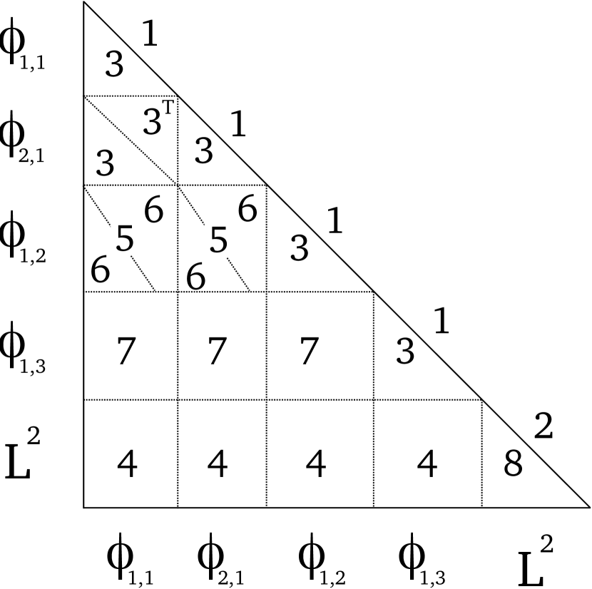
Figure 1: Class structure of the contracted Hamiltonian for a scattering calculation with three target symmetries. $\phi_{i,j}$ denotes a target state $i$ for a target symmetry $j$. Target symmetries 1 and 2 couple to the same continuum symmetry and symmetry 1 has two target states $\phi_{1,1}$ and $\phi_{2,1}$.

2.2.1 Classes 1 and 3

Classes 1 and 3 involve matrix elements between functions with the same target symmetry. Class 1 are the diagonal matrix elements involving a target state times a continuum orbital. These integrals can also occur in off-diagonal elements involving different states of the same symmetry. Class 3 are the off-diagonal elements involving different target states of a given symmetry; they have a symmetric block structure. The upper triangular block is the transpose of the lower triangular. The contraction is of the form:

$$\tilde{H}_{inj,in^{\prime}j^{\prime}}=\sum_{m,m^{\prime}}c_{imn}c_{imn^{\prime}}H_{imj,imj^{\prime}}+\sum_{m,m^{\prime}}(c_{imn}+c_{im^{\prime}n^{\prime}}+c_{im^{\prime}n}c_{imn^{\prime}})H_{imj,im^{\prime}j^{\prime}}$$ (9)

The symbols are then expanded for all target states and continuum orbitals of the target symmetry.

2.2.2 Classes 2 and 8

Classes 2 and 8 are the diagonal and off-diagonal matrix elements of the $L^{2}$ functions. These undergo no form of contraction and are instead evaluated explicitly. These are referred below to as ‘pure $L^{2}$’ elements.

2.2.3 Classes 5 and 6

These classes involve elements where the target symmetry differs but their coupled continuum symmetry is the same. Class 5 is the diagonal element of the local matrix block and class 6 is the off-diagonal element. The contraction scheme is of the form:

$$\tilde{H}_{inj,i^{\prime}n^{\prime}j^{\prime}}=\sum_{m,m^{\prime}}c_{imn}c_{i^{\prime}m^{\prime}n^{\prime}}H_{imj,i^{\prime}m^{\prime}j^{\prime}}$$ (10)

2.2.4 Class 7

This class involves matrix elements where both the target and continuum symmetry differs. The contraction is the same as Eq. (10) and is expanded across both target states and continuum orbitals of the target symmetries

2.2.5 Class 4

For matrix elements between continuum and $L^{2}$ functions the contraction is one-dimensional and is of the form given by Eq. (5).

2.2.6 Sparsity and diagonalization

For almost all classes, the matrix blocks are dense with the exception of the off-diagonal pure-$L^{2}$ class which is sparse. An example test case calculation of electron-H₂O [31] given in Figure 2 illustrates these properties. The nature of the matrix changes depending on the choice of CSF. For this test case, the matrix is considered dense due to the smaller number of $L^{2}$ functions, which encourages the usage of a dense diagonalizer such as LAPACK[32]. When dealing with large scattering systems of interest such as phosphoric acid, the number of $L^{2}$ functions can be several orders of magnitude larger than the size of the contracted part of the matrix. The matrix at this point becomes extremely sparse and may necessitate usage of a sparse diagonalizer such as ARPACK[33].

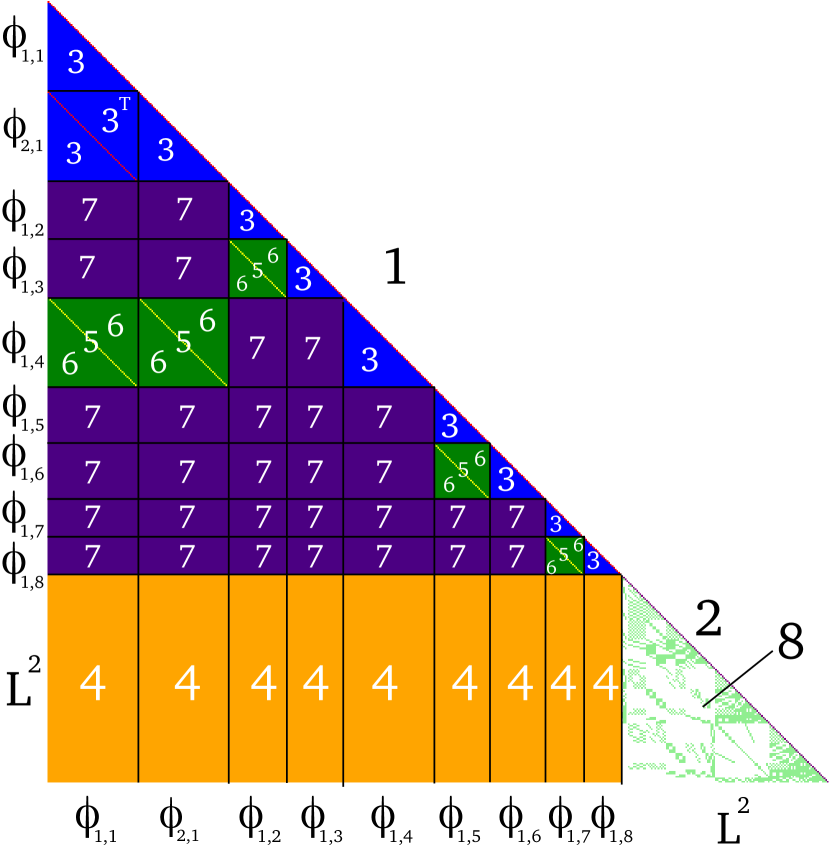
Figure 2: The lower-triangular Hamiltonian output for a test case for H₂O with 8 target symmetries and 4 continuum symmetries. Symmetry 1 has two target states. Target symmetries 1 and 4 both couple to the continuum symmetry 4, denoted by $(1,4)\rightarrow 4$, leading to the appearance of contraction classes 5 and 6 in the matrix blocks ($\phi_{1,4}$,$\phi_{1,1}$) and ($\phi_{1,4},\phi_{2,1}$). Other couplings include:  $(2,3)\rightarrow 3$, $(5,6)\rightarrow 2$, $(7,8)\rightarrow 1$. White colors represent zero values.

2.3 The UK-molecular R-matrix codes

The UK-molecular R-matrix suite, UKRMol [10], and its new enhanced version, UKRMol+ [13], are a set of modules and programs to fully solve the electron/positron-molecule scattering problem using the R-matrix methodology. The suite splits into two sets of codes: UKRMol-in which deals with the inner-region problem and UKRMol-out which deals with the outer region.

The codes use a a variety of methods to represent the target and continuum functions. The original code [9] only consider electron collisions with diatomic molecules; it was based on the use of Slater type orbitals (STOs) to represent the target wavefunction and suitably orthogonalised [34] numerical functions for the continuum. The original polyatomic code [35, 10] uses Gaussian type orbitals (GTOs) for both the target and the continuum functions. The new UKRMol+ [13] also uses GTOs to represent the target but uses a hybrid GTO – B-spline basis set for the continuum. One effect of this is that the continuum expansions can become significantly larger as the code allows treatment of more partial waves (higher $\ell$ values), larger R-matrix spheres and extensions to higher energies, all of which lead to an increase in the number of continuum functions.

A crucial module in both UKRMol and UKRMol+ is SCATCI [8]. SCATCI is a Fortran 77 code that deals with the building and diagonalization of the inner-region $N+1$ scattering Hamiltonian and is the last step before moving into the outer-region portion of the calculation.

3 MPI-SCATCI

MPI-SCATCI is a complete rewrite of SCATCI in Modern Fortran (2003) that uses MPI to perform both the N+1 Hamiltonian build and diagonalization. Its design is heavily based on an Object-Orientated Programming (OOP) paradigm to give the code a high degree of flexibility for further modification. Whilst previously integrating features such as a new integral format required a fair amount of modification to build subroutines, the OOP approach allows simply for the definition of a new Integral class with appropriate procedures that is then attached to the Hamiltonian at run time without touching the build code. Similar functionality also applies to the diagonalizers and as will be discussed later on in Section 3.2, gives MPI-SCATCI the ability to support almost any diagonalizer library and matrix format with little to no modification.

3.1 Build parallelization

There are three avenues for parallelisation of the scattering Hamiltonain: Across prototyping and contraction, across the expansion and across the L² functions. The choice is dependant on the type of matrix class being calculated. Regardless of which method is used, every process performs the same class and the same target symmetry for the contracted classes as it simplifies the distribution of work.

3.1.1 Classes 2 and 8

These pure-$L^{2}$ elements are the most straightforward to consider as no contraction is required. Each Slater-Condon calculation gives symbols for a single matrix element. MPI-SCATCI combines both classes into a single calculation and the nested loop over the lower triangular is collapsed into a single loop. This loop is evenly distributed across all MPI processes and computed independently with no need for any form of communication. Viewing the calculation as a whole (as seen in Figure 3), ’collectively’ all matrix elements have been calculated. This is the parallelisation that is also used in the construction of the target Hamiltonian whose solutions are required to give the target wavefunction coefficients, see Eq. (2), and associated energies, see below.

Figure 3: A visual representation of two processes evaluating the matrix elements of classes 2 and 8 in the scattering Hamiltonian

3.1.2 Classes 1, 3, 5, 6, 7

For pure continuum classes, there is a two step parallelization that occurs. Figure 4 visually describes this process. The first step consists of parallelizing the prototype and contraction stage. The loop across prototype CSFs are evenly distributed among MPI processes. This means each processor $p$ produces an incomplete list of contracted prototype symbols $\tilde{H}^{p}_{inj,i^{\prime}n^{\prime}j^{\prime}}$. At this point, a gather and reduce is performed on all $P$ processes in order to retrieve the complete set of contracted prototype symbols:

$$\tilde{H}_{inj,i^{\prime}n^{\prime}j^{\prime}}=\sum_{p}^{P}\tilde{H}^{p}_{inj,i^{\prime}n^{\prime}j^{\prime}}$$ (11)

Whilst this is a significant synchronization step, it is only performed

$$\frac{n_{t}(n_{t}+1)}{2}$$ (12)

times where $n_{t}$ is the number of target symmetries. This, in general, is small number of synchronization points as the number of target symmetries in a calculation is rarely larger than single digits.

The second step is the expansion of the prototype symbols. Very little work is actually done during the expansion as it only requires modifying the indices of the integral label for each continuum orbital. However, some systems have target symmetries that are coupled to thousands of continuum orbitals. Their prototypes require expanding for millions of matrix elements for the off-diagonal classes 3, 5, 6 and 7. Originally each process performed the full expansion on their incomplete symbols followed by a reduction to retrieve the full matrix element. This unfortunately became a significant bottleneck for continuum heavy systems and therefore necessitated the need for parallelizing the expansion process as well. The parallelization of the expansion is performed by evenly distributing processes across the $j,j^{\prime}$ expansion loop. Essentially, this step behaves similar to classes 2 and 8 and collectively the full matrix elements are computed. This two step approach benefits two types of problem sizes. For systems with a large number of prototype CSFs, the first step gives the greatest gain in performance. For systems with target symmetries that contain a huge number of continuum orbitals, the second stage provides the greatest benefit.

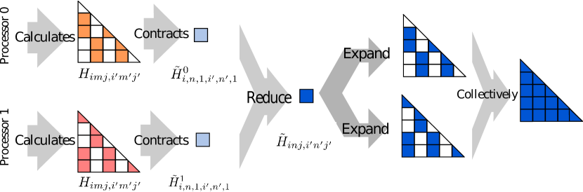
Figure 4: A visual representation of two processes evaluating the matrix elements of continuum only classes. The first stage involves computing and contracting the prototype elements into the first incomplete symbolic elements of the contracted matrix. The second stage is the all process reduction into the full symbolic prototype list. The last stage is the expansion across $j,j^{\prime}$ for each process. This means that both processes collectively have the full contracted matrix.

The original SCATCI had the option to remove all integrals involving only target orbitals from the matrix elements of classes 1, 3, 5, 6 and 7. These are replaced by adding the appropriate (precomputed) target energy along the diagonal. This approach has a number of advantages: it significantly reduces the number of integral evaluations and facilitates the manipulation of target energies, see Ref. [36] for example. In future we plan to use this facility, which is retained in MPI-SCATCI, to simplify the treatment heavy atoms via the use of effective core potentials.

As discussed by Orel et al. [37], there can be a technical issue with phases of the wavefunctions generated in a pure target calculation (Eq. (2)) and the scattering wavefunction (Eq. (1)) to do with order in which the electrons are treated in the CSFs. Ignoring this problem has in the past led to generation of incorrect results, see Gillan et al. [38]. SCATCI resolves this problem by using a phase mask which matches the phases between the two wavefunctions [39]. This is retained in MPI-SCATCI.

3.1.3 Class 4

Class 4 is the off-diagonal continuum-$L^{2}$ portion of the matrix. This presents a problem as it requires prototyping and expansion for each target symmetry and $L^{2}$ function. The number of $L^{2}$ functions in a typical calculation is significantly larger than size of the contracted continuum. This presents a problem with the two step procedure as each $L^{2}$ function for each symmetry would require a prototype synchronization step resulting in possibly millions in order to complete.

However we can exploit the fact that the prototyping, contraction and expansion are all one-dimensional loops as given by Eq. (5). This means that a class calculation for each $L^{2}$ function is significantly easier and faster to perform than any other contracted class. With this, the parallelization is instead performed across $\ell$ functions for a specific target symmetry independent of any other process and eliminating any costly synchronization. This is illustrated in Figure 5

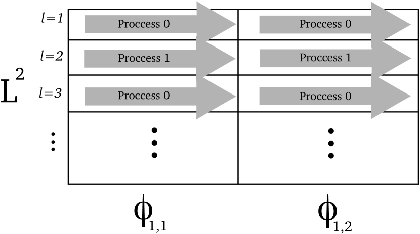
Figure 5: A visual representation of the class 4 prototyping and expansion of a single target symmetry block containing two states using two processes. The arrows represent the direction of generation of matrix elements. The processes are distributed in a round robin style across each $\ell$ function then prototype, contract and expand for all target states in the symmetry.

3.2 Matrix distribution

One of the key goals for the MPI code is to not only support the diagonalizer already included in the serial SCATCI code but also a wide range of MPI diagonalizers. Since often all eigenvectors are required, a dense diagonalizer such as SCALAPACK [40] is ideal for its efficient householder approach. However, for scattering Hamiltonians that have sizes in the order of millions, an iterative diagonalizer, such as the Scalable Library for Eigenvalue Problem Computations (SLEPc)[41], is more desirable as matrix sparsity can be exploited for storage and often these sizes arise in partitioned R-matrix problems that require only a small percentage of eigenvectors.

The Hamiltonian should therefore be built with regards to the final processor arrangement of the matrix elements. However both SCALAPACK and SLEPc have vastly different methods of storing the matrix. SCALAPACK uses a block-cyclic distribution and SLEPc uses a blocked row distribution. In addition, SLEPc requires the upper triangular matrix in C-style indexing. Therefore separate Hamiltonian builds would be required for each type of matrix distribution. This presents a huge cost in time to write, test and debug every Hamiltonian for every distribution.

3.2.1 Matrix formats

In MPI-SCATCI, an abstract BaseMatrix class is defined which provides the Hamiltonian a standard routine to store a matrix element. An inherited abstract DistributedMatrix class is also defined which will distribute the matrix elements in any format. It works by allowing the processes to touch every single matrix element at least once at some point during execution and by applying rules.

The rules are defined by a virtual boolean function. Each inherited matrix format must define this function in order to properly place matrix elements into the correct process. Two types of storage are defined, hot and cold storage. Hot storage is temporary storage for matrix elements that, after applying rules, do not belong to the computing process. This type of storage is the same for all distributed matrix class. Cold storage is the permanent storage of matrix elements that will eventually be used in diagonalization. Its representation depends on the format, for SCALAPACK it is the local matrix array, for SLEPc it is a Petsc Mat object. At some point during the build an update can be triggered. This update consists of rotating the hot storage in a ring like fashion across every process as illustrated in Figure 6 and applying the defined rules to each element for possible placement into cold storage. This means that communication through an interconnect only occurs with 2 of the processors in a node giving a communication overhead of the order $2(n-1)$ where $n$ is the number of nodes. Once each processes hot storage has completed a circuit, it is cleared and ready for usage again.

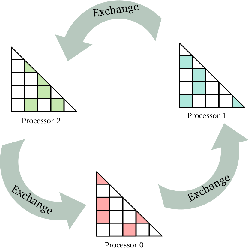
Figure 6: Ring rotation of the each processes hot storage

An update is triggered through two means: When memory has been exhausted and when the Hamiltonian build is completed. MPI-SCATCI tracks available free memory and when a process has exhausted all of its available memory, this signals all other processes to begin an update. This has the benefit in that when either given more RAM or more processes, the number of updates required in a run decreases. This is because we can either store more matrix elements or that we are storing less matrix elements per process. As will be discussed in Section 4 the update time remains essentially constant across processor counts.

This DistributedMatrix has proved beneficial as, barring initialization, requires only a single function definition to support the appropriate format without touching the Hamiltonian build. Currently, MPI-SCATCI has defined three types of distributed matrices:

• SCALAPACKMatrix

  • Stores local matrix in block cyclic distribution

  • Used by SCALAPACK diagonalizer

  • Distribution rule:

    • Call INFOG2L. If it belongs to me then store and return true otherwise false

• SLEPcMatrix

  • Stores in a PETSc Mat object in blocked row distribution

  • Used by SLEPc diagonalizer

  • Distribution rule:

    • Convert into upper triangular matrix and C index format

    • If it is within block row, store and return true otherwise false

• WriterMatrix

  • Writes matrix elements to file

  • Used by original SCATCI diagonalizers

  • Distribution rule:

    • If I am master process, store (and write) and return true, otherwise false

The SLEPcMatrix class presents another interesting feature, the rule function can also be used to preprocess a matrix element and in this case, convert into upper triangular and C-style indexing before storing. Additionally, PETSc matrix assembly time is non-existent as the elements are all in the correct process.

3.2.2 Diagonalization

The abstract Diagonalizer class provides a standard diagonalization routine that accepts a BaseMatrix as input. There is, however, no standard matrix element retrieval routine due to the vastly differing ways the matrix is stored (and sometimes not stored). Whilst it is technically valid to pass any BaseMatrix into any diagonalizer routine, it is up to the implementer to determine how to access the element for each format. The currently implemented diagonalizers perform a type check on the matrix pointer and either halts if it is not supported or calls the correct subroutine that typecasts back into its derived class. Whilst this seems to go against the OOP approach used in the rest of the code, the performance benefits are massive. For the SCALAPACK diagonalizer, the SCALAPACKMatrix provides the correct local array to immediately begin diagonalization and the same goes for the SLEPc diagonalizer and its corresponding matrix.

It is also worth noting that both SLEPc and SCALAPACK can be used in the same run. It is common for a run to use SLEPc to retrieve the target coefficients for the Hamiltonian build to then shift to SCALAPACK for the diagonalization of the scattering Hamiltonian. The diagonalizers currently supported by MPI-SCATCI are: LAPACK, Davidson [42], ARPACK, SCALAPACK and SLEPc and all can be mixed in the same run. Additionally, there is an experimental feature for non-MPI diagonalizers to utilize all threads in a node by sleeping other MPI processes whilst the master process performs OpenMP diagonalization. This is beneficial for the parallel MKL LAPACK as it is generally more efficient in a single node than SCALAPACK. However, this feature is unreliable as it is dependant on the non-polling barrier implementation of the MPI library and the pinning modes used.

3.3 Large Integrals

Under MPI, each process is given a private memory space. Taking an example 24-core node with 64 GB of memory and distributing evenly, this allows for a maximum of 2.5 GB per MPI process. Each process must store its own local copy of the CSFs, the local matrix and the integrals with this small amount of memory. The biggest cost comes from the integrals themselves. For instance, a the UKRMol phosphoric acid scattering calculation considered below requires 1.5 GB of memory to store the integrals leaving only 1 GB for everything else. This is a bigger issue with UKRMol+ calculations using B-splines. The integrals for the recent electron-beryllium mono-hydride (BeH) UKRMol+ calculation [24] require 3.0 GB, preventing them from being used as one of our example systems. Scattering calculations on larger systems such as uracil using B-splines may require tens of gigabytes of memory to store all of the integrals.

The fundamental issue is that the integral data is being repeated multiple times in each node as illustrated in Figure 7a. Naturally a method of distributing the integrals is needed and there are many to choose from.

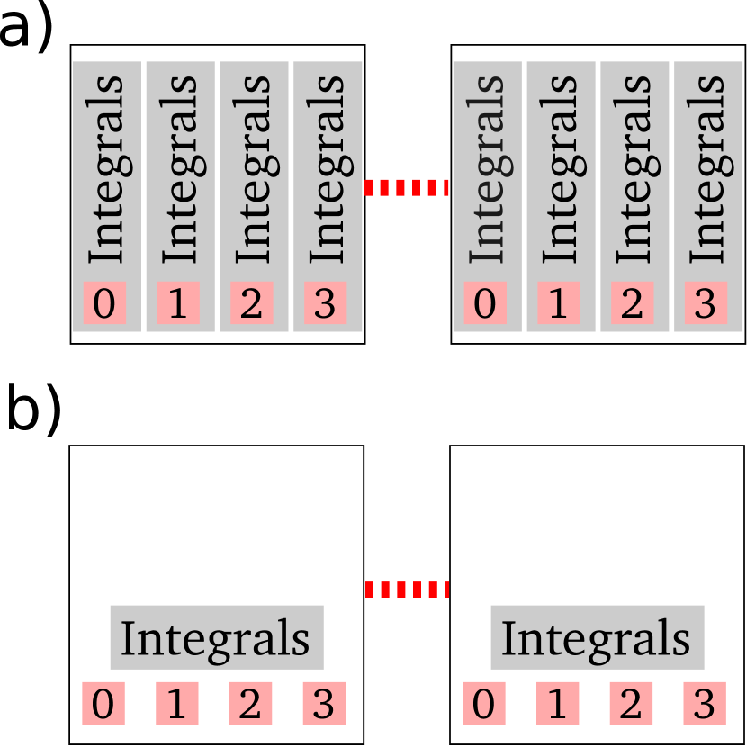
Figure 7: Two Memory layouts of the integrals for two four-core nodes with interconnect (red) between the two. a) The standard private memory layout under MPI and highlights the amount of repeated data on each compute node. b) MPI-3.0 Shared memory layout, Only a single instance of the integral is loaded for each node.

Firstly, an integral scatter method could be implemented where each process has a portion of the integrals and are then moved across when necessary. However it is difficult to predict which integrals are needed by which process and this is compounded by the fact that expansion of the prototype elements can introduce hundreds of differing integrals that are not present within the computing process. In a sense, at each integral evaluation it is likely that there will be a significant degree of communication which will kill performance, especially at higher process counts.

Another method would be to reduce the number of MPI processes in each node but to then restore parallel performance by utilizing OpenMP. A single occurrence of the integral could occur at each node giving us a large amount of memory to store integrals as well as minimizing the communication cost in synchronization as it will only occur at each node rather than each process. However, OpenMP 4.0 support of modern Fortran is still not mature enough and language features such as polymorphism are not fully supported resulting in crashes. Additionally some MPI diagonalizers are not hybrid OpenMP+MPI and therefore suffer in performance.

The method used by MPI-SCATCI utilizes a feature of the MPI-3.0 standard: Shared memory

3.3.1 Shared Memory

Shared memory is a feature which allows a portion of memory to be seen by a group of processes. This feature was actually present in some form with the MPI-2.0 standard through the use of windows but was in a sense a collective operation requiring many synchronizing ’epoch’ in order to get or put. Additionally it is not aware of the node-locality of certain processes and assumes remote memory access (RMA) at all times. The MPI-3.0 standard introduces a new communicator: MPI_COMM_TYPE_SHARED. this communicator groups process by which node they occur in. A shared window can be allocated that is node aware and removes the need for RMA, improving memory access times. Additionally there is no need for synchronization for any puts or gets but is still necessary to ensure no race conditions occur. However this is ideal as the integrals, once loaded, become read only eliminating any further fencing on gets. The elimination of fencing also prevents costly cache synchronization steps though there are still local cache misses due to the random access nature of the integrals. The simplicity of this usage is a significant advantage as the shared memory array behaves identically to a normal Fortran array once it has been set up. The memory layout of our integrals now reflects the illustration in Figure 7b and affords the code the ability to handle extremely large integrals that fit within the nodes total memory.

A new module was created in order to facilitate this functionality. It replaces the standard Fortran allocate function for arrays that we wish to share. For example, allocating an array for the one electron integrals:

⬇

allocate(one_e_int(num_one_e_int),stat=ifail)

Becomes this:

⬇

one_electron_window = mpi_memory_allocate_real(one_e_int,num_one_e_int)

If there is no available MPI-3.0 library, this will fallback into the standard Fortran allocate routine. The window variable is used both for determining if shared memory is being used and for deallocation. No other change in the integral routines is necessary. No change in performance has been observed between having a local private copy of the integrals and utilizing shared memory.

4 Performance

MPI-SCATCI has been successfully run and benchmarked on both University College London’s Grace@UCL supercomputing cluster and ARCHER, the UK National Supercomputer Service. Grace@UCL has 360 nodes each with 16 Intel Haswell cores and 64 GB of memory connected by non-blocking Intel Truescale Infiniband. ARCHER’s Cray XC30 nodes comprise of two 2.7 GHz, 12-core E5-2697 v2 CPUs with 32 GB each arranged in a non-uniform memory access (NUMA) configuration giving 24 cores and 64 GB total connected with Cray Aries interconnect. The benchmark runs all stored the scattering Hamiltonian on disk rather than in a format ready for diagonalization. This is to allow a better ’apples to apples’ comparison to the serial SCATCI code and the fact that we are not assessing the performance of the diagonalizers themselves. This will still test the matrix distribution performance as the runs rely on the WriterMatrix class which can be considered a worst case example due to the included overhead of disk IO.

The single core build time $T_{0}$ is equivalent to the serial SCATCI build time. The ideal time $T_{i}$ for $N_{p}$ processes is computed as:

$$T_{i}=\frac{T_{0}}{N_{p}}$$ (13)

and is based on the assumption that all aspects of the calculation (including IO) are perfectly parallel. Whilst unrealistic, it at least gives a general sense of how the build times should scale with process count. The update and IO time is the time taken to perform any kind of MPI synchronization which includes the ring cycling of data in the matrix class. Since the WriterMatrix performs a disk write in this step, this overhead is also partially due to IO.

The node counts used were 1, 2, 3, 8 and 50. The total core counts for ARCHER are 24, 48, 72, 192 and 1200 and for Grace@UCL 16, 32, 48, 128 and 800 respectively. The first four tests were used to assess how the scaling behaves incrementally and the last test assesses the affect of synchronization at overly generous core counts.

4.1 Phosphoric acid

Our phosphoric acid (H₃PO₄) test is based on the study of Bryjko et al [43]. This is an example of an $L^{2}$ heavy calculation. The contracted portion of the matrix is only of size 712 whilst the un-contracted portion is of size 122103 giving a total Hamiltonian size of $N=122815$. The total storage space required for the integrals was 1.5 GB. Using shared memory, the cost to each processor was only 64–96 MB. The serial SCATCI reference time is $T_{0}=$8820 s. A serial single core run on MPI-SCATCI gives a time of 7800 s, a 12% improvement, likely from the more efficient Slater rule code.

Figure 8 shows the performance scaling for the phosphoric acid calculation. For a single node run on ARCHER, the time taken is 410 s corresponding to a speed up of $\approx$ 21 times and a parallel efficiency of $\approx$ 87%. A Grace@UCL single node run is 630 s giving a speed up of 14 and a parallel efficiency of $\approx$ 87.5%. The speed up behaves linearly up to 72 cores before reducing at 192 cores and approaching the update+IO time at 1200 cores. This reduction comes from the fact that the update time now becomes a significant portion of the total time, reaching to $\approx$ 70% of total and reducing parallel efficiency to $\approx$ 11 %. However it is worth noting the behaviour of the update+IO time is essentially constant as discussed previously and arises solely from the fewer number of updates required in a single run offsetting the communication overhead at higher node counts.

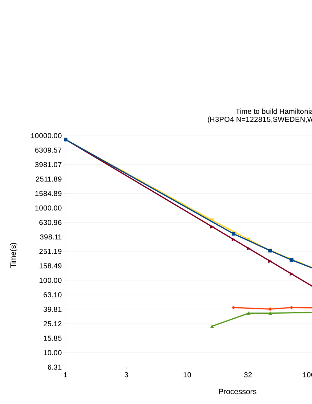
Figure 8: Time taken (log scale) to build the scattering Hamiltonian for phosphoric acid against process counts (log scale). The size of the Hamiltonian is $N=122815$. The ideal time is computed using Eq. 13. The update+IO time is the time taken for MPI synchronization steps that include disk writes by the WriterMatrix. The time taken by MPI-SCATCI includes the update+IO time.

For phosphoric acid, the build phase requires between 1 to 3 nodes for maximum efficiency and reduces the calculation from hours to minutes with higher counts considered overkill. However a higher process count would still be beneficial if one wishes to perform diagonalization afterwards.

4.2 Beryllium mono-hydride

The Beryllium mono-hydride (BeH) [24] calculation is a contraction heavy calculation. The contracted portion of the matrix is of dimension 10104 and the $L^{2}$ portion is of dimension 20563 giving a total dimension of $N=30667$. Whilst this matrix is significantly smaller than phosphoric acid, it acts as a better system for assessing the scaling of the heavier contraction calculation with its higher number of target symmetries (4) and with $\approx 19$ target states per target symmetry. The total storage space required for the integrals was 3.0 GB. Using shared memory, the cost to each processor was only 128-196 MB. The reference serial SCATCI time is $T_{0}=$1993.6 s. A serial single core run on MPI-SCATCI gives a time of 1154 s, a 58% improvement from SCATCI.

Figure 9 shows the performance scaling for the BeH calculation with a reference single core time $T_{0}=$1993.6 s.

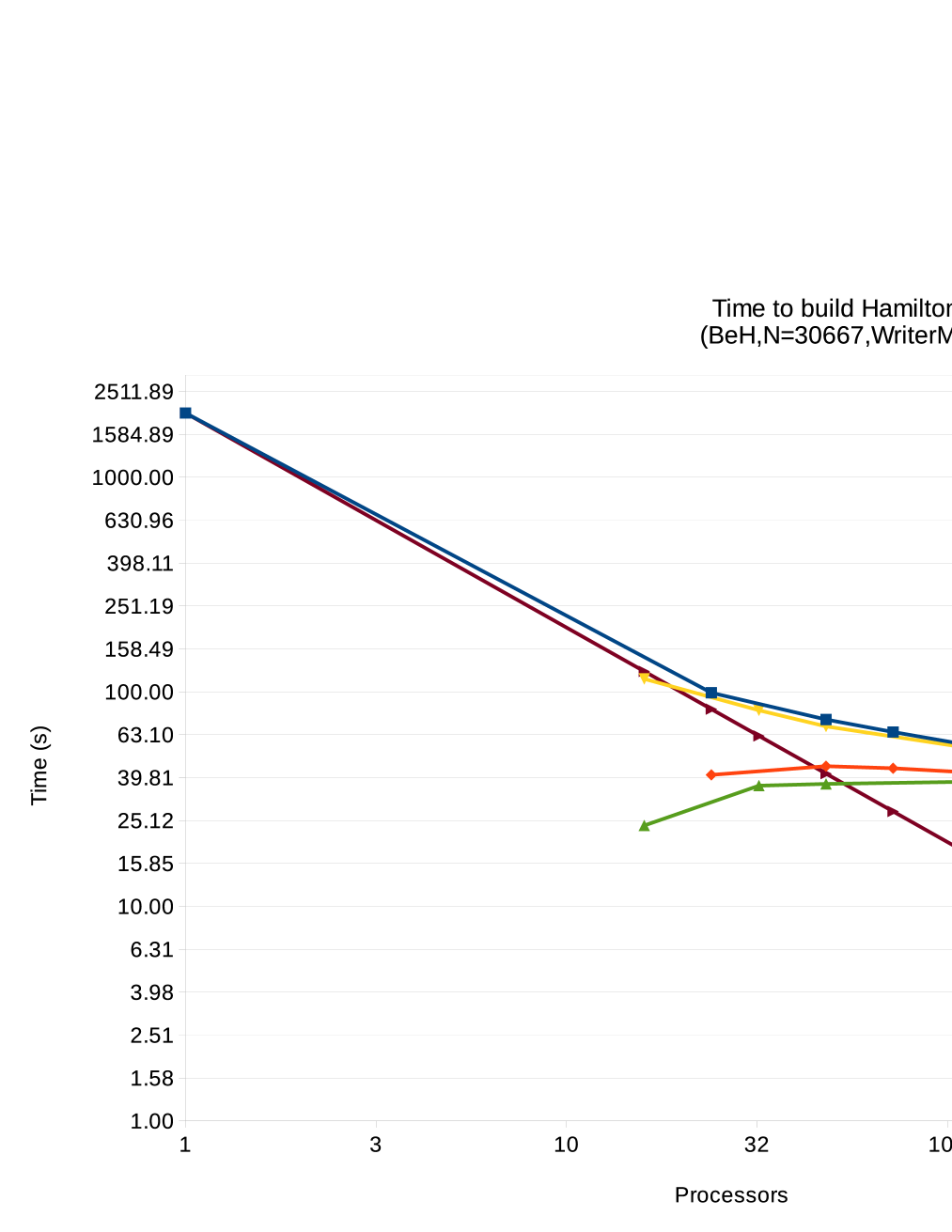
Figure 9: Time taken (log scale) to build the scattering Hamiltonian for BeH against process counts (log scale). The size of the Hamiltonian is $N=30667$. The ideal time is computed using Eq. 13. The update+IO time is the time taken for MPI synchronization steps that include disk writes by the WriterMatrix. The time taken by MPI-SCATCI includes the update+IO time.

Almost identically to phosphoric acid, the single node ARCHER run corresponds to a speed up of $\approx$ 20 times and a parallel efficiency of $\approx$ 84%. The Grace@UCL single node run gives a 17.3 times speed up giving a $>$100 % parallel efficiency. However, the parallel efficiency drops almost immediately past this core count. This again arises from the update time comprising the majority of the calculation past this point. At 1200 cores the total time has converged with the update time. Interestingly the baseline update time also remains constant across core counts and only increases by 10 % from phosphoric acid. This comes from the increased number of target symmetries that require the prototype symbols to be synchronized for the contracted classes sans class 4. The constant behaviour of this across high process counts may come from the fact that the number of prototype symbols are in the order of thousands and the parallelization reduces this to tens of symbols for each process. These likely fit into a single packet for the interconnect. Therefore the cost may only come from the latency of the interconnect itself which is in the order of nanoseconds. Again, a single node may be considered the sweet spot for build efficiency for BeH and higher counts benefiting diagonalization.

Grace@UCL in general has a slightly lower update time, but this is most likely due to better disk IO as its single node update time is $\approx$ 30 % better than its $>1$ node performance. Running a smaller scale test on BeH with 8-12 cores over 1Gbps Ethernet, update times are 91.1 s and 171 s respectively. Considering that the resulting Hamiltonian is $\approx$ 5.6 GB, the update message moving between nodes can be as big as 1 GB, oversaturating the interconnect bandwidth. Since both Infiniband interconnects are in the realm of $\approx$ 50 Gbps, and that each core is limited to a maximum of $\approx$ 2 GB of matrix elements, the Infiniband bandwidth is not fully utilized. Therefore it is most likely the IO bandwidth that is limiting the synchronization time. This is most apparent when using a SCALAPACK Matrix as it only requires a look-up and insertion into an array. For both GRACE and ARCHER, the update times for this matrix type is around $\approx$ 17.2 s.

For both examples, the overall behaviour of the code is that the parallel efficiency is determined by the percentage of the total time taken by the update. In a sense, the update for both matrices is unaffected by core count. The greatest benefit of the code may lie in problems in the order of millions or tens of millions that take days or months to complete. High core counts may reduce these calculations to hours which would still remain significantly greater than the update time.

5 Conclusion

The UKRMol code SCATCI has been rewritten to modern standards with MPI integrated for large parallel build and diagonalization. It exploits OOP paradigms to provide flexibility for future development. A parallelization of the efficient algorithm provided by Tennyson [8] reduces a 3 hour-long calculation on phosphoric acid to several tens of seconds with only 1-3 nodes. It works by integrating several new parallel algorithms for each class to exploit their particular contraction behaviour in order to achieve a high degree of efficiency. Additionally the code supports LAPACK, ARPACK, SCALAPACK and SLEPc diagonalizers and has the ability to support many more if desired with only a few lines of code.

Use of the R-Matrix with pseudo-states (RMPS) method can rapidly lead to desirable cases where the matrix build is both large (1,000,000+) and computationally demanding [23]. Such calculations, which are important to model polarization effects in a truly ab initio manner [44], are the key for studying low-lying resonances in systems such as electron-uracil. Such calculations are currently underway.

This article has focused heavily on electron - molecule scattering aspects of the UK Molecular R-matrix codes. In fact MPI-SCATCI can be used to address other problems. A powerful but not greatly used aspect of the codes is for the studies of high-lying but bound Rydberg states of molecules. Studies have shown the use of scattering wavefunctions provides a much more efficient means of identifying these states than standard quantum-chemistry electronic structure calculations [45]. The UKRMol codes are also being increasingly used to study photoionisation [46, 47, 48, 49] and photodetachment [50]. This use raises an important technical issue with the SCATCI algorithm since the contracted Hamiltonian is based on the use of very lengthy strings of effective configuration state functions (CSFs). These CSFs, which represent entire target CI wavefunctions, do not obey the standard Slater’s rules. This means their use in computing the transition dipole moment matrix elements required for photon-driven processes requires special algorithms. Harvey et al [46] have implemented such an algorithm for SCATCI and we anticipate MPI-SCATCI being extensively used for future calculations on processes involving photons.

6 Acknowledgements

This work was funded under the embedded CSE programme of the ARCHER UK National Supercomputing Service (http://www.archer.ac.uk) as project eCSE08-7. The authors acknowledge the use of the UCL Grace High Performance Computing Facility (Grace@UCL), and associated support services, in the completion of this work. We thank Jimena Gorfinkiel and Zdenek Masin for helpful discussions, and Daniel Darby-Lewis and Kalyan Chakrabarti for help with input files. AFA would also like to thank Dr. Faris N. Al-Refaie, Lamya Ali, Sarfraz and Eri Aziz, and Rory and Annie Gleeson for their support.

References

- [1] K. Bartschat, M. J. Kushner, Electron collisions with atoms, ions, molecules, and surfaces: Fundamental science empowering advances in technology, Proc. Nat. Acad. Sci. 113 (2016) 7026–7034. doi:{10.1073/pnas.1606132113}.
- [2] J. Tennyson, A. Faure, Electron-driven processes in space, in: Gas Phase Chemistry in Space: From elementary particles to complex organic molecules, IOPP, Bristol, UK, 2017.
- [3] B. Boudaïffa, P. Cloutier, D. Hunting, M. A. Huels, L. Sanche, Resonant Formation of DNA Strand Breaks by Low-Energy (3 to 20 eV) Electrons, Science 287 (2000) 1658–1660. doi:10.1126/science.287.5458.1658.
- [4] K. Bartschat, J. Tennyson, O. Zatsarinny, Quantum-mechanical calculations of cross sections for electron collisions with atoms and molecules, Plasma Proc. Polymers 14 (2017) 1600093. doi:10.1002/ppap.201600093.
- [5] K. Bartschat, The R-matrix with pseudo-states method: Theory and applications to electron scattering and photoionization, Computer Phys. Comm. 114 (1998) 168–182.
- [6] J. D. Gorfinkiel, J. Tennyson, Electron-H collisions at intermediate energies, J. Phys. B: At. Mol. Opt. Phys. 37 (2004) L343–L350.
- [7] J. D. Gorfinkiel, J. Tennyson, Electron impact ionisation of small molecules at intermediate energies: the R-matrix with pseudostates method, J. Phys. B: At. Mol. Opt. Phys. 38 (2005) 1607–1622.
- [8] J. Tennyson, A new algorithm for Hamiltonian matrix construction in electron-molecule collision calculations, J. Phys. B: At. Mol. Opt. Phys. 29 (1996) 1817–1828.
- [9] C. J. Gillan, J. Tennyson, P. G. Burke, The UK molecular R-matrix scattering package: a computational perspective, in: W. Huo, F. A. Gianturco (Eds.), Computational methods for Electron-molecule collisions, Plenum, New York, 1995, pp. 239–254.
- [10] L. A. Morgan, J. Tennyson, C. J. Gillan, The UK molecular R-matrix codes, Comput. Phys. Commun. 114 (1998) 120–128.
- [11] J. M. Carr, P. G. Galiatsatos, J. D. Gorfinkiel, A. G. Harvey, M. A. Lysaght, D. Madden, Z. Mašín, M. Plummer, J. Tennyson, The ukrmol program suite, Eur. Phys. J. D 66 (2012) 58.
- [12] J. Tennyson, D. B. Brown, J. J. Munro, I. Rozum, H. N. Varambhia, N. Vinci, Quantemol-n: an expert system for performing electron molecule collision calculations using the r-matrix method, J. Phys. Conf. Ser. 86 (2007) 012001.
- [13] Z. Mašín, The UKRMol+ codes (2016).
- [14] D. A. Little, J. Tennyson, An R-matrix study of singlet and triplet continuum states of N2, J. Phys. B: At. Mol. Opt. Phys. 47 (2014) 105204.
- [15] S. Kaur, K. L. Baluja, Electron-impact study of SiN using the R-matrix method, Eur. Phys. J. D 69 (2015) 89. doi:10.1140/epjd/e2015-50530-1.
- [16] M. M. Fujimoto, E. V. R. de Lima, J. Tennyson, Low-energy electron collisions with CH3CN and CH3NC isomers, Eur. Phys. J. D 69 (2015) 153. doi:10.1140/epjd/e2015-60189-1.
- [17] A. Dora, L. Bryjko, T. van Mourik, J. Tennyson, R-matrix calculation of low-energy electron collisions with uracil, J. Chem. Phys. 130 (2009) 164307.
- [18] Z. Masin, J. D. Gorfinkiel, Resonance formation in low energy electron scattering from uracil, Eur. Phys. J. D 68 (2014) 112. doi:{10.1140/epjd/e2014-40797-y}.
- [19] Z. Mašín, J. D. Gorfinkiel, Effect of the third resonance on the angular distributions for electron-pyrimidine scattering, Eur. Phys. J. D 70 (2016) 151. doi:10.1140/epjd/e2016-70165-x.
- [20] K. L. Baluja, R. Zhang, J. Franz, J. Tennyson, Low-energy positron collisions with water: elastic and rotationally inelastic scattering, J. Phys. B: At. Mol. Opt. Phys. 40 (2007) 3515–3524.
- [21] R. Zhang, K. L. Baluja, J. Franz, J. Tennyson, Positron collisions with molecular hydrogen: cross sections and annihilation parameters calculated using the -matrix with pseudo-states method, J. Phys. B: At. Mol. Opt. Phys. 44 (2011) 035203.
- [22] R. Zhang, P. G. Galiatsatos, J. Tennyson, Positron collisions with acetylene calculated using the R-matrix with pseudo-states method, J. Phys. B: At. Mol. Opt. Phys. 44 (2011) 195203.
- [23] G. Halmová, J. D. Gorfinkiel, J. Tennyson, Low and intermediate energy electron collisions with the C molecular anion, J. Phys. B: At. Mol. Opt. Phys. 41 (2008) 155201.
- [24] D. Darby-Lewis, Z. Masin, J. Tennyson, R-Matrix Calculations of electron-impact electronic excitation of BeH, J. Phys. B: At. Mol. Opt. Phys.
- [25] J. Tennyson, Partitioned R-matrix theory for molecules, J. Phys. B: At. Mol. Opt. Phys. 37 (2004) 1061–1071.
- [26] J. Tennyson, Electron - molecule collision calculations using the R-matrix method, Phys. Rep. 491 (2010) 29–76.
- [27] B. Liu, M. Yoshimine, The alchemy configuration-interaction method .1. the symbolic matrix-method for determining elements of matrix operators, J. Chem. Phys. 74 (1981) 612–616.
- [28] M. Yoshimine, CONSTRUCTION OF HAMILTONIAN MATRIX IN LARGE CONFIGURATION INTERACTION CALCULATIONS, J. Comput. Phys. 11 (1973) 449–454.
- [29] L. A. Morgan, J. Tennyson, Electron impact excitation cross sections for CO, J. Phys. B: At. Mol. Opt. Phys. 26 (1993) 2429–2441.
- [30] A. Scemama, E. Giner, An efficient implementation of Slater-Condon rules, ArXiv e-printsarXiv:1311.6244.
- [31] J. D. Gorfinkiel, L. A. Morgan, J. Tennyson, Electron impact dissociative excitation of water within the adiabatic nuclei approximation, J. Phys. B: At. Mol. Opt. Phys. 35 (2002) 543–555.
- [32] E. Anderson, Z. Bai, C. Bischof, S. Blackford, J. Demmel, J. Dongarra, J. Du Croz, A. Greenbaum, S. Hammarling, A. McKenney, D. Sorensen, LAPACK Users’ Guide, 3rd Edition, Society for Industrial and Applied Mathematics, Philadelphia, PA, 1999.
- [33] R. B. Lehoucq, D. C. Sorensen, C. Yang, ARPACK Users’ Guide: Solution of Large-scale Eigenvalue Problems with Implicitly Restarted Arnoldi Methods (Software, Environments and Tools), Society for Industrial & Applied Mathematics, U.S., 1998, see http://www.caam.rice.edu/software/ARPACK/.
- [34] J. Tennyson, P. G. Burke, K. A. Berrington, Generation of continuum orbitals for molecular R-matrix calculations using lagrange orthogonalisation, Comput. Phys. Commun. 47 (1987) 207–212.
- [35] L. A. Morgan, C. J. Gillan, J. Tennyson, X. Chen, R-matrix calculations for polyatomic molecules: electron scattering by N2O, J. Phys. B: At. Mol. Opt. Phys. 30 (1997) 4087–4096.
- [36] D. T. Stibbe, J. Tennyson, Ab initio calculations of vibrationally resolved resonances in electron collisions with H2, HD and D2, Phys. Rev. Lett. 79 (1997) 4116–4119.
- [37] A. E. Orel, T. N. Rescigno, B. H. Lengsfield III, Dissociative excitation of HeH+ by electron-impact, Phys. Rev. A 44 (1991) 4328–4335.
- [38] C. J. Gillan, J. Tennyson, B. M. McLaughlin, P. G. Burke, Low energy electron impact excitation of the nitrogen molecule: optically forbidden transitions, J. Phys. B: At. Mol. Opt. Phys. 29 (1996) 1531–1547.
- [39] J. Tennyson, Phase factors in electron-molecule collision calculations, Comput. Phys. Commun. 100 (1997) 26–30.
- [40] L. S. Blackford, J. Choi, A. Cleary, E. D’Azevedo, J. Demmel, I. Dhillon, J. Dongarra, S. Hammarling, G. Henry, A. Petitet, K. Stanley, D. Walker, R. C. Whaley, ScaLAPACK Users’ Guide, Society for Industrial and Applied Mathematics, Philadelphia, PA, 1997.
- [41] V. Hernandez, J. E. Roman, V. Vidal, SLEPc: A scalable and flexible toolkit for the solution of eigenvalue problems, ACM Trans. Math. Software 31 (3) (2005) 351–362.
- [42] A. Stathopoulos, C. F. Fischer, A DAVIDSON PROGRAM FOR FINDING A FEW SELECTED EXTREME EIGENPAIRS OF A LARGE, SPARSE, REAL, SYMMETRICAL MATRIX, Comput. Phys. Commun. 79 (1994) 268–290. doi:{10.1016/0010-4655(94)90073-6}.
- [43] L. Bryjko, T. van Mourik, A. Dora, J. Tennyson, -matrix calculation of low-energy electron collisions with phosphoric acid, J. Phys. B: At. Mol. Opt. Phys. 43 (2010) 235203.
- [44] M. Jones, J. Tennyson, On the use of pseudostates to calculate molecular polarizabilities, J. Phys. B: At. Mol. Opt. Phys. 43 (2010) 045101.
- [45] D. A. Little, J. Tennyson, Singlet and triplet ab initio Rydberg states of N2, J. Phys. B: At. Mol. Opt. Phys. 46 (2013) 145102.
- [46] A. G. Harvey, D. S. Brambila, F. Morales, O. Smirnova, An R-matrix approach to electron-photon-molecule collisions: photoelectron angular distributions from aligned molecules, J. Phys. B: At. Mol. Opt. Phys. 47 (2014) 215005. doi:{10.1088/0953-4075/47/21/215005}.
- [47] A. Rouzee, A. G. Harvey, F. Kelkensberg, D. Brambila, W. K. Siu, G. Gademann, O. Smirnova, M. J. J. Vrakking, Imaging the electronic structure of valence orbitals in the XUV ionization of aligned molecules, J. Phys. B: At. Mol. Opt. Phys. 47 (2014) 124017. doi:{10.1088/0953-4075/47/12/124017}.
- [48] D. S. Brambila, A. G. Harvey, Z. Masin, J. D. Gorfinkiel, O. Smirnova, The role of multichannel effects in the photoionization of the NO2 molecule: an ab initio R-matrix study, J. Phys. B: At. Mol. Opt. Phys. 48 (2015) 245101. doi:{10.1088/0953-4075/48/24/245101}.
- [49] W. J. Brigg, A. G. Harvey, A. Dzarasova, S. Mohr, D. S. Brambila, F. Morales, O. Smirnova, J. Tennyson, Calculated photoionization cross sections using Quantemol-N, Jap. J. Appl. Phys. 54 (2015) 06GA02.
- [50] M. Khamesian, N. Douguet, S. F. dos Santos, O. Dulieu, M. Raoult, W. J. Brigg, V. Kokoouline, Formation of CN-, C3N-, and C5N- Molecules by Radiative Electron Attachment and their Destruction by Photodetachment, Phys. Rev. Lett. 117 (2016) 123001. doi:{10.1103/PhysRevLett.117.123001}.