Balancing Communication and Computation in Distributed Optimization

Abstract

Methods for distributed optimization have received significant attention in recent years owing to their wide applicability in various domains including machine learning, robotics and sensor networks. A distributed optimization method typically consists of two key components: communication and computation. More specifically, at every iteration (or every several iterations) of a distributed algorithm, each node in the network requires some form of information exchange with its neighboring nodes (communication) and the computation step related to a (sub)-gradient (computation). The standard way of judging an algorithm via only the number of iterations overlooks the complexity associated with each iteration. Moreover, various applications deploying distributed methods may prefer a different composition of communication and computation.

Motivated by this discrepancy, in this work we propose an adaptive cost framework which adjusts the cost measure depending on the features of various applications. We present a flexible algorithmic framework, where communication and computation steps are explicitly decomposed to enable algorithm customization for various applications. We apply this framework to the well-known distributed gradient descent (DGD) method, and show that the resulting customized algorithms, which we call DGD^t, NEAR-DGD^t and NEAR-DGD⁺, compare favorably to their base algorithms, both theoretically and empirically. The proposed NEAR-DGD⁺ algorithm is an exact first-order method where the communication and computation steps are nested, and when the number of communication steps is adaptively increased, the method converges to the optimal solution. We test the performance and illustrate the flexibility of the methods, as well as practical variants, on quadratic functions and classification problems that arise in machine learning, in terms of iterations, gradient evaluations, communications and the proposed cost framework.

I Introduction

The problem of optimizing an objective function by employing a distributed procedure using multiple agents in a connected network has gained significant attention over the last years. This is motivated by its wide applicability to many important engineering and scientific domains such as, wireless sensor networks [1, 2, 3, 4], multi-vehicle and multi-robot networks [5, 6, 7], smart grids [8, 9] and machine learning [10, 11]. In such problems, each agent (or node) has access to a component of the overall objective function and can only communicate with its neighbors in the underlying network. The collective goal is to minimize the summation of individual components. Formally, the system-wide problem can be represented as

$$\min_{x\in\mathbb{R}^{p}}\quad h(x)=\sum_{i=1}^{n}f_{i}(x),$$ (I.1)

where $n$ represents the number of agents in the network, convex function $h:\mathbb{R}^{p}\rightarrow\mathbb{R}$ is the global objective function, convex function $f_{i}:\mathbb{R}^{p}\rightarrow\mathbb{R}$ for each $i\in\{1,2,...,n\}$ is the local objective function available only to node $i$, and vector $x\in\mathbb{R}^{p}$ is the decision variable that the agents are optimizing cooperatively. This setup naturally calls for distributed (optimization) algorithms, where the agents iteratively perform local computations based on a local objective function and local communications, i.e., information exchange with their immediate neighbors in the underlying network, to solve the system-wide problem (I.1).

In order to decouple the computation of individual agents, problem (I.1) is often reformulated as the following consensus optimization problem by introducing a local copy $x_{i}\in\mathbb{R}^{p}$ for each agent $i\in\{1,2,...,n\}$ [12, 13],

$$\min_{x_{i}\in\mathbb{R}^{p}} \quad\sum_{i=1}^{n}f_{i}(x_{i})$$ (I.2)

s.t. $$\quad x_{i}=x_{j},\quad\forall i,j\in\mathcal{N}_{i},$$

where $\mathcal{N}_{i}$ denotes the set of neighbors of agent $i$. In this formulation, the local objective function of the $i^{th}$ agent only depends on the local copy $x_{i}$. An equality constraint, often referred to as the consensus constraint, is imposed to enforce that the local copies of neighboring nodes are equal. Since the underlying network is connected and the consensus constraint ensures that all local copies are equal, problems (I.1) and (I.2) are equivalent.

While there is a proliferating literature on developing distributed optimization methods for the above problem, most follow the conventional approach of tracking the number of iterations to judge the efficiency of a distributed algorithm, i.e., the best algorithm achieves optimality in the minimal number of iterations, and overlook the complexity associated with each iteration. In this work, we propose an alternative metric, an adaptive cost framework (in Section II) to account for the different environments and hardware constraints of various applications, where distributed optimization methods are used. In this new cost framework, we consider communication and computation costs separately and weigh them using parameters specific to the environment. This cost framework also motivates our development of a class of flexible distributed methods, where we decompose communication and computation steps. This new class of algorithms is then customizable depending on the application.

I-A Literature Review

Our work is related to the growing literature on distributed algorithms for solving problem (I.2). We outline the various lines of research next. One class of methods build upon the seminal works [12, 14], which proposed a parallel computation framework. In [13], the authors introduced a first-order primal iterative method, known as distributed (sub)-gradient descent (DGD). In one step of DGD, each agent updates its estimate of the solution via a linear combination of a gradient descent step with respect to its local objective function and a weighted average with local neighbors (also known as a consensus step). A number of later contributions [15, 16, 17, 18, 19, 20, 21, 22, 23, 24, 25, 26, 27, 28, 29, 30] extended DGD to other settings, including stochastic networks, constrained problems, and noisy environments. Coordinate descent type methods, in either primal or dual space, have also been used in the distributed setting [31, 32, 33]. Another line of research is based on Nesterov’s dual averaging algorithm [34], whose distributed version was proposed and analyzed in [10]. Dual decomposition based methods have also recently gained much attention. This class of methods includes augmented Lagrangian methods and Alternating Direction Method of Multiplier (ADMM) [35, 36, 37, 38, 39, 40, 41, 42, 3, 43, 44, 45, 46]. The last category includes second-order methods, where Newton-type methods are used to obtain faster rates of convergence [47, 48, 49, 50]. All these methods adopt the standard iteration count metric.

Closely related to our work are a few very recent contributions that incorporate communication considerations in the design of distributed algorithms [51, 52, 53, 54, 55, 56]. In [52, 53, 55, 56], the goal was to develop one particular method, where the number of communication steps is reasonable compared to the iteration complexity. While these methods are communication-efficient (with respect to some metric), they lack the flexibility to adapt to different environments. In [51], the authors consider how to design a network topology that is communication-efficient, assuming the network topology can be controlled. The closest work to ours is [54]. In this recent work, the authors control the frequency of communication steps and analyze the time performance of a dual averaging based algorithm. The goal of [54] was to show that speed-up is possible when the agents communicate less frequently. While this work pioneers the idea of adjusting the relative frequencies of communication and computation, it focuses solely on reducing the runtime of the algorithm and overlooks other important aspects, such as energy consumption.

In this paper, in order to demonstrate our new cost framework (II.1), we consider decoupling the communication and computation steps of the well-studied DGD method and vary the frequency of these steps. On this front, our work is related to [57, 58, 17]. In [58], the authors propose to increase the number of communication steps at rate $k$, where $k$ is the number of iterations, to ensure convergence with a fixed stepsize (aka steplength) for proximal gradient-based algorithms on composite nonsmooth convex problems. In [17], the authors extended this idea to smooth problems and propose to increase communication at rate $\log(k)$.

In [57], the author propose two algorithms for quadratic problems: CTA (Combine-then-Adapt) and ATC (Adapt-then-Combine). Both of these methods stem from a new way of combining communication and computation steps and they differ in the order that the consensus and gradient operations are performed. While our method employs a similar way to decompose and combine communication and computation steps, our method is not restricted to using exactly one consensus step and one gradient step at each iteration. Hence, it is more general and offers flexibility in how to combine these steps. In particular, our convergence guarantee holds for many different ways of increasing the frequency of communication including $k$ and $\log(k)$, as appeared in [58] and [17], respectively.

One major problem of the standard DGD method is that it only converges to a neighborhood of the optimal solution when a constant stepsize is employed. Recently, there have been many new distributed algorithms [29, 59, 60, 61, 62, 47] that can achieve exact convergence with a constant stepsize. In [29, 61, 60, 47], the authors also show their respective algorithms can achieve a linear rate of convergence. Our work is also related to this line of literature as many instances of our proposed class of algorithms achieve exact convergence. Moreover, one instance of our method converges linearly with respect to number of gradient computations, and sublinearly with respect to number of communications or our cost framework. While the proposed method has many similarities with the existing algorithms, it also boasts unique flexibility and adaptability.

I-B Contributions

Our innovations in this paper are on two fronts: (i) the new adaptive cost framework, and (ii) the proposed class of flexible algorithms motivated by this framework. We next describe our main contributions:

• We introduce a metric of performance based on the weighted combination of costs of both communication and computation steps. This metric is adaptive to, and can accurately characterize, different features of the application environments independent of the distributed algorithms.

• We decompose the communication and computation steps of DGD to enable algorithm customization. Based on this, we propose three classes of related flexible algorithms, which we call DGD^t, NEAR-DGD^t and NEAR-DGD⁺. We can tune the instances in these classes to balance the communication and computation costs according to the application.

• We develop a class of exact first-order methods with constant stepsize (NEAR-DGD⁺), based on nesting the communication and computation steps, and increasing the number of consensus steps performed as the algorithm evolves. When we increase the number of consensus steps at rate $k$, where $k$ is the number of iterations, then we obtain an algorithm that achieves exact convergence at a linear rate. In particular, to get an $\epsilon$-accurate solution, we need $\mathcal{O}(\log(\nicefrac{{1}}{{\epsilon}}))$ numbers of gradient computations and $\mathcal{O}(\log(\nicefrac{{1}}{{\epsilon}})^{2})$ number of communication rounds.

• We illustrate the empirical performance of some instances of the proposed class of methods on quadratic and logistic regression problems as measured by our new cost framework. We also demonstrate some practical instances of the class of methods that perform very well in practice in terms of iterations, number of communications, number of gradients and combined cost.

In summary, our main contribution is the proposed cost framework in conjunction with the decomposition of the communication and computation steps. This allows for flexibility in algorithmic design, for a class of theoretically sound and efficient algorithms, and the first step towards harmonization of the communication and computation costs.

The paper is organized as follows. In Section II we describe in detail our proposed cost framework. Section III reviews relevant distributed optimization preliminaries such as reformulations of (I.2), and the DGD method. The variant of DGD method with multiple consensus steps, which we call DGD^t, is introduced and analyzed in Section IV. In Section V, we describe the new NEAR-DGD^t and NEAR-DGD⁺ methods, provide theoretical analysis of the variants and also present numerical results. We provide some final remarks and future directions of research in Section VI.

II Adaptive Cost Framework

A typical iteration of a distributed optimization method consists of some local computation (typically gradient or Hessian evaluation) and neighborhood communication. While the amount of computation and communication per iteration differs from one algorithm to another, all iterations are counted blindly as equal in the traditional iteration counting metric. Moreover, as distributed algorithms are deployed in various contexts, the diverse range of scenarios calls for different ways to account for the cost (in terms of time, energy, or any other metric) of an algorithm. To illustrate this we discuss two motivating examples. Consider first the problem of controlling a swarm of battery powered robots, with low-energy computation modules onboard, connected via an energy-intense communication protocol. Since the robots have limited energy supply, communication steps can be very expensive, while longer task completion times may not be problematic. On the other hand, we consider solving a large-scale machine learning problem on a cluster of computers that are physically connected or with shared memory access. In this case, the cost of communication can be ignored (inexpensive in terms of time), while the computational cost (time) can be expensive depending on the size of the data set on each machine. Hence, a desirable metric should not only count the total number of communication and computation steps, it should also weigh the two appropriately according to different environments.

We propose an adaptive cost framework to evaluate the performance of distributed optimization methods which explicitly accounts for the cost of communication and computation, and can be customized depending on the specific application. In particular, we propose the following simple yet powerful metric

$$\text{Cost}=\#\text{Communications}\times c_{c}+\#\text{Computations}\times c_{g},$$ (II.1)

where $c_{c}$ and $c_{g}$ are exogenous application-dependent parameters reflecting the costs of communication and computation, respectively. For instance, when energy is the most constraining resource of the environment, the parameters $c_{c}$ and $c_{g}$ would reflect the energy consumed per step of communication/computation. Similarly, when the runtime is of concern, the parameters would correspond to the time needed for a communication/computation step. This cost could also represent some combination of time and energy. In the battery powered robots example we would have $c_{c}>c_{g}$, and in the machine learning example we would have $c_{c}<c_{g}$. We note that if the cost of communication and computation of one iteration is $1$, then to design an algorithm with minimal cost reduces to the standard problem of finding algorithm with the least iteration count.

III Preliminaries

In this section, we introduce an equivalent compact reformulation of problem (I.2) and review the basics of the DGD method, both of which will be used to build our class of flexible algorithms.

III-A Equivalent Reformulations

For compactness, we express problem (I.2) as

$$\min_{x_{i}\in\mathbb{R}^{p}} \quad f(\textbf{x})=\sum_{i=1}^{n}f_{i}(x_{i})$$ (III.1)

s.t. $$\quad(\textbf{W}\otimes I_{p})\textbf{x}=\textbf{x}$$

where $\textbf{x}\in\mathbb{R}^{np}$ is a concatenation of all local $x_{i}$’s and W is a matrix of size $\mathbb{R}^{n\times n}$, i.e.,

$$\textbf{x}=\begin{bmatrix}x_{1}\\ x_{2}\\ \vdots\\ x_{n}\end{bmatrix},\quad\textbf{W}=\begin{bmatrix}w_{11}&w_{12}&\cdots&w_{1n}\\ w_{21}&w_{22}&\cdots&w_{2n}\\ \vdots&\vdots&\ddots&\vdots\\ w_{n1}&w_{n2}&\cdots&w_{nn}\end{bmatrix}.$$

Matrix $I_{p}$ is the identity matrix of dimension $p$, and the operator $\otimes$ denotes the Kronecker product operation, with $\textbf{W}\otimes I_{p}\in\mathbb{R}^{np\times np}$. Moreover, matrix W has the following properties: it is symmetric, doubly-stochastic, with diagonal elements $w_{ii}>0$ and off-diagonal elements $w_{ij}>0$ ($i\neq j$) if and only if $i$ and $j$ are neighbors in the underlying communication network. Matrix W is known as the consensus matrix and it has the property that $(\textbf{W}\otimes I_{p})\textbf{x}=\textbf{x}$ if and only if $x_{i}=x_{j}$ for all $i$ and $j$ in the connected network [13], i.e., problems (I.2) and (III.1) are equivalent. We also have that matrix W has exactly one eigenvalue equal to 1 and the rest of eigenvalues have absolute values strictly less than 1. We use $\beta$, with $0<\beta<1$, to denote the second largest magnitude of the eigenvalues of W. For the rest of the paper, we focus on developing methods to solve problem (III.1).

III-B Distributed Gradient Descent

We now review the basic Distributed Gradient Descent (DGD) method [13], which is the building block for our later development of the DGD^t, NEAR-DGD^t and NEAR-DGD⁺ methods. The DGD method is a first-order method for solving problem (III.1), where each agent updates its local estimate iteratively using a gradient based on local information and information exchanged with its neighbors in the network. The $k^{th}$ iteration of the DGD method for any node $i$ can be expressed as

$$x_{i,k+1}=\sum_{j\in\mathcal{N}_{i}\cup\{i\}}w_{ij}x_{j,k}-\alpha\nabla f_{i}(x_{i,k}),\qquad\forall i=1,\ldots,n,$$

where $x_{i,k}$ represents the local estimate of agent $i$ at iteration $k$ and the positive scalar $\alpha$ denotes the stepsize. Effectively, the $i^{th}$ agent computes a weighted average of its and its neighbors local estimates, and takes a step in the negative gradient direction obtained using only local information. Equivalently, in the concatenated notation, the DGD method can be expressed as

$$\textbf{x}_{k+1}=\textbf{Z}\textbf{x}_{k}-\alpha\nabla\textbf{f}(\textbf{x}_{k})$$ (III.2)

where

$$\nabla\textbf{f}(\textbf{x}_{k})=\begin{bmatrix}\nabla f(x_{1,k})\\ \nabla f(x_{2,k})\\ \vdots\\ \nabla f(x_{n,k})\end{bmatrix}\in\mathbb{R}^{np}$$

and the matrix $\textbf{Z}=\textbf{W}\otimes I_{p}\in\mathbb{R}^{np\times np}$.

The DGD method can also be thought of as a gradient method with unit steplength on the following convex problem

$$\min_{\textbf{x}\in\mathbb{R}^{np}}\frac{1}{2}\textbf{x}^{T}({I-\textbf{Z}})\textbf{x}+\alpha\sum_{i=1}^{n}f_{i}(x_{i}).$$ (III.3)

The theoretical properties of the DGD method have been well established; see [12, 13, 63]. The convergence results are typically established under the following standard assumptions:

Assumption III.1.

Each local objective function $f_{i}$ has $L_{i}$-Lipschitz continuous gradients.

Assumption III.2.

The objective function $h$ (I.1) is $\mu_{h}$-strongly convex.

Assumption III.3.

Each local objective function $f_{i}$ is $\mu_{i}$-strongly convex. Note, this Assumption implies Assumption III.2.

These assumptions guarantee the existence of a unique optimal solution. Under Assumption III.1, the DGD method can be shown to converge at a sublinear rate with diminishing stepsize (decrease stepsize $\alpha$ as the algorithm evolves). The diminishing stepsize is effectively shrinking the penalty parameter $\alpha$ of problem (III.3) and thus DGD recovers a feasible and optimal solution of problem (III.1) in the limit. If we further assume the conditions in Assumption III.3, then with an appropriate constant stepsize, DGD converges at a linear rate to the optimal solution of (III.3), which is in a neighborhood of the optimal solution of (III.1) [63]. The limit point of DGD with constant stepsize is often infeasible for the equality constraint in problem (III.1).

Notation: For the rest of the paper, we follow the same notation as in this section. A boldface lower case letter indicates a concatenated vector, i.e., $\textbf{v}\in\mathbb{R}^{np}$ represents the concatenation of local vectors $v_{i}\in\mathbb{R}^{p}$. Notation $\bar{v}\in\mathbb{R}^{p}$ denotes the average of all local vectors $v_{i}\in\mathbb{R}^{p}$, i.e., $\bar{v}=\frac{1}{n}\sum_{i=1}^{n}v_{i}$. The two subscripts $x_{i,k}$ indicate the agent index $i$ and iteration count $k$.

IV DGD^t: A Distributed Gradient Descent Variant

A close inspection of the DGD iterate update Eq. (III.2) reveals that the method performs a single round of communication and a single computation per iteration. However, a natural question is whether this is optimal or even necessary. Restating this question from a different angle: is there flexibility in creating a whole class of methods based on the components of the DGD method that perform different number of communication and computation steps depending on the application? Motivated by this question and our adaptive cost framework (Section II), we decompose and rearrange the communication and computation steps of DGD to construct more flexible algorithms. We present two improved classes of DGD-based algorithms in this and the following sections, which we call DGD^t and NEAR-DGD methods, respectively. We also provide answers to the following questions: (i) what the interpretation of these new methods are, and (ii) what theoretical guarantees can be established. For simplicity, we will focus on the constant stepsize implementations.

For the first class of algorithms, we consider scenarios in which communication is much cheaper than computation, as in the shared memory machine learning example. We note that a major drawback of the DGD algorithm is that to obtain a feasible solution we need to use diminishing stepsizes, which results in slow convergence speed. With constant stepsizes, the resulting solution of DGD is infeasible with respect to the equality constraint of problem (III.1). In order to improve the solution quality without sacrificing convergence speed, we propose to perform $t$ consensus steps at each iteration, and consider the following constant stepsize iterate update equation,

$$\textbf{x}_{k+1}=\textbf{Z}^{t}\textbf{x}_{k}-\alpha\nabla\textbf{f}(\textbf{x}_{k}),\qquad\textbf{Z}^{{t}}=\textbf{W}^{{t}}\otimes I_{p},$$ (IV.1)

which we call the DGD^t method. The DGD^t method can be thought of as a gradient method with unit steplength on the following convex problem

$$\min_{\textbf{x}\in\mathbb{R}^{np}}p_{f}(\textbf{x})=\frac{1}{2}\textbf{x}^{T}({I-\textbf{Z}^{t}})\textbf{x}+\alpha\sum_{i=1}^{n}f_{i}(x_{i}).$$ (IV.2)

The intuition behind this method is that by increasing the number of consensus steps from $1$ to $t$ per iteration, the resulting solution should be closer to being feasible. Alternatively, we can view the DGD^t method as a DGD method with a different underlying graph (different weights in W). As we will show next, the solution of DGD^t is indeed closer to being feasible compared to standard DGD. This is achieved at the cost of more communication steps per iteration. Also, unlike DGD, where the gradient computation and consensus can happen simultaneously, the $t$ communication steps in DGD^t have to happen sequentially. This method can be desirable when communication is cheap, i.e., $c_{c}$ is much smaller than $c_{g}$.

IV-A Convergence Analysis of DGD^t

We now provide a complete convergence analysis for the DGD^t method with constant stepsize. We should note again that DGD^t is a variant of DGD by replacing the weight matrix $W$ by $W^{t}$. As such, our analysis follows a similar approach as in [63], and so for brevity we have omitted the proofs. The proofs can be found in [64].

For notational convenience, we introduce the following quantities that are used in the analysis

$$\bar{x}_{k}=\frac{1}{n}\sum_{i=1}^{n}x_{i,k},\quad g_{k}=\frac{1}{n}\sum_{i=1}^{n}\nabla f_{i}(x_{i,k}),$$

$$\bar{g}_{k}=\frac{1}{n}\sum_{i=1}^{n}\nabla f_{i}(\bar{x}_{k}).$$ (IV.3)

Vector $\bar{x}_{k}\in\mathbb{R}^{p}$ corresponds to the average of local estimates, vector $g_{k}\in\mathbb{R}^{p}$ represents the average of local gradients at the current local estimates and vector $\bar{g}_{k}\in\mathbb{R}^{p}$ indicates the average gradient at $\bar{x}_{k}$.

Lemma IV.1.

(Bounded gradients) Suppose Assumption III.1 holds, and let the steplength satisfy

$$\alpha\leq{\frac{1+\lambda_{n}(\textbf{W}^{{t}})}{L}}$$ (IV.4)

where ${\lambda_{n}(\textbf{W}^{{t}})}$ is the smallest eigenvalue of ${\textbf{W}^{{t}}}$ and $L=\max_{i}L_{i}$. Then, starting from $x_{i,0}=0$ ($1\leq i\leq n$), the sequence $x_{i,k}$ generated by the DGD^t method converges. In addition, we also have

$$\|\nabla\textbf{f}(\textbf{x}_{k})\|\leq D=\sqrt{2L\left(\sum_{i=1}^{n}\left(f_{i}(0)-f_{i}^{\star}\right)\right)}$$

for all $k=1,2,\ldots$, where $f_{i}^{\star}=f_{i}(x_{i}^{\star})$ and $x_{i}^{\star}=\arg\min_{x}f_{i}(x)$.

Proof.

Note that the DGD^t iteration (IV.1) is equivalent to a gradient descent iteration, with unit steplength on the quadratic penalty function $p_{f}$ (IV.2). We first show that the function $p_{f}$ has $\left[\left(1-\lambda_{n}(\textbf{W}^{t})\right)+\alpha L\right]$-Lipschitz continuous gradients. By definition of $p_{f}$ and the triangle inequality, we have

$$\left|\left|\nabla p_{f}(u)-\nabla p_{f}(v)\right|\right| \leq\left|\left|(I-\textbf{Z}^{t})(u-v)\right|\right|$$

$$\quad+\alpha\left|\left|\sum_{i=1}^{n}\nabla f_{i}(u_{i})-\sum_{i=1}^{n}\nabla f_{i}(v_{i})\right|\right|.$$ (IV.5)

By the Cauchy-Schwartz inequality, the first term satisfies

$$\left|\left|(I-\textbf{Z}^{t})(u-v)\right|\right| \leq\left|\left|I-\textbf{Z}^{t}\right|\right|\left|\left|u-v\right|\right|$$

$$=\left(1-\lambda_{n}(\textbf{W}^{t})\right)\left|\left|u-v\right|\right|,$$

where the last inequality follows from the fact that all eigenvalues of the matrix W lie in the interval $(-1,1]$. The second term in Eq. (IV-A) satisfies

$$\alpha\left|\left|\sum_{i=1}^{n}\nabla f_{i}(u_{i})-\sum_{i=1}^{n}\nabla f_{i}(v_{i})\right|\right|\leq\alpha L\left|\left|u-v\right|\right|,$$

due to Assumption III.1. Thus, we have that the function $p_{f}$ has Lipschitz continuous gradients with

$$L_{p_{f}}\leq\left(1-\lambda_{n}(\textbf{W}^{t})\right)+\alpha L.$$

From the classical analysis of gradient descent [12], we know that these iterates will converge with unit stepsize if $1\leq\frac{2}{L_{p_{f}}}$, where $L_{p_{f}}$ is the Lipschitz constant of the gradients of $p_{f}$. Since $\alpha\leq{\frac{1+\lambda_{n}(\textbf{W}^{{t}})}{L}}$ from Eq. (IV.4), we have

$$L_{p_{f}} \leq\left(1-\lambda_{n}(\textbf{W}^{t})\right)+\alpha L$$

$$\leq\left(1-\lambda_{n}(\textbf{W}^{t})\right)+{\frac{1+\lambda_{n}(\textbf{W}^{{t}})}{L}}L\leq 2.$$

Hence when the condition in Eq. (IV.4) is satisfied, the iterates $\textbf{x}_{k}$ will converge which implies that the individual iterates $x_{i,k}$ converge.

We now show the bound on the gradients. Since the function values obtained in the gradient descent method are non-increasing and $I-\textbf{W}^{t}$ is a positive semi-definite matrix, we have,

$$\sum_{i=1}^{n}f_{i}(x_{i,k})\leq\frac{1}{\alpha}p_{f}(\textbf{x}_{k})\leq\frac{1}{\alpha}p_{f}(\textbf{x}_{k-1})\leq\dots$$

$$\dots\leq\frac{1}{\alpha}p_{f}(\textbf{x}_{0})=\sum_{i=1}^{n}f_{i}(0).$$ (IV.6)

By Theorem 2.1.5 in [66], any convex function $\phi$ with $L-$Lipschitz gradient satisfies

$$\phi(x)+\nabla\phi(x)^{T}(y-x)+\frac{1}{2L}\left|\left|\nabla\phi(x)-\nabla\phi(y)\right|\right|^{2}\leq\phi(y)$$

for all $x,y$ in its domain. We apply this relation to each of $f_{i}$ at respective $x_{i}^{\star}$, and have

$$f_{i}(x_{i}^{\star})+\frac{1}{2L_{i}}\left|\left|\nabla f_{i}(x)\right|\right|^{2}\leq f_{i}(x)$$ (IV.7)

for all $x$ in $\mathbb{R}^{p}$.

Finally, we can bound $\|\nabla\textbf{f}(\textbf{x}_{k})\|^{2}$ by

$$\|\nabla\textbf{f}(\textbf{x}_{k})\|^{2}=\sum_{i=1}^{n}\|\nabla f_{i}(x_{i,k})\|^{2} \leq\sum_{i=1}^{n}2L_{i}\left(f_{i}(x_{i,k})-f^{\star}_{i}\right)$$

$$\leq 2L\left(\sum_{i=1}^{n}\left(f_{i}(0)-f^{\star}_{i}\right)\right).$$

where the first inequality follows from Eq. (IV.7) and the second inequality uses the definition of $L$ and Eq. (IV-A). ∎

Lemma IV.1 shows that the iterates produced by the DGD^t method converge and have bounded gradients. A different bound can be shown if $x_{i,0}\neq 0$ for all $i$. For convenience, we assume that $x_{i,0}=0$, for all $i$ for the rest of this section.

Lemma IV.2.

(Bounded deviation from mean) If Assumptions III.1-III.2 hold. Then, starting from $x_{i,0}=0$, the total deviation from the mean is bounded, namely,

$${\|x_{i,k}-\bar{x}_{k}\|\leq\frac{\alpha D}{1-\beta^{{t}}}},$$

and

$${\|\nabla f_{i}(x_{i,k})-\nabla f_{i}(\bar{x}_{k})\|\leq\frac{\alpha DL_{i}}{1-\beta^{{t}}}},$$ (IV.8)

$${\|g_{k}-\bar{g}_{k}\|\leq\frac{\alpha DL}{1-\beta^{{t}}}},$$ (IV.9)

for all $k=1,2,\ldots$ and $1\leq i\leq n$.

Proof.

By iteratively applying the DGD^t iteration (IV.1) and the definition of x, we obtain

$$\textbf{x}_{k}=-\alpha\sum_{s=0}^{k-1}\left(\textbf{W}^{t(k-1-s)}\otimes I\right)\nabla\textbf{f}(x_{s}).$$

Let $\bar{\textbf{x}}_{k}=[\bar{x}_{k};\bar{x}_{k};\ldots;\bar{x}_{k}]\in\mathbb{R}^{np}$, it follows that

$$\bar{\textbf{x}}_{k}=\frac{1}{n}\left((1_{n}1_{n}^{T})\otimes I\right)\textbf{x}_{k}.$$

As a result,

$$\|x_{i,k}-\bar{x}_{k}\|\leq\|\textbf{x}_{k}-\bar{\textbf{x}}_{k}\|$$

$$=\left\|\textbf{x}_{k}-\frac{1}{n}\left((1_{n}1_{n}^{T})\otimes I\right)\textbf{x}_{k}\right\|$$

$$=\left\|-\alpha\sum_{s=0}^{k-1}\left(\textbf{W}^{t(k-1-s)}\otimes I\right)\nabla\textbf{f}(x_{s})\right.$$

$$\qquad+\left.\alpha\sum_{s=0}^{k-1}\frac{1}{n}\left((1_{n}1_{n}^{T}\textbf{W}^{t(k-1-s)})\otimes I\right)\nabla\textbf{f}(x_{s})\right\|$$

$$=\left\|-\alpha\sum_{s=0}^{k-1}\left(\textbf{W}^{t(k-1-s)}\otimes I\right)\nabla\textbf{f}(x_{s})\right.$$

$$\qquad+\left.\alpha\sum_{s=0}^{k-1}\frac{1}{n}\left((1_{n}1_{n}^{T})\otimes I\right)\nabla\textbf{f}(x_{s})\right\|,$$

where the third equality holds since $\textbf{W}^{t}$ is doubly-stochastic, which is a direct consequence of W being doubly-stochastic. Thus we have,

$$\|x_{i,k}-\bar{x}_{k}\| \leq\left\|-\alpha\sum_{s=0}^{k-1}\left(\textbf{W}^{t(k-1-s)}\otimes I\right)\nabla\textbf{f}(x_{s})\right.$$

$$\qquad\qquad+\left.\alpha\sum_{s=0}^{k-1}\frac{1}{n}\left((1_{n}1_{n}^{T})\otimes I\right)\nabla\textbf{f}(x_{s})\right\|$$

$$=\alpha\left\|\sum_{s=0}^{k-1}\left((\textbf{W}^{t(k-1-s)}-\frac{1}{n}1_{n}1_{n}^{T})\otimes I\right)\nabla\textbf{f}(x_{s})\right\|$$

$$\leq\alpha\sum_{s=0}^{k-1}\left\|\textbf{W}^{t(k-1-s)}-\frac{1}{n}1_{n}1_{n}^{T}\right\|\|\nabla\textbf{f}(x_{s})\|$$

$$=\alpha\sum_{s=0}^{k-1}\beta^{t(k-1-s)}\|\nabla\textbf{f}(x_{s})\|,$$

where the inequality is due to Cauchy-Schwartz, and the last equality follows from the definition of $\beta$, since the matrix $\frac{1}{n}1_{n}1_{n}^{T}$ is the projection of W onto the eigenspace associated with the eigenvalue equal to $1$. Using Lemma IV.1 and the fact that $\beta<1$, it follows that

$$\|x_{i,k}-\bar{x}_{k}\| \leq\alpha\sum_{s=0}^{k-1}\beta^{t(k-1-s)}\|\nabla\textbf{f}(x_{s})\|$$

$$\leq\alpha D\sum_{s=0}^{k-1}\beta^{t(k-1-s)}\leq\frac{\alpha D}{1-\beta^{t}}.$$ (IV.10)

The result (IV.8) is a direct consequence of (IV-A) and the Lipschitz continuity of the individual gradients (Assumption III.1). For the second result (IV.9), we have

$$\|g_{k}-\bar{g}_{k}\| =\left\|\frac{1}{n}\sum_{i=1}^{n}\left(\nabla f_{i}(x_{i,k})-\nabla f_{i}(\bar{x}_{k})\right)\right\|$$

$$\leq\frac{1}{n}\sum_{i=1}^{n}L_{i}\|x_{i,k}-\bar{x}_{k}\|\leq\frac{\alpha DL}{1-\beta^{t}}.$$

∎

Lemma IV.2 shows that the distance between the local iterates and the average is bounded. As a consequence of this, the deviation in the gradients is also bounded.

We now look at the optimization error. We observe that due to the doubly-stochastic nature of W,

$$\bar{\textbf{x}}_{k+1} =\frac{1}{n}\left((1_{n}1_{n}^{T})\otimes I\right){\textbf{x}}_{k+1}$$

$$=\frac{1}{n}\left((1_{n}1_{n}^{T})\otimes I\right)\left((\textbf{W}^{{t}}\otimes I)\textbf{x}_{k}-\alpha\nabla\textbf{f}(\textbf{x}_{k})\right)$$

$$=\frac{1}{n}\left((1_{n}1_{n}^{T}\textbf{W}^{{t}})\otimes I\right)\textbf{x}_{k}-\frac{\alpha}{n}\left((1_{n}1_{n}^{T})\otimes I\right)\nabla\textbf{f}(\textbf{x}_{k})$$

$$=[\bar{x}_{k}-\alpha g_{k};\bar{x}_{k}-\alpha g_{k};\ldots;\bar{x}_{k}-\alpha g_{k}].$$

Thus we have

$$\bar{{x}}_{k+1}=\bar{{x}}_{k}-\alpha g_{k}.$$ (IV.11)

Recall that $g_{k}$ is the average of gradients at the current local estimates [cf. Eq. (IV-A)] and thus the above equation can be viewed as an inexact gradient descent step for the problem

$$\min_{x\in\mathbb{R}^{p}}\bar{f}(x)=\frac{1}{n}\sum_{i=1}^{n}f_{i}(x),$$ (IV.12)

where $\bar{g}_{k}$ is the exact gradient (at the average of the local estimates). Consequently, if $h$ has $L_{h}$-Lipschitz continuous gradients, and is $\mu_{h}$-strongly convex, then it can be shown that the function $\bar{f}$ has $L_{\bar{f}}$-Lipschitz continuous gradients and is $\mu_{\bar{f}}$ strongly convex with

$$L_{\bar{f}}=\frac{1}{n}\sum_{i=1}^{n}L_{i}=\frac{1}{n}L_{h},\quad\mu_{\bar{f}}=\frac{1}{n}\sum_{i=1}^{n}\mu_{i}=\frac{1}{n}\mu_{h}.$$

Based on the above observations, we bound the distance to the optimal solution.

Theorem IV.3.

(Bounded distance to optimal solution) Suppose Assumptions III.1-III.2 hold, and let the steplength satisfy

$$\alpha\leq\min\left\{{\frac{1+\lambda_{n}(\textbf{W}^{{t}})}{{L}},c_{4}}\right\}$$

where ${\lambda_{n}(\textbf{W}^{{t}})}$ is the smallest eigenvalue of ${\textbf{W}^{{t}}}$, $L=\max_{i}L_{i}$ and $c_{4}=\frac{{2}}{\mu_{\bar{f}}+L_{\bar{f}}}$. Then, starting from $x_{i,0}=0$ ($1\leq i\leq n$), for all $k=0,1,2,\ldots$

$$\|\bar{x}_{k+1}-x^{\star}\|^{2}\leq c_{1}^{2}\|\bar{x}_{k}-x^{\star}\|^{2}+\frac{{{c_{3}^{2}}}}{{{(1-\beta^{{t}})^{2}}}},$$

where

$$c_{1}^{2}=1-\alpha c_{2}+\alpha\delta-\alpha^{2}\delta c_{2},\;\;c_{2}=\frac{{2}\mu_{\bar{f}}L_{\bar{f}}}{\mu_{\bar{f}}+L_{\bar{f}}},$$

$$c_{3}^{2}=\alpha^{3}(\alpha+\delta^{-1})L^{2}D^{2},\;\;D=\sqrt{2L\left(\sum_{i=1}^{n}f_{i}(0)-f^{\star}\right)},$$

$x^{\star}$ is the optimal solution of (III.1) and $\delta>0$. In particular, if we set $\delta=\frac{c_{2}}{2(1-\alpha c_{2})}$ such that $c_{1}=\sqrt{1-\frac{\alpha c_{2}}{2}}\in(0,1)$, then for $k=0,1,2,\ldots$

$$\|\bar{x}_{k}-x^{\star}\|\leq c_{1}^{k}\|\bar{x}_{0}-x^{\star}\|+\mathcal{O}\left(\frac{\alpha}{1-\beta^{t}}\right).$$

Proof.

Using the definitions of the $\bar{x}_{k}$, $g_{k}$ and (IV.11), we have

$$\|\bar{x}_{k+1}-x^{\star}\|^{2} =\|\bar{x}_{k}-x^{\star}-\alpha g_{k}\|^{2}$$

$$=\|\bar{x}_{k}-x^{\star}-\alpha\bar{g}_{k}+\alpha(\bar{g}_{k}-g_{k})\|^{2}$$

$$=\|\bar{x}_{k}-x^{\star}-\alpha\bar{g}_{k}\|^{2}+\alpha^{2}\|\bar{g}_{k}-{g}_{k}\|^{2}$$

$$\quad+2\alpha(\bar{g}_{k}-g_{k})^{T}(\bar{x}_{k}-x^{\star}-\alpha\bar{g}_{k})$$

$$\leq(1+\alpha\delta)\|\bar{x}_{k}-x^{\star}-\alpha\bar{g}_{k}\|^{2}$$

$$\quad+\alpha(\alpha+\delta^{-1})\|\bar{g}_{k}-{g}_{k}\|^{2},$$ (IV.13)

where the last inequality follows from the fact that for any vectors $a$ and $b$, $\pm 2a^{T}b\leq\delta^{-1}\|a\|^{2}+\delta\|b\|^{2}$, for $\delta>0$.

We now bound the quantity $\|\bar{x}_{k}-x^{\star}-\alpha\bar{g}_{k}\|^{2}$,

$$\| \bar{x}_{k}-x^{\star}-\alpha\bar{g}_{k}\|^{2}$$

$$=\|\bar{x}_{k}-x^{\star}\|^{2}+\alpha^{2}\|\bar{g}_{k}\|^{2}-2(\bar{x}_{k}-x^{\star})^{T}(\alpha\bar{g}_{k})$$

$$\leq\|\bar{x}_{k}-x^{\star}\|^{2}+\alpha^{2}\|\bar{g}_{k}\|^{2}-\alpha c_{4}\|\bar{g}_{k}\|^{2}-\alpha c_{2}\|\bar{x}_{k}-x^{\star}\|^{2}$$

$$=(1-\alpha c_{2})\|\bar{x}_{k}-x^{\star}\|^{2}+\alpha(\alpha-c_{4})\|\bar{g}_{k}\|^{2}$$

$$\leq(1-\alpha c_{2})\|\bar{x}_{k}-x^{\star}\|^{2},$$ (IV.14)

where the first inequality follows from [66, Theorem 2.1.12, Chapter 2], and in the last inequality we dropped the term $\alpha(\alpha-c_{4})\|\bar{g}_{k}\|^{2}$, since $\alpha\leq c_{4}$ and $\alpha(\alpha-c_{4})\|\bar{g}_{k}\|^{2}\leq 0$. By combining (IV.13) and (IV-A), and using (IV.9), we obtain

$$\|\bar{x}_{k+1}-x^{\star}\|^{2} \leq(1+\alpha\delta)(1-\alpha c_{2})\|\bar{x}_{k}-x^{\star}\|^{2}$$

$$\quad+\alpha^{3}(\alpha+\delta^{-1})\frac{L^{2}D^{2}}{(1-\beta^{{t}})^{2}}.$$ (IV.15)

Combining $c_{4}<\frac{1}{c_{2}}$, and $\alpha\leq c_{4}$, we have $(1+\alpha\delta)(1-\alpha c_{2})>0$. Now, using the definitions of $c_{1}$ and $c_{3}$, and by recursive application of (IV-A), we have Now, using the definitions of $c_{1}$ and $c_{3}$, and by recursive application of (IV-A), we have

$$\|\bar{x}_{k}-x^{\star}\|^{2} \leq c_{1}^{2k}\|\bar{x}_{0}-x^{\star}\|^{2}+\frac{c_{3}^{2}}{(1-c_{1}^{2})(1-\beta^{{t}})^{2}},$$

and so

$$\|\bar{x}_{k}-x^{\star}\| \leq c_{1}^{k}\|\bar{x}_{0}-x^{\star}\|+\frac{c_{3}}{\sqrt{1-c_{1}^{2}}(1-\beta^{{t}})}.$$

If $\delta=\frac{c_{2}}{2(1-\alpha c_{2})}>0$, then

$$c_{1}^{2}=1-\frac{\alpha c_{2}}{2}<1$$

and

$$\frac{c_{3}}{\sqrt{1-c_{1}^{2}}(1-\beta^{{t}})}=\mathcal{O}\left(\frac{\alpha}{1-\beta^{t}}\right).$$

which completes the proof. ∎

Theorem IV.3 shows that the average of the iterates generated by the DGD^t method converges to a neighborhood of the solution that is defined by the steplength, the second largest eigenvalue of W and the number of consensus steps.

Corollary IV.4.

(Local agent convergence) Suppose Assumptions III.1-III.2 hold, and let the steplength satisfy

$$\alpha\leq\min\left\{{\frac{1+\lambda_{n}(\textbf{W}^{{t}})}{L},c_{4}}\right\}.$$

where $L=\max_{i}L_{i}$ and $c_{4}=\frac{{2}}{\mu_{\bar{f}}+L_{\bar{f}}}$. Then, starting from $x_{i,0}=0$ ($1\leq i\leq n$), for $k=0,1,2,\ldots$

$$\|x_{i,k}-x^{\star}\|\leq c_{1}^{k}\|x^{\star}\|+\frac{c_{3}}{\sqrt{1-c_{1}^{2}}(1-\beta^{t})}+\frac{\alpha D}{1-\beta^{t}}.$$

Proof.

Using the results from Lemma IV.2, Theorem IV.3 and the definition of $c_{4}$, we have

$$\|x_{i,k}-x^{\star}\| \leq\|\bar{x}_{k}-x^{\star}\|+\|x_{i,k}-\bar{x}_{k}\|$$

$$\leq c_{1}^{k}\|x^{\star}\|+\frac{c_{3}}{\sqrt{1-c_{1}^{2}}(1-\beta^{t})}+\frac{\alpha D}{1-\beta^{t}}.$$

∎

The results of Theorem IV.3 and Corollary IV.4 are similar in nature to the results for the standard DGD method. More specifically, and not surprisingly, the DGD^t method converges to a neighborhood of the optimal solution of problem (III.1) when a constant steplength is employed. Compared to the DGD method, DGD^t converges to a better (smaller) neighborhood which is captured in the analysis

$$\mathcal{O}\left(\frac{1}{(1-\beta)^{2}}\right)\quad\text{v.s.}\quad\mathcal{O}\left(\frac{1}{(1-\beta^{{t}})^{2}}\right).$$

Performing multiple communication steps is beneficial as it improves the neighborhood of convergence, however, multiple consensus alone cannot guarantee convergence of the DGD^t method to the solution. Namely, the error term that appears in Theorem IV.3 cannot be eliminated by simply performing multiple rounds of communication, since $\lim_{t\rightarrow\infty}\frac{1}{(1-\beta^{{t}})^{2}}=1\neq 0$.

The results presented in Lemmas IV.1 and IV.2, Theorem IV.3 and Corollary IV.4 are not surprising, nevertheless, the results clearly illustrate the power of performing multiple rounds of communication steps.

IV-B Numerical Results for DGD^t

In this section, we provide some empirical evidence to support the theoretical results, and to ascertain that, in practice, the benefits of performing multiple consensus steps are realized. We chose a simple quadratic problem of the form

$$f(x)=\frac{1}{2}\sum_{i=1}^{n}x^{T}A_{i}x+b_{i}^{T}x,$$

where each node $i=\{1,...,n\}$ has local information $A_{i}\in\mathbb{R}^{p\times p}$ and $b_{i}\in\mathbb{R}^{p}$. The problem was constructed as described in [65]; we chose a dimension size $p=10$ and the condition number ($\kappa=\frac{L_{f}}{\mu_{f}}$) was set to $10^{2}$. For this experiment, the number of agents in the network ($n$) was $10$, and we considered a $4$-cyclic graph topology (i.e., each node is connected to its $4$ immediate neighbors).

We investigated the performance of four different variants of DGD^t, with $t=1$ (standard DGD) and $t=2,5,10$. Figure 1 illustrates the performance (relative error, $\|\bar{x}_{k}-x^{\star}\|^{2}/\|x^{\star}\|^{2}$, with $x^{\star}\neq 0$) of the four methods in terms of: (i) iterations, (ii) cost (as described in Section II, with $c_{c}=c_{g}=1$), (iii) number of gradient evaluations, and (iv) number of communications. Each of the four methods has a steplength parameter that needs to be tuned in order to achieve the best performance. We manually tuned the steplength for each method independently. We mention in passing that similar behavior was observed when we measured the performance of the methods in terms of consensus error $\left(\frac{1}{n}\sum_{i=1}^{n}\|{x}_{i,k}-x^{\star}\|^{2}/\|x^{\star}\|^{2}\right)$.

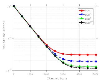
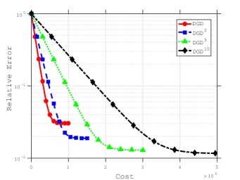
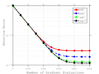
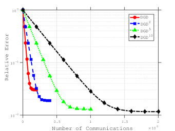
Figure 1: Performance of DGD, DGD², DGD⁵ and DGD¹⁰ measured in terms of relative error $\left(\|\bar{x}_{k}-x^{\star}\|^{2}/\|x^{\star}\|^{2}\right)$ with respect to: (i) number of iterations, (ii) cost, (iii) number of gradient evaluations, and (iv) number of communications, on a quadratic problem ($n=10$, $p=10$, $\kappa=10^{2}$).

Figure 1 clearly illustrates what was predicted by the theory. Firstly, it shows that performing multiple rounds of communication improves the neighborhood of convergence. Secondly, it shows that there is a diminishing returns effect of the number of communication rounds on the performance. Namely, the neighborhood improves substantially when going from $1$ consensus step to $2$ consensus steps, however, going from $5$ consensus steps to $10$ consensus steps has a much smaller effect. It is interesting to investigate that the performance of the methods in terms of the cost. Given a fixed cost budget, (e.g., $10^{4}$) it appears that only one method (blue: $2$ consensus steps per gradient step) is competitive with and better than the baseline DGD method. Again, the reason for this is the marginal returns effect of performing many more consensus steps per iteration. We should, of course, mention that our observation about the performance of the methods in terms of the cost are highly dependent on the cost structure that we chose for these experiments ($c_{c}=c_{g}=1$). In Section V-B, we show results for different cost structures.

Before proceeding forward we make one final remark. We tested the performance of the four methods on quadratic problems with different characteristic and different graph sizes. While the absolute performance of the methods changed, the relative performance of the methods did not. More specifically, with the cost structure $c_{c}=c_{g}=1$, similar behavior as that displayed in Figure 1 was observed.

V NEAR-DGD

Motivated by the improved results of the DGD^t method and the power of performing multiple consensus steps, we ask the question whether a first-order distributed method can achieve exact convergence to the optimal solution of problem (III.1) by simply performing multiple rounds of communication. The results from the previous section suggest that a simple modification as in DGD^t is not sufficient. To construct new algorithms, we observe that each iteration of DGD [cf. Eq. (III.2)] consists of two operators,

• Consensus Operator: $\mathcal{W}[\mathbf{x}]=\mathbf{Zx}$,

• Gradient Operator: $\mathcal{T}[\mathbf{x}]=\mathbf{x}-\alpha\nabla\textbf{f}(\textbf{x}).$

Using these operators the DGD method can be expressed as

$$\textbf{x}_{k+1}=(\mathcal{T}-I+\mathcal{W})[\textbf{x}_{k}]=\textbf{Z}\textbf{x}_{k}-\alpha\nabla\textbf{f}(\textbf{x}_{k}).$$ (V.1)

We can view the consensus and gradient steps as two separable operations. This enables a decomposition of the computation and communication operations and allows for flexible customization in view of our new cost framework. An alternative way to combine these two operators is by nesting them. Simply alternating between these two operations leads to our first new method, which we call the NEAR-DGD method – Nested Exact Alternating Recursion method. The $\tau^{th}$ iterate of the method can be expressed as,

$$\textbf{x}_{\tau}=[\mathcal{W}[\mathcal{T}[\cdots\hbox to0.0pt{$\overbrace{\phantom{[\mathcal{W}[\mathcal{T}[}}^{x_{k}}$\hss}[\mathcal{W}\underbrace{[\mathcal{T}[\mathcal{W}[}_{y_{k}}\mathcal{T}[\cdots[\mathcal{W}[\mathcal{T}[\textbf{x}_{0}]]]\cdots]]]]]\cdots]]].$$ (V.2)

Each iteration of NEAR-DGD involves the same amount of communication and computation as the standard DGD method. The main difference is that the gradient is now computed at the variable after the consensus step, i.e., the counterpart of Eq. (V.1) is given by

$$\textbf{x}_{k+1}=\textbf{Z}\textbf{x}_{k}-\alpha\nabla\textbf{f}(\textbf{Z}\textbf{x}_{k}).$$

Compared to the original DGD method (III.2), where the gradient step and communication step can be done in parallel, newer information is used to compute the gradient step in NEAR-DGD, and thus it has two inherently sequential steps. Alternatively, we can view the NEAR-DGD method as a method that produces an intermediate iterate $\textbf{y}_{k}$ after the gradient step ($\mathcal{T}$), and the iterate $\textbf{x}_{k}$ after the consensus step ($\mathcal{W}$). The iterates $\textbf{x}_{k}$ and $\textbf{y}_{k}$ can be expressed as

$$\textbf{x}_{k}=\mathcal{W}[\mathbf{y}_{k}]=\textbf{Z}\textbf{y}_{k}$$

$$\textbf{y}_{k+1}=\mathcal{T}[\mathbf{x}_{k}]=\textbf{x}_{k}-\alpha\nabla\textbf{f}(\textbf{x}_{k}).$$

We assume here that the local iterates $x_{i,0}$ are initialized to be equal. As a result, we can start with either the $\mathcal{T}$ or $\mathcal{W}$ operation and have the same expression as Eq. (V.2), since an initial consensus step would result in the same iterate ($\textbf{x}_{0}=\textbf{Z}\textbf{y}_{0}=\textbf{y}_{0}$).

As with the DGD method, we propose a variant of the NEAR-DGD method that performs multiple consensus steps per gradient step. This method–which we call the NEAR-DGD^t– can be expressed as

$$\textbf{x}_{\tau}=[\mathcal{W}^{t}[\mathcal{T}[\cdots\hbox to0.0pt{$\overbrace{\phantom{[\mathcal{W}^{t}[\mathcal{T}[}}^{x_{k}}$\hss}[\mathcal{W}^{t}\underbrace{[\mathcal{T}[\mathcal{W}^{t}[}_{y_{k}}\mathcal{T}[\cdots[\mathcal{W}^{t}[\mathcal{T}[\textbf{x}_{0}]]]\cdots]]]]]\cdots]]],$$

where $\mathcal{W}^{t}[x]$ denotes $t$ nested consensus operations (steps),

$$\mathcal{W}^{t}[x]=\underbrace{\mathcal{W}[\cdots[\mathcal{W}[\mathcal{W}}_{\text{t operations}}[x]]]\cdots].$$

In terms of the iterates $\textbf{x}_{k}$ and $\textbf{y}_{k}$ the NEAR-DGD^t method can be expressed as

$$\textbf{x}_{k}=\mathcal{W}^{t}[\mathbf{y}_{k}]=\textbf{Z}^{t}\textbf{y}_{k}$$ (V.3)

$$\textbf{y}_{k+1}=\mathcal{T}[\mathbf{x}_{k}]=\textbf{x}_{k}-\alpha\nabla\textbf{f}(\textbf{x}_{k}).$$ (V.4)

The NEAR-DGD method is a special case of the NEAR-DGD^t method, with $t=1$. Given the flexibility in designing algorithms, we note that the number of consensus steps does not have to stay constant throughout the algorithm, hence we also propose and analyze the NEAR-DGD⁺ method with time-varying consensus steps,

$$\textbf{x}_{\tau} =[\mathcal{W}^{t(\tau)}[\mathcal{T}[\cdots\hbox to0.0pt{$\overbrace{\phantom{[\mathcal{W}^{t(k)}[\mathcal{T}[}}^{x_{k}}$\hss}[\mathcal{W}^{t(k)}\underbrace{[\mathcal{T}[\mathcal{W}^{t(k-1)}[}_{y_{k}}\mathcal{T}[\cdots$$

$$\quad\cdots[\mathcal{W}^{t(2)}[\mathcal{T}[\mathcal{W}^{t(1)}[\mathcal{T}[\textbf{x}_{0}]]]]]\cdots]]]]]\cdots]]],$$

where $\mathcal{W}^{t(k)}[x]$ denotes $t(k)$ nested consensus operations (steps). In terms of the iterates $\textbf{x}_{k}$ and $\textbf{y}_{k}$ the NEAR-DGD⁺ method can be expressed as

$$\textbf{x}_{k}=\mathcal{W}^{t(k)}[\mathbf{y}_{k}]=\textbf{Z}^{t(k)}\textbf{y}_{k}$$ (V.5)

$$\textbf{y}_{k+1}=\mathcal{T}[\mathbf{x}_{k}]=\textbf{x}_{k}-\alpha\nabla\textbf{f}(\textbf{x}_{k}).$$ (V.6)

where at every iteration we change/increase the number of consensus steps ($t(k)$).

V-A Convergence Analysis of NEAR-DGD^t and NEAR-DGD⁺

We first analyze the NEAR-DGD^t method, and then illustrate the convergence properties of the NEAR-DGD⁺ method. We adopt the same assumptions (III.1 & III.3) as in Section III-B, and similarly to Section III-B, we define the average of $y_{i,k}$ as

$$\bar{y}_{k}=\frac{1}{n}\sum_{i=1}^{n}y_{i,k}.$$

We note that the gradient step in the NEAR-DGD method, and by extension the NEAR-DGD^t and NEAR-DGD⁺ methods, can be viewed as a single step gradient iteration at the point $x_{k}$ on the following unconstrained problem

$$\min_{x_{i}\in\mathbb{R}^{p}}\quad\sum_{i=1}^{n}f_{i}(x_{i}).$$ (V.7)

We use this observation to bound the iterates $\textbf{x}_{k}$ and $\textbf{y}_{k}$.

Lemma V.1.

(Bounded iterates) Suppose Assumptions III.1 & III.3 hold, and let the steplength satisfy

$$\alpha<\frac{1}{L}$$

where $L=\max_{i}L_{i}$. Then, starting from $x_{i,0}=s_{0}$ or $y_{i,0}=s_{0}$ ($1\leq i\leq n$), the iterates generated by the NEAR-DGD^t method (V.3)-(V.4) are bounded, namely,

$$\|\textbf{x}_{k}\|\leq D,\quad{\|\textbf{y}_{k}\|\leq D}$$

for all $k=1,2,\ldots$, where $D=\|\textbf{y}_{0}-\textbf{u}^{\star}\|+\frac{\nu+{4}}{\nu}\|\textbf{u}^{\star}\|$, $\textbf{u}^{\star}=[u_{1}^{\star};u_{2}^{\star};...;u_{n}^{\star}]\in\mathbb{R}^{np}$, $u_{i}^{\star}=\arg\min_{u_{i}}f_{i}(u_{i})$, $\textbf{u}^{\star}$ is the optimal solution of (V.7), $\nu=2\alpha{\color[rgb]{0,0,0}\gamma}$, ${\color[rgb]{0,0,0}\gamma}=\min_{i}{\color[rgb]{0,0,0}\gamma}_{i}$ and ${\color[rgb]{0,0,0}\gamma}_{i}=\frac{\mu_{i}L_{i}}{\mu_{i}+L_{i}}$.

Proof.

Using standard results for the gradient descent method [66, Theorem 2.1.15, Chapter 2], and noting that $\alpha<\frac{1}{L}<\frac{2}{\mu_{i}+L_{i}}$, which is the necessary condition on the steplength, we have for any $i\in\{1,2,...,n\}$

$$\|x_{i,k}-\alpha\nabla{f}_{i}({x}_{i,k})-{u_{i}}^{\star}\| \leq\sqrt{1-2\alpha{\color[rgb]{0,0,0}\gamma}_{i}}\|x_{i,k}-{u_{i}}^{\star}\|.$$

From this, we have,

$$\|\textbf{x}_{k}-\alpha\nabla\textbf{f}(\textbf{x}_{k})-\textbf{u}^{\star}\| =\sqrt{\sum_{i=1}^{n}\|x_{i,k}-\alpha\nabla{f}_{i}({x}_{i,k})-{u_{i}}^{\star}\|^{2}}$$

$$\leq\sqrt{\sum_{i=1}^{n}(1-2\alpha{\color[rgb]{0,0,0}\gamma}_{i})\|x_{i,k}-{u_{i}}^{\star}\|^{2}}$$

$$\leq\sqrt{(1-\nu)}\|\textbf{x}_{k}-\textbf{u}^{\star}\|.$$ (V.8)

where the last inequality follows from the definition of $\nu$.

Using the definitions of $\nu$, $\textbf{y}_{k+1}$ and Eq. (V.8), we have

$$\|\textbf{y}_{k+1}-\textbf{u}^{\star}\| =\|\textbf{x}_{k}-\alpha\nabla\textbf{f}(\textbf{x}_{k})-\textbf{u}^{\star}\|$$

$$\leq\sqrt{(1-\nu)}\|\textbf{x}_{k}-\textbf{u}^{\star}\|$$

$$=\sqrt{(1-\nu)}\|\textbf{Z}^{t}\textbf{y}_{k}-\textbf{u}^{\star}\|$$

$$\leq\sqrt{(1-\nu)}\left[\|\textbf{Z}^{t}\|\|\textbf{y}_{k}-\textbf{u}^{\star}\|+\|I-\textbf{Z}^{t}\|\|\textbf{u}^{\star}\|\right].$$

The eigenvalues of matrix $\textbf{Z}^{t}$ are the same as those of matrix $\textbf{W}^{t}$. The spectrum property of W guarantees that the magnitude of each eigenvalue is upper bounded by 1. Hence $\|\textbf{Z}\|\leq 1$ and $\|I-\textbf{Z}^{t}\|\leq 2$ for all $t$. Hence the above relation implies that

$$\|\textbf{y}_{k+1}-\textbf{u}^{\star}\|\leq\sqrt{(1-\nu)}\|\textbf{y}_{k}-\textbf{u}^{\star}\|+2\sqrt{(1-\nu)}\|\textbf{u}^{\star}\|.$$

Recursive application of the above relation gives,

$$\| \textbf{y}_{k+1}-\textbf{u}^{\star}\|$$

$$\leq(1-\nu)^{(k+1)/2}\|\textbf{y}_{0}-\textbf{u}^{\star}\|+2\sum_{j=0}^{k}(1-\nu)^{(j+1)/2}\|\textbf{u}^{\star}\|$$

$$\leq\|\textbf{y}_{0}-\textbf{u}^{\star}\|+\frac{2\sqrt{1-\nu}}{1-\sqrt{1-\nu}}\|\textbf{u}^{\star}\|$$

$$\leq\|\textbf{y}_{0}-\textbf{u}^{\star}\|+\frac{4}{\nu}\|\textbf{u}^{\star}\|.$$

Thus, we bound the iterate as

$$\|\textbf{y}_{k+1}\| \leq\|\textbf{y}_{k+1}-\textbf{u}^{\star}\|+\|\textbf{u}^{\star}\|$$

$$\leq\|\textbf{y}_{0}-\textbf{u}^{\star}\|+\frac{\nu+4}{\nu}\|\textbf{u}^{\star}\|.$$

We now show that the same result is true for the iterates $\textbf{x}_{k}$. Using the definition of $\textbf{x}_{k}$ Eq. (V.3)

$$\|\textbf{x}_{k+1}\| =\|\textbf{Z}^{t}\textbf{y}_{k+1}\|$$

$$\leq\|\textbf{Z}^{t}\|\|\textbf{y}_{k+1}\|$$

$$\leq\|\textbf{y}_{k+1}\|$$

$$\leq D,$$

which completes the proof. ∎

Lemma V.1 shows that the iterates generated by the NEAR-DGD^t method are bounded. Since eigenvalues of $Z^{t}$ and $I-Z^{t}$ are bounded above by 1 and 2, for any $t$, respectively, the same analysis can be used to show that the iterates generated by the NEAR-DGD⁺ method are also bounded.

Lemma V.2.

(Bounded deviation from mean) If Assumptions III.1 & III.3 hold. Then, starting from $x_{i,0}=s_{0}$ or $y_{i,0}=s_{0}$ ($1\leq i\leq n$), the total deviation of each agent’s estimate ($x_{i,k}$) from the mean is bounded, namely,

$${\|x_{i,k}-\bar{x}_{k}\|\leq\beta^{{t}}D}$$ (V.9)

and

$${\|\nabla f_{i}(x_{i,k})-\nabla f_{i}(\bar{x}_{k})\|\leq\beta^{{t}}DL_{i}}$$ (V.10)

$${\|g_{k}-\bar{g}_{k}\|\leq\beta^{{t}}DL}$$ (V.11)

for all $k=1,2,\ldots$ and $1\leq i\leq n$. Moreover, the total deviation of the local iterates $y_{i,k}$ is also bounded,

$$\|y_{i,k}-\bar{y}_{k}\|\leq\beta^{{t}}D+2D.$$ (V.12)

Proof.

Consider,

$$\|x_{i,k}-\bar{x}_{k}\| =\|x_{i,k}-\bar{y}_{k}\|$$

$$\leq\left\|\textbf{x}_{k}-\frac{1}{n}\left((1_{n}1_{n}^{T})\otimes I\right)\textbf{y}_{k}\right\|$$

$$=\left\|(\textbf{W}^{t}\otimes I)\textbf{y}_{k}-\frac{1}{n}\left((1_{n}1_{n}^{T})\otimes I\right)\textbf{y}_{k}\right\|$$

$$\leq\left\|\left(\textbf{W}^{t}-\frac{1}{n}\left((1_{n}1_{n}^{T})\right)\otimes I\right)\right\|\|\textbf{y}_{k}\|$$

$$\leq\beta^{t}\|\textbf{y}_{k}\|\leq\beta^{{t}}D,$$

where the first equality is due to the fact that $\bar{x}_{k}=\textbf{Z}^{t}\bar{y}_{k}=\bar{y}_{k}$ and the last inequality is due to Lemma V.1.

The result (V.10) is a direct consequence of the (V.9) and the Lipschitz continuity of individual gradients (Assumption III.1). To establish the next result (V.11), we have

$$\|g_{k}-\bar{g}_{k}\| =\left\|\frac{1}{n}\sum_{i=1}^{n}\left(\nabla f_{i}(x_{i,k})-\nabla f_{i}(\bar{x}_{k})\right)\right\|$$

$$\leq\frac{1}{n}\sum_{i=1}^{n}L_{i}\|x_{i,k}-\bar{x}_{k}\|\leq\beta^{{t}}DL.$$

Finally, for the local $y_{i,k}$ iterates in (V.12), consider

$$\|y_{i,k}-\bar{y}_{k}\| \leq\|x_{i,k}-\bar{y}_{k}\|+\|y_{i,k}-x_{i,k}\|$$

$$\leq\beta^{{t}}D+\|\textbf{y}_{k}-\textbf{x}_{k}\|$$

$$=\beta^{{t}}D+\left\|\textbf{y}_{k}-\left(\textbf{W}^{t}\otimes I\right)\textbf{y}_{k}\right\|$$

$$\leq\beta^{{t}}D+\left\|\left(I-\textbf{W}^{t}\otimes I\right)\right\|\|\textbf{y}_{k}\|$$

$$\leq\beta^{{t}}D+2D,$$

where the second inequality is due to (V.9) and the last inequality is due to Lemma V.1. ∎

Similar to Lemma IV.2, Lemma V.2 shows that the distance between the local iterates $x_{i,k}$ and $y_{i,k}$ are bounded from their means.

We now use an argument similar to that in the previous section to investigate the optimization error of the NEAR-DGD^t method. For that we make the following observation, due to the doubly-stochastic nature of W,

$$\bar{\textbf{y}}_{k+1} =\frac{1}{n}\left((1_{n}1_{n}^{T})\otimes I\right){\textbf{y}}_{k+1}$$

$$=\frac{1}{n}\left((1_{n}1_{n}^{T})\otimes I\right)\left((\textbf{W}^{{t}}\otimes I)\textbf{y}_{k}-\alpha\nabla\textbf{f}(\textbf{x}_{k})\right)$$

$$=\frac{1}{n}\left((1_{n}1_{n}^{T}\textbf{W}^{{t}})\otimes I\right)\textbf{y}_{k}-\frac{\alpha}{n}\left((1_{n}1_{n}^{T})\otimes I\right)\nabla\textbf{f}(\textbf{x}_{k})$$

$$=[\bar{y}_{k}-\alpha g_{k};\bar{y}_{k}-\alpha g_{k};\ldots;\bar{y}_{k}-\alpha g_{k}],$$

where $g_{k}$ is the average of local gradients as defined in (IV-A). Thus we have

$$\bar{y}_{k+1}=\bar{y}_{k}-\alpha g_{k}.$$ (V.13)

The above equation can be viewed as an inexact gradient descent step for the problem (IV.12), where $\bar{g}_{k}$ is the exact gradient. Before we proceed we should note again that $\bar{x}_{k}=\textbf{Z}^{t}\bar{y}_{k}=\bar{y}_{k}$ due to the nature of the matrix Z. We next follow Theorem IV.3 to bound the distance of iterates to the optimal solution.

Theorem V.3.

(Bounded distance to minimum) Suppose Assumptions III.1 & III.3 hold, and let the steplength satisfy

$$\alpha\leq\min\left\{{\frac{1}{L},c_{4}}\right\}$$

where $L=\max_{i}L_{i}$ and $c_{4}=\frac{{\color[rgb]{0,0,0}2}}{\mu_{\bar{f}}+L_{\bar{f}}}$. Then, starting from $x_{i,0}=s_{0}$ or $y_{i,0}=s_{0}$ ($1\leq i\leq n$), for all $k=0,1,2,\ldots$

$$\|\bar{x}_{k+1}-x^{\star}\|^{2}\leq c_{1}^{2}\|\bar{x}_{k}-x^{\star}\|^{2}+{c_{3}^{2}\beta^{2{t}}},$$

where

$$c_{1}^{2}=1-\alpha c_{2}+\alpha\delta-\alpha^{2}\delta c_{2},\;\;c_{2}=\frac{{\color[rgb]{0,0,0}2}\mu_{\bar{f}}L_{\bar{f}}}{\mu_{\bar{f}}+L_{\bar{f}}},$$

$$c_{3}^{2}=\alpha(\alpha+\delta^{-1}){D^{2}L^{2}},\;\;D=\|\textbf{y}_{0}-\textbf{u}^{\star}\|+\frac{\nu+{4}}{\nu}\|\textbf{u}^{\star}\|,$$

$x^{\star}$ is the optimal solution of (III.1), $\textbf{u}^{\star}$ is the optimal solution of (V.7), $\nu=2\alpha{\color[rgb]{0,0,0}\gamma}$, ${\color[rgb]{0,0,0}\gamma}=\min_{i}{\color[rgb]{0,0,0}\gamma}_{i}$, ${\color[rgb]{0,0,0}\gamma}_{i}=\frac{\mu_{i}L_{i}}{\mu_{i}+L_{i}}$ and $\delta>0$. In particular, if we set $\delta=\frac{c_{2}}{2(1-\alpha c_{2})}$ such that $c_{1}=\sqrt{1-\frac{\alpha c_{2}}{2}}\in(0,1)$, then for $k=0,1,2,\ldots$

$$\|\bar{x}_{k}-x^{\star}\|\leq c_{1}^{k}\|\bar{x}_{0}-x^{\star}\|+{\color[rgb]{0,0,0}\frac{LD\beta^{t}}{c_{2}}\sqrt{2(2-\alpha c_{2})}}.$$

Proof.

Following the analysis of Theorem IV.3, and using the definitions of the $\bar{x}_{k}$ and $g_{k}$, and (V.13), we have

$$\|\bar{x}_{k+1}-x^{\star}\|^{2} =\|\bar{x}_{k}-x^{\star}-\alpha g_{k}\|^{2}$$

$$\leq(1+\alpha\delta)\|\bar{x}_{k}-x^{\star}-\alpha\bar{g}_{k}\|^{2}$$

$$\quad+\alpha(\alpha+\delta^{-1})\|\bar{g}_{k}-{g}_{k}\|^{2},$$ (V.14)

where the last inequality follows from the fact that for any vectors $a$ and $b$, $\pm 2a^{T}b\leq\delta^{-1}\|a\|^{2}+\delta\|b\|^{2}$, for $\delta>0$.

We now bound the quantity $\|\bar{x}_{k}-x^{\star}-\alpha\bar{g}_{k}\|^{2}$ as

$$\| \bar{x}_{k}-x^{\star}-\alpha\bar{g}_{k}\|^{2}$$

$$=\|\bar{x}_{k}-x^{\star}\|^{2}+\alpha^{2}\|\bar{g}_{k}\|^{2}-2(\bar{x}_{k}-x^{\star})^{T}(\alpha\bar{g}_{k})$$

$$\leq\|\bar{x}_{k}-x^{\star}\|^{2}+\alpha^{2}\|\bar{g}_{k}\|^{2}-\alpha c_{4}\|\bar{g}_{k}\|^{2}-\alpha c_{2}\|\bar{x}_{k}-x^{\star}\|^{2}$$

$$=(1-\alpha c_{2})\|\bar{x}_{k}-x^{\star}\|^{2}+\alpha(\alpha-c_{4})\|\bar{g}_{k}\|^{2}$$

$$\leq(1-\alpha c_{2})\|\bar{x}_{k}-x^{\star}\|^{2},$$ (V.15)

where the first inequality follows from [66, Theorem 2.1.12, Chapter 2], and in the last inequality we dropped the term $\alpha(\alpha-c_{4})\|\bar{g}_{k}\|^{2}$, since $\alpha\leq c_{4}$ and $\alpha(\alpha-c_{4})\|\bar{g}_{k}\|^{2}\leq 0$. Combining (V.14), (V-A) and using (V.11),

$$\|\bar{x}_{k+1}-x^{\star}\|^{2} \leq(1+\alpha\delta)(1-\alpha c_{2})\|\bar{x}_{k}-x^{\star}\|^{2}$$

$$\quad+\alpha(\alpha+\delta^{-1})L^{2}D^{2}{\beta^{2{t}}}.$$ (V.16)

Using the definitions of $c_{1}$ and $c_{3}$, by recursive application of (V-A), we have

$$\|\bar{x}_{k}-x^{\star}\|^{2} \leq c_{1}^{2k}\|\bar{x}_{0}-x^{\star}\|^{2}+\frac{c_{3}^{2}}{(1-c_{1}^{2})}\beta^{2t},$$

and so

$$\|\bar{x}_{k}-x^{\star}\| \leq c_{1}^{k}\|\bar{x}_{0}-x^{\star}\|+\frac{c_{3}}{\sqrt{1-c_{1}^{2}}}\beta^{t}.$$

If $\delta=\frac{c_{2}}{2(1-\alpha c_{2})}$, then

$$c_{1}^{2}=1-\frac{\alpha c_{2}}{2}<1,$$

and

$$\frac{c_{3}}{\sqrt{1-c_{1}^{2}}}\beta^{t}={\color[rgb]{0,0,0}\frac{LD\beta^{t}}{c_{2}}\sqrt{2(2-\alpha c_{2})}},$$

which completes the proof. ∎

Theorem V.3 show that the average of the iterates generated by the NEAR-DGD^t method converge to a neighborhood of the optimal solution whose size is defined by the steplength, the second largest eigenvalue of W and the number of consensus steps. We now provide a convergence result for the local agent estimates of the NEAR-DGD^t method.

Corollary V.4.

(Local agent convergence) Suppose Assumptions III.1 & III.3 hold, and let the steplength satisfy

$$\alpha\leq\min\left\{{\frac{1}{L},c_{4}}\right\}.$$

where $L=\max_{i}L_{i}$ and $c_{4}=\frac{{2}}{\mu_{\bar{f}}+L_{\bar{f}}}$. Then, starting from $x_{i,0}=s_{0}$ or $y_{i,0}=s_{0}$ ($1\leq i\leq n$) for $k=0,1,\ldots$

$$\|x_{i,k}-x^{\star}\|\leq c_{1}^{k}\|x_{0}-x^{\star}\|+\frac{c_{3}}{\sqrt{1-c_{1}^{2}}}\beta^{t}+\beta^{{t}}D.$$

Moreover, the local iterates $y_{i,k}$ are bounded by

$$\|y_{i,k}-x^{\star}\|\leq c_{1}^{k}\|x_{0}-x^{\star}\|+\frac{c_{3}}{\sqrt{1-c_{1}^{2}}}\beta^{t}+\beta^{{t}}D+2D.$$

Proof.

Using the results from Lemma V.2 and Theorem V.3,

$$\|x_{i,k}-x^{\star}\| \leq\|\bar{x}_{k}-x^{\star}\|+\|x_{i,k}-\bar{x}_{k}\|$$

$$\leq c_{1}^{k}\|x_{0}-x^{\star}\|+\frac{c_{3}}{\sqrt{1-c_{1}^{2}}}\beta^{t}+\beta^{{t}}D.$$

Following the same approach for the local iterates $y_{i,k}$, we have

$$\|y_{i,k}-x^{\star}\| \leq\|\bar{y}_{k}-x^{\star}\|+\|y_{i,k}-\bar{y}_{k}\|$$

$$=\|\bar{x}_{k}-x^{\star}\|+\|y_{i,k}-\bar{y}_{k}\|$$

$$\leq c_{1}^{k}\|x_{0}-x^{\star}\|+\frac{c_{3}}{\sqrt{1-c_{1}^{2}}}\beta^{t}+\beta^{{t}}D+2D,$$

where the equality is due to $\bar{x}_{k}=\textbf{Z}^{t}\bar{y}_{k}=\bar{y}_{k}$. ∎

The main takeaway of Theorem V.3 is that the iterates generated by the NEAR-DGD^t method converge at a linear rate to a neighborhood of the optimal solution, where the neighborhood is defined as,

$$c_{3}^{2}\beta^{2{t}}.$$

A natural question to ask is whether there is a way to increase the number of consensus steps at every iteration in order to eliminate the error term. In the next theorem, we show that this can actually be achieved, and that the NEAR-DGD⁺ method with an appropriate increase in the number of consensus steps converges at an R-Linear rate to the solution. Before we proceed, we should mention that the results of Lemmas V.1 and V.2 extend naturally to the case with increasing number of consensus steps.

Theorem V.5.

(Bounded distance to minimum) Suppose Assumptions III.1 & III.3 hold, and let the steplength satisfy

$$\alpha\leq\min\left\{\frac{1}{L},c_{4}\right\}$$

where $L=\max_{i}L_{i}$ and $c_{4}=\frac{{2}}{\mu_{\bar{f}}+L_{\bar{f}}}$. Then, starting from $x_{i,0}=s_{0}$ or $y_{i,0}=s_{0}$ ($1\leq i\leq n$), for all $k=0,1,2,\ldots$

$$\|\bar{x}_{k+1}-x^{\star}\|^{2}\leq c_{1}^{2}\|\bar{x}_{k}-x^{\star}\|^{2}+{c_{3}^{2}\beta^{2{t(k)}}},$$

where

$$c_{1}^{2}=1-\alpha c_{2}+\alpha\delta-\alpha^{2}\delta c_{2},\;\;c_{2}=\frac{{2}\mu_{\bar{f}}L_{\bar{f}}}{\mu_{\bar{f}}+L_{\bar{f}}},$$

$$c_{3}^{2}=\alpha(\alpha+\delta^{-1}){D^{2}L^{2}},\;\;D=\|\textbf{y}_{0}-\textbf{u}^{\star}\|+\frac{\nu+{4}}{\nu}\|\textbf{u}^{\star}\|,$$

$x^{\star}$ is the optimal solution of (III.1), $\textbf{u}^{\star}$ is the optimal solution of (V.7), $\nu=2\alpha{\color[rgb]{0,0,0}\gamma}$, ${\color[rgb]{0,0,0}\gamma}=\min_{i}{\color[rgb]{0,0,0}\gamma}_{i}$, ${\color[rgb]{0,0,0}\gamma}_{i}=\frac{\mu_{i}L_{i}}{\mu_{i}+L_{i}}$ and $\delta>0$. Moreover, for any strictly increasing sequence $\{t(k)\}_{k}$, with $\lim_{k\rightarrow\infty}t(k)\rightarrow\infty$, the iterates produced by the NEAR-DGD⁺ algorithm converge to $x^{\star}$.

Proof.

The proof of Theorem V.5 is exactly the same as that of Theorem V.3, with the difference that the constant number of consensus steps $t$ is replaced by a varying number of consensus steps $t(k)$. The convergence result follows from the fact that

$$\lim_{k\to\infty}\beta^{2t(k)}=0,$$

for any increasing sequence $\{t(k)\}$ with $\lim_{k\rightarrow\infty}t(k)\rightarrow\infty$, and thus the size of the error neighborhood $\mathcal{O}(\beta^{2t(k)})$ shrinks to 0. ∎

Theorem V.6.

(R-Linear convergence of the NEAR-DGD⁺ method) Suppose Assumptions III.1 & III.3 hold, let the steplength satisfy

$$\alpha\leq\min\left\{\frac{1}{L},c_{4}\right\}$$

where $L=\max_{i}L_{i}$ and $c_{4}=\frac{{2}}{\mu_{\bar{f}}+L_{\bar{f}}}$, and let ${{t(k)=k}}$. Then, starting from $x_{i,0}=s_{0}$ or $y_{i,0}=s_{0}$ ($1\leq i\leq n$), the iterates generated by the NEAR-DGD⁺ method (V.5)-(V.6) converge at an R-Linear rate to the solution. Namely,

$$\|\bar{x}_{k}-x^{\star}\|\leq C\rho^{k}$$ (V.17)

for all $k=0,1,2,...$, where

$$C=\max\left\{\|\bar{x}_{0}-x^{\star}\|,\frac{2c_{3}}{\sqrt{\alpha c_{2}}}\right\},\quad\rho=\max\left\{\beta,\sqrt{1-\frac{\alpha c_{2}}{4}}\right\},$$

and $c_{1}$, $c_{2}$, $c_{3}$ and $c_{4}$ are given in Theorem V.5.

Proof.

We prove the result by induction. By the definitions of $C$ and $\rho$ the base case $k=0$ holds. Assume that the result is true for the $k^{th}$ iteration, and consider the $(k+1)^{th}$ iteration. Using the result of Theorem V.5, we have

$$\|\bar{x}_{k+1}-x^{\star}\|^{2} \leq c_{1}^{2}\|\bar{x}_{k}-x^{\star}\|^{2}+c_{3}^{2}\beta^{2{k}}$$

$$\leq c_{1}^{2}\left(C\rho^{k}\right)^{2}+c_{3}^{2}\beta^{2k}$$

$$=\left(C\rho^{k}\right)^{2}\left[c_{1}^{2}+\frac{c_{3}^{2}\beta^{2k}}{(C\rho^{k})^{2}}\right]$$

$$\leq\left(C\rho^{k}\right)^{2}\left[c_{1}^{2}+\frac{c_{3}^{2}}{C^{2}}\right]$$

$$\leq\left(C\rho^{k}\right)^{2}\left[1-\frac{\alpha c_{2}}{2}+\frac{\alpha c_{2}}{4}\right]$$

$$\leq\left(C\rho^{k+1}\right)^{2}$$

where the third inequality is due to the fact that $\rho\geq\beta$, the fourth inequality is due to the definitions of $c_{1}$, relations $C\geq\frac{2c_{3}}{\sqrt{\alpha c_{2}}}$ and $\alpha\delta-\alpha^{2}\delta c_{2}\leq 0$, and the last inequality is due to the definition of $\rho$, where $\rho\geq\sqrt{1-\frac{\alpha c_{2}}{4}}$. ∎

Theorem V.6 illustrates that when the number of consensus steps is increased at an appropriate rate ($t(k)=k$) then the NEAR-DGD⁺ method converges to the solution at an R-Linear rate. Going back to Corollary V.4, the result implies that the local iterates $x_{i,k}$ generated by NEAR-DGD⁺ method converge to the optimal solution, whereas the local iterates $y_{i,k}$ do not.

We now investigate the work complexity of the NEAR-DGD⁺ method. By work complexity we mean the total amount of work (gradient evaluations and communication steps) required to get an $\epsilon$-accurate solution ($\|\bar{x}_{k}-x^{\star}\|\leq\epsilon$).

Corollary V.7.

(Work Complexity) If the conditions in Theorem V.6 are satisfied, then the work complexity (total number of gradient evaluations $\tau_{g}$ and rounds of communications $\tau_{c}$) to get an $\epsilon$-accurate solution, that is $\|\bar{x}_{k}-x^{\star}\|\leq\epsilon$, for the NEAR-DGD⁺ algorithm are given as follows,

$$\tau_{g}=\mathcal{O}\left(\log\left(\nicefrac{{1}}{{\epsilon}}\right)\right),$$

$$\tau_{c}=\mathcal{O}\left(\left(\log\left(\nicefrac{{1}}{{\epsilon}}\right)\right)^{2}\right).$$

Proof.

Due to the result of Theorem V.6, we require $\mathcal{O}\left(\log(\nicefrac{{1}}{{\epsilon}})\right)$ iterations to get an $\epsilon$-accurate solution, and so the number of gradient evalutions ($\tau_{g}$) is $\mathcal{O}\left(\log(\nicefrac{{1}}{{\epsilon}})\right)$. Since we require $k$ communications at the $k^{th}$ iterate, the total number of communications ($\tau_{c}$) required

$$\tau_{c}=\sum_{i=1}^{k}i=\frac{(k)(k+1)}{2}=\mathcal{O}\left(k^{2}\right)=\mathcal{O}\left(\left(\log(\nicefrac{{1}}{{\epsilon}})\right)^{2}\right).$$

∎

Similar analysis can be done to show the work complexity required to get an $\epsilon$-accurate solution for the local iterates. Note, that this can only be done for the local iterates $x_{i,k}$, but not the local iterates $y_{i,k}$ as these iterates do not converge. These results can then be used in our cost framework (II.1) to obtain the final cost of the algorithm.

V-B Numerical Results for NEAR-DGD and NEAR-DGD⁺

In this section, we present numerical results demonstrating the performance of the NEAR-DGD^t and NEAR-DGD⁺ methods in practice on quadratic problems and classification problems that arise in machine learning. The aim of this section is to demonstrate that the theoretical results can be realized in practice. More specifically, that the NEAR-DGD^t method converges to a neighborhood of the solution and that the NEAR-DGD⁺ method converges to the solution, for objective functions that are strongly convex.

We investigated the performance of $6$ different variants of the NEAR-DGD method and compared against the DGD method. We define the variants of the NEAR-DGD method as NEAR-DGD $(a,b,c)$, where $a$ is the number of initial gradient steps, $b$ is the number of initial consensus steps and $c$ describes if/how we increase the number of communication steps. For example, (i) NEAR-DGD $(10,1,-)$ is the NEAR-DGD method with $10$ gradient steps for every $1$ consensus step with fixed number of consensus and gradient steps; (ii) NEAR-DGD⁺ $(1,1,k)$ is the NEAR-DGD⁺ method with $1$ gradient step and $1$ consensus step initially, and where the number of consensus steps is increased at every iteration (at the $k^{th}$ iteration $k$ consensus steps are performed for every gradient step); and (iii) NEAR-DGD⁺ $(1,1,500)$ is the NEAR-DGD⁺ method with $1$ gradient step and $1$ consensus step initially, and the number of consensus steps is doubled every $500$ iterations. The last class of methods are practical implementations of NEAR-DGD⁺, which we found to perform well in the numerical studies. While the theoretical analysis in this paper does not apply to NEAR-DGD (10,1,-), a method with multiple gradient steps at each iteration, we include it in our numerical studies for comparison purposes.

V-B1 Quadratic Problems

We first investigate the performance of the methods on quadratic functions, similar to those described in Section IV-B,

$$f(x)=\frac{1}{2}\sum_{i=1}^{n}x^{T}A_{i}x+b_{i}^{T}x$$

where each node $i=\{1,...,n\}$ has local information $A_{i}\in\mathbb{R}^{p\times p}$ and $b_{i}\in\mathbb{R}^{p}$. For these experiments we chose a dimension size $p=10$, the number of nodes was $n=10$ and the condition number was $\kappa=10^{4}$. We considered a $4$-cyclic graph topology (each node is connected to its $4$ immediate neighbors). The markers in the figures in this section are placed every $500$ iterations. In this regard, one can clearly see the effect of the cost per iteration for the different methods. For example, in the NEAR-DGD⁺ $(1,1,k)$ method (dark green lines) of Figure 2, in terms of iterations we have markers, whereas in terms of cost there are no markers. Of course, this is due to the high communication cost associated with each iteration.

Figure 2 illustrates the performance of the methods; we again plot relative error, ($\|\bar{x}_{k}-x^{\star}\|^{2}/\|x^{\star}\|^{2}$) in terms of: (i) iterations, (ii) cost (as described in Section II, with $c_{c}=c_{g}=1$), (iii) number of gradient evaluations, and (iv) number of communications.

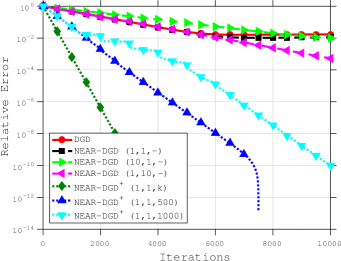
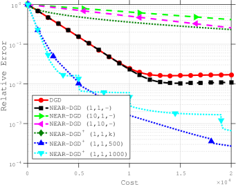
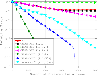
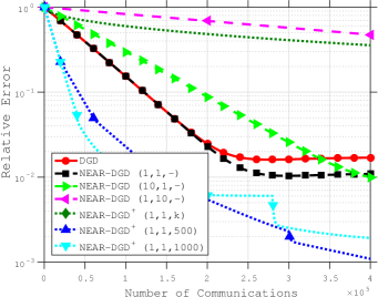
Figure 2: Performance of DGD, NEAR-DGD $(1,1,-)$, NEAR-DGD $(10,1,-)$, NEAR-DGD $(1,10,-)$, NEAR-DGD⁺ $(1,1,k)$, NEAR-DGD⁺ $(1,1,500)$, NEAR-DGD⁺ $(1,1,1000)$ measured in terms of relative error ($\|\bar{x}_{k}-x^{\star}\|^{2}/\|x^{\star}\|^{2}$) with respect to: (i) number of iterations, (ii) cost, (iii) number of gradient evaluations, and (iv) number of communications, on a quadratic problem ($n=10$, $p=10$, $\kappa=10^{4}$).

Figure 2 shows the convergence rates of the methods. As predicted by the theory, it is evident that the methods that do not increase the number of consensus steps converge only to a neighborhood of the solution, whereas methods that increase the number of consensus steps converge to the solution. We note in passing that the NEAR-DGD method (black line) converges to a better neighborhood that the DGD method (red line); this is not predicted by the theory, and is probably an artifact of the specific problem.

The NEAR-DGD⁺ method converges to the solution as predicted by the theory. In terms of number of iterations, the fastest method is the NEAR-DGD⁺ $(1,1,k)$ method. This is not surprising as the amount of work per iteration in this method is higher than that of the of NEAR-DGD⁺ $(1,1,500)$ and NEAR-DGD⁺ $(1,1,1000)$ (the practical variants). When comparing the methods in terms of the cost or the number of communications, the practical variants of the NEAR-DGD⁺ method perform significantly better. The cost metric in this case is a better indication of the performance of the method. In Figure 2 we assumed that the cost of a gradient evaluation and the cost of communication was the same, namely $c_{c}=c_{g}=1$.

In Figure 3 we show the performance of the methods for different cost structures: (i) $c_{c}=1,c_{g}=10$; (ii) $c_{c}=1,c_{g}=1$; (iii) (i) $c_{c}=10,c_{g}=1$. The cost structures where $c_{c}\neq c_{g}$ arise in applications (problems) such as those described in Section II. For example, the cost structure $c_{c}=1,c_{g}=10$ can be found in applications such as large scale machine learning problems on a cluster of physically connected computers, and the cost structure $c_{c}=10,c_{g}=1$ can be in found in applications such as controlling a swarm of battery powered robots.

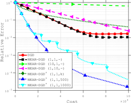
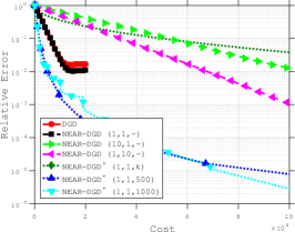
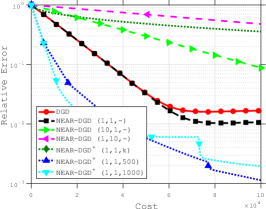
Figure 3: Performance of DGD, NEAR-DGD (1,1,-), NEAR-DGD (10,1,-), NEAR-DGD (1,10,-), NEAR-DGD⁺ (1,1,k), NEAR-DGD⁺ (1,1,500), NEAR-DGD⁺ (1,1,1000) measured in terms of relative error ($\|\bar{x}_{k}-x^{\star}\|^{2}/\|x^{\star}\|^{2}$) with respect to different cost structures, on a quadratic problem ($n=10$, $p=10$, $\kappa=10^{4}$). Left: ${\color[rgb]{0,0,0}c_{c}}=1$, ${\color[rgb]{0,0,0}c_{g}}=10$; Center: ${\color[rgb]{0,0,0}c_{c}}=1$, ${\color[rgb]{0,0,0}c_{g}}=1$; Right: ${\color[rgb]{0,0,0}c_{c}}=10$, ${\color[rgb]{0,0,0}c_{g}}=1$.

Figure 3 shows that the performance of the methods is highly dependent on the specific cost structure of the application. Although in all cases the practical variants of the NEAR-DGD⁺ method perform the best in terms of the cost, the benefit of doing multiple consensus steps varies. On the left-most figure, the benefits are very apparent, whereas on the right-most figure, the benefits are not as apparent. That being said, of course, it is still the case that the methods that do not increase the number of consensus steps cannot converge to the solution.

V-B2 Binary Classification Logistic Regression Problems

We now show numerical results illustrating the performance of the NEAR-DGD^t and NEAR-DGD⁺ methods on binary classification logistic regression problems that arise in machine learning. The objective function can be expressed as

$$f(x)=\frac{1}{n\cdot n_{i}}\sum_{i=1}^{n}\log(1+e^{-(b_{i})^{T}(A_{i}x)})+\frac{1}{n\cdot n_{i}}\|x\|_{2}^{2}$$

where $A\in\mathbb{R}^{n\cdot n_{i}\times p}$ and $b\in\{-1,1\}^{n\cdot n_{i}}$, ($n$ denotes the number of nodes, $n_{i}$ denotes the size of the local data and $p$ is the dimension of the problem) and each node $i=1,...,n$ has a portion of $A$ and $b$, $A_{i}\in\mathbb{R}^{n_{i}\times p}$ and $b_{i}\in\mathbb{R}^{n_{i}}$. We report results for the mushrooms dataset ($n=10$, $p=114$, $n_{i}=812$) [67], where the underlying graph is $4$-cyclic. Similar results were obtained for other standard machine learning datasets. For this experiment we set $c_{c}=1,c_{g}=1$.

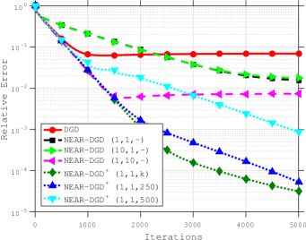
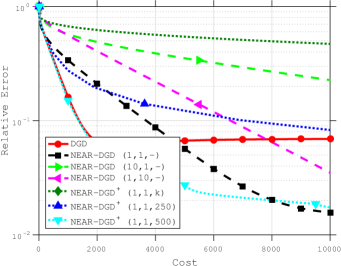
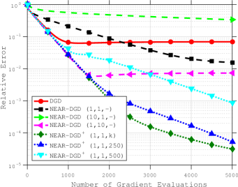
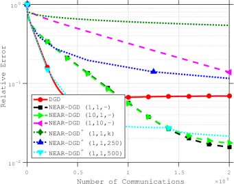
Figure 4: Performance of DGD, NEAR-DGD $(1,1,-)$, NEAR-DGD $(10,1,-)$, NEAR-DGD $(1,10,-)$, NEAR-DGD⁺ $(1,1,k)$, NEAR-DGD⁺ $(1,1,500)$, NEAR-DGD⁺ $(1,1,1000)$ measured in terms of relative error ($\|\bar{x}_{k}-x^{\star}\|^{2}/\|x^{\star}\|^{2}$) with respect to: (i) number of iterations, (ii) cost, (iii) number of gradient evaluations, and (iv) number of communications, on a binary classification logistic regression problem (mushroom. $n=10$, $p=114$, $n_{i}=812$).

Figure 4 illustrates the convergence rates of the $7$ methods. The results are similar to those for the quadratic problem. Namely, the variants that increase the number of consensus steps converge to the optimal solution whereas the other methods only converge to a neighborhood of the solution. Interestingly, the NEAR-DGD (1,1,-) method is able to converge to a significantly better neighborhood that the base DGD method. Moreover, for a fixed budget (cost), it appears that the NEAR-DGD (1,1,-) method is competitive with the NEAR-DGD⁺ variants. We should note that the figure plotting the error with respect to the cost does not show the outcome of the full experiment but rather only till the point that the DGD method terminated. However, looking at the per-iterations plots, the performance of the NEAR-DGD (1,1,-) method stagnates whereas the performance of the NEAR-DGD⁺ methods does not.

VI Final Remarks and Future Work

In this paper, we propose an adaptive cost framework to evaluate the performance of distributed optimization methods. Given a specific application, our framework incorporates the costs associated with both communication and computation in order to evaluate the efficiency of distributed optimization methods. This work is a first step towards applying the proposed general cost framework. In particular, we study the well-known distributed gradient descent (DGD) method and decompose its communication and computation steps to construct three classes of more flexible methods: DGD^t, NEAR-DGD^t and NEAR-DGD⁺.

The flexibility for each of these methods is illustrated by the fact that multiple consensus steps can be performed per gradient evaluation in environments where communication is relatively inexpensive. We show both theoretically and empirically that multiple consensus steps lead to better solution quality. We also design NEAR-DGD⁺, an exact first order method, which increases the number of consensus steps as the algorithm progresses. As such, NEAR-DGD⁺ with a constant steplength converges to the optimal solution, as opposed to the standard DGD method that only converges to a neighborhood of the optimal solution. Additionally, we show that for strongly convex functions, the NEAR-DGD⁺ method converges at a linear rate. Finally, through numerical experiments of different instances of these methods on quadratic and (binary classification) logistic regression problems, we illustrate the empirical performance of the methods and demonstrate the flexibility offered by our framework.

We should note that the same communication-computation decomposition approach can be applied seamlessly to many other distributed optimization methods, and this is a direction of future research that we wish to explore. Moreover, we plan to include other cost aspects into this framework, such as memory access, quantization and dynamic environments. Lastly, the question of how to automatically adjust the number of communication and computation steps, in an algorithmic way, depending on the environment, is a direction that we are currently investigating.

Albert S. Berahas is currently a Postdoctoral Research Fellow in the Industrial Engineering and Management Sciences (IEMS) Dept. at Northwestern University working under the supervision of Professor Jorge Nocedal. He completed his PhD studies in the Engineering Sciences and Applied Mathematics (ESAM) Dept. at Northwestern University in 2018, advised by Professor Jorge Nocedal. He received his undergraduate degree in Operations Research and Industrial Engineering (ORIE) from Cornell University in 2009, and in 2012 obtained an M.S. degree in Applied Mathematics from Northwestern University. Berahas has received the ESAM Outstanding Teaching Assistant Award, the Walter P. Murphy Fellowship and the John N. Nicholson Fellowship. Berahas’ research interests include optimization algorithms for machine learning, convex optimization and analysis, derivative-free optimization and distributed optimization.

Raghu Bollapragada is currently a PhD student in the Industrial Engineering and Management Sciences (IEMS) Dept. at Northwestern University, working under the supervision of Professor Jorge Nocedal. He received his undergraduate degree in Mechanical Engineering from Indian Institute of Technology (IIT) Madras, India in 2014. Bollapragada has received the IEMS Arthur P. Hurter Award for outstanding academic excellence among first year graduate students and the Walter P. Murphy Fellowship at Northwestern University. Bollapragada’s research interests include algorithms for machine learning, large-scale nonlinear optimization methods, convex optimization and analysis, stochastic optimization and distributed optimization.

Nitish Shirish Keskar is currently a Senior Research Scientist at Salesforce Research. He completed his PhD studies in Industrial Engineering and Management Sciences at Northwestern University in 2017. He was co-advised by Jorge Nocedal and Andreas Waechter. Prior to his PhD, Keskar received his undergraduate degree in Mechanical Engineering from VJTI in Mumbai, India. Keskar is the recipient of the 2017 best paper award for the Optimization Methods and Software journal for his paper on second-order method for L1 regularized convex optimization. Keskar’s research interests include nonlinear optimization, deep learning and large-scale computing.

Ermin Wei is currently an Assistant Professor at the EECS Dept. of Northwestern University. She completed her PhD studies in Electrical Engineering and Computer Science at MIT in 2014, advised by Professor Asu Ozdaglar, where she also obtained her M.S.. She received her undergraduate triple degree in Computer Engineering, Finance and Mathematics with a minor in German, from University of Maryland, College Park. Wei has received many awards, including the Graduate Women of Excellence Award, second place prize in Ernst A. Guillemen Thesis Award and Alpha Lambda Delta National Academic Honor Society Betty Jo Budson Fellowship. Wei’ s research interests include distributed optimization methods, convex optimization and analysis, smart grid, communication systems and energy networks and market economic analysis.

References

- [1] Q. Ling and Z. Tian, “Decentralized sparse signal recovery for compressive sleeping wireless sensor networks,” IEEE Transactions on Signal Processing, vol. 58, no. 7, pp. 3816–3827, 2010.
- [2] J. B. Predd, S. B. Kulkarni, and H. V. Poor, “Distributed learning in wireless sensor networks,” IEEE Signal Processing Magazine, vol. 23, no. 4, pp. 56–69, 2006.
- [3] I. D. Schizas, R. Ribeiro, and G. B. Giannakis, “Consensus in Ad Hoc WSNs with Noisy Links - Part I: Distributed Estimation of Deterministic Signals,” IEEE Transactions on Singal Processing, vol. 56, pp. 350–364, 2008.
- [4] F. Zhao, J. Shin, and J. Reich, “Information-driven dynamic sensor collaboration,” IEEE Signal processing magazine, vol. 19, no. 2, pp. 61–72, 2002.
- [5] Y. Cao, W. Yu, W. Ren, and G. Chen, “An overview of recent progress in the study of distributed multi-agent coordination,” IEEE Transactions on Industrial informatics, vol. 9, no. 1, pp. 427–438, 2013.
- [6] W. Ren, R. W. Beard, and E. M. Atkins, “Information consensus in multivehicle cooperative control,” IEEE Control Systems, vol. 27, no. 2, pp. 71–82, 2007.
- [7] K. Zhou and S. I. Roumeliotis, “Multirobot active target tracking with combinations of relative observations,” IEEE Transactions on Robotics, vol. 27, no. 4, pp. 678–695, 2011.
- [8] G. B. Giannakis, V. Kekatos, N. Gatsis, S. Kim, H. Zhu, and B. F. Wollenberg, “Monitoring and optimization for power grids: A signal processing perspective,” IEEE Signal Processing Magazine, vol. 30, no. 5, pp. 107–128, 2013.
- [9] V. Kekatos and G. B. Giannakis, “Distributed robust power system state estimation,” IEEE Transactions on Power Systems, vol. 28, no. 2, pp. 1617–1626, 2013.
- [10] J. C. Duchi, A. Agarwal, and M. J. Wainwright, “Dual Averaging for Distributed Optimization: Convergence Analysis and Network Scaling,” IEEE Transactions on Automatic Control, vol. 57, no. 3, pp. 592–606, 2012.
- [11] K. Tsianos, S. Lawlor, and M. G. Rabbat, “Consensus-based distributed optimization: Practical issues and applications in large-scale machine learning,” in Communication, Control, and Computing (Allerton), 2012 50th Annual Allerton Conference on. IEEE, 2012, pp. 1543–1550.
- [12] D. P. Bertsekas and J. N. Tsitsiklis, Parallel and distributed computation: numerical methods. Prentice hall Englewood Cliffs, NJ, 1989, vol. 23.
- [13] A. Nedić and A. Ozdaglar, “Distributed subgradient methods for multi-agent optimization,” IEEE Transactions on Automatic Control, vol. 54, no. 1, pp. 48–61, 2009.
- [14] J. N. Tsitsiklis, “Problems in Decentralized Decision Making and Computation,” Ph.D. dissertation, Dept. of Electrical Engineering and Computer Science, Massachusetts Institute of Technology, 1984.
- [15] S. Boyd, A. Ghosh, B. Prabhakar, and D. Shah, “Randomized gossip algorithms,” IEEE/ACM Transactions on Networking (TON), vol. 14, no. SI, pp. 2508–2530, 2006.
- [16] A. Jadbabaie, J. Lin, and S. Morse, “Coordination of Groups of Mobile Autonomous Agents using Nearest Neighbor Rules,” IEEE Transactions on Automatic Control, vol. 48, no. 6, pp. 988–1001, 2003.
- [17] D. Jakovetic, J. Xavier, and J. M. F. Moura, “Fast Distributed Gradient Methods,” IEEE Transactions on Automatic Control, vol. 59, no. 5, pp. 1131–1146, 2014.
- [18] B. Johansson, T. Keviczky, M. Johansson, and K. H. Johansson, “Subgradient Methods and Consensus Algorithms for Solving Convex Optimization Problems,” Proceedings of IEEE Conference on Decision and Control(CDC), pp. 4185–4190, 2008.
- [19] I. Lobel and A. Ozdaglar, “Convergence Analysis of Distributed Subgradient Methods over Random Networks,” Proceedings of Annual Allerton Conference on Communication, Control, and Computing, 2008.
- [20] I. Lobel, A. Ozdaglar, and D. Feijer, “Distributed Multi-agent Optimization with State-Dependent Communication,” Mathematical Programming, special issue in honor of Paul Tseng, vol. 129, no. 2, pp. 255–284, 2011.
- [21] I. Matei and J. S. Baras, “Performance Evaluation of the Consensus-Based Distributed Subgradient Method Under Random Communication Topologies,” IEEE Journal of Selected Topics in Signal Processing, vol. 5, no. 4, pp. 754–771, 2011.
- [22] A. Nedić, “Asynchronous broadcast-based convex optimization over a network,” IEEE Transactions on Automatic Control, vol. 56, no. 6, pp. 1337–1351, 2011.
- [23] A. Nedić, A. Olshevsky, A. Ozdaglar, and J. N. Tsitsiklis, “Distributed Subgradient Algorithms and Quantization Effects,” Proceedings of IEEE Conference on Decision and Control (CDC), 2008.
- [24] A. Nedić and A. Ozdaglar, Convex Optimization in Signal Processing and Communications. Eds., Eldar, Y. and Palomar, D., Cambridge University Press, 2008, ch. Cooperative distributed multi-agent optimization.
- [25] ——, “Approximate primal solutions and rate analysis for dual subgradient methods,” SIAM Journal on Optimization, vol. 19(4), pp. 1757–1780, 2009.
- [26] A. Nedić, A. Ozdaglar, and P. A. Parrilo, “Constrained Consensus and Optimization in Multi-agent Networks,” IEEE Transactions on Automatic Control, vol. 55(4), pp. 922–938, 2010.
- [27] S. S. Ram, A. Nedić, and V. V. Veeravalli, “Distributed Stochastic Subgradient Projection Algorithms for Convex Optimization,” Journal of Optimization Theory and Applications, vol. 147, no. 3, pp. 516–545, 2010.
- [28] S. S. Ram, A. Nedić, and V. V. Veeravalli, “Asynchronous gossip algorithm for stochastic optimization: Constant stepsize analysis,” in Recent Advances in Optimization and its Applications in Engineering. Springer, 2010, pp. 51–60.
- [29] W. Shi, Q. Ling, G. Wu, and W. Yin, “Extra: An exact first-order algorithm for decentralized consensus optimization,” SIAM Journal on Optimization, vol. 25, no. 2, pp. 944–966, 2015.
- [30] K. Srivastava and A. Nedić, “Distributed asynchronous constrained stochastic optimization,” IEEE Journal of Selected Topics in Signal Processing, vol. 5, no. 4, pp. 772–790, 2011.
- [31] M. Hong, M. Razaviyayn, Z. Luo, and J. Pang, “A unified algorithmic framework for block-structured optimization involving big data: With applications in machine learning and signal processing,” IEEE Signal Processing Magazine, vol. 33, no. 1, pp. 57–77, 2016.
- [32] Z. Peng, Y. Xu, M. Yan, and W. Yin, “Arock: an algorithmic framework for asynchronous parallel coordinate updates,” SIAM Journal on Scientific Computing, vol. 38, no. 5, pp. A2851–A2879, 2016.
- [33] P. Richtárik and M. Takáč, “Parallel coordinate descent methods for big data optimization,” Mathematical Programming, vol. 156, no. 1-2, pp. 433–484, 2016.
- [34] Y. Nesterov, “Primal-dual subgradient methods for convex problems,” Mathematical Programming, vol. 120, no. 1, pp. 221–259, 2009.
- [35] D. P. Bertsekas, “Incremental Gradient, Subgradient, and Proximal Methods for Convex Optimization: A Survey,” LIDS Report 2848, 2010.
- [36] S. Boyd, N. Parikh, E. Chu, B. Peleato, and J. Eckstein, “Distributed Optimization and Statistical Learning via the Alternating Direction Method of Multipliers,” Foundations and Trends in Machine Learning, vol. 3, no. 1, pp. 1–122, 2010.
- [37] T. Chang, M. Hong, W. Liao, and X. Wang, “Asynchronous Distributed ADMM for Large-Scale Optimization—Part I: Algorithm and Convergence Analysis,” IEEE Transactions on Signal Processing, vol. 64, no. 12, pp. 3118–3130, 2015.
- [38] J. Eckstein, “Augmented Lagrangian and Alternating Direction Methods for Convex Optimization: A Tutorial and Some Illustrative Computational Results,” Rutcor Research Report, 2012.
- [39] P. Giselsson and S. Boyd, “Diagonal scaling in douglas-rachford splitting and admm,” in Decision and Control (CDC), 2014 IEEE 53rd Annual Conference on. IEEE, 2014, pp. 5033–5039.
- [40] F. Iutzeler, P. Bianchi, P. Ciblat, and W. Hachem, “Asynchronous Distributed Optimization using a Randomized Alternating Direction Method of Multipliers,” Submitted to IEEE Conference on Decision and Control (CDC), 2013.
- [41] J. Mota, J. Xavier, P. Aguiar, and M. Püschel, “ADMM For Consensus On Colored Networks,” Proceedings of IEEE Conference on Decision and Control (CDC), 2012.
- [42] ——, “D-ADMM : A Communication-Efficient Distributed Algorithm For Separable Optimization,” IEEE Transactions on Signal Processing, vol. 61, no. 10, pp. 2718–2723, 2013.
- [43] E. Wei and A. Ozdaglar, “Distributed Alternating Direction Method of Multipliers,” Proceedings of IEEE Conference on Decision and Control (CDC), 2012.
- [44] ——, “On the convergence of asynchronous distributed alternating Direction Method of Multipliers,” in Global Conference on Signal and Information Processing (GlobalSIP), 2013 IEEE. IEEE, 2013, pp. 551–554.
- [45] L. Xiao and T. Zhang, “A proximal stochastic gradient method with progressive variance reduction,” SIAM Journal on Optimization, vol. 24, no. 4, pp. 2057–2075, 2014.
- [46] H. Zhu, A. Cano, and G. B. Giannakis, “In-Network Channel Decoding Using Consensus on Log-Likelihood Ratio Averages,” Proceedings of Conference on Information Sciences and Systems (CISS), 2008.
- [47] M. Eisen, A. Mokhtari, and A. Ribeiro, “Decentralized quasi-newton methods,” IEEE Transactions on Signal Processing, vol. 65, no. 10, pp. 2613–2628, 2017.
- [48] F. Mansoori and E. Wei, “Superlinearly Convergent Asynchronous Distributed Network Newton Method,” Proceedings of IEEE Conference on Decision and Control (CDC), 2017.
- [49] A. Mokhtari, Q. Ling, and A. Ribeiro, “Network newton-part i: Algorithm and convergence,” arXiv preprint arXiv:1504.06017, 2015.
- [50] ——, “Network newton-part ii: Convergence rate and implementation,” arXiv preprint arXiv:1504.06020, 2015.
- [51] Y. Chow, W. Shi, T. Wu, and W. Yin, “Expander graph and communication-efficient decentralized optimization,” in Signals, Systems and Computers, 2016 50th Asilomar Conference on. IEEE, 2016, pp. 1715–1720.
- [52] G. Lan, S. Lee, and Y. Zhou, “Communication-efficient algorithms for decentralized and stochastic optimization,” arXiv preprint arXiv:1701.03961, 2017.
- [53] O. Shamir, N. Srebro, and T. Zhang, “Communication-efficient distributed optimization using an approximate newton-type method,” in International conference on machine learning, 2014, pp. 1000–1008.
- [54] K. Tsianos, S. Lawlor, and M. G. Rabbat, “Communication/computation tradeoffs in consensus-based distributed optimization,” in Advances in neural information processing systems, 2012, pp. 1943–1951.
- [55] Y. Zhang and X. Lin, “Disco: Distributed optimization for self-concordant empirical loss,” in International conference on machine learning, 2015, pp. 362–370.
- [56] Y. Zhang, M. J. Wainwright, and J. C. Duchi, “Communication-efficient algorithms for statistical optimization,” in Advances in Neural Information Processing Systems, 2012, pp. 1502–1510.
- [57] A. H. Sayed, Diffusion adaptation over networks. Academic Press Library in Signal Processing, 2013, vol. 3.
- [58] A. I. Chen and A. Ozdaglar, “A fast distributed proximal-gradient method,” in Communication, Control, and Computing (Allerton), 2012 50th Annual Allerton Conference on. IEEE, 2012, pp. 601–608.
- [59] P. Di Lorenzo and G. Scutari, “Next: In-network nonconvex optimization,” IEEE Transactions on Signal and Information Processing over Networks, vol. 2, no. 2, pp. 120–136, 2016.
- [60] A. Nedić, A. Olshevsky, and W. Shi, “Achieving geometric convergence for distributed optimization over time-varying graphs,” arXiv preprint arXiv:1607.03218, 2016.
- [61] G. Qu and N. Li, “Harnessing smoothness to accelerate distributed optimization,” IEEE Transactions on Control of Network Systems, 2017.
- [62] Z. Li, W. Shi, and M. Yan, “A decentralized proximal-gradient method with network independent step-sizes and separated convergence rates,” arXiv preprint arXiv:1704.07807, 2017.
- [63] K. Yuan, Q. Ling, and W. Yin, “On the convergence of decentralized gradient descent,” SIAM Journal on Optimization, vol. 26, no. 3, pp. 1835–1854, 2016.
- [64] A. S. Berahas, R. Bollapragada, N. S. Keskar, and E. Wei, “Balancing communication and computation in distribution optimization,” arXiv preprint arXiv:1709.02999, 2017.
- [65] A. Mokhtari, Q. Ling, and A. Ribeiro, “Network newton distributed optimization methods,” IEEE Transactions on Signal Processing, vol. 65, no. 1, pp. 146–161, 2017.
- [66] Y. Nesterov, Introductory lectures on convex optimization: A basic course. Springer Science & Business Media, 2013, vol. 87.
- [67] C. C. Chang and C. J. Lin, “Libsvm: a library for support vector machines,” ACM transactions on intelligent systems and technology (TIST), vol. 2, no. 3, p. 27, 2011.