A Smooth Constant-Roll to a Slow-Roll Modular Inflation Transition

Abstract

In this work, we investigate how a smooth transition from a constant-roll to a slow-roll inflationary era may be realized, in the context of a canonical scalar field theory. We study in some detail the dynamical evolution of the cosmological system, and we investigate whether a stable attractor exists, both numerically and analytically. We also investigate the slow-roll era and as we demonstrate, partially compatibility of the resulting scalar theory, may be achieved, with the potential of the latter belonging to a class of modular inflationary potentials. The novel features of the constant-roll to slow-roll transition which we achieved, are firstly that the it is not compelling for the slow-roll era to last for $N\sim 50-60$ $e$-foldings, but it may last for a smaller number of $e$-foldings, since some $e$-foldings may occur during the constant-roll era. Secondly, when the slow-roll era occurs after the constant-roll era, the graceful exit from inflation may occur, a feature absent in the constant-roll scenario, due to the stability properties of the final attractor in the constant-roll case.

I Introduction

The inflationary era is unarguably one of the successes of modern theoretical physics, and in the literature there exist various approaches, see Refs. inflation1 ; inflation2 ; inflation3 ; inflation4 ; inflation5 for some reviews, and also Refs. Nojiri:2006ri ; Capozziello:2011et ; Capozziello:2010zz ; Nojiri:2010wj ; Clifton:2011jh ; Nojiri:2017ncd for modified gravity descriptions of the inflationary era. The first approach, and quite common, uses a slow-rolling canonical scalar field inflation1 ; inflation2 , and recently the observational data coming from Planck planck , indicated that plateau-like potentials are preferred. Although some single scalar field models of inflation are observationally viable, the single scalar field description of inflation, leaves no room for non-Gaussianities in the power spectrum. Up to date, the various distinct modes of the primordial curvature perturbations are assumed to be uncorrelated, which yields the Gaussian property of the power spectrum. The Gaussian property of the primordial modes is up to date supported by the observational data, however, if non-Gaussianities are detected in the future, this will put the single scalar field of inflation models in question. For a recent review on non-Gaussianities, see Ref. Chen:2010xka .

A solution to this issue for single scalar field models, is to modify the slow-roll condition, and allow a constant-roll era for the canonical scalar field Inoue:2001zt ; Tsamis:2003px ; Kinney:2005vj ; Namjoo:2012aa ; Martin:2012pe ; Motohashi:2014ppa ; Cai:2016ngx ; Hirano:2016gmv ; Cook:2015hma ; Anguelova:2015dgt ; Kumar:2015mfa ; Odintsov:2017yud ; Odintsov:2017qpp ; Nojiri:2017qvx ; Fei:2017fub ; Gao:2017owg . In some previous works Odintsov:2017yud ; Odintsov:2017qpp we demonstrated that it is possible to combine a constant-roll with a slow-roll era, and achieve a smooth transition between these eras. Particularly in Ref. Odintsov:2017yud we showed that it is possible to achieve a smooth transition between a slow-roll era at early times, and a constant-roll era at the latest stages of the inflationary era. Also in Ref. Odintsov:2017qpp we demonstrated that it is possible to achieve a transition between to constant-roll eras. However, in both cases, the inflationary era ends up to a constant-roll cosmological attractor, so it was not possible to end this inflationary era, since the attractor was stable. To this end, in this paper we shall demonstrate how to achieve a transition between a constant-roll era, which occurs at the early stages of the inflationary era, and a slow-roll era, which occurs at the late stages of the inflationary era. The interesting features of this approach is that firstly the slow-roll era is not required to last for $N\sim 50-60$ $e$-foldings, but possibly lasts for a smaller number of $e$-foldings, since some $e$-foldings may occur during the constant-roll era. Secondly, with the slow-roll era occurring after the slow-roll era, one may obtain an inflationary model which is compatible with the Planck planck data, but also the graceful exit from inflation is possible. As we will demonstrate, the model we shall present can have compatibility with the Planck data, however we could not achieve simultaneous compatibility of both the spectral index and the scalar-to-tensor ratio. Interestingly enough, the resulting slow-roll model has a potential that belongs to a class of modified modular inflation BenDayan:2008dv .

This paper is organized as follows: In section II, we shall briefly present the essential features of the transition mechanism between constant and slow-roll eras, and also we discuss several issues regarding the cosmological dynamics. In section III, we shall present the model of transition from a constant to slow-roll era, and we shall study the dynamical properties of the cosmological system. We investigate if the dynamical solution we obtain can drive the transition ,and we validate if this solution is the final attractor, both numerically and analytically. Finally, we calculate the observational indices and we examine the parameter space in order to see when compatibility with the observational data may be achieved. Finally, the conclusions follow in the end of the paper.

Before we start, we need to clarify the choice of the geometric background which we will adopt in the rest of this paper. The geometric background is assumed to be a flat Friedmann-Robertson-Walker metric with line element,

$$ds^{2}=-dt^{2}+a(t)^{2}\sum_{i=1,2,3}\left(dx^{i}\right)^{2}\,,$$ (1)

with $a(t)$ being the scale factor. Also, the connection is assumed to be a metric compatible, symmetric and torsion-less affine connection, the Levi-Civita connection.

II Essential Features of Dynamical Transitions Between Constant-Roll Inflation and Slow-Roll Inflation

In order to maintain the article self-contained, we shall briefly present the formalism we developed in our previous works Odintsov:2017yud ; Odintsov:2017qpp . We shall consider a canonical scalar field theory, with the geometric background being a flat FRW one, with the scalar action being,

$$\mathcal{S}=\sqrt{-g}\left(\frac{R}{2}-\frac{1}{2}\partial_{\mu}\phi\partial^{\mu}\phi-V(\varphi))\right)\,,$$ (2)

where $V(\varphi)$ is the canonical scalar potential. The corresponding scalar energy density is equal to,

$$\rho=\frac{1}{2}\dot{\varphi}^{2}+V(\varphi)\,,$$ (3)

and in addition, the corresponding pressure is,

$$P=\frac{1}{2}\dot{\varphi}^{2}-V(\varphi)\,.$$ (4)

In effect, the Friedmann equation is,

$$H^{2}=\frac{1}{3M_{p}^{2}}\rho\,,$$ (5)

and it is easy to show that,

$$\dot{H}=-\frac{1}{2M_{p}^{2}}\dot{\varphi}^{2}\,.$$ (6)

Moreover, the canonical scalar field obeys the Klein-Gordon equation,

$$\ddot{\varphi}+3H\dot{\varphi}+V^{\prime}=0\,,$$ (7)

where the prime denotes differentiation with respect to $\varphi$.

In most inflationary theories, the inflationary dynamical evolution is determined by the slow-roll parameters, and for the scalar theory these are $\epsilon$ and $\eta$, which are actually the leading order terms in the perturbative expansion known as Hubble slow-roll expansion Liddle:1994dx . The slow-roll parameters $\epsilon$ and $\eta$ are defined as follows,

$$\epsilon=-\frac{\dot{H}}{H^{2}}\,,\quad\eta=-\frac{\ddot{H}}{2H\dot{H}}\,,$$ (8)

and also these can be written in terms of the canonical scalar field as follows,

$$\epsilon=\frac{\dot{\varphi}^{2}}{2M_{p}^{2}H^{2}}\,,\quad\eta=-\frac{\ddot{\varphi}}{2H\dot{\varphi}}\,.$$ (9)

Recently, the slow-roll theoretical framework was extended, and in the new framework known as constant-roll inflation Martin:2012pe ; Motohashi:2014ppa , the second slow-roll index $\eta$, may become a constant number $\eta=-n$, which is not required to be small in magnitude Martin:2012pe . The constant-roll inflationary framework was further extended in Refs. Odintsov:2017yud ; Odintsov:2017qpp , in which, transition between constant and slow-roll eras are possible. This framework is based on the basic assumption that the second slow-roll index $\eta$ has the following form,

$$\eta=-f(\varphi(t))\,,$$ (10)

which can be written as follows,

$$\frac{\ddot{\varphi}}{2H\dot{\varphi}}=f(\varphi(t))\,,$$ (11)

where function $f(\varphi(t))$ in Eqs. (10) and (11) is considered to be a smooth and monotonic function of $\varphi(t)$, and also it has to be dimensionless. Also the functional behavior will determine the transition between constant and slow roll eras.

As in our previous works we shall use the Hamilton-Jacobi formalism, and our aim is to find the Hubble rate expressed in terms of the canonical scalar $H(\varphi)$, by solving the corresponding equations of motion. An important aim is to check whether the solution $H(\varphi)$ is the final attractor of the cosmological dynamical system, regardless of the choice of the initial conditions, and we will check this both analytically and numerically in the next section. Let us present in brief some of the basic equations of the cosmological dynamical system we shall use. Due to the fact that,

$$\dot{H}=\dot{\varphi}\frac{\mathrm{d}H}{\mathrm{d}\varphi}\,,$$ (12)

Eq. (6) can be cast as follows,

$$\dot{\varphi}=-2M_{p}^{2}\frac{\mathrm{d}H}{\mathrm{d}\varphi}\,,$$ (13)

and by combining Eqs. (13) and (11), after some algebra we obtain the following,

$$\frac{\mathrm{d}^{2}H}{\mathrm{d}\varphi^{2}}=-\frac{1}{2M_{p}^{2}}f(\varphi)H(\varphi)\,.$$ (14)

The differential equation (14) is of central importance in this paper, since this will determine the function $H(\varphi)$, which may or may not be the final attractor of the cosmological dynamical system. Having the function $H(\varphi)$ at hand, the scalar potential can easily be found by combining Eqs. (13) and (5), and it reads,

$$V(\varphi)=3M_{p}^{2}H(\varphi)^{2}-2M_{p}^{4}(H^{\prime}(\varphi))^{2}\,.$$ (15)

In the next section, we shall use the formalism we developed in this paper, and as we will show, we shall achieve a smooth transition from a constant to a slow-roll era.

III A Smooth Transition from a Constant-roll era to a Slow-roll Era

The choice of the function $f(\varphi(t))$ plays a crucial role in order for the transitions to occur, and it is conceivable to notice that during the constant-roll era, the function $f(\varphi(t)$ must be a constant, and during the slow-roll era, it has to be approximately $f(\varphi(t))\simeq 0$. In order to achieve a transition from a constant-roll era to a slow-roll era, we shall assume that the function $f(\varphi(t))$ appearing in Eq. (11), has the following form,

$$f(\varphi(t))=\frac{\alpha\sinh(\lambda x)}{\gamma+\alpha\sinh(\lambda x)}\,,$$ (16)

where for the purposes of this work $\lambda$ is assumed to be equal to $\lambda=\frac{\sqrt{\frac{1}{2}}}{M_{p}}$, and the parameters $\gamma$ and $\alpha$ are dimensionless parameters. The choice of $f(\varphi(t)$ appearing in Eq. (16) dictates that the constant-roll era occurs for large field values, when $\frac{\varphi}{M_{p}}\gg 1$, and as the field values decrease, when $\varphi<M_{p}$ the slow-roll era commences. Hence, the slow-roll era which we will discuss in this paper, belongs to the small field inflationary models. For large field values, the function $f(\varphi(t))$ behaves as, $f(\varphi\gg M_{p})\sim 1$, while for small field values, it behaves as $f(\varphi\ll M_{p})\sim 0$, so for small field values a slow-roll era is realized. Hence, the constant-roll era corresponds to the scenario studied in Ref. Motohashi:2014ppa , with $\alpha=-4$, if we use the notation of Ref. Motohashi:2014ppa .

Let us now proceed by finding the solution of the differential equation (14), with the function $f(\varphi(t))$ being chosen as in Eq. (16), and the resulting solution for $H(\varphi)$ is,

$$H(\varphi)=\gamma+\alpha\sinh\left(\frac{\varphi}{2M_{p}^{2}}\right)\,.$$ (17)

Accordingly, the scalar potential $V(\varphi)$ can be found, by combining Eqs. (17) and (15), and it is equal to,

$$V(\varphi)=M_{p}^{2}\left(-2\alpha^{2}+3\gamma^{2}+\alpha^{2}\cosh\left(\frac{\sqrt{2}\varphi}{M_{p}}\right)+6\alpha\gamma\sinh\left(\frac{\varphi}{\sqrt{2}M_{p}}\right)\right)\,.$$ (18)

The potential can be further simplified for small field values, so during the slow-roll era of the scalar field $\varphi$, and the simplified potential reads,

$$V(\varphi)\simeq 3\gamma^{2}M_{p}^{2}-\alpha^{2}M_{p}^{2}\cosh^{2}\left(\frac{\varphi}{\sqrt{2}M_{p}}\right)\,,$$ (19)

and by further expanding the second term in powers of the scalar field, in the small $\varphi/M_{p}$ limit, we obtain,

$$V(\varphi)\simeq-\frac{\alpha^{2}\varphi^{2}}{2}+3\gamma^{2}M_{p}^{2}-\frac{\alpha^{2}\varphi^{4}}{12M_{p}^{2}}-\alpha^{2}M_{p}^{2}\,.$$ (20)

The potential (20) is a type of modular inflationary potential, which can be found in Ref. BenDayan:2008dv , and the general form of the potential is,

$$V(\varphi)=\alpha_{1}-\alpha_{2}\varphi^{2}-\alpha_{3}\varphi^{q}\,.$$ (21)

Obviously, the potential (20) corresponds to the case $q=4$ of the potential (21). As we show later on this section, the potential (20) leads to an interesting phenomenology, partially compatible with the 2015 Planck data planck . Before getting to that, we need to investigate whether the solution $H(\varphi)$ is the final attractor of the cosmological dynamical system, so we will check this both numerically and analytically. We start off with the numerical approach, so we choose the following values for the parameters $\alpha$ and $\gamma$ (the reasons for this choice will become clear later on),

$$\alpha=0.165,\,\,\,\gamma=2\,,$$ (22)

and also recall that $\lambda=\frac{\sqrt{\frac{1}{2}}}{M_{p}}$. For the values of the parameters chosen as in (22), in Fig. 1 we present the phase space diagram $\dot{\varphi}-\varphi$ corresponding to the solution (17), by using the initial conditions $\varphi(0)=10^{20}$ (blue curve) and $\varphi(0)=10^{19}$ (red curve).

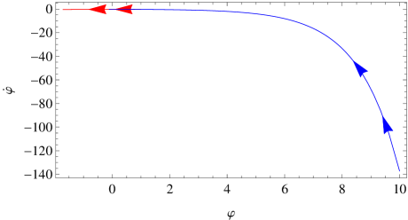
Figure 1: The phase space diagram of the solution (17), for the initial conditions $\varphi(0)=10^{20}$ (blue curve) and $\varphi(0)=10^{19}$ (red curve).

It is obvious from Fig. (1), that the solution (17) is the final attractor of the cosmological dynamical system, since an attractor behavior occurs, regardless the choice of initial conditions. We need to note that the final attractor has appealing physical properties, since at the field values decrease, the velocity of the field $\dot{\varphi}$ also decreases.

Apart from the above numerical study for the stability of the attractor, we can also investigate it’s stability analytically. We shall adopt the technique developed in Ref. Liddle:1994dx , so we vary Eq. (15), and we get the following differential equation with respect to $\delta H(\varphi)$,

$$H_{0}^{\prime}(\varphi)\delta H^{\prime}(\varphi)\simeq\frac{3}{2M_{p}^{2}}H_{0}(\varphi)\delta H(\varphi)\,,$$ (23)

where $H_{0}(varphi)$ is the solution (17). The general solution of the differential equation (23) is,

$$\delta H(\varphi)=\delta H(\varphi_{0})e^{\frac{3}{2M_{p}^{2}}\int_{\varphi_{0}}^{\varphi}\frac{H_{0}(\varphi)}{H_{0}(\varphi)}}\,,$$ (24)

where the parameter $\varphi_{0}$ denotes some initial value of $\varphi$. Then, having the solution $H_{0}(\varphi)$ at hand, we can investigate whether this solution is a stable final attractor of the cosmological system, by studying the evolution of the linear perturbations (24) as a function of $\varphi$. Clearly, if the perturbations grow, the solution $H_{0}(\varphi)$ s unstable, and on the contrary case, it proves to be stable, at list at a linear perturbation theory context. The sign of the exponential term in (24), determines whether the perturbations grow (positive sign), or decay (negative sign). In Fig. 2 we present the behavior of the terms appearing in the exponential terms, as a function of $\varphi$.

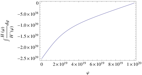
Figure 2: Stability of linear perturbations for the solution $H(\varphi)=\gamma+\alpha\sinh\left(\frac{\varphi}{2M_{p}^{2}}\right)$.

As it can be seen, the term in the exponent is negative, hence the perturbations decay, and therefore the solution (17) is stable towards linear perturbations, and thus it is the final attractor of the theory.

Having discussed the attractor properties of the solution (17), let us now focus on the slow-roll era, and we examine the viability of the canonical scalar field model (20), by confronting the corresponding observational indices with the 2015 Planck data planck . The potential in the limit $\varphi<M_{p}$ is given in Eq. (20), so by using this we will calculate the slow-roll indices $\epsilon$ and $\eta$, which in terms of the potential in the context of the slow-roll approximation, can be written as follows,

$$\epsilon(\varphi)=\frac{M_{p}^{2}}{2}\left(\frac{V^{\prime}(\varphi)}{V(\varphi)}\right)^{2},\,\,\,\eta(\varphi)=M_{p}^{2}\frac{V^{\prime\prime}(\varphi)}{V(\varphi)}\,.$$ (25)

Having $\epsilon$ and $\eta$ at hand, we can calculate the corresponding observational indices, namely the spectral index of the primordial curvature perturbations and the scalar-to-tensor ratio. The latter two in the case of a canonical scalar field, can be written in the following form,

$$n_{s}\simeq 1-6\epsilon+2\eta,\,\,\,r=16\epsilon\,.$$ (26)

By using the definition of the $e$-foldings number,

$$N\simeq\frac{1}{M_{p}^{2}}\int_{\varphi_{f}}^{\varphi_{i}}\frac{V(\varphi)}{V^{\prime}(\varphi)}\mathrm{d}\varphi\,,$$ (27)

where $\varphi_{i}$ is the value of the scalar field at the horizon crossing, and also by determining the final value of the scalar field when $\epsilon\sim 1$, we can obtain, after some extensive algebra, the spectral index $n_{s}$, which at leading order is,

$$n_{s}\simeq\frac{2\alpha^{2}M_{p}^{2}\left(\left(-\frac{6\gamma^{2}}{\alpha^{2}}+\frac{\sqrt{3}\mathcal{Q}(\alpha,\gamma)}{\alpha^{4}M_{p}^{2}}+1\right)e^{\frac{2\alpha^{2}N}{\alpha^{2}-3\gamma^{2}}}-1\right)}{\alpha^{2}\left(-M_{p}^{2}\right)+3\gamma^{2}M_{p}^{2}+\frac{\left(\sqrt{3}\mathcal{Q}(\alpha,\gamma)+M_{p}^{2}\left(\alpha^{4}-6\alpha^{2}\gamma^{2}\right)\right)e^{\frac{2\alpha^{2}N}{\alpha^{2}-3\gamma^{2}}}}{2\alpha^{2}}-\frac{\left(\sqrt{3}\mathcal{Q}(\alpha,\gamma)+M_{p}^{2}\left(\alpha^{4}-6\alpha^{2}\gamma^{2}\right)\right)^{2}e^{\frac{4\alpha^{2}N}{\alpha^{2}-3\gamma^{2}}}}{12\alpha^{6}M_{p}^{2}}}+1$$ (28)

$$\frac{48\alpha^{4}M_{p}^{2}\left(M_{p}^{2}\left(\frac{6\gamma^{2}}{\alpha^{2}}-1\right)-\frac{\sqrt{3}\mathcal{Q}(\alpha,\gamma)}{\alpha^{4}}\right)e^{\frac{2\alpha^{2}N}{\alpha^{2}-3\gamma^{2}}}\left(3M_{p}^{2}+\left(M_{p}^{2}\left(\frac{6\gamma^{2}}{\alpha^{2}}-1\right)-\frac{\sqrt{3}\mathcal{Q}(\alpha,\gamma)}{\alpha^{4}}\right)e^{\frac{2\alpha^{2}N}{\alpha^{2}-3\gamma^{2}}}\right)^{2}}{\left(\alpha^{2}\left(12M_{p}^{4}+6M_{p}^{2}\left(M_{p}^{2}\left(\frac{6\gamma^{2}}{\alpha^{2}}-1\right)-\frac{\sqrt{3}\mathcal{Q}(\alpha,\gamma)}{\alpha^{4}}\right)e^{\frac{2\alpha^{2}N}{\alpha^{2}-3\gamma^{2}}}+\frac{\left(\sqrt{3}\mathcal{Q}(\alpha,\gamma)+M_{p}^{2}\left(\alpha^{4}-6\alpha^{2}\gamma^{2}\right)\right)^{2}e^{\frac{4\alpha^{2}N}{\alpha^{2}-3\gamma^{2}}}}{\alpha^{8}}\right)-36\gamma^{2}M_{p}^{4}\right)^{2}}$$

where $\mathcal{Q}(\alpha,\gamma)$ stands for,

$$\mathcal{Q}(\alpha,\gamma)=\sqrt{\alpha^{6}\left(-M_{p}^{4}\right)\left(\alpha^{2}-4\gamma^{2}\right)}\,.$$ (29)

Accordingly, the scalar-to-tensor ration can be found, and it’s analytic expression at leading order is,

$$r\simeq\frac{128\alpha^{4}M_{p}^{2}\left(M_{p}^{2}\left(\frac{6\gamma^{2}}{\alpha^{2}}-1\right)-\frac{\sqrt{3}\mathcal{Q}(\alpha,\gamma)}{\alpha^{4}}\right)e^{\frac{2\alpha^{2}N}{\alpha^{2}-3\gamma^{2}}}\left(3M_{p}^{2}+\left(M_{p}^{2}\left(\frac{6\gamma^{2}}{\alpha^{2}}-1\right)-\frac{\sqrt{3}\mathcal{Q}(\alpha,\gamma)}{\alpha^{4}}\right)e^{\frac{2\alpha^{2}N}{\alpha^{2}-3\gamma^{2}}}\right)^{2}}{\left(\alpha^{2}\left(12M_{p}^{4}+6M_{p}^{2}\left(M_{p}^{2}\left(\frac{6\gamma^{2}}{\alpha^{2}}-1\right)-\frac{\sqrt{3}\mathcal{Q}(\alpha,\gamma)}{\alpha^{4}}\right)e^{\frac{2\alpha^{2}N}{\alpha^{2}-3\gamma^{2}}}+\frac{\left(\sqrt{3}\mathcal{Q}(\alpha,\gamma)+M_{p}^{2}\left(\alpha^{4}-6\alpha^{2}\gamma^{2}\right)\right)^{2}e^{\frac{4\alpha^{2}N}{\alpha^{2}-3\gamma^{2}}}}{\alpha^{8}}\right)-36\gamma^{2}M_{p}^{4}\right)^{2}}$$ (30)

The 2015 Planck data planck constrain the observational indices as follows,

$$n_{s}=0.9644\pm 0.0049\,,\quad r<0.10\,,$$ (31)

so now we will investigate the parameter space to see if the compatibility with the Planck data can be achieved. After thoroughly analyzing the parameter space, the resulting picture is that compatibility with the Planck data can be obtained for a large range of the parameters separately for the spectral index and the scalar-to-tensor ratio, but not together. For example by choosing $\gamma=2$ and $\alpha=0.165$, we get $n_{s}=0.964898$ and $r=0.185485$, so the scalar-to-tensor ratio is excluded. This picture seems to persist regardless on the magnitude of the free parameters. In Fig. 3, we plot the spectral index as a function of $\alpha$ for $\gamma=2$, and for $N=60$ (black and dashed curve) and $N=40$ (blue curve). The upper red dashed line is the upper limit of the Planck allowed value for the spectral index, $n_{s}=0.9693$ and the lower red and dashed line, the lower Planck compatible limit on $n_{s}$, namely $n_{s}=0.9595$.

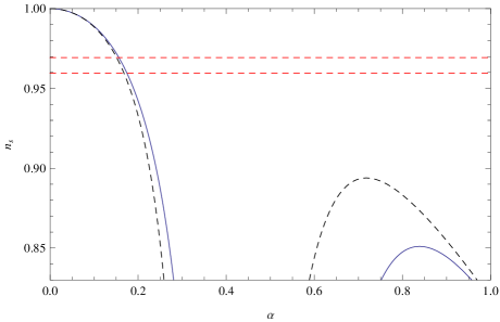
Figure 3: The spectral index as a function of $\alpha$ for $\gamma=2$, and for $N=60$ (black and dashed curve) and $N=40$ (blue curve). The upper red dashed line is the upper limit of the Planck allowed value for the spectral index, $n_{s}=0.9693$ and the lower red and dashed line, the lower Planck compatible limit on $n_{s}$, namely $n_{s}=0.9595$.

As it can be seen in Fig 3, the compatibility with the Planck data can be achieved even for $N<50$. This is the new feature of the present paper, since it is possible to obtain a viable spectral index inflationary theory, with $N<50$ during the slow-roll era, since some $e$-foldings may occur during the constant-roll era. The drawback is that the spectral index and the scalar-to-tensor ratio are not simultaneously compatible with the Planck data. For completeness, in Fig. 4, we plot the behavior of the scalar-to-tensor ratio as a function of the parameter $\alpha$, for $\gamma=2$, and for $N=60$ (black and dashed curve) and $N=40$ (blue curve). The red line denotes the upper Planck limit $r=0.10$.

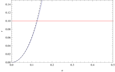
Figure 4: The scalar-to-tensor ratio as a function of $\alpha$ for $\gamma=2$, and for $N=60$ (black and dashed curve) and $N=40$ (blue curve). The upper red dashed line is the upper limit of the Planck allowed value for the scalar-to-tensor ratio $r=0.10$

Before closing, we need to stress the two important features of the present paper. Firstly, we showed that the slow-roll era may last for a shorter time, so for $N<50$, if some $e$-foldings occur during the constant-roll era. Secondly, in our approach, a graceful exit is possible, since it may occur during the slow-roll era, when $\epsilon,\eta\sim 1$. This was not possible in the constant-roll framework, since in most cases the constant-roll era is very stable.

IV Conclusions

In this work we studied smooth transitions from a constant-roll era to a slow-roll era. We examined the dynamics of the cosmological solution, and we investigated whether this solution is a stable and final attractor of the cosmological dynamical system. We performed both a numerical and analytical analysis, and as we showed, the cosmological solution $H(\varphi)$ is a stable attractor and also it is the final attractor of the system. So the cosmological system is led to a slow-roll era from a constant-roll era. Also, with regard to the slow-roll era, we investigated the resulting limiting form of the potential, which turned out to be a particular form of modular inflation. We made a thorough analysis of the free parameters space of the model, and we investigated that the model can be partially compatible with the Planck data, meaning that we did not achieve both the spectral index and the scalar-to-tensor ration to be compatible with the Planck data. However, this is very much model dependent. The new features that this work suggests are, firstly, the fact that the slow-roll era comes after the constant-roll, so in principle the inflationary era may end, since if the constant-roll era occurs last, it is very stable, so the possibility of exit is small. Secondly, and more importantly, the central idea of the paper is that a constant-roll and slow-roll era may occur together, and it is then possible that some $e$-foldings of the Universe occur during the constant-roll era, and in effect, the slow-roll era may last for $N<50-60$ $e$-foldings. Now the ultimate quest is to find a model which is completely viable and compatible with the Planck data. We need to note that we examined various cases which we did not include in the paper, and potentials that involve exponentials seem to occur if the slow-roll era occurs before the constant-roll era. We hope to address these issues in a future paper, and work is in progress towards this direction.

References

- (1) A. D. Linde, Lect. Notes Phys. 738 (2008) 1 [arXiv:0705.0164 [hep-th]].
- (2) D. S. Gorbunov and V. A. Rubakov, “Introduction to the theory of the early universe: Cosmological perturbations and inflationary theory,” Hackensack, USA: World Scientific (2011) 489 p;
- (3) A. Linde, arXiv:1402.0526 [hep-th];
- (4) D. H. Lyth and A. Riotto, Phys. Rept. 314 (1999) 1 [hep-ph/9807278].
- (5) K. Bamba and S. D. Odintsov, Symmetry 7 (2015) 1, 220 [arXiv:1503.00442 [hep-th]]
- (6) S. Nojiri and S. D. Odintsov, eConf C 0602061 (2006) 06 [Int. J. Geom. Meth. Mod. Phys. 4 (2007) 115] [hep-th/0601213].
- (7) S. Capozziello and M. De Laurentis, Phys. Rept. 509 (2011) 167 [arXiv:1108.6266 [gr-qc]].
- (8) V. Faraoni and S. Capozziello, Fundam. Theor. Phys. 170 (2010).
- (9) S. Nojiri and S. D. Odintsov, Phys. Rept. 505 (2011) 59 [arXiv:1011.0544 [gr-qc]].
- (10) T. Clifton, P. G. Ferreira, A. Padilla and C. Skordis, Phys. Rept. 513 (2012) 1 [arXiv:1106.2476 [astro-ph.CO]].
- (11) S. Nojiri, S. D. Odintsov and V. K. Oikonomou, arXiv:1705.11098 [gr-qc].
- (12) P. A. R. Ade et al. [Planck Collaboration], Astron. Astrophys. 594 (2016) A20 [arXiv:1502.02114 [astro-ph.CO]].
- (13) I. Ben-Dayan, R. Brustein and S. P. de Alwis, JCAP 0807 (2008) 011 doi:10.1088/1475-7516/2008/07/011 [arXiv:0802.3160 [hep-th]].
- (14) X. Chen, Adv. Astron. 2010 (2010) 638979 doi:10.1155/2010/638979 [arXiv:1002.1416 [astro-ph.CO]].
- (15) S. Inoue and J. Yokoyama, Phys. Lett. B 524 (2002) 15 doi:10.1016/S0370-2693(01)01369-7 [hep-ph/0104083].
- (16) N. C. Tsamis and R. P. Woodard, Phys. Rev. D 69 (2004) 084005 doi:10.1103/PhysRevD.69.084005 [astro-ph/0307463].
- (17) W. H. Kinney, Phys. Rev. D 72 (2005) 023515 doi:10.1103/PhysRevD.72.023515 [gr-qc/0503017].
- (18) M. H. Namjoo, H. Firouzjahi and M. Sasaki, Europhys. Lett. 101 (2013) 39001 doi:10.1209/0295-5075/101/39001 [arXiv:1210.3692 [astro-ph.CO]].
- (19) J. Martin, H. Motohashi and T. Suyama, Phys. Rev. D 87 (2013) no.2, 023514 doi:10.1103/PhysRevD.87.023514 [arXiv:1211.0083 [astro-ph.CO]].
- (20) H. Motohashi, A. A. Starobinsky and J. Yokoyama, JCAP 1509 (2015) no.09, 018 doi:10.1088/1475-7516/2015/09/018 [arXiv:1411.5021 [astro-ph.CO]].
- (21) Y. F. Cai, J. O. Gong, D. G. Wang and Z. Wang, JCAP 1610 (2016) no.10, 017 doi:10.1088/1475-7516/2016/10/017 [arXiv:1607.07872 [astro-ph.CO]].
- (22) S. Hirano, T. Kobayashi and S. Yokoyama, Phys. Rev. D 94 (2016) no.10, 103515 doi:10.1103/PhysRevD.94.103515 [arXiv:1604.00141 [astro-ph.CO]].
- (23) L. Anguelova, Nucl. Phys. B 911 (2016) 480 doi:10.1016/j.nuclphysb.2016.08.020 [arXiv:1512.08556 [hep-th]].
- (24) J. L. Cook and L. M. Krauss, JCAP 1603 (2016) no.03, 028 doi:10.1088/1475-7516/2016/03/028 [arXiv:1508.03647 [astro-ph.CO]].
- (25) K. S. Kumar, J. Marto, P. Vargas Moniz and S. Das, JCAP 1604 (2016) no.04, 005 doi:10.1088/1475-7516/2016/04/005 [arXiv:1506.05366 [gr-qc]].
- (26) S. D. Odintsov and V. K. Oikonomou, JCAP 1704 (2017) no.04, 041 doi:10.1088/1475-7516/2017/04/041 [arXiv:1703.02853 [gr-qc]].
- (27) S. D. Odintsov and V. K. Oikonomou, Phys. Rev. D 96 (2017) no.2, 024029 doi:10.1103/PhysRevD.96.024029 [arXiv:1704.02931 [gr-qc]].
- (28) S. Nojiri, S. D. Odintsov and V. K. Oikonomou, arXiv:1704.05945 [gr-qc].
- (29) Q. Fei, Y. Gong, J. Lin and Z. Yi, arXiv:1705.02545 [gr-qc].
- (30) Q. Gao, Sci. China Phys. Mech. Astron. 60 (2017) no.9, 090411 doi:10.1007/s11433-017-9065-4 [arXiv:1704.08559 [astro-ph.CO]].
- (31) Q. Gao and Y. Gong, “Reconstruction of extended inflationary potentials for attractors,” arXiv:1703.02220 [gr-qc].
- (32) J. Lin, Q. Gao and Y. Gong, Mon. Not. Roy. Astron. Soc. 459, no. 4, 4029 (2016) [arXiv:1508.07145 [gr-qc]].
- (33) A. R. Liddle, P. Parsons and J. D. Barrow, Phys. Rev. D 50 (1994) 7222 doi:10.1103/PhysRevD.50.7222 [astro-ph/9408015].