Time-Dependent Observables in Heavy Ion Collisions II: in Search of Pressure Isotropization in the $\varphi^{4}$ Theory

Abstract

To understand the dynamics of thermalization in heavy ion collisions in the perturbative framework it is essential to first find corrections to the free-streaming classical gluon fields of the McLerran–Venugopalan model. The corrections that lead to deviations from free streaming (and that dominate at late proper time) would provide evidence for the onset of isotropization (and, possibly, thermalization) of the produced medium. To find such corrections we calculate the late-time two-point Green function and the energy-momentum tensor due to a single $2\to 2$ scattering process involving two classical fields. To make the calculation tractable we employ the scalar $\varphi^{4}$ theory instead of QCD. We compare our exact diagrammatic results for these quantities to those in kinetic theory and find disagreement between the two. The disagreement is in the dependence on the proper time $\tau$ and, for the case of the two-point function, is also in the dependence on the space-time rapidity $\eta$: the exact diagrammatic calculation is, in fact, consistent with the free streaming scenario. Kinetic theory predicts a build-up of longitudinal pressure, which, however, is not observed in the exact calculation. We conclude that we find no evidence for the beginning of the transition from the free-streaming classical fields to the kinetic theory description of the produced matter after a single $2\to 2$ rescattering.

1 Introduction

The problem of isotropization and thermalization of the medium produced in ultra-relativistic heavy ion collisions is arguably the central theoretical problem in the field since it addresses the fundamental question of whether and how quark-gluon plasma (QGP) is formed in these collisions. Despite a number of theoretical efforts, the solution of this problem still remains elusive. Thermalization appears to be easier to tackle at strong (‘t Hooft) coupling in the framework of the anti-de Sitter/Conformal Field Theory (AdS/CFT) correspondence Maldacena:1997re ; Witten:1998qj : there it is possible to show that a collision of two shock waves results in the black hole formation in the AdS₅ bulk, corresponding to a thermal medium being formed at the boundary. This was demonstrated analytically (but indirectly) using the trapped surface analysis Gubser:2008pc ; Lin:2009pn ; Kovchegov:2009du and was directly observed in a numerical solution of Einstein equations Chesler:2009cy ; Chesler:2010bi . The weakness of the approach based on AdS/CFT correspondence is that the duality is for ${\cal N}=4$ super-Yang-Mills theory and not for quantum chromodynamics (QCD). Nevertheless, a consensus exists in the community that thermalization of the medium produced in high-energy collisions in strongly-coupled field theories is very likely to take place and to happen on a very short time scale.

The efforts to tackle the isotropization and thermalization problems at weak coupling have not achieved such a universal consensus. The initial break-through in the theoretical understanding of thermalization in QCD at weak coupling was the so-called ‘bottom-up thermalization’ proposal Baier:2000sb . In this scenario, the quark-gluon system that begins in an initial state due to saturated gluon fields created in nuclear collisions (dominated by the classical gluon fields of the McLerran-Venugopalan (MV) model McLerran:1993ni ; McLerran:1993ka ; McLerran:1994vd ; Krasnitz:1998ns ; Krasnitz:1999wc ; Krasnitz:2003nv ; Lappi:2003bi ) progresses to a thermalized isotropic medium due to $2\to 2$, $2\to 3$ and $3\to 2$ rescatterings. However, the qualitative arguments presented in Baier:2000sb have never been verified by explicit diagrammatic calculations. Moreover, in Arnold:2003rq ; Arnold:2004ih ; Arnold:2004ti it was pointed out that the bottom-up thermalization scenario may be invalidated by the occurrence of plasma instabilities, which could be present due to the momentum-space anisotropy of the initial non-equilibrium gluonic medium. Numerical simulations of these instabilities appear to demonstrate that the growth of instabilities is stopped due to the non-Abelian nature of strong interactions Rebhan:2004ur ; Romatschke:2006nk , possibly reinstating the original ‘bottom-up’ scenario. Alternative approaches Berges:2013fga apply classical Yang-Mills dynamics to confirm the parametric scaling of the observables predicted in the first stage of the ‘bottom-up’ thermalization Baier:2000sb , and possibly leading to eventual thermalization of the medium Gelis:2013rba : however, the resulting classical dynamics appears to be non-renormalizable Epelbaum:2014yja ; Epelbaum:2014mfa .

Yet another weakly-coupled approach to thermalization is based on Boltzmann equation. The applicability of Boltzmann equation to description of the medium produced in late stages of heavy ion collisions was argued in Mueller:2002gd ; Arnold:2002zm (with the Vlasov–Boltzmann equation used in the instability studies mentioned above). Boltzmann equation dynamics appears to lead to thermalization of the produced medium Kurkela:2015qoa , confirming the bottom-up thermalization scenario. However, the existing literature lacks a side-by-side comparison of Boltzmann equation with the explicit diagram calculation for heavy ion collisions: such a comparison is needed to either validate the applicability of the Boltzmann equation to heavy ion collisions or to prove otherwise. Performing such a cross-check is the main goal of the present work. In Mueller:2002gd a correspondence was established between the Boltzmann equation containing only the order-$f^{3}$ part of the collision term and the classical gluon fields at late times (and, hence, the late-time limit of the Feynman diagrams describing the collision in the classical approximation). However, the correspondence was never checked for the Boltzmann equation with the order-$f^{2}$ part of the collision term and the diagrams describing some correction to the classical fields of the MV model. This will be performed below.

In more general terms, many perturbative thermalization scenarios assume that the classical gluon fields of the MV model become sub-leading at late proper times in the collisions, being superseded by fields produced by some other dynamics, for instance due to the Boltzmann equation. However, no explicit calculation of Feynman diagrams exists in the literature which starts with the actual collision of two large nuclei, identifies a particular diagrammatic correction to the classical gluon fields and shows explicitly that such a correction becomes dominant at late times. The absence of such calculations is probably attributable to their complexity. However, an approach like this would have been natural in the saturation/Color Glass Condensate (CGC) framework Gribov:1984tu ; Iancu:2003xm ; Weigert:2005us ; Jalilian-Marian:2005jf ; Gelis:2010nm ; Albacete:2014fwa ; KovchegovLevin . There (and elsewhere in perturbative calculations in field theory) one usually starts with the tree-level leading-order contribution, which is often classical. The leading-order contribution receives corrections due to quantum fluctuations, leading parts of which may be resummed using evolution equations. This program has been carried out for the case of deep inelastic scattering (DIS) at small Bjorken $x$, where the leading order contribution to unpolarized DIS structure functions is given by the Glauber–Mueller quasi-classical multiple rescatterings Mueller:1989st , and the quantum corrections resumming logarithms of $1/x$ are included via the Balitsky–Kovchegov (BK) Balitsky:1995ub ; Balitsky:1998ya ; Kovchegov:1999yj ; Kovchegov:1999ua and Jalilian-Marian–Iancu–McLerran–Weigert–Leonidov–Kovner (JIMWLK) evolution equations Jalilian-Marian:1997dw ; Jalilian-Marian:1997gr ; Iancu:2001ad ; Iancu:2000hn .

For heavy ion collisions analyzed in the saturation framework the leading contribution to, say, the energy-momentum tensor of the produced medium is given by the classical gluon field of the MV model McLerran:1993ni ; McLerran:1993ka ; McLerran:1994vd ; Krasnitz:1998ns ; Krasnitz:1999wc ; Krasnitz:2003nv ; Lappi:2003bi . This is already a very difficult calculation, only possible to be fully done numerically due to the complexity of the analytic attempts Balitsky:2004rr ; Chirilli:2015tea (see Kovner:1995ts ; Kovner:1995ja ; Kovchegov:1997ke ; Kovchegov:1998bi ; Dumitru:2001ux for perturbative results valid for proton-proton and proton-nucleus collisions). The numerical calculations Krasnitz:1998ns ; Krasnitz:1999wc ; Krasnitz:2003nv ; Lappi:2003bi indicate that the classical gluon fields lead to a free-streaming medium, characterized by zero longitudinal pressure $P_{L}=0$ and the energy density $\epsilon=2\,P_{T}\sim 1/\tau$ at late proper times $\tau\gg 1/Q_{s}$. (Here $P_{T}$ and $P_{L}$ are the transverse and longitudinal pressures at mid-rapidity, $\tau=\sqrt{t^{2}-z^{2}}$ is the proper time, and $Q_{s}$ is the classical gluon saturation scale.) Quantum corrections to the classical energy-momentum tensor resumming leading logarithms of $1/x$ were addressed in Gelis:2008rw ; Gelis:2008ad , where it was argued that such corrections can be resummed using the JIMWLK evolution equation for the weight functionals of the color charge densities in the two nuclei. The resulting gluon fields are still obtained by solving the classical Yang-Mills equations, but now with the JIMWLK-modified distribution of color sources. Therefore, such small-$x$ evolution corrections still lead to a classical free-streaming energy-momentum tensor and are not related to isotropization or thermalization of the medium.

The question of whether perturbative quantum corrections to the classical gluon fields which usher in isotropization and thermalization exist still remains open. Over a decade ago, one of the authors of this work tried looking for such corrections in Kovchegov:2005ss (see also Kovchegov:2005kn ). Having failed to find them, he argued that such corrections do not exist as long as one can define a gluon production cross section: hence, the end state of any perturbative (weakly-coupled) dynamics in heavy ion collisions was argued to always be a free-streaming bunch of particles Kovchegov:2005ss ; Kovchegov:2005kn .

The arguments of Kovchegov:2005ss ; Kovchegov:2005kn notwithstanding, potential candidates for the isotropization-inducing quantum corrections are the $2\to 2$ rescatterings as resummed by Boltzmann equation in the framework of kinetic theory. In the previous part I of this paper duplex WuKovchegov we showed that if one starts with the Boltzmann distribution function $f^{(0)}$ for the classical gluon fields of the MV model, and inserts it into the order-$f^{2}$ part of the collision term of the Boltzmann equation, solving the latter for a corrected distribution $f^{(1)}$, one indeed does obtain isotropization corrections to the $P_{L}=0$, $\epsilon\sim 1/\tau$ free-streaming behavior of the classical gluon medium. The remaining question is whether Boltzmann equation correctly represents the Feynman diagrams it purports to sum. In WuKovchegov we review the derivation of Boltzmann equation that exists in the literature, concentrating on the same case of a single $2\to 2$ rescattering of two classical gluon fields. The conclusion reached in WuKovchegov is that the underlying Feynman diagrams including the $2\to 2$ rescattering lead either to results consistent with Boltzmann equation prediction of to free-streaming depending on how the late-time limit is taken. Namely, denote by $\tau_{0}$ the time of the $2\to 2$ rescattering (assumed to be instantaneous in the derivation, which is valid at late times only when the gradient expansion becomes possible) and by $\tau$ the time in the argument of $f$ (that is, the time when we measure the particle in question). For the Boltzmann equation to be valid, the particles (gluons) must approximately go on mass-shell both in the time after they are produced in a collision but before they rescatter and in the time after they rescatter but before they are detected. This means that time intervals $\tau_{0}$ and $\tau-\tau_{0}$ should be sufficiently long. While it is clear that for $\tau_{0}$ “sufficiently long” (on the average) means $\tau_{0}\gg 1/Q_{s}$, since $1/Q_{s}$ is the time it takes for the classical gluon fields to go on mass shell, it is less clear what “sufficiently long” means for $\tau-\tau_{0}$. In WuKovchegov we consider two options,

• $\tau-\tau_{0}\gg\frac{1}{Q_{s}}$,       $\tau_{0}\gg 1/Q_{s}$;

• $\tau-\tau_{0}\gg\tau_{0}\gg 1/Q_{s}$

and show that the ordering (i) yields results consistent with the Boltzmann equation, while the ordering (ii) leads to free streaming and is not consistent with the Boltzmann equation. Unfortunately the calculation performed in WuKovchegov (along with the earlier arguments in favor of Boltzmann equation) was too coarse to tell us whether the ordering (i) or the ordering (ii) follows from the full Feynman diagram calculation. It is the goal of the present paper to resolve this ambiguity, at least in the framework of the $\varphi^{4}$ theory that we use for simplicity instead of QCD.

Below we will calculate the Feynman diagrams contributing to the $2\to 2$ rescattering of two classical fields using the Schwinger-Keldysh formalism. As we have already mentioned, we will use the scalar $\varphi^{4}$ theory coupled to an external current Gelis:2006yv for simplicity. Without going into detail of the scalar particle production (though one could think of the Higgs production via gluon fusion), we assume that two scalar particles were produced in the collision with their distribution given by the two-point correlation functions very similar to that for the classical gluon fields in the saturation/CGC physics. (These two particles do not have to be on mass shell.) The setup of the problem is presented in Sec. 2 below. The particles rescatter via the $2\to 2$ process, which is simpler in the $\varphi^{4}$ theory than in QCD: for instance, this interaction is truly instantaneous in the $\varphi^{4}$ theory. The two-point coordinate-space correlation function $G(x_{1},x_{2})$ resulting from the rescattering is calculated in Sec. 3. A calculation of the mixed-representation Green function $G(X,P)$ (that is commonly used in derivations of Boltzmann equation) resulting from the same $2\to 2$ rescattering process is presented in Sec. 4. (Sec. 3 also contains a calculation of the corresponding energy-momentum tensor.) Both Green function calculations lead to the result consistent with free streaming and hence with the case (ii). Therefore, we see no evidence supporting the use of Boltzmann equation in describing the (perturbative) dynamics of the medium produced in heavy ion collisions. Our conclusions are summarized in Sec. 5.

2 Isotropization problem for the $\varphi^{4}$ theory

2.1 Classical two-point correlation function

The two-point $22$ correlation function due to the lowest-order classical gluon fields in the MV model was calculated in WuKovchegov using the $A^{+}=0$ light-cone gauge. The result is

$$G_{22}^{a\mu,b\nu}(k,k^{\prime})\equiv \langle A^{a\mu}(k)\,A^{b\nu}(k^{\prime})\rangle=(2\pi)^{2}\delta(\underline{k}+\underline{k}^{\prime})\frac{i}{k^{2}+i\epsilon k^{0}}\frac{i}{k^{\,\prime\,2}+i\epsilon k^{\,\prime\,0}}$$

$$\times\left(-\frac{16\pi^{2}\alpha_{s}^{3}\,\delta^{ab}}{N_{c}}\right)\left(\frac{A}{S_{\perp}}\right)^{2}\frac{1}{(\underline{k}^{2})^{2}}\,\ln\frac{\underline{k}^{2}}{\Lambda^{2}}\,\sum\limits_{\lambda=\pm}\epsilon_{\lambda}^{\mu}(k)\epsilon_{\lambda}^{*\nu}(-k^{\prime})$$ (1)

with the polarization vector

$$\epsilon^{\mu}_{\lambda}(k)=\left(0,\frac{\underline{\epsilon}_{\lambda}\cdot\underline{k}}{k^{+}},\underline{\epsilon}_{\lambda}\right)\qquad\text{and}\qquad\sum\limits_{\lambda=\pm}\epsilon_{\lambda}^{i}\epsilon^{*j}_{\lambda}=\delta^{ij}.$$ (2)

Here we assume the collision of two identical large nuclei with atomic numbers $A_{1}=A_{2}=A$, each of them shaped as a longitudinally-oriented cylinder with a very large cross-sectional area $S_{\perp}$. Underlined variables denote two-dimensional vectors in transverse plane, $\underline{v}=(v^{1},v^{2})$, while the light-cone variables are $v^{\pm}=(v^{0}\pm v^{3})/\sqrt{2}$ with $x^{3}=z$ the collision axis. The contributing diagrams for the correlator (2.1) are shown in Fig. 3 of WuKovchegov and are comprised of two sets of lowest-order gluon production diagrams (cf. Kovner:1995ts ; Kovner:1995ja ; Kovchegov:1997ke ).

As described above, it would be very interesting and important to find the perturbative correction to the correlator (2.1) due to a $2\to 2$ rescattering process involving two such Green functions. However, full calculation of the order-$\alpha_{s}^{2}$ correction to Eq. (2.1) involving two classical correlators (that is, a calculation of the order-$\alpha_{s}^{8}(A/S_{\perp})^{4}$ correlator) appears to be prohibitively complicated in QCD. Instead we will tackle a similar problem in massless $\varphi^{4}$ theory. To do so we first have to construct an analogue of the correlator (2.1) in the massless scalar theory. This is achieved by replacing the polarization sum in Eq. (2.1) by $(-1)$ and writing the rest of the expression as

$$G^{LO}_{22}(k,k^{\prime})\equiv\langle\varphi_{cl}(k)\,\varphi_{cl}(k^{\prime})\rangle=-\frac{i}{k^{2}+i\epsilon k^{0}}\,f(k_{T})\,(2\pi)^{2}\,\delta^{2}(\underline{k}+\underline{k}^{\prime})\,\frac{i}{k^{\,\prime\,2}+i\epsilon k^{\,\prime\,0}}$$ (3)

with $f(k_{T})$ a function of the magnitude of the transverse momentum $k_{T}=|\underline{k}|$ which falls off rather fast at large $k_{T}$ and is infrared (IR) finite due to saturation effects. The exact form of $f(k_{T})$ is not going to be important below. (This function is proportional to the $k_{T}$ spectrum $dN/d^{2}k_{T}dy$ of the produced particles in the classical approximation Kovchegov:2005ss .) The rapidity-independent correlation function (3) can not result from a collision of particles taken entirely in the scalar theory: instead, one can think of it as resulting from some gluon+gluon$\to$scalar fusion process, with the two gluons coming from the classical fields of the two colliding nuclei, as schematically shown in Fig. 1, where the shaded circle represents an effective gluon+gluon$\to$scalar vertex. Higgs production through gluon fusion (via a top-quark loop) is one example of such a process (though of course Higgs is massive, unlike the massless scalar considered here). Let us stress one more time that the exact origin of the correlation function (3) is not important here: what is important is that it carries the main features of the gluon correlation function (2.1).

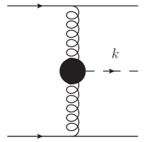
Figure 1: Scalar particle production as envisioned here, with the solid lines denoting colliding quarks in the two nuclei and the dashed line denoting the scalar particle. The shaded circle may represent a quark loop, as would be the case in the Higgs production.

Our notation for the correlation function (3) is shown in Fig. 2, where the Feynman diagrams contributing to the correlator are summarily shown by a green oval.

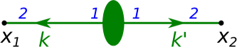
Figure 2: The classical correlation function from Eq. (3) or Eq. (5) with the green oval denoting all the possible contributing Feynman diagrams (like the ‘square’ of the one shown in Fig. 1). Solid lines from now on represent the scalar field. The indices $1$ and $2$ denote the type of the propagator in the Schwinger–Keldysh formalism.

In coordinate space the Green function (3) is given by the Fourier transform

$$G^{LO}_{22}(x_{1},x_{2})=\int\frac{d^{4}k}{(2\pi)^{4}}\,\frac{d^{4}k^{\prime}}{(2\pi)^{4}}\,e^{-ik\cdot x_{1}-ik^{\prime}\cdot x_{2}}\,G^{LO}_{22}(k,k^{\prime}).$$ (4)

Employing the integrals in the appendices of Kovchegov:2005ss we obtain

$$G^{LO}_{22}(x_{1},x_{2})=\frac{1}{4}\int\frac{d^{2}k_{T}}{(2\pi)^{2}}\,e^{i\underline{k}\cdot\underline{x}_{12}}\,f(k_{T})\,J_{0}(k_{T}\,\tau_{1})\,J_{0}(k_{T}\,\tau_{2}),$$ (5)

where $\underline{x}_{12}=\underline{x}_{1}-\underline{x}_{2}$ and $\tau_{1}=\sqrt{2x_{1}^{+}x_{1}^{-}}$, $\tau_{2}=\sqrt{2x_{2}^{+}x_{2}^{-}}$. Using the large-argument asymptotics of Bessel functions we conclude that

$$G^{LO}_{22}(x_{1},x_{2})\Bigg{|}_{\tau_{1}=\tau_{2}=\tau\gg\frac{1}{Q_{s}}}=\frac{1}{4\pi\tau}\int\frac{d^{2}k_{T}}{(2\pi)^{2}}\,e^{i\underline{k}\cdot\underline{x}_{12}}\,\frac{f(k_{T})}{k_{T}},$$ (6)

where we have averaged the cosine squared over time. (We have also employed the fact that $f(k_{T})$ is regulated by the saturation scale $Q_{s}$ in the IR, such that the $k_{T}\approx 0$ region does not contribute significantly to the integral.)

Importantly the classical correlation function scales as

$$G^{LO}_{22}(x_{1},x_{2})\Bigg{|}_{\tau_{1}=\tau_{2}=\tau\gg\frac{1}{Q_{s}}}\propto\frac{1}{\tau},$$ (7)

which is a tell-tale sign of free streaming. To understand this better, let us calculate the energy-momentum tensor corresponding to this classical dynamics. The correlation function (5) is independent of the space-time rapidities $\eta_{1}=(1/2)\ln(x_{1}^{+}/x_{1}^{-})$ and $\eta_{2}=(1/2)\ln(x_{2}^{+}/x_{2}^{-})$. It is natural to conclude, and we will see shortly that this is indeed the case, that the corresponding energy-momentum tensor is also rapidity-independent.

The most general energy-momentum tensor for a medium produced in a high-energy collision of two large nuclei with the rapidity-independent matter distribution can be parametrized in terms of the energy density $\epsilon$ and transverse and longitudinal pressures $P_{T},P_{L}$ as

$$T^{++}\,=\,[\epsilon(\tau)+P_{L}(\tau)]\,\left(\frac{x^{+}}{\tau}\right)^{2},~{}$$

$$T^{--}\,=\,[\epsilon(\tau)+P_{L}(\tau)]\,\left(\frac{x^{-}}{\tau}\right)^{2},~{}$$

$$T^{+-}\,=\,[\epsilon(\tau)-P_{L}(\tau)]\,\frac{1}{2},~{}$$

$$T^{ij}\,=\,\delta^{ij}\,P_{T}(\tau).$$ (8)

(We employ translational invariance in the transverse plane due to the nuclei being very large.) At mid-rapidity ($z=0$) the tensor (2.1) looks like

$$T^{\mu\nu}(z=0)=\left(\begin{matrix}\epsilon(\tau)&0&0&0\\ 0&P_{T}(\tau)&0&0\\ 0&0&P_{T}(\tau)&0\\ 0&0&0&P_{L}(\tau)\\ \end{matrix}\right)$$ (9)

in the $t,x,y,z$ coordinates. It is also useful to note that the energy-momentum conservation

$$\partial_{\mu}T^{\mu\nu}\,=\,0$$ (10)

yields

$$\frac{d\epsilon}{d\tau}\,=\,-\frac{\epsilon+P_{L}}{\tau}.$$ (11)

The energy-momentum tensor in the massless $\varphi^{4}$ theory with the Lagrangian density

$${\cal L}=\frac{1}{2}\partial_{\mu}\varphi\,\partial^{\mu}\varphi-\frac{\lambda}{4!}\,\varphi^{4}$$ (12)

is given by

$$T^{\mu\nu}=\langle\partial^{\mu}\varphi\,\partial^{\nu}\varphi-g^{\mu\nu}\,{\cal L}\rangle=\left\langle\partial^{\mu}\varphi\,\partial^{\nu}\varphi-g^{\mu\nu}\,\left[\frac{1}{2}\partial_{\alpha}\varphi\,\partial^{\alpha}\varphi-\frac{\lambda}{4!}\,\varphi^{4}\right]\right\rangle.$$ (13)

With the two-point correlation function decaying at late times as shown in Eq. (7), it is natural to conclude that the four-point correlation function decays twice as fast and is, therefore, negligible in Eq. (13) taken at late times. We therefore arrive at

$$T^{\mu\nu}_{LO}\Bigg{|}_{\tau\gg\frac{1}{Q_{s}}}=\left[\partial_{1}^{\mu}\,\partial_{2}^{\nu}-\frac{1}{2}g^{\mu\nu}\,\partial_{1\,\alpha}\,\partial_{2}^{\alpha}\right]\,G^{LO}_{22}(x_{1},x_{2})\Bigg{|}_{x_{1}=x_{2},\ \tau\gg\frac{1}{Q_{s}}}\,.$$ (14)

Here the subscripts $1$ and $2$ denote derivatives with respect to $x_{1}$ and $x_{2}$ respectively. Substituting the Green function from Eq. (5) we find (cf. Kovchegov:2005ss ; Lappi:2006hq , the $J_{0}\leftrightarrow J_{1}$ difference in $p_{T}$ is inconsequential at late times)

$$\epsilon=\frac{1}{8}\,\int\frac{d^{2}k_{T}}{(2\pi)^{2}}\,f(k_{T})\,k_{T}^{2}\,\left\{\left[J_{0}(k_{T}\,\tau)\right]^{2}+\left[J_{1}(k_{T}\,\tau)\right]^{2}\right\},$$ (15a)

$$P_{T}=\frac{1}{8}\,\int\frac{d^{2}k_{T}}{(2\pi)^{2}}\,f(k_{T})\,k_{T}^{2}\,\left[J_{1}(k_{T}\,\tau)\right]^{2}$$ (15b)

$$P_{L}=\frac{1}{8}\,\int\frac{d^{2}k_{T}}{(2\pi)^{2}}\,f(k_{T})\,k_{T}^{2}\,\left\{\left[J_{1}(k_{T}\,\tau)\right]^{2}-\left[J_{0}(k_{T}\,\tau)\right]^{2}\right\}$$ (15c)

for the classical medium at $\tau Q_{s}\gg 1$. Applying the late-time asymptotics to Eqs. (15) we arrive at

$$\epsilon=2\,P_{T}\sim\frac{1}{\tau},\ \ \ p_{L}=0.$$ (16)

This is a free-streaming anisotropic medium, with zero longitudinal pressure and a non-zero transverse pressure. In the full MV model, the classical gluon fields produced in a nuclear collision also lead to the free-streaming asymptotics of Eq. (16).

Note also that due to Eq. (11) the $\epsilon\sim 1/\tau$ scaling corresponds to $P_{L}=0$ and, hence, to free streaming. A more isotropic medium with non-zero $P_{L}>0$ would have the energy density $\epsilon$ falling off faster than $1/\tau$. The isotropization problem in heavy ion collisions can be formulated as follows: can one find (presumably quantum) corrections to the classical field correlator (3) modifying the free-streaming result (16) at late times in such a way as to generate a non-zero $p_{L}>0$, or, equivalently, give us the net energy density $\epsilon$ that decreases faster than $1/\tau$?

2.2 Boltzmann equation prediction for the two-point function after a single rescattering

Kinetic theory appears to give a positive answer to the above isotropization question. In WuKovchegov we show that using the classical particle distribution $f_{cl}=f^{(0)}$ resulting from the correlator (2.1), inserting it in the collision term of the Boltzmann equation, and solving the resulting equation for the new distribution $f^{(1)}$ gives the following components of the energy-momentum tensor:

$$\epsilon=\epsilon^{(0)}+\epsilon^{(1)}=\frac{A^{(0)}+\alpha_{s}^{2}\,A^{(1)}}{\tau}-\frac{\alpha_{s}^{2}\,B^{(1)}}{\tau}\,\ln\frac{\tau}{\tau_{0}},$$ (17a)

$$P_{T}=P_{T}^{(0)}+P_{T}^{(1)}=\frac{A^{(0)}+\alpha_{s}^{2}\,A^{(1)}-\alpha_{s}^{2}\,B^{(1)}}{\tau}-\frac{\alpha_{s}^{2}\,B^{(1)}}{\tau}\,\ln\frac{\tau}{\tau_{0}},$$ (17b)

$$P_{L}=P_{L}^{(1)}=\frac{\alpha_{s}^{2}\,B^{(1)}}{\tau}.$$ (17c)

Putting the strong coupling to zero in Eqs. (17), $\alpha_{s}=0$, we recover the leading-order classical free-streaming result (16) (with some coefficient $A^{(0)}$). The corrections due to the single iteration of the Boltzmann collision term enter at the order $\alpha_{s}^{2}$ in Eqs. (17) with some coefficients $A^{(1)}$ and $B^{(1)}$. (Note that $\tau_{0}$ is the lower cutoff for the applicability times of kinetic theory: it is applicable for $\tau>\tau_{0}$.) Since the pressure components in kinetic theory must be positive, we see that $B^{(1)}>0$. Therefore, the $B^{(1)}$-corrections in (17) appear to lead to $P_{L}>0$ and simultaneously make the energy density $\epsilon$ decrease faster than $1/\tau$. We see that kinetic theory predicts that a single $2\to 2$ rescattering of two classical fields would generate the first isotropization correction we are after. The remaining question is whether such correction arises in the full field-theoretical calculation.

The perturbative solution of Boltzmann equation from WuKovchegov is quite general and is valid for the $2\to 2$ collision term calculated in any theory. While the discussion in WuKovchegov concentrated on QCD with the expansion in Eqs. (17) being in powers of $\alpha_{s}$, it can be easily modified to apply to the scalar $\varphi^{4}$ theory in question here by simply replacing $\alpha_{s}\to\lambda$ everywhere. (All the appropriate constants and scattering amplitudes would be modified as well, but this would not matter so much for us since we are interested mainly in the form of the $\tau$-dependence of the energy-momentum tensor.) Equations (17) can be rewritten as

$$\epsilon=\epsilon^{(0)}+\epsilon^{(1)}=\frac{A^{(0)}+\lambda^{2}\,A^{(1)}}{\tau}-\frac{\lambda^{2}\,B^{(1)}}{\tau}\,\ln\frac{\tau}{\tau_{0}},$$ (18a)

$$P_{T}=P_{T}^{(0)}+P_{T}^{(1)}=\frac{A^{(0)}+\lambda^{2}\,A^{(1)}-\lambda^{2}\,B^{(1)}}{\tau}-\frac{\lambda^{2}\,B^{(1)}}{\tau}\,\ln\frac{\tau}{\tau_{0}},$$ (18b)

$$P_{L}=P_{L}^{(1)}=\frac{\lambda^{2}\,B^{(1)}}{\tau}.$$ (18c)

(It is understood that $A^{(0)}$, $A^{(1)}$, $B^{(1)}$ and possibly even $\tau_{0}$ are different in Eqs. (17) and (18).) Once again we observe that the kinetic theory has a specific prediction for the outcome of the single $2\to 2$ rescattering of two classical fields. In the remainder of this paper we will verify the results (18) by an explicit diagrammatic calculation.

3 Two-point correlation function with a single rescattering: Full diagrammatic calculation in momentum space

In this Section our aim is to calculate the late-times $\tau_{1},\tau_{2}$ asymptotics of the correlation function $G_{22}(x_{1},x_{2})$ due to a single $2\to 2$ rescattering involving two classical fields. The diagrams we want to calculate are shown in Fig. 3. The diagrams are labeled I, II, II’, III, and III’ with II’ and III’ obtainable from II and III by replacing $x_{1}\leftrightarrow x_{2}$ in them. In the kinetic theory language, diagrams I, II, and II’ correspond to the gain term in the (collision term of the) Boltzmann equation, while diagrams III and III’ correspond to the loss term. Below we will first calculate diagrams I, II, and II’ together, and then calculate diagrams III and III’.

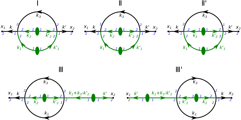
Figure 3: The diagrams for the $2\to 2$ rescattering correction to the classical field Green function that we calculate in this section. The green oval, along with the attached propagators, denote the classical correlation function.

3.1 Diagrams I, II, and II’

Let us start with diagram I. In momentum space one has

$$\text{Diag}_{\text{I}}(k,k^{\prime})= -\frac{\lambda^{2}}{2}\frac{i}{k^{2}+i\epsilon k^{0}}\,\frac{i}{k^{\,\prime\,2}+i\epsilon k^{\,\prime\,0}}$$

$$\times\frac{d^{4}k_{1}}{(2\pi)^{4}}\,\frac{d^{4}k^{\prime}_{1}}{(2\pi)^{4}}\,\frac{d^{4}k_{2}}{(2\pi)^{4}}\,\frac{d^{4}k^{\prime}_{2}}{(2\pi)^{4}}\,\frac{d^{4}k_{3}}{(2\pi)^{4}}\,(2\pi)^{4}\,\delta^{4}(k-k_{1}-k_{2}-k_{3})$$

$$\times(2\pi)^{4}\,\delta^{4}(k^{\prime}-k^{\prime}_{1}-k^{\prime}_{2}+k_{3})\,G^{LO}_{22}(k_{1},k^{\prime}_{1})\,G^{LO}_{22}(k_{2},k^{\prime}_{2})\,\pi\,\delta(k_{3}^{2})$$ (19)

with the leading-order classical correlation function given by (3). Substituting (3) into (3.1) and integrating out all the delta-functions (except for one) yields

$$\mbox{Diag}_{\text{I}}(k,k^{\prime})= -\frac{\lambda^{2}}{2}(2\pi)^{2}\delta^{2}(\underline{k}+\underline{k}^{\prime})G_{R}(k)G_{R}(k^{\prime})$$

$$\times\int\frac{d^{2}k_{1}}{(2\pi)^{2}}\,f(k_{1T})\,f(k_{2T})\,\int\frac{d^{4}k_{3}}{(2\pi)^{4}}\,\pi\,\delta(k_{3}^{2})$$

$$\times I_{1}(k^{+}-k_{3}^{+},k^{-}-k_{3}^{-},k_{1T},k_{2T})\,I_{1}(k^{\prime+}+k_{3}^{+},k^{\prime-}+k_{3}^{-},k_{1T},k_{2T})$$ (20)

with $\underline{k}_{2}=\underline{k}-\underline{k}_{1}-\underline{k}_{3}$ and the retarded scalar Green function

$$G_{R}(p)=\frac{i}{2(p^{+}+i\epsilon)(p^{-}+i\epsilon)-\underline{p}^{2}}.$$ (21)

In coordinate space one has

$$\mbox{Diagram I}= \,\int\frac{d^{4}k}{(2\pi)^{4}}\,\frac{d^{4}k^{\prime}}{(2\pi)^{4}}\,e^{-ik\cdot x_{1}-ik^{\prime}\cdot x_{2}}\,\text{Diag}_{\text{I}}(k,k^{\prime})$$

$$= -\frac{\lambda^{2}}{2}\,\int\limits_{-\infty}^{\infty}\frac{dk^{+}\,dk^{-}}{(2\pi)^{2}}\,e^{-ik^{+}x_{1}^{-}-ik^{-}x_{1}^{+}}\,\frac{i}{k^{2}+i\epsilon k^{0}}\,\int\limits_{-\infty}^{\infty}\frac{dk^{\prime+}dk^{\prime-}}{(2\pi)^{2}}\,e^{-ik^{\prime+}x^{-}_{2}-ik^{\prime-}x_{2}^{+}}$$

$$\times\frac{i}{k^{\,\prime\,2}+i\epsilon k^{\,\prime\,0}}\,\frac{d^{2}k}{(2\pi)^{2}}\frac{d^{2}k_{1}}{(2\pi)^{2}}\,f(k_{1T})\,f(k_{2T})\,e^{i\underline{k}\cdot\underline{x}_{12}}\,\frac{d^{4}k_{3}}{(2\pi)^{4}}\,\pi\,\delta(k_{3}^{2})$$

$$\times I_{1}(k^{+}-k_{3}^{+},k^{-}-k_{3}^{-},k_{1T},k_{2T})\,I_{1}(k^{\prime+}+k_{3}^{+},k^{\prime-}+k_{3}^{-},k_{1T},k_{2T}).$$ (22)

From now on it is implicitly understood that

$$\underline{k}^{\prime}=-\underline{k},\ \ \ \underline{k}_{2}=\underline{k}-\underline{k}_{1}-\underline{k}_{3}.$$ (23)

In arriving at Eq. (3.1) we have defined

$$I_{1}(q^{+},q^{-},p_{T},|\underline{q}-\underline{p}|)=\int\limits_{-\infty}^{\infty}\frac{dp^{+}dp^{-}}{(2\pi)^{2}}\,G_{R}(p)\,G_{R}(q-p).$$ (24)

Equation (3.1) can be written more compactly by defining

$$I_{3}(x^{+},x^{-},k_{T},k_{1T},k_{2T})=\int\limits_{-\infty}^{\infty}\frac{dk^{+}dk^{-}}{(2\pi)^{2}}\ e^{-ik^{+}x^{-}-ik^{-}x^{+}}\,G_{R}(k)$$

$$\times I_{1}(k^{+}-k_{3}^{+},k^{-}-k_{3}^{-},k_{1T},k_{2T}).$$ (25)

We obtain

$$\mbox{Diagram I}= -\frac{\lambda^{2}}{2}\,\int\frac{d^{2}k}{(2\pi)^{2}}\frac{d^{2}k_{1}}{(2\pi)^{2}}\,f(k_{1T})\,f(k_{2T})\,e^{i\underline{k}\cdot\underline{x}_{12}}\,\frac{d^{4}k_{3}}{(2\pi)^{4}}\,\pi\,\delta(k_{3}^{2})$$

$$\times I_{3}(x_{1}^{+},x_{1}^{-},k_{T},k_{1T},k_{2T})\,I_{3}(x_{2}^{+},x_{2}^{-},k_{T},k_{1T},k_{2T}).$$ (26)

While the exact evaluation of $I_{3}$ appears to be rather involved, we can obtain its late-time asymptotics. To do this we start with the full expression for $I_{3}$,

$$I_{3}(x^{+},x^{-},k_{T},k_{1T},k_{2T})= \int\limits_{-\infty}^{\infty}\frac{dk^{+}dk^{-}}{(2\pi)^{2}}\ e^{-ik^{+}x^{-}-ik^{-}x^{+}}\,G_{R}(k)$$

$$\times\int\limits_{-\infty}^{\infty}\frac{dk_{1}^{+}dk_{1}^{-}}{(2\pi)^{2}}\,G_{R}(k_{1})\,G_{R}(k-k_{3}-k_{1}),$$ (27)

and integrate over $k^{-}$ to obtain

$$I_{3}(x^{+},x^{-},k_{T},k_{1T},k_{2T})=\int\limits_{-\infty}^{\infty}\frac{dk^{+}}{2\pi}\,\frac{e^{-ik^{+}x^{-}-i\,\frac{k_{T}^{2}}{2(k^{+}+i\epsilon)}x^{+}}}{2(k^{+}+i\epsilon)}\,\int\limits_{-\infty}^{\infty}\frac{dk_{1}^{+}dk_{1}^{-}}{(2\pi)^{2}}\,G_{R}(k_{1})$$ (28)

$$\times\frac{-i}{2(k^{+}-k_{3}^{+}-k_{1}^{+}+i\epsilon)}\,\frac{1-e^{-i\left(k_{3}^{-}+k_{1}^{-}+\frac{k_{2T}^{2}}{2(k^{+}-k_{3}^{+}-k_{1}^{+}+i\epsilon)}-\frac{k_{T}^{2}}{2(k^{+}+i\epsilon)}\right)\,x^{+}}}{k_{3}^{-}+k_{1}^{-}+\frac{k_{2T}^{2}}{2(k^{+}-k_{3}^{+}-k_{1}^{+}+i\epsilon)}-\frac{k_{T}^{2}}{2(k^{+}+i\epsilon)}},$$

in a form reminiscent of the light-cone perturbation theory (LCPT) Lepage:1980fj .

Now let us apply the large-$\tau$ limit to Eq. (28). Note that since the limit of a product is equal to the product of the limits, we can first take the large-$x^{+}$ limit of the last fraction in Eq. (28). To do so we observe that

$$\lim_{x\to+\infty}\frac{1-e^{-i\,a\,x}}{a}=\frac{1}{a-i\,\epsilon}$$ (29)

in the distribution sense. Indeed this is true for any function $h(a)$ of real variable $a$ decomposable into a Fourier integral,

$$h(a)=\int\limits_{-\infty}^{\infty}d\xi\,e^{i\,a\,\xi}\,{\tilde{h}}(\xi).$$ (30)

To see this we simply point out that

$$\lim_{x\to+\infty}\int\limits_{-\infty}^{\infty}da\,e^{i\,a\,\xi}\,\frac{1-e^{-i\,a\,x}}{a} =\lim_{x\to+\infty}\int\limits_{-\infty}^{\infty}da\,e^{i\,a\,\xi}\,\frac{1-e^{-i\,a\,x}}{a-i\epsilon}$$

$$=2\pi i\,\lim_{x\to+\infty}[\theta(\xi)-\theta(\xi-x)]=2\pi i\,\theta(\xi),$$ (31)

which is identical to the same convolution of $e^{i\,a\,\xi}$ with the right-hand side of Eq. (29),

$$\int\limits_{-\infty}^{\infty}da\,e^{i\,a\,\xi}\,\frac{1}{a-i\,\epsilon}=2\pi i\,\theta(\xi).$$ (32)

Applying Eq. (29) to the last fraction in Eq. (28) after neglecting all the $i\epsilon$’s in the exponent we obtain

$$I_{3}(x^{+},x^{-},k_{T}, \,k_{1T},k_{2T})\bigg{|}_{\tau\to\infty}=\int\limits_{-\infty}^{\infty}\frac{dk^{+}}{2\pi}\,\frac{e^{-ik^{+}x^{-}-i\,\frac{k_{T}^{2}}{2(k^{+}+i\epsilon)}x^{+}}}{2(k^{+}+i\epsilon)}\,\int\limits_{-\infty}^{\infty}\frac{dk_{1}^{+}dk_{1}^{-}}{(2\pi)^{2}}\,G_{R}(k_{1})$$

$$\times\frac{-i}{2(k^{+}-k_{3}^{+}-k_{1}^{+}+i\epsilon)}\,\frac{1}{k_{3}^{-}+k_{1}^{-}+\frac{k_{2T}^{2}}{2(k^{+}-k_{3}^{+}-k_{1}^{+}+i\epsilon)}-k^{-}-i\epsilon},$$ (33)

where by $k^{-}$ we now imply its on-shell value,

$$k^{-}=\frac{k_{T}^{2}}{2k^{+}}.$$ (34)

Equation (3.1) easily simplifies into

$$I_{3}(x^{+},x^{-},k_{T},k_{1T},k_{2T})\bigg{|}_{\tau\to\infty}=\int\limits_{-\infty}^{\infty}\frac{dk^{+}}{2\pi} \,\frac{e^{-ik^{+}x^{-}-i\,\frac{k_{T}^{2}}{2(k^{+}+i\epsilon)}x^{+}}}{2(k^{+}+i\epsilon)}$$

$$\times\,\int\limits_{-\infty}^{\infty}\frac{dk_{1}^{+}dk_{1}^{-}}{(2\pi)^{2}}\,G_{R}(k_{1})\,G_{R}(k-k_{3}-k_{1}),$$ (35)

which, with the help of Eq. (24) becomes

$$I_{3}(x^{+},x^{-},k_{T},k_{1T},k_{2T})\bigg{|}_{\tau\to\infty}=\int\limits_{-\infty}^{\infty}\frac{dk^{+}}{2\pi}\,\frac{e^{-ik^{+}x^{-}-i\,\frac{k_{T}^{2}}{2(k^{+}+i\epsilon)}x^{+}}}{2(k^{+}+i\epsilon)}\,I_{1}(k^{+}-k_{3}^{+},k^{-}-k_{3}^{-},k_{1T},k_{2T}).$$ (36)

Here again $k^{-}$ is given by Eq. (34).

Substituting Eq. (36) into Eq. (3.1) yields

Diagram I $$\,\bigg{|}_{\tau_{1},\tau_{2}\to\infty}=-\frac{\lambda^{2}}{2}\,\int\limits_{-\infty}^{\infty}\frac{dk^{+}}{2\pi}\,\frac{e^{-ik^{+}x_{1}^{-}-i\,\frac{k_{T}^{2}}{2(k^{+}+i\epsilon)}x_{1}^{+}}}{2(k^{+}+i\epsilon)}\,\int\limits_{-\infty}^{\infty}\frac{dk^{\prime+}}{2\pi}\,\frac{e^{-ik^{\prime+}x_{2}^{-}-i\,\frac{k_{T}^{2}}{2(k^{\prime+}+i\epsilon)}x_{2}^{+}}}{2(k^{\prime+}+i\epsilon)}$$

$$\times\,\frac{d^{2}k}{(2\pi)^{2}}\frac{d^{2}k_{1}}{(2\pi)^{2}}\,f(k_{1T})\,f(k_{2T})\,e^{i\underline{k}\cdot\underline{x}_{12}}\,\frac{d^{4}k_{3}}{(2\pi)^{4}}\,\pi\,\delta(k_{3}^{2})$$

$$\times\,I_{1}(k^{+}-k_{3}^{+},k^{-}-k_{3}^{-},k_{1T},k_{2T})\,I_{1}(k^{\prime+}+k_{3}^{+},k^{\prime-}+k_{3}^{-},k_{1T},k_{2T}).$$ (37)

Note that here and throughout the paper, when writing $\tau\to\infty$, we mean large but finite proper time $\tau$, that is $\tau\,p_{T}\gg 1$ with $p_{T}$ being any of the transverse momenta in the problem.

For now we leave the diagram I as evaluated in Eq. (3.1) and turn our attention to diagrams II and II’. Employing Eq. (3) and integrating over all delta-functions except for one in diagrams II and II’ gives in momentum space

$$\mbox{Diag}_{\mbox{II}}(k,k^{\prime})=-\frac{\lambda^{2}}{2}(2\pi)^{2}\delta^{2}(\underline{k}+\underline{k}^{\prime})\int\frac{d^{2}k_{1}}{(2\pi)^{2}}\,f(k_{1T})\,f(k_{2T})$$

$$\times\int\,\frac{d^{4}k_{3}}{(2\pi)^{4}}\,\pi\left[\delta(k^{2})G_{A}(k_{3})G_{R}(k^{\prime})+G_{R}(k)G_{R}(k_{3})\delta(k^{\prime 2})\right]\,$$

$$\times\,I_{1}(k^{+}-k_{3}^{+},k^{-}-k_{3}^{-},k_{1T},k_{2T})\,I_{1}(k^{\prime+}+k_{3}^{+},k^{\prime-}+k_{3}^{-},k_{1T},k_{2T}).$$ (38)

In coordinate space we have

$$\mbox{Diagrams II+II'}=\,\int\frac{d^{4}k}{(2\pi)^{4}}\,\frac{d^{4}k^{\prime}}{(2\pi)^{4}}\,e^{-ik\cdot x_{1}-ik^{\prime}\cdot x_{2}}\mbox{Diag}_{\mbox{II}}(k,k^{\prime})$$ (39)

$$=-\frac{\lambda^{2}}{2}\,\int\limits_{-\infty}^{\infty}\frac{dk^{+}}{8\pi|k^{+}|}\,e^{-ik^{+}x_{1}^{-}-i\,\frac{k_{T}^{2}}{2k^{+}}x_{1}^{+}}\frac{d^{2}k}{(2\pi)^{2}}\frac{d^{2}k_{1}}{(2\pi)^{2}}\,f(k_{1T})\,f(k_{2T})\,e^{i\underline{k}\cdot\underline{x}_{12}}$$

$$\times\,\frac{d^{4}k_{3}}{(2\pi)^{4}}\,\frac{i}{k_{3}^{2}-i\epsilon k_{3}^{0}}\,I_{3}(x_{2}^{+},x_{2}^{-},k_{T},k_{1T},k_{2T})\,I_{1}(k^{+}-k_{3}^{+},k^{-}-k_{3}^{-},k_{1T},k_{2T})+(x_{1}\leftrightarrow x_{2})$$

with $k^{-}$ given by Eq. (34). To study the late-time asymptotics of diagrams II and II’ we employ Eq. (36). This gives

$$\mbox{Diagrams II+II'}=-\frac{\lambda^{2}}{2}\,\int\limits_{-\infty}^{\infty}\frac{dk^{+}}{8\pi|k^{+}|}\,e^{-ik^{+}x_{1}^{-}-i\,\frac{k_{T}^{2}}{2k^{+}}x_{1}^{+}}\int\limits_{-\infty}^{\infty}\frac{dk^{\prime+}}{2\pi}\,\frac{e^{-ik^{\prime+}x_{2}^{-}-i\,\frac{k_{T}^{2}}{2(k^{\prime+}+i\epsilon)}x_{2}^{+}}}{2(k^{\prime+}+i\epsilon)}$$

$$\times\,\frac{d^{2}k}{(2\pi)^{2}}\frac{d^{2}k_{1}}{(2\pi)^{2}}\,f(k_{1T})\,f(k_{2T})\,e^{i\underline{k}\cdot\underline{x}_{12}}\,\frac{d^{4}k_{3}}{(2\pi)^{4}}\,\frac{i}{k_{3}^{2}-i\epsilon k_{3}^{0}}$$

$$\times\,I_{1}(k^{+}-k_{3}^{+},k^{-}-k_{3}^{-},k_{1T},k_{2T})\,I_{1}(k^{\prime+}+k_{3}^{+},k^{\prime-}+k_{3}^{-},k_{1T},k_{2T})+(x_{1}\leftrightarrow x_{2}).$$ (40)

Adding diagrams I, II, and II’ given by Eqs. (3.1) and Eq. (3.1) together we arrive at

$$\mbox{I+II+II'}\,\bigg{|}_{\tau_{1},\tau_{2}\to\infty}=-\frac{\lambda^{2}}{2}\,\int\limits_{-\infty}^{\infty}\frac{dk^{+}}{2\pi}\,\frac{e^{-ik^{+}x_{1}^{-}-i\,\frac{k_{T}^{2}}{2(k^{+}+i\epsilon)}x_{1}^{+}}}{2(k^{+}+i\epsilon)}\,\int\limits_{-\infty}^{\infty}\frac{dk^{\prime+}}{2\pi}\,\frac{e^{-ik^{\prime+}x_{2}^{-}-i\,\frac{k_{T}^{2}}{2(k^{\prime+}+i\epsilon)}x_{2}^{+}}}{2(k^{\prime+}+i\epsilon)}$$

$$\times\,\frac{d^{2}k}{(2\pi)^{2}}\frac{d^{2}k_{1}}{(2\pi)^{2}}\,f(k_{1T})\,f(k_{2T})\,e^{i\underline{k}\cdot\underline{x}_{12}}\,\frac{d^{4}k_{3}}{(2\pi)^{4}}$$

$$\times\,\frac{1}{2}\,\left[2\pi\,\delta(k_{3}^{2})+\mbox{Sign}(k^{+})\frac{i}{k_{3}^{2}-i\epsilon k_{3}^{0}}+\mbox{Sign}(k^{\prime+})\frac{i}{k_{3}^{2}+i\epsilon k_{3}^{0}}\right]$$

$$\times\,I_{1}(k^{+}-k_{3}^{+},k^{-}-k_{3}^{-},k_{1T},k_{2T})\,I_{1}(k^{\prime+}+k_{3}^{+},k^{\prime-}+k_{3}^{-},k_{1T},k_{2T}).$$ (41)

The late-time asymptotics of diagrams I, II and II’ given by Eq. (3.1) is dominated by the saddle points of the $k^{+}$ and $k^{\prime+}$ integrals, unless the integrands have other singularities which may prevent deforming the integration contours into the steepest descent contours. Regardless of the analytic structure of the integrands, we can argue that late-time asymptotics at $x^{+}_{1}=x^{+}_{2},\,x^{-}_{1}=x^{-}_{2}$ (as is needed for calculation of expectation values of local operators, e.g. of the energy-momentum tensor) is dominated by the regions of integration where $k^{+}=-k^{\prime+}$: indeed, the dominant values of $k^{+}$ and $k^{\prime+}$ have to be such that the two oscillating exponentials in Eq. (3.1),

$$e^{-ik^{+}x_{1}^{-}-i\,\frac{k_{T}^{2}}{2(k^{+}+i\epsilon)}x_{1}^{+}}\,e^{-ik^{\prime+}x_{2}^{-}-i\,\frac{k_{T}^{2}}{2(k^{\prime+}+i\epsilon)}x_{2}^{+}},$$ (42)

cancel each other (for $x^{+}_{1}=x^{+}_{2},\,x^{-}_{1}=x^{-}_{2}$), giving no oscillations in the end. (In fact, functions that oscillate rapidly at late times can be simply neglected in determining the asymptotics.) Therefore, expecting $k^{+}=-k^{\prime+}$, we can put

$$\mbox{Sign}(k^{+})=-\mbox{Sign}(k^{\prime+})$$ (43)

in Eq. (3.1). This leads to

$$\left[2\pi\,\delta(k_{3}^{2})+\mbox{Sign}(k^{+})\frac{i}{k_{3}^{2}-i\epsilon k_{3}^{0}}+\mbox{Sign}(k^{\prime+})\frac{i}{k_{3}^{2}+i\epsilon k_{3}^{0}}\right]\Bigg{|}_{\mbox{Sign}(k^{+})=-\mbox{Sign}(k^{\prime+})}$$

$$=4\pi\,\delta(k_{3}^{2})\,\theta(-k^{+}\,k^{\prime+})\,\theta(-k^{+}\,k_{3}^{+})$$ (44)

and the sum of the diagrams I, II, and II’ at late times becomes

$$\mbox{I+II+II'}\,\bigg{|}_{\tau_{1},\tau_{2}\to\infty}=-\frac{\lambda^{2}}{2}\,\int\limits_{-\infty}^{\infty}\frac{dk^{+}}{2\pi}\,\frac{e^{-ik^{+}x_{1}^{-}-i\,\frac{k_{T}^{2}}{2(k^{+}+i\epsilon)}x_{1}^{+}}}{2(k^{+}+i\epsilon)}\,\int\limits_{-\infty}^{\infty}\frac{dk^{\prime+}}{2\pi}\,\frac{e^{-ik^{\prime+}x_{2}^{-}-i\,\frac{k_{T}^{2}}{2(k^{\prime+}+i\epsilon)}x_{2}^{+}}}{2(k^{\prime+}+i\epsilon)}$$

$$\times\,\frac{d^{2}k}{(2\pi)^{2}}\frac{d^{2}k_{1}}{(2\pi)^{2}}\,f(k_{1T})\,f(k_{2T})\,e^{i\underline{k}\cdot\underline{x}_{12}}\,\frac{d^{4}k_{3}}{(2\pi)^{4}}\,2\pi\,\delta(k_{3}^{2})\,\theta(-k^{+}\,k^{\prime+})\,\theta(-k^{+}\,k_{3}^{+})$$

$$\times\,I_{1}(k^{+}-k_{3}^{+},k^{-}-k_{3}^{-},k_{1T},k_{2T})\,I_{1}(k^{\prime+}+k_{3}^{+},k^{\prime-}+k_{3}^{-},k_{1T},k_{2T}).$$ (45)

Such partial cancellation between the diagrams I, II, and II’ was seen before in the framework of kinetic theoryMueller:2002gd .

Further evaluation of the expression (3.1) appears to be impossible without an explicit expression for $I_{1}$. The corresponding calculation is carried out in Appendix A resulting in

$$I_{1}(q^{+},q^{-},k_{T},p_{T})=\frac{1}{4q^{-}\,\left[q^{+}-\frac{(k_{T}+p_{T})^{2}}{2q^{-}}\right]^{\frac{1}{2}}\,\left[q^{+}-\frac{(k_{T}-p_{T})^{2}}{2q^{-}}\right]^{\frac{1}{2}}},$$ (46)

where the branch cut of the square root is chosen along the negative imaginary axis for the later convenience. Note also that the sum $k_{T}+p_{T}$ and the difference $k_{T}-p_{T}$ involve the magnitudes of the transverse momenta, and are not a sum or a difference of vectors.

Once again let us point out that to obtain the late-time asymptotics of Eq. (3.1) we need to try to deform the contours of the $k^{+}$ and $k^{\prime+}$ integrals into the steepest descent shape, in order to perform the saddle point approximation. This contour deformation may be affected by the presence of singularities in the $k^{+}$ and $k^{\prime+}$ complex planes. For definitiveness, consider the $k^{+}$ integral. For all other momenta in Eq. (3.1) fixed, it has an essential singularity at $k^{+}=-i\epsilon$ and branch cuts due to $I_{1}(k^{+}-k_{3}^{+},k^{-}-k_{3}^{-},k_{1T},k_{2T})$. The steepest descent contour for the $k^{+}$ integral is shown in the left panel of Fig. 4. The saddle points of the $k^{+}$ integral are given by $k^{+}=\pm k^{+}_{sp}$ with

$$k^{+}_{sp}=\frac{k_{T}}{\sqrt{2}}\,\sqrt{\frac{x^{+}_{1}}{x^{-}_{1}}}.$$ (47)

They correspond to points $(\pm 1,0)$ in both panels of Fig. 4. In the case of no singularities in the complex $k^{+}$, it is clear that one can easily deform the $k^{+}$ integration from running along the real axis to the steepest descent curve in the left panel of Fig. 4.

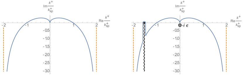
Figure 4: Left panel shows the steepest descent contour for the $k^{+}$ integral. Vertical dashed lines denote the asymptotics of the steepest descent contour. The right panel shows a sample contour which may result from trying to distort the $k^{+}$ integration contour from going along the real axis to the steepest descent contour (see text).

The right panel of Fig. 4 illustrates what happens if one tries to deform the real axis contour into the steepest descent one in the presence of singularities in the complex $k^{+}$ plane. In that plot we explicitly show the essential singularity at $k^{+}=-i\epsilon$ in the integrand of Eq. (3.1): one can see that it does not interfere with the integration contour deformation into the steepest descent shape because it lies outside the contour, and, when the contour approaches this singularity, it does so along the positive imaginary axis near the origin, $k^{+}\approx+i\epsilon^{\prime}$. This region of integration is exponentially suppressed as one can see by plugging $k^{+}\approx+i\epsilon^{\prime}$ into the first exponential of Eq. (3.1). Hence we do not need to worry about the singularity at $k^{+}=-i\epsilon$.

In contrast, the branch cuts may possibly interfere with the contour deformation: this is illustrated in the right panel of Fig. 4 by a sample vertical branch cut with the branch point on the real axis. This branch cut is not an accurate representation of the branch cuts of the $k^{+}$ integrand, and is shown here as a toy model to illustrate the possibility that in deforming the integration contour one may have to wrap the contour around a part of the branch cut as well. The corresponding sample integral would look like (cf. Eqs. (3.1) and (46))

$$\int\limits_{-\infty}^{\infty}\frac{dk^{+}}{2\pi}\,\frac{e^{-ik^{+}x_{1}^{-}-i\,\frac{k_{T}^{2}}{2(k^{+}+i\epsilon)}x_{1}^{+}}}{2(k^{+}+i\epsilon)\,\sqrt{k^{+}-k^{+}_{br}+i\epsilon}}$$ (48)

with $k^{+}_{br}-i\epsilon$ the branch point near the real axis, as shown in the right panel of Fig. 4. (Note again the the branch cut of the square root is chosen along the negative imaginary axis.) Writing

$$k^{+}=k^{+}_{br}-iy$$ (49)

with some real variable $y$ we can approximate the contribution to the integral in Eq. (48) from the part of the contour wrapped around the branch cut by

$$\approx-i\,\int\limits_{0}^{\infty}\frac{dy}{2\pi}\,\frac{e^{-y\,\left(x_{1}^{-}-\frac{k_{T}^{2}}{2(k_{br}^{+})^{2}}\,x_{1}^{+}\right)-ik^{+}_{br}x_{1}^{-}-i\,\frac{k_{T}^{2}}{2k^{+}_{br}}x_{1}^{+}}}{2k^{+}_{br}\,\sqrt{-iy}}=\frac{1-i}{\sqrt{2}}\ \frac{e^{-ik^{+}_{br}x_{1}^{-}-i\,\frac{k_{T}^{2}}{2k^{+}_{br}}x_{1}^{+}}}{4\sqrt{\pi}\,k^{+}_{br}\,\sqrt{x_{1}^{-}-\frac{k_{T}^{2}}{2(k_{br}^{+})^{2}}\,x_{1}^{+}}}.$$ (50)

In the process we have assumed that the branch cut section of the contour is long enough for the upper limit of the $y$ integral in Eq. (50) to be replaced by infinity: this is only valid if $k^{+}_{br}$ is sufficiently far from the saddle point $k^{+}_{sp}$ (and for $|k^{+}_{br}|>|k^{+}_{sp}|$). More specifically, we need $|k^{+}_{br}-k^{+}_{sp}|\gg 1/x_{1}^{-}\sim 1/\tau_{1}$. Since $1/\tau_{1}$ is small for large times $\tau_{1}$, this assumption is justified in most cases.

What we learn from the sample integration in Eqs. (48) and (50) is that the branch cut contribution is dominated by the branch point, $k^{+}=k^{+}_{br}$, with a small region $y\in[0,\sim 1/\tau_{1}]$ near the branch point contributing dominantly to (this part of) the integral.

We are now ready to tackle the full $k^{+}$ and $k^{\prime+}$ integrals in Eq. (3.1). First we need to identify the branch points and branch cuts of the $k^{+}$ and $k^{\prime+}$ integrals. Starting with the $k^{+}$ integral we see that its branch cuts originate in $I_{1}(k^{+}-k_{3}^{+},k^{-}-k_{3}^{-},k_{1T},k_{2T})$ as follows from Eq. (46). Defining

$$\xi=\frac{k^{+}}{k_{3}^{+}}$$ (51)

we conclude that there are four branch points given by

$$\xi_{1,2,3,4}=\frac{1}{2k_{3T}^{2}}\,\left[k_{T}^{2}+k_{3T}^{2}-(k_{1T}\pm k_{2T})^{2}\pm\sqrt{(k_{T}^{2}+k_{3T}^{2}-(k_{1T}\pm k_{2T})^{2})^{2}-4k_{T}^{2}\,k_{3T}^{2}}\right].$$ (52)

(The sign in $(k_{1T}\pm k_{2T})$ is either a plus or a minus simultaneously inside the square root and outside: one cannot have $k_{1T}+k_{2T}$ in one place in the expression and $k_{1T}-k_{2T}$ in another.) These branch points can be real or complex. In the latter case of complex $\xi$ the branch point may contribute to the integral only if $|\mbox{Re}\,\xi|>|k^{+}_{sp}|$, as follows from the contour in Fig. 4. In such case one can easily show that the contribution of the complex-valued branch point in the lower $k^{+}$ half-plane is exponentially suppressed. Since for positive $x_{1}^{-}$ that we are interested in one needs to close the $k^{+}$ integration contour in the lower half-plane, we conclude that we can discard the contributions of the complex-valued branch points.

We are left with the case of real-values branch points $\xi$. Due to the presence of $\theta(-k^{+}\,k_{3}^{+})$ in Eq. (3.1), only the negative real $\xi$ can contribute (otherwise the $k^{+}$ integration never approaches the branch point for it to contribute). A quick analysis of Eq. (52) shows that only two solutions can be real and negative. Let us denote them $\xi_{1}$ and $\xi_{2}$, such that

$$\xi_{1}=\frac{1}{2k_{3T}^{2}}\,\left[k_{T}^{2}+k_{3T}^{2}-(k_{1T}+k_{2T})^{2}+\sqrt{(k_{T}^{2}+k_{3T}^{2}-(k_{1T}+k_{2T})^{2})^{2}-4k_{T}^{2}\,k_{3T}^{2}}\right]$$ (53a)

$$\xi_{2}=\frac{1}{2k_{3T}^{2}}\,\left[k_{T}^{2}+k_{3T}^{2}-(k_{1T}+k_{2T})^{2}-\sqrt{(k_{T}^{2}+k_{3T}^{2}-(k_{1T}+k_{2T})^{2})^{2}-4k_{T}^{2}\,k_{3T}^{2}}\right]$$ (53b)

with $\xi_{2}<\xi_{1}<0$. The corresponding branch point in the $k^{+}$ plane are given by $k^{+}=\xi_{1}\,k_{3}^{+}$ and $k^{+}=\xi_{2}\,k_{3}^{+}$. Note that the branch points of the $k^{\prime+}$ integral are given by the branch points of $I_{1}(k^{\prime+}+k_{3}^{+},k^{\prime-}+k_{3}^{-},k_{1T},k_{2T})$ resulting in $k^{\prime+}=-\xi_{1}\,k_{3}^{+}$ and $k^{\prime+}=-\xi_{2}\,k_{3}^{+}$.

Here we will consider the case of $k_{3}^{+}<0$ (with $k^{+}>0,k^{\prime+}<0$): the $k_{3}^{+}>0$ case can be done by analogy. The branch cuts of the $k^{+}$ and $k^{\prime+}$ integral in the $k_{3}^{+}<0$ case are shown in Fig. 5.

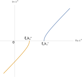
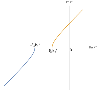
Figure 5: The branch cuts of the integrand in Eq. (3.1) in the complex $k^{+}$ (left panel) and $k^{\prime+}$ (right panel) planes, drawn here for the $k_{3}^{+}<0$ case.

Remembering from the example above that the integrals around our branch cuts are dominated by the branch points, and invoking the argument that the late-time asymptotics is dominated by $k^{\prime+}=-k^{+}$ to avoid rapid oscillations (which would make the function practically zero), we conclude that if the $k^{+}$ integral is wrapped around the branch cut originating at, say, the $\xi_{1}k_{3}^{+}$ branch point, the $k^{\prime+}$ integral must be wrapped around a branch cut originating at the $-\xi_{1}k_{3}^{+}$ branch point. However, as one can see from Fig. 5, while the branch cut starting at $\xi_{1}k_{3}^{+}$ in the $k^{+}$ complex plane lies in the lower half-plane, the branch cut starting at $-\xi_{1}k_{3}^{+}$ in the $k^{\prime+}$ complex plane lies in the upper half-plane. For $x_{1}^{-},x_{2}^{-}>0$ that we are interested in one needs to close the $k^{+}$ and $k^{\prime+}$ contours in the lower half-plane: hence one cannot simultaneously pick up the contributions of the branch cuts originating at $\xi_{1}k_{3}^{+}$ and $-\xi_{1}k_{3}^{+}$ (or at $\xi_{2}k_{3}^{+}$ and $-\xi_{2}k_{3}^{+}$) in the $k^{+}$ and $k^{\prime+}$ integrals. We thus conclude that both the $k^{+}$ and $k^{\prime+}$ integrals can not be dominated by branch cuts.

For a given value of $k_{3}^{+}$, and for $x_{1}^{\pm}\approx x_{2}^{\pm}$, the branch points are either near $|k^{+}_{br}-k^{+}_{sp}|{{}_{\displaystyle{<}}\atop\displaystyle{\sim}}1/\tau$ or far $|k^{+}_{br}-k^{+}_{sp}|\gg 1/\tau$ from the saddle point. The ‘near’ region is small at large $\tau$ and its contribution is suppressed by an extra power of $1/\tau$. Hence the leading contribution to the integral in Eq. (3.1) comes from the ‘far’ region of $|k^{+}_{br}-k^{+}_{sp}|\gg 1/\tau$. In this region branch cuts are clearly separated from the saddle points: if we do not want to have rapidly oscillating exponentials, we can either have the contribution of saddle points in both the $k^{+}$ and $k^{\prime+}$ integrals or of the branch points in both the $k^{+}$ and $k^{\prime+}$ integrals, but due to the separation of branch cuts and saddle points we cannot have a mix where the branch point contributes in one and the saddle point contributes in the other. Since we have just eliminated the contribution of the branch points in both the $k^{+}$ and $k^{\prime+}$ integrals, we are left with the contributions of saddle points only. The saddle point $k^{+}$-integral gives

$$\int\limits_{0}^{\infty}\frac{dk^{+}}{2\pi}\,\frac{e^{-ik^{+}x_{1}^{-}-i\,\frac{k_{T}^{2}}{2(k^{+}+i\epsilon)}x_{1}^{+}}}{2(k^{+}+i\epsilon)}\,I_{1}(k^{+}-k_{3}^{+},k^{-}-k_{3}^{-},k_{1T},k_{2T})\Bigg{|}_{\tau_{1}\to\infty}$$

$$\approx e^{-ik_{T}\,\tau_{1}}\,\frac{1}{2\pi}\,\frac{1-i}{2}\,\sqrt{\frac{\pi}{k_{T}\,\tau_{1}}}\,I_{1}\left(\frac{k_{T}}{\sqrt{2}}\,e^{\eta_{1}}-k_{3}^{+},\frac{k_{T}}{\sqrt{2}}\,e^{-\eta_{1}}-k_{3}^{-},k_{1T},k_{2T}\right)$$ (54)

and

$$\int\limits_{-\infty}^{0}\frac{dk^{\prime+}}{2\pi}\,\frac{e^{-ik^{\prime+}x_{2}^{-}-i\,\frac{k_{T}^{2}}{2(k^{\prime+}+i\epsilon)}x_{2}^{+}}}{2(k^{\prime+}+i\epsilon)}\,I_{1}(k^{\prime+}+k_{3}^{+},k^{\prime-}+k_{3}^{-},k_{1T},k_{2T})\Bigg{|}_{\tau_{2}\to\infty}$$

$$\approx-e^{ik_{T}\,\tau_{2}}\,\frac{1}{2\pi}\,\frac{1+i}{2}\,\sqrt{\frac{\pi}{k_{T}\,\tau_{2}}}\,I_{1}\left(-\frac{k_{T}}{\sqrt{2}}\,e^{\eta_{2}}+k_{3}^{+},-\frac{k_{T}}{\sqrt{2}}\,e^{-\eta_{2}}+k_{3}^{-},k_{1T},k_{2T}\right).$$ (55)

Substituting Eqs. (3.1) and (3.1) into Eq. (3.1) and adding the $k_{3}^{+}>0$ contribution yields

$$\mbox{I+II+II'}\,\bigg{|}_{\tau_{1},\tau_{2}\to\infty}=\frac{\lambda^{2}}{16\pi\sqrt{\tau_{1}\,\tau_{2}}}\,\int\frac{d^{2}k}{(2\pi)^{2}}\frac{d^{2}k_{1}}{(2\pi)^{2}}\frac{d^{2}k_{3}}{(2\pi)^{2}}\,f(k_{1T})\,f(k_{2T})\,e^{i\underline{k}\cdot\underline{x}_{12}}\,\frac{1}{k_{T}}$$

$$\times\,\Bigg{\{}-\int\limits_{-\infty}^{0}\frac{dk_{3}^{+}}{4\pi k_{3}^{+}}\,e^{-ik_{T}\,(\tau_{1}-\tau_{2})}\,I_{1}\left(\frac{k_{T}}{\sqrt{2}}\,e^{\eta_{1}}-k_{3}^{+},\frac{k_{T}}{\sqrt{2}}\,e^{-\eta_{1}}-\frac{\underline{k}_{3}^{2}}{2k_{3}^{+}},k_{1T},k_{2T}\right)$$

$$\times\,I_{1}\left(-\frac{k_{T}}{\sqrt{2}}\,e^{\eta_{2}}+k_{3}^{+},-\frac{k_{T}}{\sqrt{2}}\,e^{-\eta_{2}}+\frac{\underline{k}_{3}^{2}}{2k_{3}^{+}},k_{1T},k_{2T}\right)+\int\limits^{\infty}_{0}\frac{dk_{3}^{+}}{4\pi k_{3}^{+}}\,e^{ik_{T}\,(\tau_{1}-\tau_{2})}$$

$$\times\,I_{1}\left(-\frac{k_{T}}{\sqrt{2}}\,e^{\eta_{1}}-k_{3}^{+},-\frac{k_{T}}{\sqrt{2}}\,e^{-\eta_{1}}-\frac{\underline{k}_{3}^{2}}{2k_{3}^{+}},k_{1T},k_{2T}\right)$$

$$\times\,I_{1}\left(\frac{k_{T}}{\sqrt{2}}\,e^{\eta_{2}}+k_{3}^{+},\frac{k_{T}}{\sqrt{2}}\,e^{-\eta_{2}}+\frac{\underline{k}_{3}^{2}}{2k_{3}^{+}},k_{1T},k_{2T}\right)\Bigg{\}}.$$ (56)

We conclude that

$$\mbox{I+II+II'}\Bigg{|}_{\tau_{1}=\tau_{2}=\tau\to\infty}\sim\frac{1}{\tau},$$ (57)

consistent with free streaming.

3.2 Diagrams III and III’

Our aim now is to calculate diagrams III and III’ from Fig. 3. Following the steps we made for other diagrams, we write

$$\mbox{Diagrams III+III'}=-\lambda^{2}\,\int\frac{d^{4}k}{(2\pi)^{4}}\,e^{-ik\cdot x_{1}}\,\frac{i}{k^{2}+i\epsilon k^{0}}\,\int\frac{d^{4}k^{\prime}}{(2\pi)^{4}}\,e^{-ik^{\prime}\cdot x_{2}}$$ (58)

$$\times\frac{d^{4}k_{1}}{(2\pi)^{4}}\,\frac{d^{4}k_{2}}{(2\pi)^{4}}\,\frac{d^{4}k^{\prime}_{2}}{(2\pi)^{4}}\,\frac{d^{4}k_{3}}{(2\pi)^{4}}\,(2\pi)^{4}\,\delta^{4}(k-k_{1}-k_{2}-k_{3})$$

$$\times\,G^{LO}_{22}(k_{1}+k_{3}-k^{\prime}_{2},k^{\prime})\,G^{LO}_{22}(k_{2},k^{\prime}_{2})\,\frac{i}{k_{1}^{2}+i\epsilon k_{1}^{0}}\,\pi\,\delta(k_{3}^{2})+(x_{1}\leftrightarrow x_{2}).$$

Substituting the leading-order correlators from Eq. (3), integrating out all but one delta-function, and also integrating over $k^{\prime+}$ and $k^{\prime-}$ explicitly yields

$$\mbox{Diagrams III+III'}=\frac{i\,\lambda^{2}}{2}\,\int\limits_{-\infty}^{\infty}\frac{dk^{+}dk^{-}}{(2\pi)^{2}}\,e^{-ik^{+}x_{1}^{-}-ik^{-}x_{1}^{+}}\,\frac{i}{k^{2}+i\epsilon k^{0}}\,J_{0}(k_{T}\,\tau_{2})$$ (59)

$$\times\frac{d^{2}k}{(2\pi)^{2}}\frac{d^{2}k_{1}}{(2\pi)^{2}}\,f(k_{T})\,f(k_{2T})\,e^{i\underline{k}\cdot\underline{x}_{12}}\,\frac{d^{4}k_{3}}{(2\pi)^{4}}\,\pi\,\delta(k_{3}^{2})\,\frac{dk_{1}^{+}dk_{1}^{-}}{(2\pi)^{2}}\,I_{1}(k_{1}^{+}+k_{3}^{+},k_{1}^{-}+k_{3}^{-},k_{2T},k_{T})$$

$$\times\,\frac{i}{k_{1}^{2}+i\epsilon k_{1}^{0}}\,\frac{1}{(k-k_{1}-k_{3})^{2}+i\epsilon(k^{0}-k_{1}^{0}-k_{3}^{0})}+(x_{1}\leftrightarrow x_{2}).$$

Integrating over $k^{-}$ and employing the limit from Eq. (29) one arrives at

$$\mbox{Diagrams III+III'}=\frac{i\,\lambda^{2}}{2}\,\int\limits_{-\infty}^{\infty}\frac{dk^{+}}{2\pi}\,\frac{e^{-ik^{+}x_{1}^{-}-i\frac{k_{T}^{2}}{2(k^{+}+i\epsilon)}x_{1}^{+}}}{2(k^{+}+i\epsilon)}\,J_{0}(k_{T}\,\tau_{2})$$ (60)

$$\times\frac{d^{2}k}{(2\pi)^{2}}\frac{d^{2}k_{1}}{(2\pi)^{2}}\,f(k_{T})\,f(k_{2T})\,e^{i\underline{k}\cdot\underline{x}_{12}}\,\frac{d^{2}k_{3}}{(2\pi)^{2}}\,\frac{dq^{+}dq^{-}}{(2\pi)^{2}}\,I_{1}(q^{+},q^{-},k_{2T},k_{T})\,I_{4}(q^{+},q^{-},k_{3T},k_{1T})$$

$$\times\frac{i}{2(q^{+}-k^{+}-i\epsilon)\,\left(q^{-}-\frac{k_{T}^{2}}{2(k^{+}+i\epsilon)}-i\epsilon\right)-(\underline{k}-\underline{k}_{1}-\underline{k}_{3})^{2}}+(x_{1}\leftrightarrow x_{2}),$$

where we have defined $q^{\pm}\equiv k_{1}^{\pm}+k_{3}^{\pm}$ along with

$$I_{4}(q^{+},q^{-},p_{T},|\underline{q}-\underline{p}|)=\int\limits_{-\infty}^{\infty}\frac{dp^{+}dp^{-}}{(2\pi)^{2}}\,\pi\delta(p^{2})\,G_{R}(q-p).$$ (61)

Consider the integral over $q^{+}$ and $q^{-}$ in Eq. (60):

$$J(k^{+},k_{T},k_{1T},k_{2T},k_{3T})=\int\limits_{-\infty}^{\infty}\,\frac{dq^{+}dq^{-}}{(2\pi)^{2}}\,I_{1}(q^{+},q^{-},k_{2T},k_{T})\,I_{4}(q^{+},q^{-},k_{3T},k_{1T})$$

$$\times\frac{i}{2(q^{+}-k^{+}-i\epsilon)\,\left(q^{-}-\frac{k_{T}^{2}}{2(k^{+}+i\epsilon)}-i\epsilon\right)-(\underline{k}-\underline{k}_{1}-\underline{k}_{3})^{2}}.$$ (62)

This object is boost-invariant. It is a function of several transverse momenta, and of only one longitudinal four-vector component – of $k^{+}$. A boost-invariant object cannot depend on only one $k^{+}$: hence, it must be independent of $k^{+}$, that is,

$$J(k^{+},k_{T},k_{1T},k_{2T},k_{3T})=J(k_{T},k_{1T},k_{2T},k_{3T}).$$ (63)

Eq. (60) becomes

$$\mbox{Diagrams III+III'}=\frac{i\,\lambda^{2}}{2}\,\int\limits_{-\infty}^{\infty}\frac{dk^{+}}{2\pi}\,\frac{e^{-ik^{+}x_{1}^{-}-i\frac{k_{T}^{2}}{2(k^{+}+i\epsilon)}x_{1}^{+}}}{2(k^{+}+i\epsilon)}\,J_{0}(k_{T}\,\tau_{2})$$ (64)

$$\times\frac{d^{2}k}{(2\pi)^{2}}\frac{d^{2}k_{1}}{(2\pi)^{2}}\,f(k_{T})\,f(k_{2T})\,e^{i\underline{k}\cdot\underline{x}_{12}}\,\frac{d^{2}k_{3}}{(2\pi)^{2}}\,J(k_{T},k_{1T},k_{2T},k_{3T})+(x_{1}\leftrightarrow x_{2}).$$

The exact form of $J(k_{T},k_{1T},k_{2T},k_{3T})$ is not important for the late-time asymptotics since now we can integrate over $k^{+}$ exactly, obtaining

$$\mbox{Diagrams III+III'}=\frac{\lambda^{2}}{4}\,\int\frac{d^{2}k}{(2\pi)^{2}}\frac{d^{2}k_{1}}{(2\pi)^{2}}\,J_{0}(k_{T}\,\tau_{1})\,J_{0}(k_{T}\,\tau_{2})$$ (65)

$$\times f(k_{T})\,f(k_{2T})\,e^{i\underline{k}\cdot\underline{x}_{12}}\,\frac{d^{2}k_{3}}{(2\pi)^{2}}\,J(k_{T},k_{1T},k_{2T},k_{3T})+(x_{1}\leftrightarrow x_{2}).$$

We conclude that

$$\mbox{Diagrams III+III'}\Bigg{|}_{\tau_{1}=\tau_{2}=\tau\to\infty}\sim\frac{1}{\tau},$$ (66)

again consistent with free streaming.

3.3 Energy-Momentum Tensor

To cross-check our results let us calculate the longitudinal pressure at $z=0$ (in the massless $\varphi^{4}$ theory at hand):

$$T^{33} =\left\langle(\partial_{z}\varphi)^{2}+{\cal L}\right\rangle\approx\left\langle\frac{1}{2}(\partial_{z}\varphi)^{2}+\frac{1}{2}(\partial_{t}\varphi)^{2}-\frac{1}{2}(\underline{\nabla}\varphi)^{2}\right\rangle$$

$$=-\frac{1}{2}\int\frac{d^{4}k}{(2\pi)^{4}}\,\frac{d^{4}k^{\prime}}{(2\pi)^{4}}\,e^{-i\,(k+k^{\prime})\cdot x}\,\left[k^{z}\,k^{\prime z}+k^{0}\,k^{\prime 0}-\underline{k}\cdot\underline{k}^{\prime}\right]\,G_{22}(k,k^{\prime})$$

$$=-\frac{1}{2}\int\frac{d^{4}k}{(2\pi)^{4}}\,\frac{d^{4}k^{\prime}}{(2\pi)^{4}}\,e^{-i\,(k+k^{\prime})\cdot x}\,\left[k^{+}\,k^{\prime+}+k^{-}\,k^{\prime-}-\underline{k}\cdot\underline{k}^{\prime}\right]\,G_{22}(k,k^{\prime}).$$ (67)

At the leading saddle point $k^{+}_{sp}=\pm\frac{k_{T}}{\sqrt{2}}\,e^{\eta_{1}},\ \ k^{\prime+}_{sp}=\mp\frac{k_{T}}{\sqrt{2}}\,e^{\eta_{2}}$ and at mid-rapidity ($z=0$) the square brackets become

$$\left[k^{+}\,k^{\prime+}+k^{-}\,k^{\prime-}-\underline{k}\cdot\underline{k}^{\prime}\right]\bigg{|}_{z=0}=\left[-\frac{k_{T}^{2}}{2}\,e^{\eta_{1}-\eta_{2}}-\frac{k_{T}^{2}}{2}\,e^{\eta_{2}-\eta_{1}}+k_{T}^{2}\right]\bigg{|}_{\eta_{1}=\eta_{2}=0}=0.$$ (68)

(We have also put $\underline{k}^{\prime}=-\underline{k}$.) We see that the leading saddle point contribution gives the longitudinal pressure

$$P_{L}\big{|}_{\tau\gg\frac{1}{Q_{s}}}=0,$$ (69)

at late time, as characteristic of free streaming.

For completeness, let us calculate the energy density:

$$T^{00} =\left\langle(\partial_{t}\varphi)^{2}-{\cal L}\right\rangle\approx\left\langle\frac{1}{2}(\partial_{z}\varphi)^{2}+\frac{1}{2}(\partial_{t}\varphi)^{2}+\frac{1}{2}(\underline{\nabla}\varphi)^{2}\right\rangle$$

$$=-\frac{1}{2}\int\frac{d^{4}k}{(2\pi)^{4}}\,\frac{d^{4}k^{\prime}}{(2\pi)^{4}}\,e^{-i\,(k+k^{\prime})\cdot x}\,\left[k^{z}\,k^{\prime z}+k^{0}\,k^{\prime 0}+\underline{k}\cdot\underline{k}^{\prime}\right]\,G_{22}(k,k^{\prime})$$

$$=-\frac{1}{2}\int\frac{d^{4}k}{(2\pi)^{4}}\,\frac{d^{4}k^{\prime}}{(2\pi)^{4}}\,e^{-i\,(k+k^{\prime})\cdot x}\,\left[k^{+}\,k^{\prime+}+k^{-}\,k^{\prime-}+\underline{k}\cdot\underline{k}^{\prime}\right]\,G_{22}(k,k^{\prime}).$$ (70)

The saddle points now give (at $z=0$)

$$\left[k^{+}\,k^{\prime+}+k^{-}\,k^{\prime-}+\underline{k}\cdot\underline{k}^{\prime}\right]\bigg{|}_{z=0}=\left[-\frac{k_{T}^{2}}{2}\,e^{\eta_{1}-\eta_{2}}-\frac{k_{T}^{2}}{2}\,e^{\eta_{2}-\eta_{1}}-k_{T}^{2}\right]\bigg{|}_{\eta_{1}=\eta_{2}=0}=-2\,k_{T}^{2},$$ (71)

such that the energy density is

$$\epsilon\big{|}_{\tau\gg\frac{1}{Q_{s}}}\approx-{\underline{\nabla}}_{1}^{2}G_{22}(x_{1},x_{2})\Bigg{|}_{x_{1}=x_{2},\ \tau\gg\frac{1}{Q_{s}}}\sim\frac{1}{\tau},$$ (72)

again in agreement with the free-streaming behavior (16).

Finally, the transverse pressure is

$$T^{11} =\left\langle(\partial_{x}\varphi)^{2}+{\cal L}\right\rangle\approx\left\langle\frac{1}{2}(\partial_{t}\varphi)^{2}-\frac{1}{2}(\partial_{z}\varphi)^{2}+\frac{1}{2}(\partial_{x}\varphi)^{2}-\frac{1}{2}(\partial_{y}\varphi)^{2}\right\rangle$$

$$=-\frac{1}{2}\int\frac{d^{4}k}{(2\pi)^{4}}\,\frac{d^{4}k^{\prime}}{(2\pi)^{4}}\,e^{-i\,(k+k^{\prime})\cdot x}\,\left[k^{0}\,k^{\prime 0}-k^{z}\,k^{\prime z}\right]\,G_{22}(k,k^{\prime})$$

$$=-\frac{1}{2}\int\frac{d^{4}k}{(2\pi)^{4}}\,\frac{d^{4}k^{\prime}}{(2\pi)^{4}}\,e^{-i\,(k+k^{\prime})\cdot x}\,\left[k^{+}\,k^{\prime-}+k^{-}\,k^{\prime+}\right]\,G_{22}(k,k^{\prime}).$$ (73)

Again, at the saddle points at mid-rapidity we get

$$\left[k^{+}\,k^{\prime-}+k^{-}\,k^{\prime+}\right]\bigg{|}_{z=0}=-k_{T}^{2}\,\cosh(\eta_{1}-\eta_{2})\bigg{|}_{\eta_{1}=\eta_{2}=0}=-k_{T}^{2},$$ (74)

and the transverse pressure is

$$P_{T}\big{|}_{\tau\gg\frac{1}{Q_{s}}}\approx-\frac{1}{2}\,{\underline{\nabla}}_{1}^{2}G_{22}(x_{1},x_{2})\Bigg{|}_{x_{1}=x_{2},\ \tau\gg\frac{1}{Q_{s}}}=\frac{1}{2}\,\epsilon\big{|}_{\tau\gg\frac{1}{Q_{s}}}\sim\frac{1}{\tau},$$ (75)

in complete agreement with the free-streaming expectations (16).

4 Two-point correlation function with a single rescattering: Full diagrammatic calculation in the Wigner representation

In this Section we calculate the late-time asymptotics of the correlation function $G_{22}(X,p)$ in the Wigner representation. We start with the calculation of the classical two-point correlation function given by the diagram in Fig. 2. Then, we calculate $G_{22}(X,p)$ due to a single $2\to 2$ rescattering using the diagrams in Fig. 3.

4.1 The asymptotic expansion of the classical correlation function in $1/\tau$

From (3) we have

$$G_{22}^{LO}(X,p) =\int\frac{d^{4}k}{(2\pi)^{4}}e^{-ik\cdot X}G_{22}^{LO}(k/2+p,k/2-p)$$

$$=-f(p_{T})\int\frac{dk^{+}dk^{-}}{(2\pi)^{2}}e^{-ik^{+}X^{-}-ik^{-}X^{+}}G_{R}(k/2-p)G_{R}(k/2+p)$$ (76)

with $k_{T}=0$. One can integrate out $k^{-}$ by closing the integration contour downward and picking up the residues of the poles in the lower half-plane. There are two poles in the lower half-plane

$$k^{-}=k_{1p}^{-}\equiv\frac{2p_{\perp}^{2}}{k^{+}-2p^{+}}+2p^{-}\qquad\text{and}\qquad k^{-}=k_{2p}^{-}\equiv\frac{2p_{\perp}^{2}}{k^{+}+2p^{+}}-2p^{-},$$ (77)

and their residues yield

$$G_{22}^{LO}(X,p) =-if(p_{T})\int\frac{dk^{+}}{2\pi}\left.\frac{e^{-i(k^{-}X^{+}+k^{+}X^{-})}}{{p^{-}\left[\left(k^{+}\right)^{2}-\frac{2p^{+}p^{2}}{p^{-}}\right]}}\right|_{k^{-}=k_{2p}^{-}}^{k^{-}=k_{1p}^{-}}$$

$$=-if(p_{T})\int\frac{dk^{+}}{2\pi}\left\{\frac{e^{-i\left[2X^{+}\left(\frac{p_{T}^{2}}{k^{+}-2p^{+}}+p^{-}\right)+k^{+}X^{-}\right]}}{{p^{-}\left[\left(k^{+}\right)^{2}-\frac{2p^{+}p^{2}}{p^{-}}\right]}}\right.$$

$$\left.-\frac{e^{-i\left[\frac{2X^{+}p_{T}^{2}}{k^{+}+2p^{+}}+k^{+}X^{-}-2p^{-}X^{+}\right]}}{{p^{-}\left[\left(k^{+}\right)^{2}-\frac{2p^{+}p^{2}}{p^{-}}\right]}}\right\}$$ (78)

with the understanding that the $k^{+}$ integration contour is located infinitesimally above the real axis.

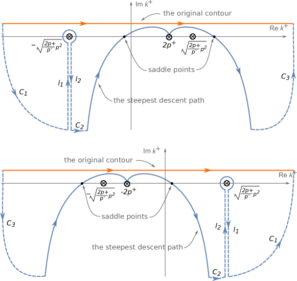
Figure 6: Deformation of integration contours for the $1^{st}$ (top) and $2^{nd}$ (bottom) terms on the right-hand side of (78). In each figure, the original integration contour is a horizontal line infinitesimally above the real axis. It is deformed so that it continues along the steepest descent path. The contributions from integrating over $l_{1}$ and $l_{2}$ cancel with each other and the contributions from the arcs, $C_{1}$, $C_{2}$ and $C_{3}$, vanish as their radius goes to $\infty$.

In this paper we are only interested in the asymptotic behavior of $G_{22}(X,p)$ at large $\tau$. For this goal, we evaluate the two terms on the right-hand side of (78) separately. The integrand of each term has a steepest descent path passing through two saddle points respectively located at

$$k^{+}=2p^{+}\pm p_{T}\sqrt{\frac{2X^{+}}{X^{-}}}\qquad\text{for the first term},$$ (79)

and

$$k^{+}=-2p^{+}\pm p_{T}\sqrt{\frac{2X^{+}}{X^{-}}}\qquad\text{for the second term}.$$ (80)

As illustrated in Fig. 6, we deform the integration contours for these two integrals so that they continue along the steepest descent paths. Each term has two other poles at

$$k^{+}=\pm 2p^{+}\sqrt{\frac{p^{2}}{2p^{+}p^{-}}}.$$ (81)

Here, one only needs to consider the case with $\frac{p^{2}}{2p^{+}p^{-}}>0$ since the residues of these poles will be exponentially suppressed at large $\tau$ otherwise. The contour deformation may involve passing through these poles. If this is the case, one needs to pick up the contribution from their residues. By integrating over the deformed contours one can easily pick up the contributions from the residues of the poles (81) and from the steepest descent paths.

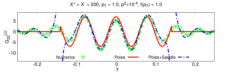
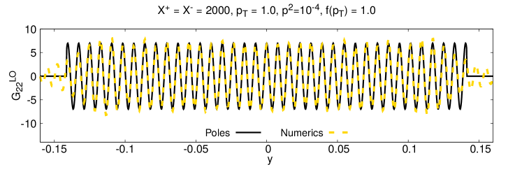
Figure 7: Comparison with the numerical calculation of $G_{22}^{LO}(X,p)$. The top figure shows our analytical result in (85) (Poles), the sum of (85) and (86) (Poles+Saddle) and our numerical result (Numerics) at $X^{+}=X^{-}=200$. The bottom figure shows our result from poles (Poles) and our numerical result (Numerics) at $X^{+}=X^{-}=2000$. (The units are arbitrary.)

The residues of the poles yield a contribution with an amplitude of $O(\tau^{0})$ at large $\tau$. It is easy to see that the integrand on the right hand side of (78) as a whole is not singular at the points in (81). That is, the residues of the two terms at the same pole cancel with each other. Therefore, we only need to take into account the case when the deformed contours for the two terms pass through different poles: $k^{+}=2p^{+}\sqrt{\frac{p^{2}}{2p^{+}p^{-}}}$ for the first term and $k^{+}=-2p^{+}\sqrt{\frac{p^{2}}{2p^{+}p^{-}}}$ for the second term. As illustrated in Fig. 6, for $p^{+}>0$ this requires

$$2p^{+}+p_{T}\sqrt{\frac{2X^{+}}{X^{-}}}>2p^{+}\sqrt{\frac{p^{2}}{2p^{+}p^{-}}}>2p^{+}-p_{T}\sqrt{\frac{2X^{+}}{X^{-}}}>-2p^{+}\sqrt{\frac{p^{2}}{2p^{+}p^{-}}},$$ (82)

which is equivalent to

$$\tau>\frac{p_{T}}{2|p^{+}p^{-}|}|p^{+}X^{-}+p^{-}X^{+}|.$$ (83)

Similarly, for $p^{+}<0$ this requires

$$-2p^{+}\sqrt{\frac{p^{2}}{2p^{+}p^{-}}}>2p^{+}+p_{T}\sqrt{\frac{2X^{+}}{X^{-}}}>2p^{+}\sqrt{\frac{p^{2}}{2p^{+}p^{-}}}>2p^{+}-p_{T}\sqrt{\frac{2X^{+}}{X^{-}}},$$ (84)

which is also equivalent to (83). By combining the results for both $p^{+}>0$ and $p^{+}<0$, we obtain the following contribution to $G_{22}^{LO}(X,p)$ from the residues of the poles

Poles $$=\frac{\cos\left(2\sqrt{\frac{p^{2}}{2p^{+}p^{-}}}\left(p^{+}X^{-}-p^{-}X^{+}\right)\right)}{2p^{-}p^{+}\sqrt{\frac{p^{2}}{2p^{-}p^{+}}}}$$

$$\times\theta\left(\frac{p^{2}}{2p^{-}p^{+}}\right)\theta\left(\tau-\frac{p_{T}}{2|p^{+}p^{-}|}\left|p^{+}X^{-}+p^{-}X^{+}\right|\right)\,f(p_{T}).$$ (85)

As shown in Fig. 7, the above result agrees very well with our numerical result of $G_{22}^{LO}(X,p)$ at large $\tau$.

The integration over the steepest descent paths gives a contribution with an amplitude of $O(\tau^{-\frac{1}{2}})$ at large $\tau$. Such a contribution comes from the integration over a small region in the vicinity of each saddle point in (79) and (80). One only needs to expand the exponent of the exponential function in a Taylor series around each saddle point up to the second order and replace $k^{+}$ in the rest part of the integrand by the saddle point value. By doing this and integrating out $k^{+}$, we get

$$\text{Saddle Points}=\frac{1}{2}\left(\frac{1}{2\pi p_{T}\tau}\right)^{\frac{1}{2}}$$ (86)

$$\times\left[\frac{\sin\left(2\left(p^{-}X^{+}+p^{+}X^{-}-p_{T}\tau\right)\right)-\cos\left(2\left(p^{-}X^{+}+p^{+}X^{-}-p_{T}\tau\right)\right)}{\frac{p_{T}}{\tau}\left(p^{-}X^{+}+p^{+}X^{-}\right)-2p^{-}p^{+}}\right.$$

$$\left.\qquad+\frac{\sin\left(2\left(p^{-}X^{+}+p^{+}X^{-}+p_{T}\tau\right)\right)+\cos\left(2\left(p^{-}X^{+}+p^{+}X^{-}+p_{T}\tau\right)\right)}{\frac{p_{T}}{\tau}\left(p^{-}X^{+}+p^{+}X^{-}\right)+2p^{-}p^{+}}\right]\,f(p_{T}).$$

As shown in the figure on the top of Fig. 7, the above result is indeed needed for us to understand the $\tau$ dependence of $G_{22}^{LO}(X,p)$ at an intermediate large time except when the saddle points coincide with poles. This coincidence explains the divergence between the exact numerical results and the dash-dotted line in the top panel of Fig. 7. Our exact numerical results in Fig. 7 show that $G_{22}^{LO}(X,p)$ is well behaved in these regions. Hence, these regions should not be important for calculating any observables involving $G_{22}(X,p)$ and we do not need to construct a separate analytical expression for these regions. As one can see from the lower panel of Fig. 7, these regions become progressively less important at later times.

In Ref. WuKovchegov we find that the classical gluon two-point function is

$$\left.G_{22}^{a\mu,b\nu}(X,p)\right|_{\tau\to\infty}\propto\delta^{ab}\sum\limits_{\lambda=\pm}\epsilon_{\lambda}^{\mu}(p)\epsilon_{\lambda}^{*\nu}(p)\frac{1}{\tau}\delta(p^{2})\delta(y-\eta)$$ (87)

with

$$y\equiv\frac{1}{2}\ln\frac{p^{+}}{p^{-}},\qquad\eta\equiv\frac{1}{2}\ln\frac{X^{+}}{X^{-}}.$$ (88)

If we use

$$\lim\limits_{\tau\to\infty}\left[\tau\frac{\cos(\tau yx)}{x}\right]=2\pi\delta(y)\delta(x^{2}),$$ (89)

we obtain from Eq. (85)

$$\left.G_{22}(X,p)\right|_{\tau\to\infty}=\frac{\pi}{\tau p_{T}}\delta\left(p^{2}\right)\delta(y-\eta)\theta\left(\frac{p^{2}}{2p^{+}p^{-}}\right)\theta(1-\cosh(y-\eta))\,f(p_{T}).$$ (90)

for our scalar correlator. In order to get the correct coefficient of the above equation, we write

$$\left.G_{22}(X,p)\right|_{\tau\to\infty}=c_{\theta}\frac{\pi}{\tau p_{T}}\delta\left(p^{2}\right)\delta(y-\eta)\,f(p_{T}),$$ (91)

and fix $c_{\theta}$ by integrating out $p^{\pm}$ and matching it to that by integrating (85) over $p^{\pm}$. It is convenient to define $\nu\equiv p^{2}=2p^{+}p^{-}-p_{T}^{2}$ and $y=\frac{1}{2}\ln\left|\frac{p^{+}}{p^{-}}\right|$. In terms of these two variables, Eq. (85) reduces to, for $p^{+}p^{-}>0$,

$$\mbox{Poles}=\frac{\cos\left(2\tau\sqrt{{\nu}}\sinh(y-\eta)\right)}{\sqrt{\nu(\nu+p_{T}^{2})}}\theta\left(\nu-p_{T}^{2}\sinh^{2}(y-\eta)\right)\,f(p_{T}),$$ (92)

and, for $p^{+}p^{-}<0$,

$$\mbox{Poles}=-\frac{\cos\left(2\tau\sqrt{{-\nu}}\cosh(y-\eta)\right)}{\sqrt{\nu(\nu+p_{T}^{2})}}\theta\left(-\nu-p_{T}^{2}\cosh^{2}(y-\eta)\right)\,f(p_{T}).$$ (93)

Accordingly, we have

$$\int\limits_{-\infty}^{\infty}dp^{+}dp^{-}\mbox{Poles}=\left(\int\limits_{-k_{T}^{2}}^{+\infty}d\nu\int\limits_{-\infty}^{+\infty}dy+\int\limits_{-\infty}^{-k_{T}^{2}}d\nu\int\limits_{-\infty}^{+\infty}dy\right)\mbox{Poles}\equiv n_{1}+n_{2}$$ (94)

with only Eq. (92) contributing to $n_{1}$ and only Eq. (93) contributing to $n_{2}$. After changing variables to $\hat{s}=\sinh(y-\eta)$ and $\hat{\nu}=\sqrt{p^{2}}/p_{T}$, we have

$$n_{1}=2\int\limits_{0}^{\infty}d\hat{\nu}\int\limits_{0}^{\infty}d\hat{s}\frac{\cos(2\tau p_{T}\hat{\nu}\hat{s})}{\sqrt{(\hat{\nu}^{2}+1)(\hat{s}^{2}+1)}}\,f(p_{T}).$$ (95)

We only need to obtain the large $\tau$ asymptotics. At large $\tau$, the predominant contribution to the above integral comes from the region $\hat{\nu}\approx 0$ and $\hat{s}\approx 0$. So one can not take either $\tau\hat{\nu}$ or $\tau\hat{s}$ as the large expansion parameter. We do the following trick: we rotate the integration contour of, say $\hat{s}$, to go along the positive imaginary axis. Then the $[0,i]$ region of integration does not contribute to the real part of the integral. We get

$$n_{1} =2\text{Re}\int\limits_{0}^{\infty}d\hat{\nu}\int\limits_{0}^{\infty}d\hat{s}\frac{e^{i2\tau p_{T}\hat{\nu}\hat{s}}}{\sqrt{(\hat{\nu}^{2}+1)(\hat{s}^{2}+1)}}\,f(p_{T})=2\int\limits_{0}^{\infty}d\hat{\nu}\int\limits_{1}^{\infty}d\hat{s}\frac{e^{-2\tau p_{T}\hat{\nu}\hat{s}}}{\sqrt{(\hat{\nu}^{2}+1)(\hat{s}^{2}-1)}}\,f(p_{T})$$

$$\approx 2\int\limits_{1}^{\infty}\frac{d\hat{s}}{2\tau p_{T}\hat{s}\sqrt{\hat{s}^{2}-1}}\,f(p_{T})=\frac{\pi}{2\,\tau\,p_{T}}\,f(p_{T}).$$ (96)

Similarly, by changing variables to $\hat{s}=\cosh(y-\eta)$ and $\hat{\nu}=\sqrt{-p^{2}}/p_{T}$, we have

$$n_{2} =-2\!\int\limits_{1}^{\infty}d\hat{\nu}\int\limits_{1}^{\infty}d\hat{s}\frac{\cos(2\tau p_{T}\hat{\nu}\hat{s})}{\sqrt{(\hat{\nu}^{2}-1)(\hat{s}^{2}-1)}}\,f(p_{T})\approx-2\text{Re}\!\int\limits_{1}^{\infty}d\hat{\nu}\frac{e^{i2\tau p_{T}\hat{\nu}-i\frac{\pi}{4}}}{\sqrt{(\hat{\nu}^{2}-1)}}\frac{i}{2}\left(\frac{\pi}{\tau p_{T}\hat{\nu}}\right)^{\frac{1}{2}}\!f(p_{T})$$

$$\approx\frac{\pi}{2\tau p_{T}}\sin(2\tau p_{T})\,f(p_{T}).$$ (97)

One can simply discard $n_{2}$ since it is a highly oscillatory function at large $\tau$. From $n_{1}$ we obtain $c_{\theta}=1/2$ and

$$\left.G_{22}(X,p)\right|_{\tau\to\infty}=\frac{\pi}{2\tau p_{T}}\delta(y-\eta)\delta(p^{2})\,f(p_{T}).$$ (98)

4.2 $G_{22}(X,p)$ from a singe rescattering

Let us evaluate the late time asymptotics of each diagram in Fig. 3 using the same techniques as for $G_{22}^{LO}(X,p)$ in the previous subsection.

4.2.1 Diagram I

From (3.1), we have in Wigner representation

$$\mbox{Diagram I}= -\frac{\lambda^{2}}{2}\int\frac{d^{2}k_{1}}{(2\pi)^{2}}\,f(k_{1T})\,f(k_{2T})\int\frac{d^{4}k_{3}}{(2\pi)^{4}}\,\pi\,\delta(k_{3}^{2})\int\limits_{-\infty}^{\infty}\frac{dk^{+}\,dk^{-}}{(2\pi)^{2}}$$

$$\times\,e^{-ik^{+}X^{-}-ik^{-}X^{+}}\,G_{R}\left(\frac{k}{2}+p\right)G_{R}\left(\frac{k}{2}-p\right)\Pi(k^{+},k^{-}),$$ (99)

where

$$\Pi(k^{+},k^{-}) \equiv I_{1}\left(\frac{k^{+}}{2}+p^{+}-k_{3}^{+},\frac{k^{-}}{2}+p^{-}-k_{3}^{-},k_{1T},k_{2T}\right)\,$$

$$\times I_{1}\left(\frac{k^{+}}{2}-p^{+}+k_{3}^{+},\frac{k^{-}}{2}-p^{-}+k_{3}^{-},k_{1T},k_{2T}\right)$$ (100)

with $\underline{k}=0$ and $\underline{k}_{2}=\underline{p}-\underline{k}_{1}-\underline{k}_{3}$. The integration contours for $k^{+}$ and $k^{-}$ are understood to be located infinitesimally above the real axis of the $k^{\pm}$ plane and we shall drop all the $i\epsilon$’s in both $G_{R}$ and $I_{1}$.

Figure 8: Integration contour for $k^{-}$. In the integration over $k^{-}$ in (4.2.1), the integration contour is deformed in order to pick up the predominant contribution at late times from the regions around singular points (poles and branch points). The portions of the contour giving vanishing or canceling contributions are indicated by the dashed lines.

In order to calculate the late-time asymptotics, we first need to identify all the critical points including poles, branch points and saddle points. For $k^{-}$, the integrand on the right hand of (4.2.1) has two poles given by (77) and 4 branch points at

$$k^{-}=2\left[\frac{\left(k_{1T}\pm k_{2T}\right){}^{2}}{k^{+}+2k_{3}^{+}-2p^{+}}-k_{3}^{-}+p^{-}\right]$$ (101)

and

$$k^{-}=2\left[\frac{\left(k_{1T}\pm k_{2T}\right){}^{2}}{k^{+}-2k_{3}^{+}+2p^{+}}+k_{3}^{-}-p^{-}\right].$$ (102)

As shown in Fig. 8, we deform the integration contour such that it goes around the two poles and continues along the branch cuts. Then, $k^{-}$ integration is given by the residues of the two poles and the integration along the branch cuts, as indicated by the solid lines in Fig. 8. At late times, the poles give a contribution proportional to $\tau^{0}$ while the branch cuts yield a contribution proportional to $\tau^{-\frac{1}{2}}$. Hence, we only keep the contribution from the residues of the poles. As a result, we get

$$\mbox{Diagram I}= -\frac{\lambda^{2}}{2p^{-}}\int\frac{d^{2}k_{1}}{(2\pi)^{2}}\,f(k_{1T})\,f(k_{2T})\int\frac{d^{4}k_{3}}{(2\pi)^{4}}\,\pi\,\delta(k_{3}^{2})\int\limits_{-\infty}^{\infty}\frac{dk^{+}\,}{2\pi}$$

$$\times\,\frac{i}{\left(k^{+}\right)^{2}-\frac{2p^{+}}{p^{-}}p^{2}}\left[\left.e^{-ik^{+}X^{-}-ik^{-}X^{+}}\,\Pi(k^{+},k^{-})\right]\right|^{k^{-}=\frac{2p_{T}^{2}}{k^{+}-2p^{+}}+2p^{-}}_{k^{-}=\frac{2p_{T}^{2}}{k^{+}+2p^{+}}-2p^{-}}.$$ (103)

For $k^{+}$, the integrand on the right hand side of (4.2.1) has poles given by (81). It also has saddle points and branch cuts. Since they only give a contribution proportional to $\tau^{-\frac{1}{2}}$, we only need to keep the contribution from the residues of the poles. The calculation is straightforward and similar to the leading-order case of Sec. 4.1. We obtain

$$\mbox{Diagram I}= \frac{\lambda^{2}}{4p^{+}p^{-}\sqrt{\frac{p^{2}}{2p^{+}p^{-}}}}~{}\text{Re}\Bigg{[}\int\frac{d^{2}k_{1}}{(2\pi)^{2}}\,f(k_{1T})\,f(k_{2T})\int\frac{d^{4}k_{3}}{(2\pi)^{4}}\,\pi\,\delta(k_{3}^{2})$$

$$\times\theta\left(\frac{p^{2}}{2p^{-}p^{+}}\right)\theta\left(\tau-\frac{p_{T}}{2|p^{+}p^{-}|}\left|p^{+}X^{-}+p^{-}X^{+}\right|\right)\,$$

$$\times e^{2i\sqrt{\frac{p^{2}}{2p^{+}p^{-}}}\left(p^{+}X^{-}-p^{-}X^{+}\right)}\Pi\left(-2p^{+}\sqrt{\frac{p^{2}}{2p^{+}p^{-}}},2p^{-}\sqrt{\frac{p^{2}}{2p^{+}p^{-}}}\right)\Bigg{]}\,,$$ (104)

where we have used the identity

$$I_{1}(-q^{+},-q^{-},k_{1T},k_{2T})=I_{1}^{*}(q^{+},q^{-},k_{1T},k_{2T})$$ (105)

to shorten the expression by taking the real part. Based on the same calculation as for (98) we obtain

$$\left.\mbox{Diagram I}\right|_{\tau\to\infty} =\frac{\lambda^{2}}{2}\int\frac{d^{2}k_{1}}{(2\pi)^{2}}\,f(k_{1T})\,f(k_{2T})\int\frac{d^{4}k_{3}}{(2\pi)^{4}}\,\pi\,\delta(k_{3}^{2})\,$$

$$\times\frac{\pi}{2\,\tau\,p_{T}}\delta(y-\eta)\delta(p^{2})\left|I_{1}\left(p^{+}-k_{3}^{+},p^{-}-k_{3}^{-},k_{1T},k_{2T}\right)\right|^{2}.$$ (106)

4.2.2 Diagrams II and II’

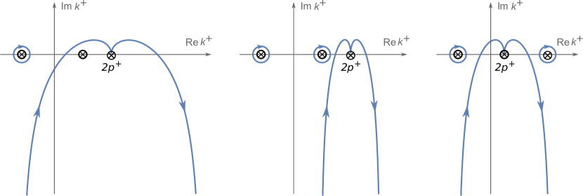
Figure 9: Relative positions of poles with respect to the steepest descent path. Here, we assume that $p^{+}>0$ and that the two poles are located at $k^{+}=\pm 2p^{+}\sqrt{\frac{p^{2}}{2p^{+}p^{-}}}$. These 3 figures show all the possible cases when one needs to keep the residues of the poles in the $k^{+}$ integration in (4.2.2).

From (3.1) we have in Wigner representation

$$\mbox{Diagrams II+II'}= -\frac{\lambda^{2}}{2}\int\frac{d^{2}k_{1}}{(2\pi)^{2}}\,f(k_{1T})\,f(k_{2T})\int\frac{d^{4}k_{3}}{(2\pi)^{4}}\int\limits_{-\infty}^{\infty}\frac{dk^{+}\,dk^{-}}{(2\pi)^{2}}\,e^{-ik^{+}X^{-}-ik^{-}X^{+}}\,$$

$$\times\left[\,\pi\delta\left(\left(\frac{k}{2}+p\right)^{2}\right)G_{R}\left(\frac{k}{2}-p\right)G_{A}(k_{3})\right.\,$$

$$+\left.\,G_{R}\left(\frac{k}{2}+p\right)\pi\delta\left(\left(\frac{k}{2}-p\right)^{2}\right)G_{R}(k_{3})\right]\Pi(k^{+},k^{-}),$$ (107)

with $\underline{k}=0$ and $\underline{k}_{2}=\underline{p}-\underline{k}_{1}-\underline{k}_{3}$. By integrating out $k^{-}$ we obtain

$$\mbox{Diagrams II+II'}= -\frac{\lambda^{2}}{4p^{-}}\int\frac{d^{2}k_{1}}{(2\pi)^{2}}\,f(k_{1T})\,f(k_{2T})\int\frac{d^{4}k_{3}}{(2\pi)^{4}}\int\limits_{-\infty}^{\infty}\frac{dk^{+}}{2\pi}\frac{i}{\left(k^{+}\right)^{2}-\frac{2p^{+}}{p^{-}}p^{2}}\,$$

$$\times\left[\,e^{-ik^{+}X^{-}-ik_{1p}^{-}X^{+}}~{}\mbox{Sign}\left(k^{+}-2p^{+}\right)G_{R}(k_{3})\Pi(k^{+},k_{1p}^{-})\right.\,$$

$$-\left.e^{-ik^{+}X^{-}-ik_{2p}^{-}X^{+}}~{}\mbox{Sign}\left(k^{+}+2p^{+}\right)G_{A}(k_{3})\Pi(k^{+},k_{2p}^{-})\right]$$ (108)

with $k_{1p}^{-}$ and $k_{2p}^{-}$ given in (77). By using Eq. (105) one can show that the second term on the right hand side of (4.2.2) gives a contribution which is the complex conjugate of the first term.

We only evaluate the late time asymptotics from diagrams II and II’. The integrand on the right hand side of (4.2.2) has poles, saddle points and branch points. As before, we deform the integration contour so that it wraps around poles, continues along the steepest descent path and goes along the branch cuts. Then, at large $\tau$ we only need to pick up the contribution from the poles. Since there is no obvious cancellation between the residues of the poles for the two terms in (4.2.2), we need to keep the contributions from all the poles which are in the way of the contour deformation. As shown in Fig. 9, there are 3 possible cases when we need to keep the residues of poles. Correspondingly, they yield

Diagrams II+II’ $$=-\frac{\lambda^{2}}{8p^{+}p^{-}\sqrt{\frac{p^{2}}{2p^{+}p^{-}}}}\theta\left(\frac{p^{2}}{2p^{-}p^{+}}\right)\text{Sign}(p^{+})\int\frac{d^{2}k_{1}}{(2\pi)^{2}}\frac{d^{4}k_{3}}{(2\pi)^{4}}\,f(k_{1T})\,f(k_{2T})$$

$$\times~{}\text{Re}~{}\Bigg{\{}G_{R}(k_{3})\,\left[\,\theta\left(\tau-\frac{p_{T}}{2|p^{+}p^{-}|}\left|p^{+}X^{-}+p^{-}X^{+}\right|\right)\right.$$

$$\left.+2i\,\theta\left(\frac{2|p^{+}|}{p_{T}}\left(1-\sqrt{\frac{p^{2}}{2p^{+}p^{-}}}\right)-\sqrt{\frac{2X^{+}}{X^{-}}}\right)\text{Im}\right.\,$$

$$\left.+2\,\theta\left(\frac{2|p^{+}|}{p_{T}}\left(\sqrt{\frac{p^{2}}{2p^{+}p^{-}}}-1\right)-\sqrt{\frac{2X^{+}}{X^{-}}}\right)\text{Re}\right]\,$$

$$\times e^{2i\sqrt{\frac{p^{2}}{2p^{+}p^{-}}}\left(p^{+}X^{-}-p^{-}X^{+}\right)}\Pi\left(-2p^{+}\sqrt{\frac{p^{2}}{2p^{+}p^{-}}},2p^{-}\sqrt{\frac{p^{2}}{2p^{+}p^{-}}}\right)\Bigg{\}},$$ (109)

where Re and Im in the curly brackets act on everything to their right. Taking the large-$\tau$ limit using Eq. (89) we see that only the cosine part of the exponential contributes, putting $y=\eta$ and $p^{2}=0$ while approaching this latter limit from the side where $p^{2}/(2p^{+}p^{-})>0$. This way, the second and third terms in the square brackets vanish. To take the real part in the first term we employ the Cutkosky rules Cutkosky:1960sp , which prescribe the replacement

$$\frac{1}{k_{3}^{2}+i\epsilon k_{3}^{+}}\to-2\pi i\,\delta(k_{3}^{2})\,\mbox{Sign}(k_{3}^{+}).$$ (110)

This gives

$$\left.\mbox{Diagrams II+II'}\right|_{\tau\to\infty}=-\frac{\lambda^{2}}{2}\text{Sign}(p^{+})\int\frac{d^{2}k_{1}}{(2\pi)^{2}}\frac{d^{4}k_{3}}{(2\pi)^{4}}\,f(k_{1T})\,f(k_{2T})$$

$$\times~{}\text{Sign}(k_{3}^{+})\pi\delta(k_{3}^{2})\frac{\pi}{2\,\tau\,p_{T}}\delta(y-\eta)\delta(p^{2})\left|I_{1}\left(p^{+}-k_{3}^{+},p^{-}-k_{3}^{-},k_{1T},k_{2T}\right)\right|^{2}.$$ (111)

Adding this result to diagram I leads to a cancellation similar to that observed in Eq. (3.1). In the end we obtain

$$\left.\mbox{Diagrams I+ II+II'}\right|_{\tau\to\infty}=\frac{\pi\lambda^{2}}{2\tau}\delta(y-\eta)\delta(p^{2})\int\frac{d^{2}k_{1}}{(2\pi)^{2}}\frac{d^{4}k_{3}}{(2\pi)^{4}}\,f(k_{1T})\,f(k_{2T})$$

$$\qquad\times~{}\theta(-k_{3}^{+}p^{+})\,\pi\delta(k_{3}^{2})\left|I_{1}\left(p^{+}-k_{3}^{+},p^{-}-k_{3}^{-},k_{1T},k_{2T}\right)\right|^{2}.$$ (112)

4.2.3 Diagrams III and III’

Let us now evaluate diagrams III and III’ from Fig. 3. Similar to that in coordinate space, we have, now in Wigner representation

$$\mbox{Diagrams III+III'}=-\lambda^{2}\int\limits_{-\infty}^{\infty}\frac{dk^{+}dk^{-}}{(2\pi)^{2}}e^{-ik^{+}X^{-}-ik^{-}X^{+}}G_{R}\left(\frac{k}{2}+p\right)G_{R}\left(\frac{k}{2}-p\right)$$

$$\times\int\frac{d^{4}k_{1}}{(2\pi)^{4}}\frac{d^{4}k_{3}}{(2\pi)^{4}}\,f(p_{T})\,f(k_{2T})\left[G_{R}\left(\frac{k}{2}+p-k_{1}-k_{3}\right)+G_{R}\left(\frac{k}{2}-p-k_{1}-k_{3}\right)\right]$$

$$\times G_{R}(k_{1})\pi\delta(k_{3}^{2})I_{1}(k_{1}^{+}+k_{3}^{+},k_{1}^{-}+k_{3}^{-},k_{2T},p_{T}).$$ (113)

It is easy to see that diagram III’ is a complex conjugate of diagram III. By employing this fact and (29) at large $\tau$, we can write

$$\mbox{Diagrams III+III'}=-\frac{2\lambda^{2}}{p^{-}}\mbox{Re}\int\frac{d^{2}k_{1}}{(2\pi)^{2}}\frac{d^{2}k_{3}}{(2\pi)^{2}}\,f(p_{T})\,f(k_{2T})\frac{dq^{+}dq^{-}}{(2\pi)^{2}}I_{1}(q^{+},q^{-},k_{2T},p_{T})$$

$$\times\left.\int\limits_{-\infty}^{\infty}\frac{dk^{+}}{2\pi}\frac{ie^{-ik^{+}X^{-}-ik^{-}X^{+}}}{(k^{+})^{2}-\frac{2p^{+}}{p^{-}}p^{2}}I_{4}(q^{+},q^{-},k_{3T},k_{1T})G_{R}\left(\frac{k}{2}+p-q\right)\right|^{k^{-}=k^{-}_{1p}}_{k^{-}=k^{-}_{2p}}$$

$$=-\frac{2\lambda^{2}}{p^{-}}\mbox{Re}\int\frac{d^{2}k_{1}}{(2\pi)^{2}}\frac{d^{2}k_{3}}{(2\pi)^{2}}\,f(p_{T})\,f(k_{2T})\int\limits_{-\infty}^{\infty}\frac{dk^{+}}{2\pi}\frac{i}{(k^{+})^{2}-\frac{2p^{+}}{p^{-}}p^{2}}$$

$$\times\left[\left.e^{-ik^{+}X^{-}-ik^{-}X^{+}}J\left(\frac{k^{+}}{2}-p^{+},p_{T},k_{1T},k_{2T},k_{3T}\right)\right]\right|^{k^{-}=k^{-}_{1p}}_{k^{-}=k^{-}_{2p}},$$ (114)

where we put $\underline{q}=\underline{k}_{1}+\underline{k}_{3}$. Using (63) leads to

$$\mbox{Diagrams III+III'}=-\frac{2\lambda^{2}}{p^{-}}\mbox{Re}\int\frac{d^{2}k_{1}}{(2\pi)^{2}}\frac{d^{2}k_{3}}{(2\pi)^{2}}\,f(p_{T})\,f(k_{2T})\int\limits_{-\infty}^{\infty}\frac{dk^{+}}{2\pi}\frac{i}{(k^{+})^{2}-\frac{2p^{+}}{p^{-}}p^{2}}$$

$$\times\left[\left.e^{-ik^{+}X^{-}-ik^{-}X^{+}}J\left(p_{T},k_{1T},k_{2T},k_{3T}\right)\right]\right|^{k^{-}=k^{-}_{1p}}_{k^{-}=k^{-}_{2p}}.$$ (115)

At the end we have

$$\mbox{Diagrams III+III'}=\frac{2\lambda^{2}}{p^{-}}\mbox{Re}\int\frac{d^{2}k_{1}}{(2\pi)^{2}}\frac{d^{2}k_{3}}{(2\pi)^{2}}\,f(p_{T})\,f(k_{2T})J\left(p_{T},k_{1T},k_{2T},k_{3T}\right)\theta\left(\frac{p^{2}}{2p^{-}p^{+}}\right)$$

$$\times\theta\left(\tau-\frac{p_{T}}{2|p^{+}p^{-}|}\left|p^{+}X^{-}+p^{-}X^{+}\right|\right)\frac{\cos\left(2\sqrt{\frac{p^{2}}{2p^{+}p^{-}}}\left(p^{+}X^{-}-p^{-}X^{+}\right)\right)}{2p^{-}p^{+}\sqrt{\frac{p^{2}}{2p^{-}p^{+}}}}.$$ (116)

That is, at late times

$$\mbox{Diagrams III+III'}\Bigg{|}_{\tau\to\infty}\sim\frac{1}{\tau}\delta(p^{2})\delta(\eta-y).$$ (117)

Combining (4.2.2) and (117) we conclude once again that the late-time asymptotics of the rescattering diagrams in Fig. 3, calculated this time in Wigner representation, is consistent with free streaming.

5 Conclusions and Outlook

In the first paper WuKovchegov of this ‘duplex’ we have outlined the way to apply the Schwinger–Keldysh formalism to ultrarelativistic heavy ion collisions, thus setting the stage for the calculation of time-dependent observables, such as the energy-momentum tensor, in the collisions. As the first application of this technique, in WuKovchegov we have tried to re-derive the Boltzmann equation for the medium produced in heavy ion collisions by considering a single $2\to 2$ rescattering correction to the classical gluon fields of the MV model. We have employed the “on-shell” approximation for the propagators that one usually employs in deriving the kinetic theory. The result was dependent on the time-ordering assumptions outlined above in Sec. 1: kinetic theory emerged under the assumption (i), while free-streaming was obtained if assumption (ii) was employed.

In this paper we have used the formalism set up in WuKovchegov to re-do the calculation of the $2\to 2$ rescattering correction to the classical fields without using the “on-shell” approximation for the propagators and without assuming a specific time-ordering of the interaction time versus the measurement time. Performing the calculation twice, both in momentum space (Sec. 3) and in the Wigner representation (Sec. 4), we have arrived at the results consistent with free streaming (16). We have thus found no evidence for the applicability of the kinetic theory (employing the Boltzmann equation taken with the full collision term) to the perturbative description of heavy ion collisions.

Our perturbative calculations of the energy-momentum tensor are consistent with the conclusion reached in Kovchegov:2005ss , where it was argued that the energy density of the produced weakly-coupled medium is given by

$$\epsilon(\tau,\eta,\underline{b})\bigg{|}_{\tau\gg 1/Q_{s}}\,\approx\,\frac{1}{\tau}\,\int d^{2}k_{T}\ k_{T}\ \frac{dN}{d^{2}k_{T}\,d\eta\,d^{2}b_{T}}$$ (118)

at any order in perturbation theory. In the scenario advocated in Kovchegov:2005ss , higher-order perturbative corrections would only modify the gluon multiplicity distribution $dN/d^{2}k_{T}\,d\eta\,d^{2}b_{T}$ and the saturation scale $Q_{s}$, leaving the $\tau$-dependence of Eq. (118) unchanged.

In the future we hope that the formalism we have presented in WuKovchegov will be useful for calculations of time-dependent heavy ion observables. In particular it can be used to cross-check (and possibly challenge) the conclusion in (118) by explicit perturbative calculations. Our own cross-check presented above did not show any deviations from (118) and disagreed with kinetic theory. Perhaps other thermalization scenarios may fare better in challenging Eq. (118). Indeed calculations of higher-order perturbative corrections to the classical gluon field contributions to heavy ion observables appear to be very complicated. In our minds, however, such calculations would present a necessary theoretical test for any thermalization scenario. If, for instance, a given thermalization proposal claims to resum a certain $\tau$-dependent parameter to all orders, then this parameter should manifest itself in some lower-order perturbative calculation. In other words, one needs to prove that the resummation parameter exists. If the explicit calculation fails to confirm that the resummation parameter exists, the thermalization scenario in question should be discarded. If the equation (118) does turn out to be exact in the perturbation theory, then calculation of higher-order corrections would improve our knowledge of gluon multiplicity and energy density, which would also be very useful. We hope the formalism and calculations presented in WuKovchegov and in this paper lay the groundwork for future cross-checks of thermalization scenarios and will facilitate calculations of heavy-ion observables in the years to come.

Appendix A $I_{1}$ Calculation

The goal of this Appendix is to calculate

$$I_{1}(q^{+},q^{-},k_{T},p_{T})=\int\limits_{-\infty}^{\infty}\frac{dk^{+}dk^{-}}{(2\pi)^{2}}\,G_{R}(k)\,G_{R}(q-k)$$ (119)

with

$${\underline{p}}={\underline{q}}-{\underline{k}}.$$ (120)

Taking $G_{R}$ from Eq. (21) and integrating (119) over $k^{-}$ we get

$$I_{1}=\int\limits_{-\infty}^{\infty}\frac{dk^{+}}{2\pi}\frac{i}{2(q^{+}-k^{+})(2q^{-}k^{+}-k_{T}^{2})-2k^{+}\,p_{T}^{2}+i\,\epsilon\,k^{+}(q^{+}-k^{+})}.$$ (121)

The poles of the integrand are given by

$$k^{+}_{1,2}=\frac{1}{-4q^{-}}\left[p_{T}^{2}-k_{T}^{2}-2q^{+}q^{-}\pm\sqrt{D}\right]$$ (122)

with the discriminant

$$D \equiv[(k_{T}-p_{T})^{2}-2q^{+}q^{-}][(k_{T}+p_{T})^{2}-2q^{+}q^{-}]$$

$$=(k_{T}^{2}+p_{T}^{2}-2q^{+}q^{-})^{2}-4\,k_{T}^{2}\,p_{T}^{2}.$$ (123)

Using $k^{+}_{1,2}$ we rewrite Eq. (121) as

$$I_{1}=\frac{1}{-4q^{-}}\int\limits_{-\infty}^{\infty}\frac{dk^{+}}{2\pi}\frac{i}{(k^{+}-k_{1}^{+}+i\epsilon r_{1})\,(k^{+}-k_{2}^{+}+i\epsilon r_{2})},$$ (124)

where the coefficients $r_{1},r_{2}$ have to be determined by matching the linear in $\epsilon$ terms in the denominators of (124) and (121) at the poles $k^{+}=k_{1}^{+}$ and $k^{+}=k_{2}^{+}$ respectively. This gives

$$-4q^{-}(k_{1}^{+}-k_{2}^{+})\,r_{1}=k_{1}^{+}\,(q^{+}-k_{1}^{+}),$$ (125a)

$$-4q^{-}(k_{2}^{+}-k_{1}^{+})\,r_{2}=k_{2}^{+}\,(q^{+}-k_{2}^{+}).$$ (125b)

Multiplying Eqs. (125) after a little algebra we arrive at

$$-(4q^{-})^{2}\,(k_{1}^{+}-k_{2}^{+})^{2}\,r_{1}\,r_{2}=k_{T}^{2}\,p_{T}^{2}\,\left(\frac{q^{+}}{2\,q^{-}}\right)^{2}.$$ (126)

We are now ready to integrate Eq. (124) over $k^{+}$. To do so we need to consider two cases:

• Case I: $D<0$. In this case $k_{1}^{+}$ and $k_{2}^{+}$ have non-zero (and non-infinitesimal) imaginary parts, and the $i\epsilon$ terms along with the values of $r_{1}$ and $r_{2}$ in Eq. (124) are not important. Integrating Eq. (124) over $k^{+}$ we obtain

  $$I_{1}\Big{|}_{D<0}=-\frac{i}{2\sqrt{|D|}}\,\mbox{Sign}(q^{-})=-\frac{i}{2\sqrt{|D|}}\,\mbox{Sign}(q^{+}).$$ (127)

  (We have used the fact that $q^{+}q^{-}>0$ if $D<0$.)

• Case II: $D>0$. Now $k_{1}^{+}$ and $k_{2}^{+}$ are real. This, along with Eq. (126) implies that $r_{1}r_{2}<0$. Integrating Eq. (124) over $k^{+}$ yields

  $$I_{1}\Big{|}_{D>0}=\frac{\mbox{Sign}(r_{1})}{2\sqrt{D}}.$$ (128)

  Employing Eq. (125a) we get Sign$(r_{1})$ = Sign$[k_{1}^{+}\,(q^{+}-k_{1}^{+})]$. The $D>0$ case can be realized in the following two ways:

  $$(a)~{}(k_{T}+p_{T})^{2}-2q^{+}q^{-}<0\qquad\text{or}\qquad(b)~{}(k_{T}-p_{T})^{2}-2q^{+}q^{-}>0.$$ (129)

  For the case (a), after some algebra involving Eqs. (122) and (A) one can show that Sign$(r_{1})=+1$. For the case (b), one can similarly show that Sign$(r_{1})=-1$. We conclude that

  $$I_{1}\Big{|}_{D>0}=\frac{\theta\left(2q^{+}q^{-}-(k_{T}+p_{T})^{2}\right)-\theta\left((k_{T}-p_{T})^{2}-2q^{+}q^{-}\right)}{2\sqrt{D}}.$$ (130)

By combining the above cases I and II, we have

$$I_{1}=\frac{\theta\left(2q^{+}q^{-}-(k_{T}+p_{T})^{2}\right)-\theta\left((k_{T}-p_{T})^{2}-2q^{+}q^{-}\right)-i\theta(-D)\,\mbox{Sign}~{}(q^{\pm})}{2\sqrt{|D|}}.$$ (131)

In order to perform integrations using the complex plane, it is desirable to rewrite $I_{1}$ without $\theta$-functions, since the latter are hard to analytically continue into the whole complex plane. This is achieved by re-writing Eq. (131) as

$$I_{1} =\frac{1}{4(q^{-}+i\epsilon)\left[q^{+}+i\epsilon-\frac{(k_{T}+p_{T})^{2}}{2(q^{-}+i\epsilon)}\right]^{\frac{1}{2}}\ \left[q^{+}+i\epsilon-\frac{(k_{T}-p_{T})^{2}}{2(q^{-}+i\epsilon)}\right]^{\frac{1}{2}}}$$

$$=\frac{1}{4(q^{+}+i\epsilon)\left[q^{-}+i\epsilon-\frac{(k_{T}+p_{T})^{2}}{2(q^{+}+i\epsilon)}\right]^{\frac{1}{2}}\ \left[q^{-}-\frac{(k_{T}-p_{T})^{2}}{2(q^{+}+i\epsilon)}\right]^{\frac{1}{2}}}.$$ (132)

The $i\epsilon$ regulators are needed for the “standard” branch cut of the square root running along the negative real axis. If we choose the branch cut of the square root to run along the negative imaginary axis, one can neglect these $i\epsilon$’s, arriving at the Eq. (46) in the main text.

References

- (1) J. M. Maldacena, The large N limit of superconformal field theories and supergravity, Adv. Theor. Math. Phys. 2 (1998) 231–252, [hep-th/9711200].
- (2) E. Witten, Anti-de Sitter space and holography, Adv. Theor. Math. Phys. 2 (1998) 253–291, [hep-th/9802150].
- (3) S. S. Gubser, S. S. Pufu and A. Yarom, Entropy production in collisions of gravitational shock waves and of heavy ions, Phys. Rev. D78 (2008) 066014, [0805.1551].
- (4) S. Lin and E. Shuryak, Grazing Collisions of Gravitational Shock Waves and Entropy Production in Heavy Ion Collision, Phys. Rev. D79 (2009) 124015, [0902.1508].
- (5) Y. V. Kovchegov and S. Lin, Toward Thermalization in Heavy Ion Collisions at Strong Coupling, JHEP 1003 (2010) 057, [0911.4707].
- (6) P. M. Chesler and L. G. Yaffe, Boost invariant flow, black hole formation, and far-from-equilibrium dynamics in supersymmetric Yang-Mills theory, Phys.Rev. D82 (2010) 026006, [0906.4426].
- (7) P. M. Chesler and L. G. Yaffe, Holography and colliding gravitational shock waves in asymptotically AdS5 spacetime, Phys.Rev.Lett. 106 (2011) 021601, [1011.3562].
- (8) R. Baier, A. H. Mueller, D. Schiff and D. T. Son, ’Bottom up’ thermalization in heavy ion collisions, Phys. Lett. B502 (2001) 51–58, [hep-ph/0009237].
- (9) L. D. McLerran and R. Venugopalan, Computing quark and gluon distribution functions for very large nuclei, Phys. Rev. D49 (1994) 2233–2241, [hep-ph/9309289].
- (10) L. D. McLerran and R. Venugopalan, Gluon distribution functions for very large nuclei at small transverse momentum, Phys. Rev. D49 (1994) 3352–3355, [hep-ph/9311205].
- (11) L. D. McLerran and R. Venugopalan, Green’s functions in the color field of a large nucleus, Phys. Rev. D50 (1994) 2225–2233, [hep-ph/9402335].
- (12) A. Krasnitz and R. Venugopalan, Non-perturbative computation of gluon mini-jet production in nuclear collisions at very high energies, Nucl. Phys. B557 (1999) 237, [hep-ph/9809433].
- (13) A. Krasnitz and R. Venugopalan, The initial energy density of gluons produced in very high energy nuclear collisions, Phys. Rev. Lett. 84 (2000) 4309–4312, [hep-ph/9909203].
- (14) A. Krasnitz, Y. Nara and R. Venugopalan, Probing a color glass condensate in high energy heavy ion collisions, Braz. J. Phys. 33 (2003) 223–230.
- (15) T. Lappi, Production of gluons in the classical field model for heavy ion collisions, Phys. Rev. C67 (2003) 054903, [hep-ph/0303076].
- (16) P. B. Arnold, J. Lenaghan and G. D. Moore, QCD plasma instabilities and bottom up thermalization, JHEP 08 (2003) 002, [hep-ph/0307325].
- (17) P. Arnold and J. Lenaghan, The abelianization of QCD plasma instabilities, Phys. Rev. D70 (2004) 114007, [hep-ph/0408052].
- (18) P. Arnold, J. Lenaghan, G. D. Moore and L. G. Yaffe, Apparent thermalization due to plasma instabilities in quark gluon plasma, Phys. Rev. Lett. 94 (2005) 072302, [nucl-th/0409068].
- (19) A. Rebhan, P. Romatschke and M. Strickland, Hard-loop dynamics of non-Abelian plasma instabilities, Phys. Rev. Lett. 94 (2005) 102303, [hep-ph/0412016].
- (20) P. Romatschke and R. Venugopalan, The unstable glasma, Phys. Rev. D74 (2006) 045011, [hep-ph/0605045].
- (21) J. Berges, K. Boguslavski, S. Schlichting and R. Venugopalan, Universal attractor in a highly occupied non-Abelian plasma, Phys. Rev. D89 (2014) 114007, [1311.3005].
- (22) T. Epelbaum and F. Gelis, Pressure isotropization in high energy heavy ion collisions, Phys. Rev. Lett. 111 (2013) 232301, [1307.2214].
- (23) T. Epelbaum, F. Gelis and B. Wu, Nonrenormalizability of the classical statistical approximation, Phys. Rev. D90 (2014) 065029, [1402.0115].
- (24) T. Epelbaum, F. Gelis, N. Tanji and B. Wu, Properties of the Boltzmann equation in the classical approximation, Phys. Rev. D90 (2014) 125032, [1409.0701].
- (25) A. H. Mueller and D. T. Son, On the Equivalence between the Boltzmann equation and classical field theory at large occupation numbers, Phys. Lett. B582 (2004) 279–287, [hep-ph/0212198].
- (26) P. B. Arnold, G. D. Moore and L. G. Yaffe, Effective kinetic theory for high temperature gauge theories, JHEP 01 (2003) 030, [hep-ph/0209353].
- (27) A. Kurkela and Y. Zhu, Isotropization and hydrodynamization in weakly coupled heavy-ion collisions, Phys. Rev. Lett. 115 (2015) 182301, [1506.06647].
- (28) L. V. Gribov, E. M. Levin and M. G. Ryskin, Semihard Processes in QCD, Phys. Rept. 100 (1983) 1–150.
- (29) E. Iancu and R. Venugopalan, The color glass condensate and high energy scattering in QCD, hep-ph/0303204.
- (30) H. Weigert, Evolution at small : The Color Glass Condensate, Prog. Part. Nucl. Phys. 55 (2005) 461–565, [hep-ph/0501087].
- (31) J. Jalilian-Marian and Y. V. Kovchegov, Saturation physics and deuteron gold collisions at RHIC, Prog. Part. Nucl. Phys. 56 (2006) 104–231, [hep-ph/0505052].
- (32) F. Gelis, E. Iancu, J. Jalilian-Marian and R. Venugopalan, The Color Glass Condensate, Ann.Rev.Nucl.Part.Sci. 60 (2010) 463–489, [1002.0333].
- (33) J. L. Albacete and C. Marquet, Gluon saturation and initial conditions for relativistic heavy ion collisions, Prog.Part.Nucl.Phys. 76 (2014) 1–42, [1401.4866].
- (34) Y. V. Kovchegov and E. Levin, Quantum Chromodynamics at High Energy. Cambridge University Press, 2012.
- (35) A. H. Mueller, Small x Behavior and Parton Saturation: A QCD Model, Nucl. Phys. B335 (1990) 115.
- (36) I. Balitsky, Operator expansion for high-energy scattering, Nucl. Phys. B463 (1996) 99–160, [hep-ph/9509348].
- (37) I. Balitsky, Factorization and high-energy effective action, Phys. Rev. D60 (1999) 014020, [hep-ph/9812311].
- (38) Y. V. Kovchegov, Small-x structure function of a nucleus including multiple pomeron exchanges, Phys. Rev. D60 (1999) 034008, [hep-ph/9901281].
- (39) Y. V. Kovchegov, Unitarization of the BFKL pomeron on a nucleus, Phys. Rev. D61 (2000) 074018, [hep-ph/9905214].
- (40) J. Jalilian-Marian, A. Kovner and H. Weigert, The Wilson renormalization group for low x physics: Gluon evolution at finite parton density, Phys. Rev. D59 (1998) 014015, [hep-ph/9709432].
- (41) J. Jalilian-Marian, A. Kovner, A. Leonidov and H. Weigert, The Wilson renormalization group for low x physics: Towards the high density regime, Phys. Rev. D59 (1998) 014014, [hep-ph/9706377].
- (42) E. Iancu, A. Leonidov and L. D. McLerran, The renormalization group equation for the color glass condensate, Phys. Lett. B510 (2001) 133–144.
- (43) E. Iancu, A. Leonidov and L. D. McLerran, Nonlinear gluon evolution in the color glass condensate. I, Nucl. Phys. A692 (2001) 583–645, [hep-ph/0011241].
- (44) I. Balitsky, Scattering of shock waves in QCD, Phys. Rev. D70 (2004) 114030, [hep-ph/0409314].
- (45) G. A. Chirilli, Y. V. Kovchegov and D. E. Wertepny, Classical Gluon Production Amplitude for Nucleus-Nucleus Collisions: First Saturation Correction in the Projectile, JHEP 03 (2015) 015, [1501.03106].
- (46) A. Kovner, L. D. McLerran and H. Weigert, Gluon production at high transverse momentum in the mclerran-venugopalan model of nuclear structure functions, Phys. Rev. D52 (1995) 3809–3814, [hep-ph/9505320].
- (47) A. Kovner, L. D. McLerran and H. Weigert, Gluon production from nonAbelian Weizsacker-Williams fields in nucleus-nucleus collisions, Phys. Rev. D52 (1995) 6231–6237, [hep-ph/9502289].
- (48) Y. V. Kovchegov and D. H. Rischke, Classical gluon radiation in ultrarelativistic nucleus nucleus collisions, Phys. Rev. C56 (1997) 1084–1094, [hep-ph/9704201].
- (49) Y. V. Kovchegov and A. H. Mueller, Gluon production in current nucleus and nucleon nucleus collisions in a quasi-classical approximation, Nucl. Phys. B529 (1998) 451–479, [hep-ph/9802440].
- (50) A. Dumitru and L. D. McLerran, How protons shatter colored glass, Nucl. Phys. A700 (2002) 492–508, [hep-ph/0105268].
- (51) F. Gelis, T. Lappi and R. Venugopalan, High energy factorization in nucleus-nucleus collisions, Phys.Rev. D78 (2008) 054019, [0804.2630].
- (52) F. Gelis, T. Lappi and R. Venugopalan, High energy factorization in nucleus-nucleus collisions. II. Multigluon correlations, Phys.Rev. D78 (2008) 054020, [0807.1306].
- (53) Y. V. Kovchegov, Can thermalization in heavy ion collisions be described by QCD diagrams?, Nucl. Phys. A762 (2005) 298–325, [hep-ph/0503038].
- (54) Y. V. Kovchegov, Thoughts on non-perturbative thermalization and jet quenching in heavy ion collisions, Nucl. Phys. A764 (2006) 476–497, [hep-ph/0507134].
- (55) B. Wu and Y. V. Kovchegov, “Time-Dependent Observables in Heavy Ion Collisions I: Setting up the Formalism.” in preparation, 2017.
- (56) F. Gelis and R. Venugopalan, Particle production in field theories coupled to strong external sources, Nucl. Phys. A776 (2006) 135–171, [hep-ph/0601209].
- (57) T. Lappi, Energy density of the glasma, Phys. Lett. B643 (2006) 11–16, [hep-ph/0606207].
- (58) T. Epelbaum, F. Gelis, S. Jeon, G. Moore and B. Wu, Kinetic theory of a longitudinally expanding system of scalar particles, JHEP 09 (2015) 117, [1506.05580].
- (59) G. P. Lepage and S. J. Brodsky, Exclusive processes in perturbative quantum chromodynamics, Phys. Rev. D22 (1980) 2157.
- (60) R. Cutkosky, Singularities and discontinuities of Feynman amplitudes, J.Math.Phys. 1 (1960) 429–433.