Time-Dependent Observables in Heavy Ion Collisions I: Setting up the Formalism

Abstract

We adapt the Schwinger-Keldysh formalism to study heavy-ion collisions in perturbative QCD. Employing the formalism, we calculate the two-point gluon correlation function $G_{22}^{a\mu,b\nu}$ due to the lowest-order classical gluon fields in the McLerran-Venugopalan model of heavy ion collisions and observe an interesting transition from the classical fields to the quasi-particle picture at later times. Motivated by this observation, we push the formalism to higher orders in the coupling and calculate the contribution to $G_{22}^{a\mu,b\nu}$ coming from the diagrams representing a single rescattering between two of the produced gluons. We assume that the two gluons go on mass shell both before and after the rescattering. The result of our calculation depends on the ordering between the proper time of the rescattering $\tau_{Z}$ and the proper time $\tau$ when the gluon distribution is measured. For (i) $\tau_{Z}\gg 1/Q_{s}$ and $\tau-\tau_{Z}\gg 1/Q_{s}$ (with $Q_{s}$ the saturation scale) we obtain the same results as from the Boltzmann equation. For (ii) $\tau-\tau_{Z}\gg\tau_{Z}\gg 1/Q_{s}$ we end up with a result very different from kinetic theory and consistent with a picture of “free-streaming” particles. Due to the approximations made, our calculation is too coarse to indicate whether the ordering (i) or (ii) is the correct one: to resolve this controversy, we shall present a detailed diagrammatic calculation of the rescattering correction in the $\varphi^{4}$ theory in the second paper of this duplex.

1 Introduction

The ultimate goal of heavy-ion collision is to produce and study quark-gluon plasma (QGP). QGP is believed to be the primordial matter in our early universe after the Big bang and before the formation of nucleons. Heavy-ion collision experiments at RHIC and LHC provide us a golden opportunity to study such a new form of matter. The detectors only measure the properties of the system at a very late time $\tau\sim 10^{15}~{}\text{fm}/c$ after the collision. QGP is believed to exist only in the first 10-20 fm/$c$ after the collision: for the majority of the remaining time the system reduces to a multitude of hadrons free-streaming towards the detector. The entire evolution history of bulk matter in the first 10-20 fm/$c$ can be studied only by comparing theoretical calculations to the experimental data at roughly $10^{15}~{}\text{fm}/c$. However, a consistent first-principles QCD formalism allowing to study the system from the very beginning of the collision to a moderate late time is still missing.

Hydrodynamic models could give a good description of the collective behavior seen in the experimental data (see Heinz:2013th for a recent review). Hydrodynamics can be taken as an effective theory of the underlying quantum field theory near (local) thermal equilibrium Jeon:1995zm . Since bulk matter in heavy-ion collisions is far from thermal equilibrium at the very early stage, hydrodynamics breaks down at those early times. In practice, hydrodynamic models are switched on at some initial time $\tau_{0}$ with the initial condition provided by other theoretical studies. In order to study the early stage of the collision one needs to employ the underlying field theory.

At the very early stage of a collision, a large number of saturated gluons are believed to be freed from the two nuclear wave functions (see Gelis:2010nm ; KovchegovLevin for a comprehensive review). In this case the classical Yang-Mills theory applies. It has been extensively studied in McLerran:1993ni ; McLerran:1993ka ; McLerran:1994vd ; Kovchegov:1996ty ; Ayala:1996hx ; Kovchegov:1997ke ; Krasnitz:1998ns ; Krasnitz:1999wc ; Krasnitz:2003nv ; Lappi:2003bi ; Kovchegov:2005ss ; Berges:2013fga ; Gelis:2013rba . However, this approach can only give a highly anisotropized energy-momentum tensor with the ratio of the longitudinal to transverse pressures $P_{L}/P_{T}$ approaching zero at later times Krasnitz:1998ns ; Krasnitz:1999wc ; Krasnitz:2003nv ; Kovchegov:2005ss ; Berges:2013fga . Early pressure isotropization has been observed if certain types of vacuum quantum fluctuations are included in the classical field simulation Epelbaum:2013waa ; Gelis:2013rba . In this case one has to deal with the dependence of the medium energy-momentum tensor on the lattice spacing Gelis:2013rba ; Berges:2013lsa . This is a consequence of the non-renormalizability of the classical field approach with vacuum quantum fluctuations Epelbaum:2014yja ; Epelbaum:2014mfa .

The Boltzmann equation has also been broadly used in heavy-ion collisions. It can be derived from two-point Green functions in quantum theory using the so-called quasi-particle approximation near thermal equilibrium Kadanoff ; Chou:1984es ; Calzetta:1986cq ; Blaizot:2001nr ; Arnold:2002zm . The transition from classical fields to quasi-particles is expected to occur at $\tau\sim 1/Q_{s}$ with $Q_{s}$ the saturation momentum of the colliding nuclei Baier:2000sb . Then, a parametric estimate using the quasi-particle picture gives a bottom-up scenario for the system to establish thermal equilibrium Baier:2000sb . This picture has recently been confirmed by numerical solutions of the Boltzmann equation Kurkela:2015qoa . One of the intriguing questions about the Boltzmann equation is when it starts to apply to heavy-ion collisions since the derivation of this equation from quantum field theory has mostly been done for the systems near thermal equilibrium. The conventional understanding is that when the gluon density $f$ is less than $1/g^{2}$ (with $g$ the QCD coupling), both the Boltzmann equation and classical field approximation apply Mueller:2002gd . However, this argument is based on the so-called quasi-particle approximation. It is of great interest to understand whether and how such a transition occurs in the collision process.

The Schwinger-Keldysh formalism or the close-time path formalism was first invented by Schwinger Schwinger:1960qe and Keldysh Keldysh:1964ud . It gives a unified description of equilibrium and non-equilibrium systems in quantum field theory Chou:1984es . This formalism has been used to study thermal equilibrium systems in thermal field theory Landsman:1986uw ; Bellac:2011kqa . It has also been used to study non-equilibrium systems by resumming two-particle-irreducible (2PI) or n-particle-irreducible (nPI) diagrams Cornwall:1974vz ; Calzetta:1986cq ; Berges:2004pu . The interested reader is referred to Berges:2004yj ; Calzetta:1986cq for a comprehensive review for the nPI effective theories. A 2PI non-Abelian gauge theory would be of great interest to heavy-ion physics. However, the truncated 2PI effective action leads to gauge-dependent results for most observables Carrington:2003ut . In high-energy nuclear physics, the Schwinger-Keldysh formalism has been employed to resum leading $\ln\frac{1}{x}$ terms with $x$ the energy fraction into the color charge density functionals describing the colliding nuclei Gelis:2008rw ; Gelis:2008ad ; Jeon:2013zga . However, contributions beyond the leading $\ln\frac{1}{x}$ have not been evaluated: such contributions could be important for the evolution of the system at late times.

The main purpose of this paper is to adapt the Schwinger-Keldysh formalism to study heavy-ion collisions in a perturbative approach. This approach is obviously gauge invariant. This paper is organized as follows. We first give a brief review of this formalism and derive the Feynman rules for perturbative calculations in Sec. 2. In Sec. 3 we recalculate the gluon two-point function by using the lowest-order classical gluon fields of the McLerran-Venugopalan (MV) model McLerran:1993ni ; McLerran:1993ka ; McLerran:1994vd in the light-cone gauge. Based on this calculation, we show explicitly how quasi-particles emerge from classical fields. In Sec. 4 we study the contribution from a $2\to 2$ rescattering of these quasi-particles to the two-point Green function. That is, we study the rescattering of two particles produced by the classical gluon fields, assuming that the particles go on mass-shell both before and after the collision. The result of this calculation appears to depend on the ordering between the rescattering proper time $\tau_{Z}$ and the proper time $\tau$ when the gluon is measured. For (i) $\tau_{Z}\gg 1/Q_{s}$ and $\tau-\tau_{Z}\gg 1/Q_{s}$ our diagrammatic approach leads to the same answer as that obtained by solving the Boltzmann equation. However, as we show in Sec. 5, for (ii) $\tau-\tau_{Z}\gg\tau_{Z}\gg 1/Q_{s}$ the result is consistent with free-streaming gluons in the final state, and is very different from the solution of the Boltzmann equation. Further discussion of the physics behind the differences of cases (i) and (ii) is presented in Sec. 6. The resolution of the question of whether the assumption (i) or assumption (ii) is correct is done in the second paper KovchegovWu of this duplex.

2 The Schwinger-Keldysh formalism for heavy ion collisions

In this Section, we shall give a detailed description of the formalism used in our calculation. We adapt the Schwinger-Keldysh formalism Schwinger:1960qe ; Keldysh:1964ud to describe the collision of two particles composed of a finite number of constituents. Following Mueller:1989st ; McLerran:1993ni ; McLerran:1993ka ; Kovchegov:1996ty , the two colliding nuclei are taken to consist respectively of $A_{1}$ and $A_{2}$ constituent quarks at $t=-\infty$, each valence quark representing a nucleon. Classical gluon fields resum the parameters $\alpha_{s}^{2}\,A_{1}^{1/3}$ and $\alpha_{s}^{2}\,A_{2}^{1/3}$ to all orders Kovchegov:1997pc : in the actual calculations below we assume these parameters to be small, which would allow us to expand in them perturbatively.

2.1 The Schwinger-Keldysh formalism in perturbation theory

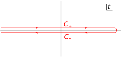
Figure 1: The Schwinger-Keldysh contour in the complex time plane.

We formulate our problem in terms of the density matrix $\rho$, which can be written in terms of the wave functions of the two colliding particles $\Psi_{1}$ and $\Psi_{2}$ before the collision

$$\rho(t_{i})=\left|\Psi_{1},\Psi_{2}\right>\left<\Psi_{1},\Psi_{2}\right|.$$ (1)

In the Schrödinger picture, the expectation value of any operator $O$ is given by

$$O(t)=\mathrm{Tr}\left[O_{s}e^{-iH(t-t_{i})}\rho_{s}(t_{i})e^{iH(t-t_{i})}\right].$$ (2)

In order to perform perturbative calculations, we shall use the interaction picture by separating $H$ into a free part $H_{0}$ and an interaction part $H_{I}$. Let us denote the operator in the interaction picture by

$$O_{I}(t)=e^{iH_{0}t}O_{s}e^{-iH_{0}t}$$ (3)

and the time evolution operator by

$$U(t,t_{i})=e^{iH_{0}t}e^{-iH(t-t_{i})}e^{-iH_{0}t_{i}}=Te^{i\int d^{4}x\mathcal{L}_{I}}$$ (4)

where $\mathcal{L}_{I}$ is the interaction Lagrangian corresponding to $H_{I}$. From (2), it is easy to show that

$$O(t)=\mathrm{Tr}\left[O_{I}(t)U(t,t_{i})\rho_{I}(t_{i})U^{\dagger}(t,t_{i})\right],$$ (5)

It is convenient to define the time ordering $T_{\mathcal{C}}$ along the Schwinger-Keldysh contour $\mathcal{C}=\mathcal{C}_{+}\bigcup\mathcal{C}_{-}$. As illustrated in Fig. 1, the contour $\mathcal{C}$ runs from $-\infty$ to $+\infty$ and back to $-\infty$. On $\mathcal{C}$, the time ordering $T_{\mathcal{C}}$ can be defined in the same way as the normal time ordering by replacing the $\theta$ function by Niemi:1983nf

$$\theta_{\mathcal{C}}(t_{1}-t_{2})=\left\{\begin{array}[]{ll}\theta(t_{1}-t_{2})&\text{if }t_{1},t_{2}\in\mathcal{C}_{+},\\ 0&\text{if }t_{1}\in\mathcal{C}_{+},t_{2}\in\mathcal{C}_{-},\\ 1&\text{if }t_{2}\in\mathcal{C}_{+},t_{1}\in\mathcal{C}_{-},\\ \theta(t_{2}-t_{1})&\text{if }t_{1},t_{2}\in\mathcal{C}_{-}.\end{array}\right.$$ (10)

Accordingly, one can write

$$O(t)=\mathrm{Tr}\left[T_{\mathcal{C}}\left\{O_{I}(t)e^{i\int_{\mathcal{C}}d^{4}x\mathcal{L}_{I}}\rho_{I}(t_{i})\right\}\right]$$ (11)

with $\int_{\mathcal{C}}d^{4}x\equiv\int_{\mathcal{C}}dx^{0}\int d^{3}{\bf x}$.

Given any free field $\Phi$, one can define the free propagator

$$G^{(0)}(x_{1},x_{2}) \equiv\left<0|T_{\mathcal{C}}[\Phi(x_{1})\Phi(x_{2})]|0\right>$$

$$=\theta_{\mathcal{C}}(t_{1}-t_{2})[\Phi_{p}(x_{1}),\Phi_{n}(x_{2})]+(-1)^{F}\theta_{\mathcal{C}}(t_{2}-t_{1})[\Phi_{p}(x_{2}),\Phi_{n}(x_{1})],$$ (12)

where $\Phi$ has been decomposed into positive- and negative- frequency parts, $\Phi_{p}$ and $\Phi_{n}$. Here $F=1$ for fermions and $F=0$ for bosons. Using this definition one can easily generalize Wick’s theorem (see, for example, Peskin:1995ev ) to the case of contour $\mathcal{C}$ by induction, that is,

$$T_{\mathcal{C}}[\Phi(x_{1})\Phi(x_{2})\cdots\Phi(x_{m})]=N[ \,\Phi(x_{1})\Phi(x_{2})\cdots\Phi(x_{m})$$

$$+\text{all possible contractions}],$$ (13)

where the normal ordering operator $N[\cdots]$ puts the negative-frequency parts to the left of all the positive-frequency parts in the product and each contraction of two fields gives $G^{(0)}(x_{1},x_{2})$. The perturbative series can be generated by using series expansion of the exponential function in (5)

$$O(t)=\sum\limits_{n}\frac{1}{n!}\left<\Psi_{1},\Psi_{2}\right|T_{\mathcal{C}}\left\{O_{I}(t)\left(i\int_{\mathcal{C}}d^{4}x\mathcal{L}_{I}\right)^{n}\right\}\left|\Psi_{1},\Psi_{2}\right>.$$ (14)

With Wick’s theorem in (13) and the propagator in (12), the above equation allows one to calculate $O(t)$ perturbatively. Fields which are not contracted with other fields are to be contracted with either $\left<\Psi_{1},\Psi_{2}\right|$ or $\left|\Psi_{1},\Psi_{2}\right>$.

2.2 QCD on the Schwinger-Keldysh contour

With the gauge fixing term, the QCD Lagrangian in $n\cdot A=A^{+}=0$ light-cone gauge takes the form

$$\mathcal{L}=-\frac{1}{4}F^{a}_{\mu\nu}F^{a\mu\nu}+\bar{q}i\not{D}q-\frac{1}{2\xi}(n\cdot A)^{2}$$ (15)

with

$$D_{\mu}\equiv\partial_{\mu}-igA_{\mu},\qquad F_{\mu\nu}=\partial_{\mu}A_{\nu}-\partial_{\nu}A_{\mu}-ig[A_{\mu},A_{\nu}].$$ (16)

$\mathcal{L}$ can be separated into the free part

$$\mathcal{L}_{0}=\frac{1}{2}A_{\mu}\left[g^{\mu\nu}\partial^{2}-\partial^{\mu}\partial^{\nu}-\frac{n^{\mu}n^{\nu}}{\xi}\right]A_{\nu}+\bar{q}i\not{\partial}q$$ (17)

and the interaction part

$$\mathcal{L}_{I}=-gf^{abc}\partial_{\mu}A_{\nu}^{a}A^{b\mu}A^{c\nu}-\frac{g^{2}}{4}f^{abc}f^{ade}A_{\mu}^{b}A_{\nu}^{c}A^{d\mu}A^{e\nu}+g\bar{q}\not{A}q.$$ (18)

In perturbative calculations, it is convenient to write the time integration of $\mathcal{L}_{I}$ over $\mathcal{C}$ in (5) as

$$\int_{\mathcal{C}}d^{4}x\,\mathcal{L}_{I}=\int d^{4}x\,\mathcal{L}_{I}(\Phi_{+})-\int d^{4}x\,\mathcal{L}_{I}(\Phi_{-})$$ (19)

where the field $\Phi$ represents any field in $\mathcal{L}_{I}$ and the subscripts $\pm$ stand for the field $\Phi$ on $\mathcal{C}_{+}$ and $\mathcal{C}_{-}$ respectively. In the same notation as Epelbaum:2014yja , we shall use the retarded/advanced basis in terms of the following fields

$$\Phi_{2}\equiv\frac{1}{2}(\Phi_{+}+\Phi_{-}),\qquad\Phi_{1}\equiv\Phi_{+}-\Phi_{-},$$ (20)

with $\Phi_{\pm}$ the fields respectively on $\mathcal{C}_{+}$ and $\mathcal{C}_{-}$ contour. That is, in order to avoid dealing with the integration over $\mathcal{C}$, one can double the number of fields instead. Accordingly, the propagator $G(x_{1},x_{2})$ can be taken as a $2\times 2$ matrix in the space of the $1,2$ labels. In momentum space, for a scalar field with mass $m$ we have

$$G^{(0)}(k,m)=\left(\begin{array}[]{cc}0&\frac{i}{p^{2}-m^{2}-ip^{0}\epsilon}\\ \frac{i}{p^{2}-m^{2}+ip^{0}\epsilon}&\pi\delta(p^{2}-m^{2})\end{array}\right)\equiv\left(\begin{array}[]{cc}0&G_{A}(p,m)\\ G_{R}(p,m)&G_{S}(p,m)\end{array}\right).$$ (25)

For the quark field the propagator is ($i,j$ are color indices)

$$S_{ij}^{(0)}(k,m)=(\not{k}+m)\,\delta_{ij}\,G^{(0)}(k,m),$$ (26)

and, for the gluon field in the limit $\xi\to 0$,

$$G^{(0)a\mu,b\nu}(k)=\left(-g^{\mu\nu}+\frac{k^{\mu}n^{\nu}+k^{\nu}n^{\mu}}{n\cdot k}\right)\delta^{ab}G^{(0)}(k,0).$$ (27)

Perturbative calculations in QCD can be carried out using the interaction Lagrangian Jeon:2013zga

$$\mathcal{L}_{I}\equiv \mathcal{L}_{I}(A_{+})-\mathcal{L}_{I}(A_{-})=-gf^{abc}\partial_{\mu}\eta^{a}_{\nu}A^{b\mu}A^{c\nu}-gf^{abc}\partial_{\mu}A^{a}_{\nu}\eta^{b\mu}A^{c\nu}-gf^{abc}\partial_{\mu}A^{a}_{\nu}A^{b\mu}\eta^{c\nu}$$

$$-\frac{g}{4}f^{abc}\partial_{\mu}\eta^{a}_{\nu}\eta^{b\mu}\eta^{c\nu}-g^{2}f^{abc}f^{ade}\eta^{b}_{\mu}A^{c}_{\nu}A^{c\mu}A^{d\nu}-\frac{g^{2}}{4}f^{abc}f^{ade}\eta^{b}_{\mu}\eta^{c}_{\nu}\eta^{c\mu}A^{d\nu}$$

$$+g\bar{q}_{1}\not{A}q_{2}+g\bar{q}_{2}\not{A}q_{1}+g\bar{q}_{2}\not{\eta}q_{2}+\frac{g}{4}\bar{q}_{1}\not{\eta}q_{1}$$ (28)

with $A^{\mu}\equiv A_{2}^{\mu}$ and $\eta^{\mu}\equiv A_{1}^{\mu}$.

In summary, perturbative calculations of any operator can be carried out in momentum space by the following steps:

1. Draw all the Feynman diagrams at a certain order in $g$ using the QCD vertices in (18).

2. Assign “1”s and “2”s to the fields at each vertex. All the allowed assignments have either one or three “1” fields at each vertex (see (2.2)). Keep in mind that (a) the contraction of any two “1” fields is always zero; and (b) the incoming states in the wave function of the colliding particles are only contracted with “2” fields. Therefore, each external line is assigned an index “2”. The contraction results in spinors for external quarks and polarization vectors for external gluons in agreement with the conventional perturbative QCD.

3. Each contraction of any two fields gives the free propagator as one of the matrix elements of either (26) or (27). Here, the assignment of “1” and “2” gives the indices of the matrix element.

4. Each vertex is given by the corresponding one in the conventional perturbative QCD (see, say, KovchegovLevin ) with an overall prefactor $1/2^{n_{1}-1}$ with $n_{1}$ the number of “1” fields in this vertex.

5. There is a conservation of 4-momentum at each vertex.

6. Integrate over each undetermined loop momentum.

7. Figure out the overall symmetric factor of each diagram with a given assignment of “1”s and “2”s.

The above Feynman rules from steps 1 and 2 can be also obtained directly by using the Lagrangian with the doubled fields in (2.2).

2.3 Modeling the nuclear wave function at $t=-\infty$

To describe heavy ion collisions we need to augment the above Feynman rules by a specific definition of the density matrix. In this subsection, we take the same nuclear wave function at $t=-\infty$ as those in Refs. Mueller:1989st ; McLerran:1993ni ; McLerran:1994vd ; Kovchegov:1996ty . Big nuclei are taken to be composed of valence quarks at $t=-\infty$. These quarks are confined in nucleons, which are homogeneously distributed inside the nuclei with a radius $R$. We shall study the collision of two big nuclei in the center-of-mass frame. Partons from nucleus 1 and 2 respectively have a large “$+$” and “$-$” momenta ($v^{\pm}=(v^{0}\pm v^{3})/\sqrt{2}$), that is, these partons are approximately moving along their respective light-cones. The two nuclear wave functions are products of the wave functions of nucleons, which, in turn, are products of the valence quark wave functions.

The density matrix is

$$\rho_{I}(t_{i})=|A_{1},A_{2}\rangle\langle A_{1},A_{2}|.$$ (29)

We take the contribution to the density matrix coming from the “+” moving nucleus $A_{1}$ and write

$$|A_{1}\rangle\langle A_{1}|=\prod_{i=1}^{A_{1}}\int\frac{d^{2}p_{i}\,dp_{i}^{+}}{(2\pi)^{3}\,2p_{i}^{+}}\frac{d^{2}p^{\prime}_{i}\,dp_{i}^{\prime+}}{(2\pi)^{3}\,2p_{i}^{\prime+}}|\underline{p}_{i},p_{i}^{+},k_{i}\rangle\langle\underline{p}_{i},p_{i}^{+},k_{i}|A_{1}\rangle\langle A_{1}|\underline{p}^{\prime}_{i},p_{i}^{\prime+},l_{i}\rangle\langle\underline{p}^{\prime}_{i},p_{i}^{\prime+},l_{i}|$$ (30)

with the valence quark states $|\underline{p}_{i},p_{i}^{+},k\rangle$. Here $k_{i},l_{i}$ are the quark color indices: summation is assumed over repeated indices. Define the Wigner distribution of a valence quark from nucleon $i$ in nucleus $A_{1}$ by (cf. Kovchegov:2013cva ; Kovchegov:2015zha )

$$\frac{\delta_{kl}}{N_{c}}\,W\left(\frac{p_{i}+p^{\prime}_{i}}{2},b_{i}\right)=\int\frac{d^{2}(p_{i}-p^{\prime}_{i})\,d(p_{i}^{+}-p_{i}^{\prime+})}{(2\pi)^{3}\,(p_{i}^{+}+p^{\prime\,+}_{i})} \ e^{-i(p_{i}^{+}-p_{i}^{\prime+})\,b_{i}^{-}+i(\underline{p}_{i}-\underline{p}^{\prime}_{i})\cdot\underline{b}_{i}}$$

$$\times\,\langle\underline{p}_{i},p_{i}^{+},k|A_{1}\rangle\langle A_{1}|\underline{p}^{\prime}_{i},p_{i}^{\prime+},l\rangle$$ (31)

where $p_{i}=(p_{i}^{+},\underline{p}_{i})$ and $b_{i}=(b_{i}^{-},\underline{b}_{i})$. Substituting Eq. (2.3) back into Eq. (30) we obtain

$$|A_{1}\rangle\langle A_{1}|=\prod_{i=1}^{A_{1}}\int\frac{d^{2}P_{i}\,dP_{i}^{+}}{(2\pi)^{3}\,2P_{i}^{+}}\int d^{2}b_{i}\,db_{i}^{-}\,W\left(P_{i},b_{i}\right)\,\frac{1}{N_{c}}$$

$$\times\,\int d^{2}(p_{i}-p^{\prime}_{i})\,d(p_{i}^{+}-p_{i}^{\prime+})\,e^{i(p_{i}^{+}-p_{i}^{\prime+})\,b_{i}^{-}-i(\underline{p}_{i}-\underline{p}^{\prime}_{i})\cdot\underline{b}_{i}}\,|\underline{p}_{i},p_{i}^{+},k_{i}\rangle\langle\underline{p}^{\prime}_{i},p_{i}^{\prime+},k_{i}|,$$ (32)

where $P_{i}=(p_{i}+p^{\prime}_{i})/2$. We have also approximated $p_{i}^{+}\approx p_{i}^{\prime\,+}\approx P_{i}^{+}$ since all the valence quarks in a relativistic nucleus have approximately the same light-cone momenta.

The averaging of an operator $\hat{\cal O}$ in the state $|A_{1}\rangle$ gives

$$\langle A_{1}|\hat{\cal O}|A_{1}\rangle=\prod_{i=1}^{A_{1}}\int\frac{d^{2}P_{i}\,dP_{i}^{+}}{(2\pi)^{3}\,2P_{i}^{+}}\int d^{2}b_{i}\,db_{i}^{-}\,\frac{1}{N_{c}}\,W\!\left(P_{i},b_{i}\right)\,{\cal O}\left(\{P_{i}\},\{b_{i}\}\right)$$ (33)

where

$${\cal O}\left(\{P_{i}\},\{b_{i}\}\right)=\prod_{i=1}^{A_{1}}\int d^{2}(p_{i}-p^{\prime}_{i})\,d(p_{i}^{+}-p_{i}^{\prime+}) \,e^{i(p_{i}^{+}-p_{i}^{\prime+})\,b_{i}^{-}-i(\underline{p}_{i}-\underline{p}^{\prime}_{i})\cdot\underline{b}_{i}}$$

$$\times\,\langle\underline{p}^{\prime}_{i},p_{i}^{\prime+},k_{i}|\hat{\cal O}|\underline{p}_{i},p_{i}^{+},k_{i}\rangle$$ (34)

and the curly brackets in the argument imply dependence on all the momenta or coordinates, e.g., $\{P_{i}\}=P_{1},P_{2},\ldots,P_{A_{1}}$.

In the standard MV model for a large unpolarized nucleus one usually neglects the transverse momenta $\underline{P}_{i}$ of the valence quarks in the nucleons and assumes that the longitudinal momentum of the nucleus is evenly distributed among the nucleons. The corresponding quasi-classical Wigner function in the MV model is Kovchegov:2013cva

$$W_{cl}\left(p,b\right)=\frac{1}{A}\,\rho(b^{-},\underline{b})\,2(2\pi)^{3}\,\delta\left(p^{+}-\frac{P^{+}}{A}\right)\,\delta^{2}(\underline{p})$$ (35)

with the nucleon number density $\rho(b^{-},\underline{b})$ normalized such that

$$\int d^{2}b\,db^{-}\,\rho(b^{-},\underline{b})=A$$ (36)

and $P^{+}$ the light-cone momentum of the entire nucleus. Substituting Eq. (35) into Eq. (33) we arrive at

$$\langle A_{1}|\hat{\cal O}|A_{1}\rangle=\prod_{i=1}^{A_{1}}\sum_{k}\int d^{2}b_{i}\,db_{i}^{-}\,\frac{1}{A_{1}}\,\rho_{1}(b_{i}^{-},\underline{b}_{i})\,\frac{1}{N_{c}}\,{\cal O}\left(\{b_{i}\}\right)$$ (37)

where $\rho_{1}$ is the nucleon number density in nucleus $A_{1}$. We have also suppressed the momenta in the argument of $\cal O$ in Eq. (37): it is understood that $\underline{P}_{i}=0$ and $P^{+}_{i}=P^{+}/A_{1}$ for all the nucleons (or valence quarks) in the nucleus $A_{1}$.

Since for a large nucleus in the MV model $|A_{1},A_{2}\rangle=|A_{1}\rangle\otimes|A_{2}\rangle$ we conclude that the average over the initial states of a given operator $\cal O$, which may represent a Feynman diagram, is

$$\mathrm{Tr}\left[\rho_{I}(t_{i})\,{\cal O}\right]=\langle A_{1},A_{2}|{\cal O}|A_{1},A_{2}\rangle=\prod_{i=1}^{A_{1}}\int d^{2}b_{i}\,db_{i}^{-}\,\frac{1}{A_{1}}\,\rho_{1}(b_{i}^{-},\underline{b}_{i})\,\frac{1}{N_{c}}$$

$$\times\,\prod_{j=1}^{A_{2}}\int d^{2}b^{\prime}_{j}\,db_{j}^{\prime\,+}\,\frac{1}{A_{2}}\,\rho_{2}(b_{j}^{\prime\,+},\underline{b}^{\prime}_{j})\,\frac{1}{N_{c}}\,{\cal O}\left(\{b_{i}\},\{b^{\prime}_{j}\}\right)$$ (38)

where $b^{\prime}_{j}=(b_{j}^{\prime\,+},\underline{b}^{\prime}_{j})$ are the positions of valence quarks in the nucleus $A_{2}$ while $\rho_{2}$ is the nucleon number density in that nucleus.

We see that the averaging in the nuclear wave functions in the MV model amounts only to averaging over positions and colors of the valence quarks in the two colliding nuclei McLerran:1993ni ; McLerran:1993ka ; McLerran:1994vd ; Kovchegov:1996ty .

In the following calculations, which are leading-order in $A_{1}$ and $A_{2}$ since they involve only one nucleon out of each nucleus, for simplicity we will put

$$\rho_{1}(b^{-},\underline{b})=\frac{A}{S_{\perp}}\,\delta(b^{-})\,\theta(R-b_{\perp}),\ \ \ \rho_{2}(b^{+},\underline{b})=\frac{A}{S_{\perp}}\,\delta(b^{+})\,\theta(R-b_{\perp}).$$ (39)

We will assume that the nuclei are identical, $A_{1}=A_{2}$, and have the same radii. Here $R$ is the transverse radius of the nuclei and $S_{\perp}=\pi R^{2}$ is the transverse cross-sectional area.

3 Classical fields and quasi-particles

In this Section we calculate $G_{22}^{a\mu,b\nu}$ in the Wigner representation

$$G^{a\mu,b\nu}(X,p) \equiv\int d^{4}xe^{ip\cdot x}G^{a\mu,b\nu}\left(X+\frac{x}{2},X-\frac{x}{2}\right)$$

$$=\int\frac{d^{4}K}{(2\pi)^{4}}e^{-iK\cdot X}G^{a\mu,b\nu}\left(\frac{K}{2}+p,\frac{K}{2}-p\right)$$ (40)

at $O(A^{\frac{2}{3}}g^{6})$. In thermal field theory, the free correlation function is $G_{22}(X,p)=2\pi(n_{B}+1/2)\,\delta(p^{2})$ with $n_{B}$ the Bose-Einstein distribution Niemi:1983nf . In systems near thermal equilibrium, one may neglect the dissipation near the quasi-particle peak in the spectral function and take $G_{22}(X,p)=2\pi(f+1/2)\,\delta(p^{2})$ with $f$ the distribution function in order to derive the Boltzmann equation Chou:1984es ; Calzetta:1986cq ; Arnold:2002zm . In this Section, we shall study how the (quasi-)particle picture with $p^{2}=0$ emerges from the classical fields.

3.1 The classical field approximation at $O(A^{\frac{2}{3}}g^{6})$

Figure 2: Diagrams at $O(A^{\frac{2}{3}}g^{6})$. The $S^{(0)}_{22}$ propagators, crossed by orange dashed lines, separate each diagram into two. In $A^{+}=0$ gauge, there are three diagrams for the classical field $A^{a\mu}$. Each diagram in this figure corresponds to that in the product of two classical fields. In each diagram the quark on the top has a large $P^{+}$ while the one at the bottom has a large $P^{-}$.

In this Subsection, we calculate $G_{22}^{a\mu,b\nu}(k_{1},k_{2})$ at $O(A^{\frac{2}{3}}g^{6})$. The lowest-order classical gluon field in covariant gauge was found before in Kovchegov:1997ke ; Kovchegov:2005ss . $G_{22}^{a\mu,b\nu}$ is a gauge-dependent quantity. We shall show that it takes a much simpler form in $A^{+}=0$ gauge, which has a more transparent physical interpretation.

We need only to evaluate the 9 diagrams as shown in Fig. 2. In each diagram in this figure, the quarks are put on mass shell by each $S^{(0)}_{22}$ propagator. As a result, each diagram corresponds to that in the product of two classical fields, in accordance with the discussion in Appendix A. By including all the diagrams with possible crossing of internal gluon lines, we get (for the two identical nuclei described in Sec. 2.3)

$$G_{22}^{a\mu,b\nu}(k_{1},k_{2})=\left(\frac{A}{S_{\perp}}\right)^{2}\frac{(2\pi)^{2}\delta(\underline{k}_{1}+\underline{k}_{2})}{N_{c}^{2}}\int\frac{d^{2}\underline{l}_{1}}{(2\pi)^{2}}\mathrm{Tr}[A_{cl}^{a\mu}(k_{1},l_{1})A_{cl}^{b\nu}(k_{2},l_{2})],$$ (41)

where the trace, as defined in (38), puts $\underline{l}_{2}=-\underline{l}_{1}$. The classical field is

$$A_{cl}^{a\mu}(k,l)= (ig)^{3}([T^{a},T^{b}])(T^{b})G_{R}(k)\frac{1}{\underline{l}^{2}(\underline{l}-\underline{k})^{2}}$$

$$\times\left(0,\frac{2}{k^{+}}\underline{l}\cdot(\underline{l}-\underline{k}),2(\underline{l}-\underline{k})+\frac{(\underline{k}-\underline{l})^{2}\underline{k}}{k^{+}(k^{-}+i\epsilon)}\right).$$ (42)

Since we are interested in the mid-rapidity region, we only need the pole at $k^{2}=0$ and we can neglect the poles at $k^{\pm}=0$. In this case, one can write

$$A_{cl}^{a\mu}(k,l)= 2(ig)^{3}([T^{a},T^{b}])(T^{b})G_{R}(k)\frac{1}{\underline{l}^{2}(\underline{l}-\underline{k})^{2}}$$

$$\times\left(0,\frac{1}{k^{+}}\underline{l}\cdot(\underline{l}-\underline{k}),\frac{1}{\underline{k}^{2}}[\underline{k}^{2}\underline{l}+\underline{l}^{2}\underline{k}-2\underline{k}\cdot\underline{l}~{}\underline{k}]\right)$$ (43)

such that

$$k\cdot A_{cl}(k,l)=0.$$ (44)

By keeping only the logarithmically enhanced terms after integrating out $\underline{l}$, that is terms with $\ln(k_{1T}/\Lambda)=\ln(k_{2T}/\Lambda)$, we have

$$G_{22}^{a\mu,b\nu}(k_{1},k_{2})= -\frac{16\pi^{2}\alpha_{s}^{3}\delta^{ab}}{N_{c}}\left(\frac{A}{S_{\perp}}\right)^{2}(2\pi)^{2}\delta(\underline{k}_{1}+\underline{k}_{2})G_{R}(k_{1})G_{R}(k_{2})$$

$$\times\frac{1}{(\underline{k}_{1}^{2})^{2}}\ln\frac{\underline{k}_{1}^{2}}{\Lambda^{2}}\sum\limits_{\lambda=\pm}\epsilon_{\lambda}^{\mu}(k_{1})\epsilon_{\lambda}^{*\nu}(-k_{2})\equiv\begin{array}[]{l}\includegraphics[width=86.72267pt]{G22cl}\end{array},$$ (46)

where

$$\epsilon^{\mu}_{\lambda}(k)=(0,\frac{\underline{k}\cdot\underline{\epsilon}_{\lambda}}{k^{+}},\underline{\epsilon}_{\lambda})\qquad\text{and}\qquad\sum\limits_{\lambda=\pm}\underline{\epsilon}_{\lambda}^{i}\underline{\epsilon}^{*j}_{\lambda}=\delta^{ij},$$ (47)

and $\Lambda$ is the infrared cutoff. This is much simpler than that in covariant gauge and we have checked that it gives exactly the same energy-momentum tensor as calculated in covariant gauge in Kovchegov:2005ss (see also Lappi:2006hq ; Fukushima:2007ja ).

3.2 From classical fields to quasi-particles

We write the retarded Green function in the following way

$$G_{R}(x)=G_{21}(x)=\theta(x^{+})\,\theta(x^{-})\,\int\frac{d^{2}k_{\perp}\,dk^{+}}{(2\pi)^{3}\,2k^{+}}e^{-ik\cdot x}\qquad\text{with $k^{-}=\frac{\underline{k}^{2}}{2k^{+}}$},$$ (48)

where we dropped the $i\epsilon$’s in all $k^{+}+i\epsilon$ and replaced them by $\theta(x^{-})$ in the prefactor. (The inverse Fourier transform would reinstate these $i\epsilon$’s due to $\theta(x^{-})$.) $G_{22}^{a\mu,b\nu}(x_{1},x_{2})$ can be expressed in the following form

$$G_{22}^{a\mu,b\nu}(x_{1},x_{2})= -\frac{16\pi^{2}\alpha_{s}^{3}\delta^{ab}}{N_{c}}\left(\frac{A}{S_{\perp}}\right)^{2}\,\theta(x_{1}^{+})\,\theta(x_{2}^{+})\,\theta(x_{1}^{-})\,\theta(x_{2}^{-})\int\frac{d^{2}\underline{k}_{1}dk_{1}^{+}}{(2\pi)^{3}2k_{1}^{+}}\frac{dk_{2}^{+}}{4\pi k_{2}^{+}}$$

$$\times e^{-ik_{1}\cdot x_{1}-ik_{2}\cdot x_{2}}\frac{1}{(\underline{k}_{1}^{2})^{2}}\ln\frac{\underline{k}_{1}^{2}}{\Lambda^{2}}\sum\limits_{\lambda=\pm}\epsilon_{\lambda}^{\mu}(k_{1})\epsilon_{\lambda}^{*\nu}(k_{2})\qquad\text{with }\underline{k}_{2}=-\underline{k}_{1}.$$ (49)

Inserting the above expression into the first line of (3) and integrating out $\underline{x}$ gives

$$G_{22}^{a\mu,b\nu}(X,p)=-\frac{16\pi^{2}\alpha_{s}^{3}\delta^{ab}}{N_{c}}\left(\frac{A}{S_{\perp}}\right)^{2}\theta(X^{+})\,\theta(X^{-})\int\frac{dk_{1}^{+}}{4\pi k_{1}^{+}}\frac{dk_{2}^{+}}{4\pi k_{2}^{+}}e^{-i(k_{1}^{+}+k_{2}^{+})X^{-}-i(k_{1}^{-}+k_{2}^{-})X^{+}}$$

$$\times\int\limits_{-2X^{+}}^{2X^{+}}dx^{+}e^{i\,\left(p^{-}-\frac{k_{1}^{-}-k_{2}^{-}}{2}\right)x^{+}}\int\limits_{-2X^{-}}^{2X^{-}}dx^{-}e^{i\,\left(p^{+}-\frac{k_{1}^{+}-k_{2}^{+}}{2}\right)x^{-}}\,\frac{\ln\left(\frac{\underline{p}^{2}}{\Lambda^{2}}\right)}{(\underline{p}^{2})^{2}}\sum\limits_{\lambda=\pm}\epsilon_{\lambda}^{\mu}(k_{1})\epsilon_{\lambda}^{*\nu}(k_{2})$$ (50)

with $\underline{k}_{1}=-\underline{k}_{2}=\underline{p}$.

At large $X^{+}$ and $X^{-}$ one is allowed to make the following approximations

$$\int\limits_{-2X^{+}}^{2X^{+}}dx^{+}e^{i\,\Delta p^{-}\,x^{+}}\ \ \overset{X^{+}\to+\infty}{\longrightarrow}\ \ \int\limits_{-\infty}^{\infty}dx^{+}e^{i\,\Delta p^{-}\,x^{+}}=2\pi\delta(\Delta p^{-});$$ (51a)

$$\int\limits_{-2X^{-}}^{2X^{-}}dx^{-}e^{i\,\Delta p^{+}\,x^{-}}\ \ \overset{X^{-}\to+\infty}{\longrightarrow}\ \ \int\limits_{-\infty}^{\infty}dx^{-}e^{i\,\Delta p^{+}\,x^{-}}=2\pi\delta(\Delta p^{+}).$$ (51b)

We get

$$G_{22}^{a\mu,b\nu}(X,p)\approx-\frac{16\pi^{2}\alpha_{s}^{3}\delta^{ab}}{N_{c}}\left(\frac{A}{S_{\perp}}\right)^{2}\theta(X^{+})\theta(X^{-})\int\frac{dk_{1}^{+}}{4\pi k_{1}^{+}}\frac{dk_{2}^{+}}{4\pi k_{2}^{+}}e^{-i(k_{1}^{+}+k_{2}^{+})X^{-}-i(k_{1}^{-}+k_{2}^{-})X^{+}}$$

$$\times(2\pi)^{2}\delta\!\left(p^{+}-\frac{k_{1}^{+}-k_{2}^{+}}{2}\right)\delta\!\left(p^{-}-\frac{k_{1}^{-}-k_{2}^{-}}{2}\right)\frac{1}{p_{T}^{4}}\ln\left(\frac{p_{T}^{2}}{\Lambda^{2}}\right)\sum\limits_{\lambda=\pm}\epsilon_{\lambda}^{\mu}(k_{1})\epsilon_{\lambda}^{*\nu}(k_{2}).$$ (52)

The two $\delta$-functions give us two equations, which have two solutions

$$k_{1}^{+}=p^{+}\mp\left(\frac{p^{+}}{2p^{-}}p^{2}\right)^{\frac{1}{2}},\qquad k_{2}^{+}=-p^{+}\mp\left(\frac{p^{+}}{2p^{-}}p^{2}\right)^{\frac{1}{2}}.$$ (53)

Accordingly, $k_{1,2}^{-}=\frac{\underline{p}^{2}}{2k_{1,2}^{+}}$ are given by

$$k_{1}^{-}=p^{-}\pm\left(\frac{p^{-}}{2p^{+}}p^{2}\right)^{\frac{1}{2}},\qquad k_{2}^{-}=-p^{-}\pm\left(\frac{p^{-}}{2p^{+}}p^{2}\right)^{\frac{1}{2}}.$$ (54)

Taking into account the above two solutions in (52) leads to

$$G_{22}^{a\mu,b\nu}(X,p)\approx\frac{16\pi^{2}\alpha_{s}^{3}\delta^{ab}}{N_{c}}\left(\frac{A}{S_{\perp}}\right)^{2}\theta(X^{+})\theta(X^{-})\frac{1}{p_{T}^{4}}\ln\left(\frac{p_{T}^{2}}{\Lambda^{2}}\right)\frac{\cos\left(c_{X}\sqrt{p^{2}}\right)}{\sqrt{2p^{-}p^{+}p^{2}}}$$ (55)

$$\times\left(\begin{array}[]{ccc}0&0&0\\ 0&\frac{2p^{-}}{p^{+}}&\left[2p^{-}+i\left(\frac{2p^{-}p^{2}}{p^{+}}\right)^{\frac{1}{2}}\tan\left(c_{X}\sqrt{p^{2}}\right)\right]\frac{\underline{p}^{i}}{\underline{p}^{2}}\\ 0&\left[2p^{-}-i\left(\frac{2p^{-}p^{2}}{p^{+}}\right)^{\frac{1}{2}}\tan\left(c_{X}\sqrt{p^{2}}\right)\right]\frac{\underline{p}^{i}}{\underline{p}^{2}}&\delta^{ij}\\ \end{array}\right)$$ (59)

with

$$c_{X}=\frac{2\left(p^{+}X^{-}-p^{-}X^{+}\right)}{\sqrt{2p^{-}p^{+}}}.$$ (60)

At large $X^{+}$, the predominant region of the above expression locates near $p^{2}\simeq 0$. By neglecting terms $\propto\tan\left(c_{X}\sqrt{p^{2}}\right)$ we have

$$G_{22}^{a\mu,b\nu}(X,p)\approx\frac{16\pi^{2}\alpha_{s}^{3}\delta^{ab}}{N_{c}} \left(\frac{A}{S_{\perp}}\right)^{2}\theta(X^{+})\theta(X^{-})\frac{1}{p_{T}^{4}}\ln\left(\frac{p_{T}^{2}}{\Lambda^{2}}\right)$$

$$\times\,\frac{\cos\left(2\tau\sinh(y-\eta)\sqrt{p^{2}}\right)}{\sqrt{2p^{-}p^{+}p^{2}}}\sum\limits_{\lambda=\pm}\epsilon_{\lambda}^{\mu}(p)\epsilon_{\lambda}^{*\nu}(p),$$ (61)

where

$$\eta\equiv\frac{1}{2}\ln\left(\frac{x^{+}}{x^{-}}\right),\qquad y\equiv\frac{1}{2}\ln\left(\frac{p^{+}}{p^{-}}\right).$$ (62)

Our result can be further simplified by taking

$$\lim\limits_{\tau\to\infty}\left[\tau\frac{\cos(\tau yx)}{x}\right]=2\pi\delta(y)\delta(x^{2}).$$ (63)

The above equation holds because the support of the left-hand side is limited to $x=0$ as $\tau\gg 1$ and

$$\int_{0}^{\infty}dx^{2}\frac{\cos(\tau yx)}{x}=\int_{0}^{\infty}dx\left(e^{ixy}+e^{-ixy}\right)=\frac{1}{\tau}\left(\frac{i}{y+i\epsilon}-\frac{i}{y-i\epsilon}\right)=\frac{2\pi}{\tau}\delta(y).$$ (64)

As a result, we have

$$G_{22}^{a\mu,b\nu}(X,p)\to 2\pi\delta(p^{2})\delta^{ab}\sum\limits_{\lambda=\pm}\epsilon_{\lambda}^{\mu}(p)\epsilon_{\lambda}^{*\nu}(p)f^{cl}(X,p),$$ (65)

where

$$f^{cl}(X,p)=\frac{1}{\tau}\theta(X^{+})\theta(X^{-})\delta(y-\eta)f_{\perp}^{cl}(\underline{p})$$ (66)

and

$$f_{\perp}^{cl}(\underline{p})\equiv\frac{8\pi^{2}\alpha_{s}^{3}}{N_{c}}\left(\frac{A}{S_{\perp}}\right)^{2}\frac{1}{p_{T}^{5}}\ln\left(\frac{p_{T}^{2}}{\Lambda^{2}}\right).$$ (67)

Our result in (65), while obtained in the classical field approximation, has a physical interpretation in terms of particles. We have taken the longitudinal size of the two nuclei to be zero in (39). As a result, they collide at $t=0=z$. After that, each produced gluon travels at the speed of light. Along the $z$-direction, its location $X^{3}=v_{z}X^{0}$ with $v_{z}=p_{z}/p^{0}$. This is what leads to the $\delta$-function at $\eta=y$.

From (66), one can easily see that the longitudinal pressure is zero at mid-rapidity due to $\delta(y-\eta)$. This is what has been observed in Kovchegov:2005ss . Numerical simulations have shown that including all the other classical diagrams will not change the fact that the longitudinal pressure approaches zero much faster than the transverse pressure at late times Krasnitz:1998ns ; Krasnitz:1999wc ; Krasnitz:2003nv ; Lappi:2003bi ; Berges:2013fga .

4 Rescattering and the Boltzmann equation

In this Section we will use $G_{22}^{a\mu,b\nu}(X,p)$ of $O(A^{\frac{2}{3}}g^{6})$ in (65) to evaluate a subset of diagrams of $O(g^{16}A^{\frac{4}{3}})$. This subset of diagrams can be obtained by assigning “1”’s and “2”’s to each diagram in Fig. 3 and replacing two of its 2-2 propagators with the classical one in (65). That is, the two of the 2-2 propagators are replaced by the 9 diagrams in Fig. 2 with all the possible crossings of their internal gluon lines. We shall show that under a certain approximation these diagrams give a result identical to that obtained by solving the Boltzmann equation via perturbative expansion in the collision term. In this sense they give the contribution to $G_{22}^{a\mu,b\nu}(X,p)$ from rescattering between the produced gluons. However, under a different approximation these diagrams do not reduce to a solution of Boltzmann equation.

Figure 3: Two-loop diagrams for the gluon two-point function. Here, we only include the two-particle irreducible (2PI) gluon self-energies in each diagram.

4.1 $G_{22}^{a\mu,b\nu}(X,p)$ from rescattering

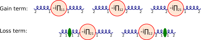
Figure 4: Grouping the diagrams for rescattering. Here, the green ovals represent the diagrams at $O(A^{\frac{2}{3}}g^{6})$ while the circles denote 2PI self-energies.

For the simplicity of the color and Lorentz indices, we shall calculate

$$\bar{G}_{22}(X,p)\equiv\frac{\sum_{\lambda}\epsilon_{\lambda\nu}(p)\epsilon^{*}_{\lambda\mu}(p)}{2(N_{c}^{2}-1)}\,G_{22}^{a\mu,a\nu}(X,p).$$ (68)

As illustrated in Fig. 4, we can group the subset of diagrams into a gain term and a loss term in the kinetic theory notation, with the circles denoting 2PI self-energies $\Pi_{ij}$. In the gain term two classical $G_{22}^{a\mu,b\mu}$ are used in the calculation of the self-energies, $\Pi$’s, while in the loss term only one classical $G_{22}^{a\mu,b\mu}$ is used in $\Pi$’s and the other classical correlator is placed on one of the external gluon propagators, as shown by the green ovals in Fig. 4.

In terms of the averaged self-energies

$$\bar{\Pi}\equiv\frac{\sum_{\lambda}\epsilon_{\lambda\nu}(p)\epsilon^{*}_{\lambda\mu}(p)\Pi^{a\mu,b\nu}(X,p)}{2(N_{c}^{2}-1)},$$ (69)

the gain term takes the form

$$\bar{G}_{22}^{gain}(X,p)= -i\int d^{4}x\,e^{ip\cdot x}\int d^{4}z\,e^{-ip^{\prime}\cdot z}\int\frac{d^{4}Z\,d^{4}p^{\prime}}{(2\pi)^{4}}$$

$$\times\left[G^{(0)}_{21}\left(X-Z+\frac{x-z}{2}\right)\bar{\Pi}_{11}\left(Z,p^{\prime}\right)G^{(0)}_{12}\left(Z-X+\frac{x-z}{2}\right)\right.$$

$$\left.+G^{(0)}_{21}\left(X-Z+\frac{x-z}{2}\right)\bar{\Pi}_{12}\left(Z,p^{\prime}\right)G^{(0)}_{22}\left(Z-X+\frac{x-z}{2}\right)\right.$$

$$\left.+G^{(0)}_{22}\left(X-Z+\frac{x-z}{2}\right)\bar{\Pi}_{21}\left(Z,p^{\prime}\right)G^{(0)}_{12}\left(Z-X+\frac{x-z}{2}\right)\right].$$ (70)

To evaluate this expression we write the retarded Green function $G^{(0)}_{21}(x)$ in the form of (48), while the advanced and cut Green functions are

$$G^{(0)}_{12}(x)=G_{A}(x)=-\theta(-x^{+})\,\theta(-x^{-})\int\frac{d^{2}k_{\perp}\,dk^{+}}{(2\pi)^{3}\,2k^{+}}\,e^{-ik\cdot x}\qquad\text{with $k^{-}=\frac{\underline{k}^{2}}{2k^{+}}$}$$ (71)

and

$$G^{(0)}_{22}(x)=\int\frac{d^{4}k}{(2\pi)^{4}}\,e^{-ik\cdot x}\,\pi\,\delta(k^{2})=\frac{1}{2}\int\frac{d^{2}k_{\perp}\,dk^{+}}{(2\pi)^{3}\,2|k^{+}|}\,e^{-ik\cdot x}.$$ (72)

Integrating over $z$, $p^{\prime}$, $\underline{x}$ we arrive at

$$\bar{G}_{22}^{gain}(X,p)=i\int\frac{d^{2}k_{\perp}\,dk^{+}}{(2\pi)^{3}\,2k^{+}}\frac{4\,dk^{\prime\,+}}{4\pi k^{\prime\,+}}\,e^{-i(k-k^{\prime})\cdot(X-Z)}\,d^{4}Z$$ (73)

$$\times\,\left\{\theta(X^{+}-Z^{+})\theta(X^{-}-Z^{-})\int\limits_{-2(X^{+}-Z^{+})}^{2(X^{+}-Z^{+})}dy^{+}e^{i\,\left(p^{-}-\frac{k^{-}+k^{\prime\,-}}{2}\right)y^{+}}\right.$$

$$\hskip 85.35826pt\times\,\int\limits_{-2(X^{-}-Z^{-})}^{2(X^{-}-Z^{-})}dy^{-}e^{i\,\left(p^{+}-\frac{k^{+}+k^{\prime\,+}}{2}\right)y^{-}}\,\bar{\Pi}_{11}(Z,P)$$

$$-\frac{\mbox{Sign}(k^{\prime\,+})}{2}\,\int\limits_{-2(X^{+}-Z^{+})}^{\infty}dy^{+}e^{i\,\left(p^{-}-\frac{k^{-}+k^{\prime\,-}}{2}\right)y^{+}}\int\limits_{-2(X^{-}-Z^{-})}^{\infty}dy^{-}e^{i\,\left(p^{+}-\frac{k^{+}+k^{\prime\,+}}{2}\right)y^{-}}\,\bar{\Pi}_{12}(Z,P)$$

$$\left.+\frac{\mbox{Sign}(k^{+})}{2}\,\int\limits_{-\infty}^{2(X^{+}-Z^{+})}dy^{+}e^{i\,\left(p^{-}-\frac{k^{-}+k^{\prime\,-}}{2}\right)y^{+}}\int\limits_{-\infty}^{2(X^{-}-Z^{-})}dy^{-}e^{i\,\left(p^{+}-\frac{k^{+}+k^{\prime\,+}}{2}\right)y^{-}}\,\bar{\Pi}_{21}(Z,P)\right\}$$

where we have defined $y^{\pm}=x^{\pm}-z^{\pm}$. Here $\underline{k}^{\prime}=2\underline{p}-\underline{k}$.

To reproduce kinetic theory one has to assume that gluons go on mass shell between interactions. This means the time between rescatterings is long enough for the gluons to go on mass shell. Therefore, we need to assume that $X^{+}-Z^{+}$ and $X^{-}-Z^{-}$ are very large in Eq. (73). This approximation is different from simply assuming that $X^{+}$ and $X^{-}$ are large, as was done in Eqs. (51), since the integrals over $Z^{+}$ and $Z^{-}$ in Eq. (73) are not restricted to the regions far away from $X^{+}$ and $X^{-}$ respectively. Thus we simply assume that the large-$X^{+}-Z^{+}$ and $X^{-}-Z^{-}$ region dominates in the integral. This assumption is needed to obtain kinetic theory from our formalism, but cannot be easily justified otherwise for the collision at hand.

When assuming that a dimensionful quantity is large one has to compare it to another dimensionful quantity. Unfortunately this is hard in our case, since almost everything else is integrated out. We simply state that $X^{+}-Z^{+}$ and $X^{-}-Z^{-}$ are the largest distance scales in the problem, with the possible exception of $Z^{+}$ and $Z^{-}$ which may be comparable. Note that in deriving the classical correlator (65) we have assumed that $X^{+}$ and $X^{-}$ are large (see (51)): in the problem at hand, $X^{+}$ and $X^{-}$ from Eq. (66) become $Z^{+}$ and $Z^{-}$ since we will be using the classical correlators to calculate $\bar{\Pi}_{ij}$. Therefore, our $Z^{+}$ and $Z^{-}$ have already been assumed to be very large.

Finally, a question remains whether to send $X^{+}-Z^{+}$ and $X^{-}-Z^{-}$ to $+\infty$ or to $-\infty$ when taking them large: from the curly brackets in Eq. (73) we see that only the $X^{+}-Z^{+}\to+\infty$ and $X^{-}-Z^{-}\to+\infty$ limits give a non-zero result. Applying those limits to Eq. (73) with the help of Eqs. (51) and integrating out $k^{+}$, $k^{\prime\,+}$ and $\underline{Z}$ afterwards while assuming that $\bar{\Pi}_{ij}(Z^{+},Z^{-},\underline{Z},P)=\bar{\Pi}_{ij}(Z^{+},Z^{-},P)$ due to the slowly changing transverse profile of the large nucleus yields

$$\bar{G}_{22}^{gain}(X,p)=i\int\limits_{0}^{X^{+}}dZ^{+}\int\limits_{0}^{X^{-}}dZ^{-}\,\frac{\cos(c_{X-Z}\sqrt{p^{2}})}{\sqrt{2p^{+}p^{-}p^{2}}}\left[\bar{\Pi}_{11}+\frac{\mbox{Sign}(p^{+})}{2}(\bar{\Pi}_{21}-\bar{\Pi}_{12})\right],$$ (74)

where

$$c_{X-Z}=2\tau_{X-Z}\sinh(y-\eta_{X-Z})$$ (75)

with

$$\tau_{X-Z}\equiv\sqrt{2(X^{+}-Z^{+})(X^{-}-Z^{-})},\qquad\eta_{X-Z}\equiv\frac{1}{2}\ln\left(\frac{X^{+}-Z^{+}}{X^{-}-Z^{-}}\right).$$ (76)

In arriving at Eq. (74) we put $p^{2}=0$ in the argument of the Sign-function: this approximation will be justified shortly. Lower limits of the $Z^{+}$ and $Z^{-}$ integrals were set to zero in Eq. (74) due to the classical correlator (66) which we will use to calculate $\bar{\Pi}_{ij}$: the correlator ensures that no gluons are produced before the heavy ion collision at $(t,z)=(0,0)$.

It is important to point out that, even though we assumed that $X^{+}-Z^{+}$ and $X^{-}-Z^{-}$ are very large, we have set the upper limits of the $Z^{+}$ and $Z^{-}$ integrations in Eq. (74) to $X^{+}$ and $X^{-}$ respectively. This is related to the fact that our calculation requires that $X^{+}-Z^{+}$ and $X^{-}-Z^{-}$ are large, but does not tell us whether they need to be larger than $Z^{+}$ and $Z^{-}$. For instance, large $X^{+}-Z^{+}$ may imply either of the following situations (ditto for $X^{-}-Z^{-}$):

• $X^{+}-Z^{+}\gg 1/Q_{s}$, $Z^{+}\gg 1/Q_{s}$; or

• $X^{+}-Z^{+}\gg Z^{+}\gg 1/Q_{s}$.

As we will see below, the two limits give different results. As we mentioned in the Introduction, we will answer the question of whether regime (i) or (ii) is correct by a more detailed calculation in our next paper KovchegovWu .

By assuming that $\tau_{X-Z}$ is sufficiently large once again and using (63), we obtain

$$\bar{G}_{22}^{gain}(X,p)= \frac{i\pi}{p_{\perp}}\,\delta(p^{2})\,\int\limits_{0}^{X^{+}}dZ^{+}\int\limits_{0}^{X^{-}}dZ^{-}\,\delta(y-\eta_{X-Z})\,\frac{1}{\tau_{X-Z}}$$

$$\times\left[\bar{\Pi}_{11}(Z,p)+\frac{\mbox{Sign}(p^{0})}{2}\left(\bar{\Pi}_{21}(Z,p)-\bar{\Pi}_{12}(Z,p)\right)\right].$$ (77)

Now let us turn our attention to the loss term. We will make similar approximations while evaluating the loss term in Fig. 4. The exact starting form of the loss term is as follows

$$\bar{G}^{loss}_{22}(X,p)= -i\int d^{4}xe^{ip\cdot x}\int d^{4}z_{1}d^{4}z_{2}$$

$$\times\left[G^{(0)}_{21}\left(X+\frac{x}{2}-z_{1}\right)\,\bar{\Pi}_{12}(z_{1},z_{2})\,\bar{G}^{cl}_{22}\left(z_{2},X-\frac{x}{2}\right)\right.$$

$$\left.+\bar{G}^{cl}_{22}\left(X+\frac{x}{2},z_{1}\right)\bar{\Pi}_{21}(z_{1},z_{2})\,G^{(0)}_{12}\left(z_{2}-X+\frac{x}{2}\right)\right],$$ (78)

where $\bar{G}^{cl}_{22}$ is obtained by substituting the classical correlator $G_{22}^{a\mu,b\nu}$ from (65) into (68). Similar to the above we define $Z=(z_{1}+z_{2})/2$, $z=z_{1}-z_{2}$ and write

$$\bar{G}^{loss}_{22}(X,p)= -i\int d^{4}xe^{ip\cdot x}\int d^{4}Zd^{4}z\frac{d^{4}p^{\prime}}{(2\pi)^{4}}\,e^{-ip^{\prime}\cdot z}\,$$

$$\times\left[G^{(0)}_{21}\left(X-Z+\frac{x-z}{2}\right)\,\bar{\Pi}_{12}(Z,p^{\prime})\,\bar{G}^{cl}_{22}\left(Z-\frac{z}{2},X-\frac{x}{2}\right)\right.$$

$$\left.+\,\bar{G}^{cl}_{22}\left(X+\frac{x}{2},Z+\frac{z}{2}\right)\bar{\Pi}_{21}(Z,p^{\prime})\,G^{(0)}_{12}\left(Z-X+\frac{x-z}{2}\right)\right]$$ (79)

with

$$\bar{\Pi}_{ij}(z_{1},z_{2})=\bar{\Pi}_{ij}\left(Z+\frac{z}{2},Z-\frac{z}{2}\right)=\int\frac{d^{4}p^{\prime}}{(2\pi)^{4}}\,e^{-ip^{\prime}\cdot z}\,\bar{\Pi}_{ij}(Z,p^{\prime}).$$ (80)

Integrating over $z$, $p^{\prime}$ and $\underline{x}$ yields

$$\bar{G}^{loss}_{22}(X,p)=i\int\frac{d^{2}k_{\perp}\,dk^{+}}{(2\pi)^{3}\,2k^{+}}\frac{4\,dk^{\prime\,+}}{4\pi k^{\prime\,+}}\,e^{i(k-k^{\prime})\cdot(X-Z)}\,d^{4}Z\,f^{cl}\left(\frac{X+Z}{2},k^{\prime}\right)$$ (81)

$$\times\,\left\{\mbox{Sign}(k^{\prime\,+})\,\int\limits_{-\infty}^{2(X^{+}-Z^{+})}dy^{+}e^{i\,\left(p^{-}-\frac{k^{-}+k^{\prime\,-}}{2}\right)y^{+}}\int\limits_{-\infty}^{2(X^{-}-Z^{-})}dy^{-}e^{i\,\left(p^{+}-\frac{k^{+}+k^{\prime\,+}}{2}\right)y^{-}}\,\bar{\Pi}_{21}(Z,P)\right.$$

$$\left.-\mbox{Sign}(k^{+})\,\int\limits_{-2(X^{+}-Z^{+})}^{\infty}dy^{+}e^{i\,\left(p^{-}-\frac{k^{-}+k^{\prime\,-}}{2}\right)y^{+}}\int\limits_{-2(X^{-}-Z^{-})}^{\infty}dy^{-}e^{i\,\left(p^{+}-\frac{k^{+}+k^{\prime\,+}}{2}\right)y^{-}}\,\bar{\Pi}_{12}(Z,P)\right\}$$

where again $y^{\pm}=x^{\pm}-z^{\pm}$ along with $\underline{k}^{\prime}=2\underline{p}-\underline{k}$. We have also assumed that $x^{\pm}$ and $z^{\pm}$ are much smaller than $X^{\pm}$ and $Z^{\pm}$ and neglected $x^{\pm}$ and $z^{\pm}$ in the argument of $f^{cl}$.

Assuming that $X^{+}-Z^{+}\to+\infty$ and $X^{-}-Z^{-}\to+\infty$ and $\bar{\Pi}_{ij}(Z^{+},Z^{-},\underline{Z},P)=\bar{\Pi}_{ij}(Z^{+},Z^{-},P)$ we integrate over $y^{+}$, $y^{-}$, $\underline{Z}$, $k^{+}$ and $k^{\prime\,+}$ obtaining

$$\bar{G}^{loss}_{22}(X,p)=i\int\limits_{0}^{X^{+}}dZ^{+}\int\limits_{0}^{X^{-}}dZ^{-}\,\frac{\cos(c_{X-Z}\sqrt{p^{2}})}{\sqrt{2p^{+}p^{-}p^{2}}}\,\mbox{Sign}(p^{+})\,(\bar{\Pi}_{21}-\bar{\Pi}_{12})\,f^{cl}\left(\frac{X+Z}{2},p\right)$$ (82)

where again we have put $p^{2}=0$ in the argument of the Sign-function along with the argument of $f^{cl}$.

Finally, invoking the late-time argument again we apply Eq. (63) to Eq. (82). This gives

$$\bar{G}_{22}^{loss}(X,p)= \,\frac{i\pi}{p_{\perp}}\,\delta(p^{2})\int_{0}^{X^{+}}dZ^{+}\int_{0}^{X^{-}}dZ^{-}\,\delta(y-\eta_{X-Z})\frac{1}{\tau_{X-Z}}$$

$$\times\mbox{Sign}(p^{0})\,\left[\bar{\Pi}_{21}(Z,p)-\bar{\Pi}_{12}(Z,p)\right]f^{cl}\left(\frac{X+Z}{2},p\right).$$ (83)

4.2 Gluon self-energies

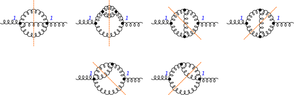
Figure 5: Diagrams for $\Pi_{11}^{a\mu,b\nu}$. In each diagram the dashed orange line cuts through all the $2-2$ propagators, separating the diagram into a product of an amplitude and a complex conjugate amplitude.

We first evaluate the gluon self energy $\Pi_{11}^{a\mu,b\nu}$ from the diagrams in Fig. 5. Without loss of generality (for the late-time approximation at hand), we assume that the gluon propagators in these diagrams take the following form

$$G_{22}^{a\mu,b\nu}(X,p)=2\pi\delta(p^{2})\delta^{ab}\sum_{\lambda}\epsilon_{\lambda}^{\mu}(p)\epsilon_{\lambda}^{*\nu}(p)\,g_{22}(X,p),$$

$$G_{21}^{a\mu,b\nu}(X,p)=G_{R}^{a\mu,b\nu}(p),\qquad G_{12}^{a\mu,b\nu}(X,p)=G_{A}^{a\mu,b\nu}(p),$$ (84)

with $g_{22}(X,p)=1/2$ for the free one and $g_{22}(X,p)=f^{cl}(X,p)$ for the classical one. For our problem, we need only to include vertices with only one “1” field. In each diagram there are three $2-2$ propagators according to the counting rule in (139).

In our calculation, we choose to label by $p_{1},p_{2},p_{3}$ the momenta of the three $2-2$ propagators in each diagram. These will be our integration variables. They satisfy $p=p_{1}+p_{2}+p_{3}$. Each propagator has a positive- and negative-frequency part. We shall take the external momentum $p^{+}$ to be positive, and, in view of the above calculation of the gain and loss term, on mass shell, $p^{2}=0$. In each diagram, while evaluating loop integrals, there should be only two lines out of $p_{1},p_{2},p_{3}$-carrying 2-2 lines with the positive-frequency parts of the propagators, while the remaining third line would come in with the negative-frequency part. It is clear that the diagrams in Fig. 5 reduce to the $gg\to gg$ scattering amplitude squared. Except for the first diagram in Fig. 5, different choices of positive- and negative-frequency parts for the 2-2 lines give us the products of $s-$, $t-$ and $u-$ channel amplitudes and their conjugates. Since $p_{1},p_{2}$ and $p_{3}$ are dummy variables to be integrated out, we redefine $p_{1}$ as the negative-frequency momentum and replace $p_{1}\to-p_{1}$ such that the new $p_{1}$ would have a positive frequency. Then, by collecting all terms obtained in this way, we arrive at the following result

$$-i\bar{\Pi}_{11} =-\frac{1}{2}\int_{p_{1},p_{2},p_{3}}(2\pi)^{4}\delta(p+p_{1}-p_{2}-p_{3})$$

$$\times\,\overline{|M|^{2}}\,g_{22}(X,p_{1})\,g_{22}(X,p_{2})\,g_{22}(X,p_{3}),$$ (85)

where

$$\overline{|M|^{2}}=8N_{c}^{2}g_{s}^{4}\left(3-\frac{tu}{s^{2}}-\frac{su}{t^{2}}-\frac{st}{u^{2}}\right),$$ (86)

and for brevity we have denoted

$$\int_{p}\equiv\int\frac{d^{3}p}{(2\pi)^{3}2\omega_{p}},$$ (87)

with $\omega_{p}=|{\vec{p}}|$ and the Mandelstam variables defined by

$$s=(p+p_{1})^{2},\qquad t=(p-p_{2})^{2},\qquad u=(p-p_{3})^{2}.$$ (88)

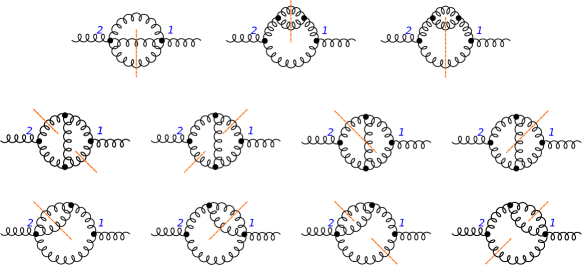
Figure 6: Diagrams for $-i\Pi_{21}^{a\mu,b\nu}$. In each diagram the dashed orange line cuts through two $2-2$ propagators.

Next, let us calculate $-i[\bar{\Pi}_{21}-\bar{\Pi}_{12}]$, which are given by 2 times the real parts of the diagrams in Fig. 6. As indicated by the dashed lines in this figure, there are only two $2-2$ propagators in each diagram. Compared to each corresponding diagram for $\bar{\Pi}_{11}$ in Fig. 5, the diagrams in Fig. 6 have a retarded (or advanced) propagator instead of the third $2-2$ propagator. Then, by subtracting out $\bar{\Pi}_{12}$ from $\bar{\Pi}_{21}$ one converts the retarded (advanced) propagator into a on-mass shell $\delta$-function with different signs for its positive- and negative-frequency parts. After this, using the same trick as that for $\Pi_{11}$ with the positive and negative energy parts of the propagators, we get

$$-i [\bar{\Pi}_{21}(X,p)-\bar{\Pi}_{12}(X,p)]=\frac{1}{2}\int_{p_{1},p_{2},p_{3}}(2\pi)^{4}\delta(p+p_{1}-p_{2}-p_{3})\,\overline{|M|^{2}}$$

$$\times\,\left[g_{22}(X,p_{1})\,g_{22}(X,p_{2})+g_{22}(X,p_{1})\,g_{22}(X,p_{3})-g_{22}(X,p_{2})\,g_{22}(X,p_{3})\right].$$ (89)

4.3 Comparison with kinetic theory

In this subsection we evaluate $\bar{G}_{22}(X,p)$ using the self-energies calculated in the previous subsection. Since both the gain (77) and loss (83) terms are proportional to $\delta(p^{2})$, quasi-particle picture applies; therefore, as a comparison we also calculate the distribution function at $O(\alpha_{s}^{2})$ by performing a perturbative solution of the Boltzmann equation.

4.3.1 Results from the above approximation

Inserting (85) and (89) into (77) and (83) gives

$$\bar{G}_{22}^{gain}(X,p)= \int_{0}^{X^{+}}dZ^{+}\int_{0}^{X^{-}}dZ^{-}\frac{\pi}{p_{\perp}\tau_{X-Z}}\delta(p^{2})\delta(y-\eta_{X-Z})$$

$$\times\frac{1}{2}\int_{p_{1},p_{2},p_{3}}(2\pi)^{4}\delta(p+p_{1}-p_{2}-p_{3})\overline{|M|^{2}}f^{cl}(Z,p_{2})f^{cl}(Z,p_{3}),$$ (90)

$$\bar{G}_{22}^{loss}(X,p)= -\int_{0}^{X^{+}}dZ^{+}\int_{0}^{X^{-}}dZ^{-}\frac{\pi}{p_{\perp}\tau_{X-Z}}\delta(p^{2})\delta(y-\eta_{X-Z})$$

$$\times\frac{1}{2}\int_{p_{1},p_{2},p_{3}}(2\pi)^{4}\delta(p+p_{1}-p_{2}-p_{3})f^{cl}(Z,p_{1})f^{cl}\left(\frac{X+Z}{2},p\right).$$ (91)

Both terms give a boost-invariant (rapidity-independent) particle distribution. This is more transparent if one uses the following variables

$$\tau_{Z}=\sqrt{2Z^{+}Z^{-}},\qquad\eta_{Z}=\frac{1}{2}\ln\frac{Z^{+}}{Z^{-}}.$$ (92)

Since our approximation should break down at early times, we require $\tau_{Z}>\tau_{0}$ with $\tau_{0}$ some initial time. Since $f^{cl}(X,p)\propto\delta(\eta-y)$, it is convenient to take

$$\int_{p_{i}}=\int\frac{d^{4}p_{i}}{(2\pi)^{4}}\theta(p_{i}^{0})2\pi\delta(p_{i}^{2})=\frac{1}{2}\int\frac{dy_{i}\,d^{2}p_{i}}{(2\pi)^{3}}.$$ (93)

Let us start with the gain term. Using Eq. (66) we write

$$\bar{G}_{22}^{gain}(X,p)=\frac{\delta(p^{2})}{16p_{\perp}}\prod\limits_{i=1}^{3}\int\frac{d^{2}p_{i}}{(2\pi)^{2}}(2\pi)^{2}\delta(\underline{p}+\underline{p}_{1}-\underline{p}_{2}-\underline{p}_{3})$$

$$\qquad\times f_{\perp}^{cl}(p_{2\perp})f_{\perp}^{cl}(p_{3\perp})\int\limits_{\tau_{0}}^{\tau}\frac{d\tau_{Z}}{\tau_{Z}}\int\limits_{-\ln\frac{\tau}{\tau_{Z}}+\eta}^{\ln\frac{\tau}{\tau_{Z}}+\eta}d\eta_{Z}\frac{1}{\tau_{X-Z}}\delta(y-\eta_{X-Z})\,\overline{|M|^{2}}$$

$$\qquad\times\int dy_{1}\delta(p_{\perp}e^{y}+p_{1\perp}e^{y_{1}}-p_{23\perp}e^{\eta_{Z}})\delta(p_{\perp}e^{-y}+p_{1\perp}e^{-y_{1}}-p_{23\perp}e^{-\eta_{Z}})$$ (94)

with $p_{23\perp}\equiv p_{2\perp}+p_{3\perp}$. By integrating out $y_{1}$ and $\eta_{Z}$ we have

$$\bar{G}_{22}^{gain}(X,p)=\frac{\delta(p^{2})}{16p_{\perp}}\prod\limits_{i=1}^{3}\int\frac{d^{2}{p}_{i}}{(2\pi)^{2}}(2\pi)^{2}\delta(\underline{p}+\underline{p}_{1}-\underline{p}_{2}-\underline{p}_{3})\frac{f_{\perp}^{cl}(p_{\perp 2})f_{\perp}^{cl}(p_{\perp 3})}{\mathcal{P}^{2}(p_{\perp},p_{1\perp},p_{2\perp},p_{3\perp})}$$

$$\times\sum_{\{\eta_{Z},y_{1}\}}\int_{\tau_{0}}^{\tau}\frac{d\tau_{Z}}{\tau_{Z}}\frac{1}{\tau_{X-Z}}\delta(y-\eta_{X-Z})\,\overline{|M|^{2}}\,\theta\left(e^{\eta-\eta_{Z}}-\frac{\tau_{Z}}{\tau}\right)\theta\left(e^{\eta_{Z}-\eta}-\frac{\tau_{Z}}{\tau}\right),$$ (95)

where

$$\mathcal{P}^{2}(p_{\perp},p_{1\perp},p_{2\perp},p_{3\perp})\equiv\sqrt{[(p_{1\bot}-p_{\bot})^{2}-p_{23\bot}^{2}][(p_{1\bot}+p_{\bot})^{2}-p_{23\bot}^{2}]}$$ (96)

and the sum over $\{y_{1},\eta_{Z}\}$ goes over the following two values for each variable

$$e^{y_{1}-y}=\frac{\pm\mathcal{P}^{2}\left(p_{\bot},p_{1\bot},p_{2\bot},p_{3\bot}\right)-p_{1\bot}^{2}+p_{23\bot}^{2}-p_{\bot}^{2}}{2p_{1\bot}p_{\bot}},$$

$$e^{\eta_{Z}-y}=\frac{\pm\mathcal{P}^{2}\left(p_{\bot},p_{1\bot},p_{2\bot},p_{3\bot}\right)-p_{1\bot}^{2}+p_{23\bot}^{2}+p_{\bot}^{2}}{2\,p_{23\bot}\,p_{\bot}}.$$ (97)

The above two solutions for $\{y_{1},\eta_{Z}\}$ respectively give

$$\sinh(y-\eta_{Z})=\pm\frac{\mathcal{P}^{2}(p_{\perp},p_{1\perp},p_{2\perp},p_{3\perp})}{2\,p_{23\perp}\,p_{\perp}}\equiv\pm\frac{\hat{p}_{z}}{p_{\perp}}.$$ (98)

Now let us integrate out $\tau_{Z}$. The $\delta$-function in Eq. (95) gives

$$\tau_{Z}=\frac{\sinh(y-\eta)}{\sinh(y-\eta_{Z})}\tau,\qquad\tau_{X-Z}=\frac{\sinh(\eta-\eta_{Z})}{\sinh(y-\eta_{Z})}\tau,$$ (99)

and the Jacobian

$$J\equiv\frac{1}{\left|\frac{d}{d\tau_{Z}}(y-\eta_{X-Z})\right|}=\frac{\tau_{Z}\,\tau_{X-Z}}{\tau|\sinh(y-\eta)|}.$$ (100)

From the above equations, we finally obtain

$$\bar{G}_{22}^{gain}(X,p) =\frac{\delta(p^{2})}{16p_{\perp}\,\tau}\prod\limits_{i=1}^{3}\int\frac{d^{2}\underline{p}_{i}}{(2\pi)^{2}}(2\pi)^{2}\delta(\underline{p}+\underline{p}_{1}-\underline{p}_{2}-\underline{p}_{3})\frac{f_{\perp}^{cl}(p_{\perp 2})f_{\perp}^{cl}(p_{\perp 3})}{\mathcal{P}^{2}(p_{\perp},p_{1\perp},p_{2\perp},p_{3\perp})}$$

$$\times\frac{\overline{|M|^{2}}}{|\sinh(y-\eta)|}\theta\left(p_{\perp}|\sinh(y-\eta)|-\hat{p}_{z}\tau_{0}/\tau\right)\theta\left(\hat{p}_{z}-p_{\perp}|\sinh(y-\eta)|\right)$$

$$\times\theta\left(e^{\eta-\eta_{Z}}-\frac{p_{\perp}|\sinh(y-\eta)|}{\hat{p}_{z}}\right)\theta\left(e^{\eta_{Z}-\eta}-\frac{p_{\perp}|\sinh(y-\eta)|}{\hat{p}_{z}}\right),$$ (101)

where $\eta-\eta_{Z}$ should have the same sign as $y-\eta_{Z}$ and $y-\eta$, and $\{y_{1},\eta_{Z}\}$ only assume the values in (97) which ensure that $\tau_{Z}$ is positive.

For the loss term (91) evaluation appears to be more complicated in general. The difficulty is in the $(X+Z)/2$ in the argument of one of the $f^{cl}$ in (91). It appears that to obtain something similar to kinetic theory one has to replace

$$\frac{X+Z}{2}\to Z$$ (102)

in the argument of $f^{cl}$ in (91). This is an ad hoc assumption, particularly for the plus and minus components $X^{\pm},Z^{\pm}$, which does not follow from the orderings (i) and (ii) considered above. In fact, it can never be realized in the case of ordering (ii). Within ordering (i) one could imagine a situation where

$$Z^{+}\gg X^{+}-Z^{+}\gg 1/Q_{s}$$ (103)

and the replacement (102) may be justified. Such a condition is a further refinement of the ordering (ii) and was not needed for the gain term. Below we will assume that the ordering (103) applies and make the substitution (102).

Working in this approximation one can easily integrate out $\eta_{Z}$ and $y_{1}$ in Eq. (91) and get

$$\bar{G}_{22}^{loss}(X,p)=-\frac{\delta(p^{2})}{16p_{\perp}}\prod\limits_{i=1}^{3}\int\frac{d^{2}\underline{p}_{i}}{(2\pi)^{2}}(2\pi)^{2}\delta(\underline{p}+\underline{p}_{1}-\underline{p}_{2}-\underline{p}_{3})$$

$$\qquad\times f_{\perp}^{cl}(p_{\perp})f_{\perp}^{cl}(p_{1\perp})\int_{\tau_{0}}^{\tau}\frac{d\tau_{Z}}{\tau_{Z}}\frac{1}{\tau_{X-Z}}\delta(y-\eta_{X-Z})\overline{|M|^{2}}$$

$$\qquad\times\int dy_{2}dy_{3}\delta((p_{\perp}+p_{1\perp})e^{y}-p_{2\perp}e^{y_{2}}-p_{3\perp}e^{y_{3}})$$

$$\times\delta((p_{\perp}+p_{1\perp})e^{-y}-p_{2\perp}e^{-y_{2}}-p_{3\perp}e^{-y_{3}})\theta\left(e^{\eta-y}-\frac{\tau_{Z}}{\tau}\right)\theta\left(e^{y-\eta}-\frac{\tau_{Z}}{\tau}\right)$$ (104)

with $\eta_{Z}=y$. Now we are left with

$$\delta(y-\eta_{X-Z})=\frac{\tau-\tau_{Z}}{\tau}\delta(y-\eta).$$ (105)

At the end, we have

$$\bar{G}_{22}^{loss}(X,p)=-\frac{\delta(p^{2})}{16p_{\perp}\tau}\ln\left(\frac{\tau}{\tau_{0}}\right)\prod\limits_{i=1}^{3}\int\frac{d^{2}\underline{p}_{i}}{(2\pi)^{2}}(2\pi)^{2}\delta(\underline{p}+\underline{p}_{1}-\underline{p}_{2}-\underline{p}_{3})$$

$$\qquad\times\delta(y-\eta)\frac{f_{\perp}^{cl}(p_{\perp})f_{\perp}^{cl}(p_{1\perp})}{\mathcal{P}^{2}(p_{2\perp},p_{3\perp},p_{\perp},p_{1\perp})}\sum\limits_{\{y_{2},y_{3}\}}\overline{|M|^{2}}$$ (106)

with $\{y_{2},y_{3}\}$ summed over two values each given by the solutions to the equations resulting from the last two $\delta$ functions in (104).

We are now going to compare the results (101) and (106) of this Subsection for the gain and loss terms with the predictions of kinetic theory.

4.3.2 Results from the Boltzmann equation

In the boost-invariant and dilute ($f\ll 1$) system, the Boltzmann equation (161) reduces to Mueller:1999pi

$$\left(\frac{\partial}{\partial t}-\frac{1}{t}p_{z}\frac{\partial}{\partial p_{z}}\right)f=C[f](t,p_{\perp},p_{z})$$

$$\qquad\qquad\equiv\frac{1}{4\omega_{p}}\int_{p_{1},p_{2},p_{3}}\overline{|M|^{2}}[f_{2}f_{3}-ff_{1}](2\pi)^{4}\delta(p+p_{1}-p_{2}-p_{3}).$$ (107)

While the system we consider is boost-invariant (rapidity independent), we will concentrate on central rapidity, $\eta=0$, throughout this Subsection. At $\eta=0$ one has $\tau=t$.

In order to see the connection to the calculation in our formalism, we write

$$f=\sum\limits_{n=0}^{\infty}f^{(n)}\qquad\text{with $f^{(n)}$ being of $O(\alpha_{s}^{2n})$}.$$ (108)

The terms $f^{(n)}$ are to be found from solving the Boltzmann equation order-by-order in the coupling $\alpha_{s}$. The initial condition (the value of $f$ before the collision term becomes important) is given by saturation dynamics (cf. Eq. (66)),

$$f^{(0)}(t,p)=\frac{1}{t}f_{\perp}(p_{\perp})\delta(y),$$ (109)

which satisfies the “free” Boltzmann equation

$$\left(\frac{\partial}{\partial t}-\frac{1}{t}p_{z}\frac{\partial}{\partial p_{z}}\right)f^{(0)}=0.$$ (110)

The higher orders in $\alpha_{s}$ can be calculated by iteration

$$f^{(n+1)}=\int_{t_{0}}^{t}dt_{1}\,C[f^{(n)}](t_{1},tp_{z}/t_{1})+C^{(n+1)}(tp_{z}/t_{0})$$ (111)

with $C^{(n+1)}$ the constant of integration at $O(\alpha_{s}^{2(n+1)})$ and $t_{0}$ some initial time when the Boltzmann dynamics starts to apply (e.g. $t_{0}\sim 1/Q_{s}$).

For comparison with the results of the previous Subsection we need only to evaluate terms proportional to $O(\alpha_{s}^{2})$. According to (111), we first evaluate

$$C[f^{(0)}](t,p_{\perp},p_{z})=\frac{1}{32\pi t^{2}}\prod\limits_{i=1}^{3}\int\frac{d^{2}\underline{p}_{i}}{(2\pi)^{2}}(2\pi)^{2}\delta(\underline{p}+\underline{p}_{1}-\underline{p}_{2}-\underline{p}_{3})$$

$$\times\left.\left[\frac{f_{\perp}(p_{2\perp})f_{\perp}(p_{3\perp})}{2\omega_{p}\omega_{p_{1}}}\,\overline{|M|^{2}}\,\delta(\omega+\omega_{1}-p_{2\perp}-p_{3\perp})\right.\right|_{p_{1z}=-p_{z},\,p_{2z}=p_{3z}=0}$$

$$\left.\left.-\delta(y)\,\frac{2\,f_{\perp}(p_{\perp})\,f_{\perp}(p_{1\perp})}{p_{\perp}\mathcal{P}^{2}(p_{2\perp},p_{3\perp},p_{\perp},p_{1\perp})}\,\overline{|M|^{2}}\right|_{p_{1z}=0,\,|p_{2z}|=|p_{3z}|=\frac{\mathcal{P}^{2}(p_{2\perp},p_{3\perp},p_{\perp},p_{1\perp})}{2(p_{\perp}+p_{1\perp})}}\right].$$ (112)

To satisfy the initial conditions at time $t=t_{0}$ we put the integration constant to zero, $C^{(1)}=0$. Substituting Eq. (112) into Eq. (111) and integrating yields

$$f^{(1)}=\frac{1}{32\pi t}\,\prod\limits_{i=1}^{3}\int\frac{d^{2}\underline{p}_{i}}{(2\pi)^{2}}\,(2\pi)^{2}\,\delta(\underline{p}+\underline{p}_{1}-\underline{p}_{2}-\underline{p}_{3})$$ (113)

$$\times\left.\left[\frac{f_{\perp}(p_{2\perp})f_{\perp}(p_{3\perp})}{|p_{z}|\mathcal{P}^{2}(p_{\perp},p_{1\perp},p_{2\perp},p_{3\perp})}\,\theta(|p_{z}|-\hat{p}_{z}t_{0}/t)\,\theta(\hat{p}_{z}-|p_{z}|)\,\overline{|M|^{2}}\right|_{p_{1z}=-p_{z},\,p_{2z}=p_{3z}=0}\right.$$

$$\left.\left.-\delta(y)\ln\left(\frac{t}{t_{0}}\right)\frac{2\,f_{\perp}(p_{\perp})f_{\perp}(p_{1\perp})}{p_{\perp}\mathcal{P}^{2}(p_{2\perp},p_{3\perp},p_{\perp},p_{1\perp})}\,\overline{|M|^{2}}\right|_{p_{1z}=0,\,|p_{2z}|=|p_{3z}|=\frac{\mathcal{P}^{2}(p_{2\perp},p_{3\perp},p_{\perp},p_{1\perp})}{2(p_{\perp}+p_{1\perp})}}\right].$$

We obtain a linear combination of $\sim 1/t$ and $\sim\delta(y)\,(1/t)\,\ln(t/t_{0})$ terms. This is exactly the same $t$ and $y$-dependence as that in the previous Subsection for the gain and loss terms respectively (if we apply $\eta=0$ to those results).

Knowing the distribution function $f$ one can calculate the energy-momentum tensor using

$$T^{\mu\nu}(x)=2\,\int\limits_{p}\,p^{\mu}\,p^{\nu}\,f(x,p).$$ (114)

Clearly, the initial conditions (109), or, equivalently, the classical gluon correlator (66) give $T^{\mu\nu}\sim 1/\tau$ for all the non-zero components of the energy-momentum tensor, along with the longitudinal pressure $P_{L}=T^{33}(\eta=0)=0$: this behavior corresponds to free streaming of gluons. Adding the correction $f^{(1)}$ from Eq. (113) we obtain

$$\epsilon=\epsilon^{(0)}+\epsilon^{(1)}=\frac{A^{(0)}+\alpha_{s}^{2}\,A^{(1)}}{\tau}-\frac{\alpha_{s}^{2}\,B^{(1)}}{\tau}\,\ln\frac{\tau}{\tau_{0}},$$ (115a)

$$P_{T}=P_{T}^{(0)}+P_{T}^{(1)}=\frac{A^{(0)}+\alpha_{s}^{2}\,A^{(1)}-\alpha_{s}^{2}\,B^{(1)}}{\tau}-\frac{\alpha_{s}^{2}\,B^{(1)}}{\tau}\,\ln\frac{\tau}{\tau_{0}},$$ (115b)

$$P_{L}=P_{L}^{(1)}=\frac{\alpha_{s}^{2}\,B^{(1)}}{\tau}.$$ (115c)

The exact values of the coefficients $A^{(0)},A^{(1)}$ and $B^{(1)}$ can be found by explicit integration: their exact values are not important to us, as long as $A^{(1)}$ and/or $B^{(1)}$ are not zero. The $\sim 1/\tau$ and $\sim(1/\tau)\,\ln(\tau/\tau_{0})$ terms that $A^{(1)}$ and $B^{(1)}$ multiply constitute a deviation from the $\sim 1/\tau$ free-streaming behavior of the classical gluon fields. We conclude that kinetic theory predicts a deviation from free streaming after including a single $2\to 2$ rescattering correction to the classical gluon correlator. This prediction appears to agree with the results of the approximate calculations carried out above, after certain approximations were made. We will verify this prediction in KovchegovWu .

5 Free Streaming

Here we show how the above calculation can lead to different results depending on how the large-$X^{+}-Z^{+}$, $X^{-}-Z^{-}$ is imposed. In particular, we demonstrate that ordering (ii) from above does not lead to kinetic theory, but rather to free streaming of the produced gluons.

5.1 Free streaming after rescattering

In the calculations of Sec. 4.3.1 the integrations over $\tau_{Z}$ extend all the way up to $\tau$, in an apparent violation of the large-$X^{+}-Z^{+}$, $X^{-}-Z^{-}$ assumption used in deriving Eqs. (90) and (91). To preserve the main results (101) and (106) of Sec. 4.3.1 while satisfying the large-$X^{+}-Z^{+}$, $X^{-}-Z^{-}$ condition one could impose the ordering (i) from Sec. 4.1 in the following way:

$$\mbox{(i)}\ \ \tau_{0}\ll\tau_{z}\ll\xi\,\tau\ll\tau$$ (116)

with a small parameter $\xi\ll 1$ (but not too small, such that $\xi\tau\gg\tau_{0}$ still). For instance, we may have $\xi=\alpha_{s}^{\lambda}$ with some positive power $\lambda>0$. Replacing $\tau\to\xi\tau$ in the integration limits of Eq. (94) would still lead to $\bar{G}_{22}^{gain}(X,p)\sim 1/\tau$, just like in Eq. (101). Similarly, replacing $\tau\to\xi\tau$ in the upper integration limit and in the theta-functions of Eq. (104) one still obtains $\bar{G}_{22}^{loss}(X,p)\sim(1/\tau)\ln(\tau/\tau_{0})\,\delta(y-\eta)$, just like in (106). While the prefactors may be modified by the $\tau\to\xi\tau$ substitution, the $\tau$ and $\eta$ dependence of the gain and loss terms would remain the same. Hence, Eq. (116) appears to provide a more proper way of imposing the condition (i) on the calculation in Sec. 4.3.1.

It appears natural that in addition to the ordering (116) one also considers

$$\mbox{(ii)}\ \ \tau_{0}\ll\tau_{z}\ll\zeta\,\tau_{0}\ll\tau$$ (117)

where $\zeta\gg 1$ is a large parameter. For $\tau_{0}=1/Q_{s}$ one may have $\zeta=1/\alpha_{s}^{\omega}$ with $\omega>0$ such that $\zeta\tau_{0}=1/(\alpha_{s}^{\omega}\,Q_{s})$. While $\zeta$ is large, it should not be too large, such that $\zeta\,\tau_{0}\ll\tau$ still. Eq. (117) is consistent with the condition (ii) from Sec. 4.1 and also provides a way to impose the large-$X^{+}-Z^{+}$, $X^{-}-Z^{-}$ condition.

Replacing the upper limit of the $\tau_{Z}$ integration in Eq. (95) by using $\tau\to\zeta\,\tau_{0}$ (along with the same replacement in the arguments of $\theta$-functions, which we discard below since after for small $\tau_{Z}$ they are automatically satisfied) one gets

$$\bar{G}_{22}^{gain}(X,p)\sim\int\limits_{\tau_{0}}^{\zeta\,\tau_{0}}\frac{d\tau_{Z}}{\tau_{Z}}\frac{1}{\tau_{X-Z}}\delta(y-\eta_{X-Z})\approx\int\limits_{\tau_{0}}^{\zeta\,\tau_{0}}\frac{d\tau_{Z}}{\tau_{Z}}\,\frac{1}{\tau}\delta(y-\eta)=\frac{1}{\tau}\delta(y-\eta)\,\ln\zeta.$$ (118)

We have employed $\tau_{z}\ll\zeta\,\tau_{0}\ll\tau$ condition in simplifying Eq. (118). (Strictly-speaking we have assumed a somewhat stronger condition $Z^{\pm}\ll\zeta\,Z_{0}^{\pm}\ll X^{\pm}$ consistent with the original ordering (ii) to approximate $\tau_{X-Z}\approx\tau$ and $\eta_{X-Z}\approx\eta$.) We see that with the ordering (ii), (117), the gain contribution to the correlation function still scales as $1/\tau$, but now it is multiplied by $\delta(y-\eta)$: the $\delta$-function leads to zero longitudinal pressure, making this $\bar{G}_{22}^{gain}(X,p)$ consistent with free streaming.

The loss term is treated similarly: performing the $\tau\to\zeta\,\tau_{0}$ replacement in Eq. (104) gives

$$\bar{G}_{22}^{loss}(X,p)\sim\int\limits_{\tau_{0}}^{\zeta\,\tau_{0}}\frac{d\tau_{Z}}{\tau_{Z}}\frac{1}{\tau_{X-Z}}\delta(y-\eta_{X-Z})\approx\int\limits_{\tau_{0}}^{\zeta\,\tau_{0}}\frac{d\tau_{Z}}{\tau_{Z}}\,\frac{1}{\tau}\delta(y-\eta)=\frac{1}{\tau}\delta(y-\eta)\,\ln\zeta$$ (119)

which is also consistent with free streaming.

We conclude that while the calculations of Sec. 4.3.1 appear to be consistent with kinetic theory if the ordering (i) is imposed via (116), the same calculations are consistent with free streaming if the ordering (ii) is imposed with the help of (117). Therefore, since at this level of calculational precision we can not say whether the ordering (i) or (ii) is correct, we can not tell whether our calculation supports kinetic theory or the free-streaming scenario advocated in Kovchegov:2005ss .

5.2 A general argument for free streaming

For completeness, let us briefly recap the free-streaming argument from Kovchegov:2005ss , but now for the correlation function $\bar{G}_{22}$ considered in this work. (In Kovchegov:2005ss the argument was applied to the energy-momentum tensor of the medium produced in heavy ion collisions.) In a general case, involving all the possible multiple interactions and rescatterings, one can still write the $\bar{G}_{22}$ correlation function as a sum of the three diagrams in the top row of Fig. 5, but now without requiring that $\Pi_{ij}$ include 2PI diagrams only. The circles now denote any (connected) diagram. The resulting expression is the same as in Eq. (70):

$$\bar{G}_{22}(k,k^{\prime})=-i(2\pi)^{2}\delta(\underline{k}+\underline{k}^{\prime}) \left[G_{R}(k){\bar{\Pi}}_{11}(k,k^{\prime})G_{R}(k^{\prime})+G_{R}(k){\bar{\Pi}}_{12}(k,k^{\prime})G_{12}^{(0)}(k^{\prime})\right.$$

$$\left.+G_{22}^{(0)}(k){\bar{\Pi}}_{21}(k,k^{\prime})G_{R}(k^{\prime})\right].$$ (120)

Since all ${\bar{\Pi}}_{ij}$ are Lorentz-invariant, they can only be functions of $k^{2}$, $k^{\prime\,2}$ and $k\cdot k^{\prime}$. The ${\bar{\Pi}}_{ij}$’s can also be functions of $p\cdot k\sim k^{-}$, $p^{\prime}\cdot k\sim k^{+}$, $p\cdot k^{\prime}\sim k^{\prime\,-}$, and $p^{\prime}\cdot k^{\prime}\sim k^{\prime\,+}$ with $p$ and $p^{\prime}$ the momenta of the nucleons in nucleus $A_{1}$ and $A_{2}$. In Kovchegov:2005ss a “dictionary” was established by going through a number of examples. According to this “dictionary” the Fourier transform of the correlation function into coordinate space,

$$\bar{G}_{22}(x_{1},x_{2})=\int\frac{d^{4}k}{(2\pi)^{4}}\frac{d^{4}k^{\prime}}{(2\pi)^{4}}\,e^{-ik\cdot x_{1}-ik^{\prime}\cdot x_{2}}\,\bar{G}_{22}(k,k^{\prime}),$$ (121)

converts (modulo some prefactors and an index shift of the Bessel function resulting from the transform)

$$k^{2},k\cdot k^{\prime},k^{\prime\,2}\, \longrightarrow\,\frac{2k_{T}}{\tau},$$ (122a)

$$k^{\pm}\, \longrightarrow\,\frac{k_{T}\,e^{\pm\eta}}{\sqrt{2}}$$ (122b)

with $\eta$ the space-time rapidity. According to Eq. (122a), the leading late-$\tau$ contribution comes from putting $k^{2}=k\cdot k^{\prime}=k^{\prime\,2}=0$ in the ${\bar{\Pi}}_{ij}$’s, with corrections to it being suppressed by powers of $1/\tau$.

Let us illustrate this using the ${\bar{\Pi}}_{11}$ term in Eq. (5.2). Putting $k^{2}=k\cdot k^{\prime}=k^{\prime 2}=0$ in ${\bar{\Pi}}_{11}$ and integrating that term in (5.2) over $k^{-}$ and $k^{\prime\,-}$ yields

$${\bar{G}}_{22}(x_{1},x_{2})=-i\,\theta(x_{1}^{+})\,\theta(x_{2}^{+})\,\int\frac{d^{2}k_{\perp}}{(2\pi)^{2}}e^{i{\underline{k}}\cdot({\underline{x}}_{1}-{\underline{x}}_{2})}\int\limits_{-\infty}^{\infty}\frac{dk^{+}}{4\pi(k^{+}+i\epsilon)}$$ (123)

$$\times\,\int\limits_{-\infty}^{\infty}\frac{dk^{\prime+}}{4\pi(k^{\prime+}+i\epsilon)}e^{-ik^{+}x_{1}^{-}-i\frac{k_{\perp}^{2}}{2(k^{+}+i\epsilon)}x_{1}^{+}-ik^{\prime+}x_{2}^{-}-i\frac{k_{\perp}^{2}}{2(k^{\prime+}+i\epsilon)}x_{2}^{+}}\,{\bar{\Pi}}_{11}(k,k^{\prime})\Bigg{|}_{k^{2}=k\cdot k^{\prime}=k^{\prime 2}=0,\,\underline{k}^{\prime}=-\underline{k}}.$$

In arriving at Eq. (123) we have also neglected the $k^{\pm},k^{\prime\pm}$ dependence in ${\bar{\Pi}}_{11}$: below we will briefly outline how this can be reinstated. Employing

$$\int\limits_{-\infty}^{\infty}\frac{dk^{+}}{4\pi(k^{+}+i\epsilon)}\,e^{-ik^{+}x^{-}-i\frac{k_{\perp}^{2}}{2(k^{+}+i\epsilon)}x^{+}}=-\frac{i}{2}\theta(x^{-})\,J_{0}(k_{\perp}\tau)$$ (124)

we obtain

$$\bar{G}_{22}(x_{1},x_{2})= \,\frac{i}{4}\theta(x_{1}^{+})\,\theta(x_{2}^{+})\,\theta(x_{1}^{-})\,\theta(x_{2}^{-})\,\int\frac{d^{2}k_{\perp}}{(2\pi)^{2}}e^{i{\underline{k}}\cdot({\underline{x}}_{1}-{\underline{x}}_{2})}$$

$$\times\,J_{0}(k_{\perp}\tau_{1})J_{0}(k_{\perp}\tau_{2})\,{\bar{\Pi}}_{11}(k,k^{\prime})\Bigg{|}_{k^{2}=k\cdot k^{\prime}=k^{\prime 2}=0,\,\underline{k}^{\prime}=-\underline{k}}.$$ (125)

Clearly,

$$\bar{G}_{22}(x_{1},x_{2})\Bigg{|}_{\tau_{1}=\tau_{2}=\tau\to\infty}\sim\frac{1}{\sqrt{\tau_{1}\,\tau_{2}}}\Bigg{|}_{\tau_{1}=\tau_{2}=\tau}=\frac{1}{\tau}.$$ (126)

Hence the leading contribution to the correlator is $\sim 1/\tau$, corresponding to free streaming, as the energy-momentum tensor that one would obtain from the correlator (126) would scale as $T^{\mu\nu}\sim 1/\tau$. If there exist terms proportional to, say, Bjorken hydrodynamics Bjorken:1982qr , which has $T^{\mu\nu}\sim 1/\tau^{4/3}$, they would be subleading compared to the free-streaming term of Eq. (126).

Including the $k^{\pm},k^{\prime\pm}$-dependent terms in the above calculation would only add space-time rapidity dependence in the correlation function owing to Eq. (122b), without changing the conclusion (126) about the late-time asymptotics. Finally, the argument applies analogously to the ${\bar{\Pi}}_{12}$ and ${\bar{\Pi}}_{21}$ terms in Eq. (5.2).

The remaining question is whether the leading asymptotics happens to have a zero coefficient, that is, what if

$${\bar{\Pi}}_{11}(k,k^{\prime})+\frac{1}{2}\left[{\bar{\Pi}}_{21}(k,k^{\prime})-{\bar{\Pi}}_{12}(k,k^{\prime})\right]\Bigg{|}_{k^{2}=k\cdot k^{\prime}=k^{\prime 2}=0,\,\underline{k}^{\prime}=-\underline{k}}\overset{?}{=}0\,?$$ (127)

In Kovchegov:2005ss it was shown that for the energy-momentum tensor this is not the case. The leading late-time contribution was shown to be proportional to the particle (gluon) production cross section. Specifically, the energy density was shown to be

$$\epsilon(\tau,\eta,\underline{b})\Bigg{|}_{\tau\to\infty}=\frac{1}{\tau}\int d^{2}k_{T}\,k_{T}\,\frac{dN}{d^{2}k_{T}\,d\eta\,d^{2}b_{\perp}}.$$ (128)

Hence the leading free-streaming term is non-zero as long as one can define the multiplicity of produced gluons $dN/d^{2}k_{T}\,d\eta\,d^{2}b_{\perp}$, that is as long as perturbation theory holds.

6 Conclusions and Outlook

In this paper, we adapted the Schwinger-Keldysh formalism to study heavy-ion collisions in a perturbative QCD approach. We calculated the gluon two-point correlation function $G_{22}^{a\mu,b\nu}$ at $O(g^{6}A^{\frac{2}{3}})$ in the lowest-order classical approximation of the MV model. We found that at large $\tau$ the (quasi-) particle picture emerges from the classical field calculation at this order in the sense that

$$G_{22}^{a\mu,b\nu}(X,p)\propto\frac{2\pi}{\tau}\delta^{ab}\sum\limits_{\lambda=\pm}\epsilon_{\lambda}^{\mu}(k_{1})\epsilon_{\lambda}^{*\nu}(-k_{2})\delta(p^{2})\delta(y-\eta).$$ (129)

Motivated by this observation, we evaluated a subset of diagrams at $O(g^{16}A^{\frac{4}{3}})$, which are beyond the classical field approximation, and corresponds to a $2\to 2$ rescattering of the classically produced gluons. Each of these diagram includes two sub-diagrams of $O(g^{6}A^{\frac{2}{3}})$, described by $G_{22}^{a\mu,b\nu}$ in (129) each. In our calculation the rescattering occurs at some space-time point $Z^{\mu}$ while the gluon distribution is measured at another point $X^{\mu}$. We made the following approximations:

1. $\tau_{Z}\equiv\sqrt{2Z^{+}Z^{-}}\gg 1/Q_{s}$
   Under this assumption, each sub-diagram took the form in (129).

2. $\tau_{X-Z}\equiv\sqrt{2(X^{+}-Z^{+})(X^{-}-Z^{-})}\gg 1/Q_{s}$
   Under this assumption, the gluons after the rescattering can be taken to be quasi-classical particles. That is, they travel along a classical trajectory $X^{3}-Z^{3}=(X^{0}-Z^{0})p^{3}/p^{0}$ with $p^{\mu}$ the four-momentum of the gluons.

Under the above approximations, which are equivalent to case (i) listed above (or, for the loss term, by additionally imposing $\tau_{Z}\gg\tau_{X-Z}$), we find the rescattering correction consistent with a power series in $\alpha_{s}$ solution of the Boltzmann equation.

However, one needs to make a more detailed calculation to justify our approximations above. In our approximations of Eqs. (94) and (104) we put the upper limit of $\tau_{Z}$ integration to be $\tau$ in apparent violation of the assumption 2. We also do not know a priori whether our assumption 2 correctly represents the full diagrammatic calculation, since one may take another limit instead, $\tau\gg\tau_{Z}$, corresponding to case (ii) by the above counting. In this case $\bar{G}_{22}^{gain}$ and $\bar{G}_{22}^{loss}$ are still respectively given by (94) and (104) with another upper limit for $\tau_{Z}$ integration, as detailed in Sec. 5. If one takes the limit $\tau\to\infty$ in this case, both the gain and loss terms are proportional to $\delta(y-\eta)/\tau$. That is, after the rescattering the gluons assume a distribution similar to that for free-streaming particles. In the companion paper KovchegovWu we perform a detailed calculation in the framework of the $\lambda\varphi^{4}$ theory to explicitly identify which approximation is correct.

Appendix A The classical field limit

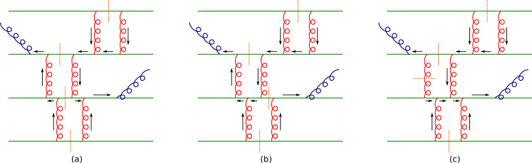
Figure 7: Illustration of diagrams in the classical limit. Diagrams (a) and (b) are separated into a product of two sub-diagrams connected to each other by $S^{(0)}_{22}$ cut quark propagators. Each of the sub-diagrams contributes to the classical field. In contrast, diagram (c) does not have such a separation. However, it is canceled in the eikonal approximation. Here, each orange dashed line crosses a quark $2-2$ propagator indicating that the quark is on mass-shell and each retarded Green function is associated with an arrow pointing in the increasing time direction.

In this Appendix we will verify the classical field limit of our formalism. The limit involves (a) making the eikonal approximation of the quark lines from the nuclear wave functions; and (b) keeping only the diagrams of order $\frac{1}{g^{2}}(g^{4}A^{\frac{1}{3}})^{n_{q}}$ with $n_{q}$ the number of the quark lines. Specifically, we shall show that in this limit the gluon two-point function $G_{22}^{a\mu,b\nu}$ reduces to a product of classical gluon fields, i.e.,

$$G^{a\mu,b\nu}_{22}(x,y)=\left<A_{cl}^{a\mu}(x)A_{cl}^{b\nu}(y)\right>$$ (130)

with the angle brackets denoting the averaging from Eq. (38). As illustrated in Figs. 7(a) and 7(b), we shall prove that any diagram of order $\frac{1}{g^{2}}(g^{4}A^{\frac{1}{3}})^{n_{q}}$ that does not vanish in the eikonal approximation is separated into two disconnected pieces by the set of all $S^{(0)}_{22}$ (one on each quark line) in the eikonal approximation. Each piece is connected by retarded Green function and hence contributes to the classical field.

A.1 The eikonal approximation of the quark lines

At high energies, the recoil of the valence quarks from radiating soft gluons is negligible. In this case one can make the so-called eikonal approximation to the quark lines Mueller:1989st ; McLerran:1993ni ; McLerran:1994vd ; Kovchegov:1996ty . In each diagram for our problem, the valence quarks of nucleus 1 receive some momentum transfer, $l$, from the scattering with other partons. $l$ is typically much softer than $P_{1}^{+}$. This allows us to approximate the free quark propagator by

$$S^{(0)}_{ij}(P_{1}+l)\approx\gamma^{-}\,\delta_{ij}\,\left(\begin{array}[]{cc}0&\frac{i}{l^{-}-i\epsilon}\\ \frac{i}{l^{-}+i\epsilon}&\pi\delta(l^{-})\end{array}\right).$$ (133)

Here we ignore the quark mass. Similarly, for a valence quark of nucleus 2 with momentum transfer $l$, one has

$$S^{(0)}_{ij}(P_{2}+l)\approx\frac{\not{P}_{2}+\not{l}}{2P_{2}^{-}}\,\delta_{ij}\left(\begin{array}[]{cc}0&\frac{i}{l^{+}-i\epsilon}\\ \frac{i}{l^{+}+i\epsilon}&\pi\delta(l^{+})\end{array}\right).$$ (136)

Here, we have kept $\not{l}$ because it may not always give a suppressed contribution compared to $\not{P}_{2}$ in the $A^{+}=0$ light-cone gauge.

In this paper we shall not consider the small-$x$ quark production. That is, all the quark lines come from the two nuclear wave functions. In this case the eikonal approximation only involves replacing the quark propagator in (26) by Eqs. (133) and (136). Below we shall show that substituting these two equations for each quark propagator $S$ in the diagrams of order $\frac{1}{g^{2}}(g^{4}A^{\frac{1}{3}})^{n_{q}}$ for $G_{22}^{a\mu,b\nu}$ separates each diagram into two sub-diagrams connected to each other only by the $S^{(0)}_{22}$ (cut) quark propagators.

A.2 Diagrams in the classical field approximation

Let us focus on a generic diagram with $n_{q}$ valence quark lines. First of all, the diagram should be connected. Otherwise, it can be separated into the product of connected sub-diagrams. Among these sub-diagrams, there must exist at least one diagram either without any gluon radiation or with one gluon radiation. Due to unitarity, connected diagrams without radiation cancel. And diagrams with one radiated gluons also vanish after the average over the initial distribution in (38) due to the color neutrality of the two-nuclei source. Therefore, it has to be connected.

Second of all, the diagram should be of order $g^{4n_{q}-2}A^{\frac{n_{q}}{3}}$ in order to give a non-vanishing contribution in the classical limit. The factor $A^{\frac{n_{q}}{3}}\propto\left(\frac{A}{S_{\perp}}\right)^{n_{q}}$ results from the average at the initial time in Eq. (38). We shall prove that the diagram gives a non-vanishing contribution to $G_{22}^{a\mu,b\nu}$ in the eikonal approximation only if it has a $S^{(0)}_{22}$ on each quark line. An example with $n_{q}=4$ is shown in Fig. 7. We will show that the first two diagrams, each of which is separated into two sub-diagrams connected by $S^{(0)}_{22}$ on each quark line, give non-vanishing contributions while the third one vanishes in the eikonal approximation. Including all the non-vanishing diagrams such as those in Figs. 7 (a) and (b) leads to the classical field approximation in (130).

In order to prove the above statements, we need first to count the number of 2-2 propagators in the diagram. Let us assume that there are $n_{4}^{cl}$ four-gluon vertices with one “$1$” field, $n_{4}^{qu}$ 4-gluon vertices with three “$1$” fields, $n_{3}^{cl}$ three-parton vertices with one “1” field and $n_{3}^{qu}$ three-parton vertices with three “1” fields. Then, the diagram is of order $g^{n_{D}}$ with

$$n_{D}=2(n_{4}^{cl}+n_{4}^{qu})+(n_{3}^{cl}+n_{3}^{qu}).$$ (137)

Taking into account the fact that 1-1 propagators vanish and the parton states in the nuclear wave functions only contract with “2” fields, the number of 2-2 propagators is given by

$$n_{22} =\frac{1}{2}(n_{2}^{ext}+\text{number of ``2" fields}-\text{number of ``1" fields}-2n_{q})$$

$$=\frac{1}{2}(n_{2}^{ext}-2n_{q}+2n_{4}^{cl}-2n_{4}^{qu}+n_{3}^{cl}-3n_{3}^{qu})$$ (138)

with $n_{2}^{ext}$ the number of external gluon “2” fields in the operator $O$, i.e., $G_{22}^{a\mu,b\nu}$. Plugging (137) into (A.2) gives

$$n_{22} =\frac{1}{2}(n_{2}^{ext}+n_{D})-n_{q}-2n^{qu}$$ (139)

with $n^{qu}=n_{3}^{qu}+n_{4}^{qu}$ the number of (quantum) vertices with three “1” fields.

The second ingredient of our proof is that the diagram gives a non-vanishing contribution in the eikonal approximation only if there is at least one $S^{(0)}_{22}$ on each quark line. Otherwise, its contribution will be canceled by other diagrams. Let us only single out one quark line without any $S^{(0)}_{22}$ propagator. Assume that there are $n$ gluon lines connected to it. First, we take $n=2$. Let us include the diagram with the two gluon lines connected in the opposite order (while the rest part of the diagram is kept the same). The two diagrams cancel with each other due to the following cancellation

$$\begin{array}[]{l}\includegraphics[width=170.71652pt]{canceln2}\end{array}\propto I_{2}\equiv\frac{1}{-l_{1}^{\mp}-i\epsilon}+\frac{1}{-l_{2}^{\mp}+i\epsilon}=0$$ (141)

with $l_{1}^{\mp}$ respectively corresponding to the diagrams with the quark being from nucleus 1 or 2. Here, we have used the fact that $l_{1}^{\pm}+l_{2}^{\pm}\approx 0$ in the eikonal limit.

The case with arbitrary $n$ attached gluon lines can be proved by induction. Let us assume that the diagram with one quark line without any $2-2$ propagators will be canceled by $n-1$ other diagrams. These $n$ diagrams differ from each other only in the ways how the $n$ gluon lines are connected to the quark line as shown in the following diagram:

$\begin{array}[]{l}\includegraphics[width=346.89731pt]{canceln}\end{array}.$

Since the rest of the diagrams are the same, they differ only in the expressions from this quark line. Equivalently, we assume that the above diagrams cancel with each other, that is

$$I_{n}=\frac{1}{l_{1}(l_{1}+l_{2})\cdots(l_{1}+\cdots+l_{n-1})}+\frac{1}{l_{2}(l_{2}+l_{3})\cdots(l_{2}+\cdots+l_{n-1})(-l_{1})}$$

$$+\frac{1}{l_{3}(l_{3}+l_{4})\cdots(l_{3}+\cdots+l_{n-1})(-l_{1}-l_{2})(-l_{2})}+\cdots$$

$$+\frac{1}{(-l_{1}-l_{2}-\cdots-l_{n-1})\cdots(-l_{n-2}-l_{n-1})(-l_{n-1})}=0.$$ (142)

Here, each term corresponds to each diagram in the above figure. We drop the superscript $\mp$ and the $i\epsilon$ prescription of all the momenta $l_{i}$, which do not matter for our proof.

At the end we need only prove that (A.2) is also true for $n+1$. Using (A.2) in the last term of $I_{n+1}$ we write this last term as

$$I_{n+1}^{(n+1)} \equiv\frac{1}{(-l_{1}-\cdots-l_{n-1}-l_{n})\cdots(-l_{n-1}-l_{n})(-l_{n})}$$

$$=\frac{1}{l_{n}}\left[\frac{1}{l_{1}(l_{1}+l_{2})\cdots(l_{1}+\cdots+\tilde{l}_{n-1})}+\frac{1}{l_{2}(l_{2}+l_{3})\cdots(l_{2}+\cdots+\tilde{l}_{n-1})(-l_{1})}\right.$$

$$\qquad\left.+\cdots+\frac{1}{\tilde{l}_{n-1}(-l_{1}-l_{2}-\cdots-l_{n-2})\cdots(-l_{n-3}-l_{n-2})(-l_{n-2})}\right].$$ (143)

Then, by using the identity

$$\frac{1}{l_{n}(l+l_{n-1}+l_{n})}=\frac{1}{l+l_{n-1}}\left(\frac{1}{l_{n}}-\frac{1}{l+l_{n-1}+l_{n}}\right),$$ (144)

we obtain

$$I_{n+1}^{(n+1)}= -\frac{1}{l_{1}(l_{1}+l_{2})\cdots(l_{1}+\cdots+l_{n-1})(l_{1}+\cdots+l_{n})}-\frac{1}{l_{2}(l_{2}+l_{3})\cdots(l_{2}+\cdots+l_{n})(-l_{1})}$$

$$\qquad-\cdots-\frac{1}{l_{n-1}(l_{n-1}+l_{n})(-l_{1}-\cdots-l_{n-2})\cdots(-l_{n-3}-l_{n-2})(-l_{n-2})}$$

$$\qquad-\frac{1}{l_{n}(-l_{1}-\cdots-l_{n-1})\cdots(-l_{n-2}-l_{n-1})(-l_{n-1})}.$$ (145)

This exactly cancels the other terms in $I_{n+1}$. By induction, (A.2) is true for all $n$.

Finally, by using the power counting (139) and the identity (A.2), we can make the following statements about the classical field limit in our formalism:

1. The diagrams for the two-point gluon correlator $G_{22}^{\mu\nu}$ should be of order $g^{n_{D}}$ with $n_{D}\geq 4n_{q}-2$.
   Indeed, Eq. (139) with $n_{2}^{ext}=2$ gives

   $$n_{D}=2n_{22}+2n_{q}-2+4n^{qu}\geq 4n_{q}-2+4n^{qu}\geq 4n_{q}-2,$$ (146)

   where we have used the fact that $n_{22}\geq n_{q}$ since, for the diagram not to cancel, each valence quark line should contain a 2-2 propagator due to the proof above. The lowest possible value of $n_{D}$ corresponds to the classical dynamics. It is reached if $n_{22}=n_{q}$ and $n^{qu}=0$. The latter condition means no vertices with three “1” fields in the diagrams for the classical correlator. This is consistent with the conclusion in the functional approach Mueller:2002gd . Each quark line has one $S^{(0)}_{22}$, which separates the diagram into two sub-diagrams connected by the cut quark propagators. We conclude that classical $G_{22}^{\mu\nu}$ must be a product of two classical gluon fields.

2. $G_{12}^{\mu\nu}=0=G_{21}^{\mu\nu}$ at each order of $\frac{1}{g^{2}}(g^{4}A^{\frac{1}{3}})^{n_{q}}$.
   Since now $n_{2}^{ext}=1$, Eq. (139) gives

   $$n_{D}=2n_{22}+2n_{q}-1+4n^{qu}\geq 4n_{q}-1+4n^{qu}\geq 4n_{q}-1,$$ (147)

   which is a higher order of the coupling than the classical $4n_{q}-2$. Therefore, all order-$g^{4n_{q}-2}$ diagrams should cancel.

Appendix B The Boltzmann equation for gluons

In this Appendix we review the standard derivation of Boltzmann equation for gluons. Let us define

$$\square^{\mu\nu}_{x}\equiv g^{\mu\nu}\square_{x}-\partial_{x}^{\mu}\partial_{x}^{\nu}-\frac{n^{\mu}n^{\nu}}{\xi}\qquad\text{with $\xi\to 0$}.$$ (148)

From the Dyson-Schwinger equation for gluons, one can get

$${\square^{\mu}_{x}}_{\rho}G^{a\rho,b\nu}_{22}(x,y)= \int d^{4}z~{}{\Pi_{11}^{a\mu}}_{c\rho}(x,X+z)G^{c\rho,b\nu}_{12}(X+z,y)$$

$$+\int d^{4}z~{}{\Pi_{12}^{a\mu}}_{c\rho}(x,X+z)G^{c\rho,b\nu}_{22}(X+z,y),$$ (149)

$${\square^{\mu}_{y}}_{\rho}G^{b\nu,a\rho}_{22}(x,y)= \int d^{4}z~{}G^{b\nu,c\rho}_{21}(x,X+z){{\Pi_{11}}_{c\rho}}^{a\mu}(X+z,y)$$

$$+\int d^{4}z~{}G^{b\nu,c\rho}_{22}(x,X+z){{\Pi_{21}}_{c\rho}}^{a\mu}(X+z,y),$$ (150)

with $X^{\mu}\equiv\frac{x^{\mu}+y^{\nu}}{2}$ and $\Pi$’s being self-energies. Accordingly,

$$\square^{\mu}_{\rho}G^{a\rho,b\nu}_{22}(X,p)= \int d^{4}\Delta xe^{ip\cdot\Delta x}d^{4}z\int\frac{d^{4}p^{\prime}}{(2\pi)^{4}}\frac{d^{4}p^{\prime\prime}}{(2\pi)^{4}}e^{-ip^{\prime}\cdot\left(\frac{\Delta x}{2}-z\right)-ip^{\prime\prime}\cdot\left(\frac{\Delta x}{2}+z\right)}$$

$$\times\left[{\Pi_{11}^{a\mu}}_{c\rho}\left(X+\frac{z+\frac{\Delta x}{2}}{2},p^{\prime}\right)G^{c\rho,b\nu}_{12}\left(X+\frac{z-\frac{\Delta x}{2}}{2},p^{\prime\prime}\right)\right.$$

$$\left.+{\Pi_{12}^{a\mu}}_{c\rho}\left(X+\frac{z+\frac{\Delta x}{2}}{2},p^{\prime}\right)G^{c\rho,b\nu}_{22}\left(X+\frac{z-\frac{\Delta x}{2}}{2},p^{\prime\prime}\right)\right],$$ (151)

where $\Delta x^{\mu}\equiv x^{\mu}-y^{\mu}$, and

$$\square^{\mu}_{\rho}\equiv\left[g^{\mu}_{\rho}\left(\frac{1}{2}\partial_{X}-ip\right)^{2}-\left(\frac{1}{2}\partial_{X}-ip\right)^{\mu}\left(\frac{1}{2}\partial_{X}-ip\right)_{\rho}-\frac{n^{\mu}n_{\rho}}{\xi}\right].$$ (152)

By assuming that $x^{\mu}$ and $z^{\mu}$ are negligible compared to $X^{\mu}$ in $G^{a\mu,b\nu}$ and $\Pi^{a\mu,b\nu}$, one has

$$\square^{\mu}_{\rho}G^{a\rho,b\nu}_{22}(X,p)={\Pi_{11}^{a\mu}}_{c\rho}\left(X,p\right)G^{c\rho,b\nu}_{12}\left(X,p\right)+{\Pi_{12}^{a\mu}}_{c\rho}\left(X,p\right)G^{c\rho,b\nu}_{22}\left(X,p\right).$$ (153)

In this approximation, (150) gives

$$\square^{*\mu}_{\rho}G^{b\nu,a\rho}_{22}(X,p)=G^{b\nu,c\rho}_{21}(X,p){{\Pi_{11}}_{c\rho}}^{a\mu}(X,p)+G^{b\nu,c\rho}_{22}(X,p){{\Pi_{21}}_{c\rho}}^{a\mu}(X,p).$$ (154)

By symmetry, one has

$$G^{b\nu,c\rho}_{22}(X,p)=G^{c\rho,b\nu}_{22}(X,p),\qquad{{\Pi_{11}}_{c\rho}}^{a\mu}(X,p)={{\Pi_{11}}^{a\mu}}_{c\rho}(X,p).$$ (155)

Subtracting (154) from (153) gives

$$\left[-2ig^{\mu}_{\rho}p\cdot\partial_{X}+ip^{\mu}\partial_{x^{\rho}}+ip_{\rho}\partial_{X}^{\mu}\right]G^{a\rho,b\nu}_{22}$$

$$\qquad=\left[{\Pi_{12}^{a\mu}}_{c\rho}-{{\Pi_{21}}_{c\rho}}^{a\mu}\right]G^{c\rho,b\nu}_{22}+{\Pi_{11}^{a\mu}}_{c\rho}\left[G^{c\rho,b\nu}_{12}-G^{b\nu,c\rho}_{21}\right].$$ (156)

By using the ansatz Kadanoff ; Chou:1984es ; Blaizot:2001nr

$$G_{21}^{a\mu,b\nu}(X,p) =\delta^{ab}\left(-g^{\mu\nu}+\frac{p^{\mu}n^{\nu}+p^{\nu}n^{\mu}}{n\cdot p}\right)G_{R}(p),$$

$$G_{12}^{a\mu,b\nu}(X,p) =\delta^{ab}\left(-g^{\mu\nu}+\frac{p^{\mu}n^{\nu}+p^{\nu}n^{\mu}}{n\cdot p}\right)G_{A}(p),$$

$$G_{22}^{a\mu,b\nu}(X,p) =2\pi\delta^{ab}\left(-g^{\mu\nu}+\frac{p^{\mu}n^{\nu}+p^{\nu}n^{\mu}}{n\cdot p}\right)\left[f(X,p)+\frac{1}{2}\right]\delta(p^{2}),$$ (157)

and contracting Eq. (156) with $\sum_{\lambda}\epsilon_{\lambda\nu}(p)\epsilon^{*}_{\lambda\mu}(p)\delta^{ab}$, one has

$$p\cdot\partial f= \frac{i\delta^{ab}}{4(N_{c}^{2}-1)}\sum_{\lambda}\epsilon_{\lambda\nu}(p)\epsilon^{*}_{\lambda\mu}(p)\left[\Pi_{21}^{b\nu,a\mu}-\Pi_{12}^{a\mu,b\nu}\right]\left(f+\frac{1}{2}\right)$$

$$+\frac{i\delta^{ab}}{4(N_{c}^{2}-1)}\text{Sign}(p^{0})\sum_{\lambda}\epsilon_{\lambda\nu}(p)\epsilon^{*}_{\lambda\mu}(p)\Pi_{11}^{a\mu,b\nu}$$

$$= \frac{i}{2}\left[\bar{\Pi}_{21}-\bar{\Pi}_{12}\right]\left(f+\frac{1}{2}\right)+\frac{i}{2}\text{Sign}(p^{0})\bar{\Pi}_{11}$$ (158)

with $f$ the distribution function. Since $G_{22}^{a\mu,b\nu}(x,y)$ is real, it satisfies

$$G_{22}^{a\mu,b\nu}(X,p)=G_{22}^{a\mu,b\nu}(X,-p).$$ (159)

Hence, one only needs to solve for $f$ at positive $p^{0}$, which satisfies

$$p\cdot\partial f= \frac{i}{2}\left[\bar{\Pi}_{21}-\bar{\Pi}_{12}\right]\left(f+\frac{1}{2}\right)+\frac{i}{2}\bar{\Pi}_{11}.$$ (160)

Inserting (85) and (89) into the above equation and ignoring $\frac{1}{2}$ associated with $f$ in (157) and the above equation gives the Boltzmann equation in the classical limit (see Mathieu:2014aba for another derivation). If one keeps $\frac{1}{2}$’s Mueller:2002gd , one has

$$p\cdot\partial f=\frac{1}{4}\int_{p_{1},p_{2},p_{3}} (2\pi)^{4}\delta(p+p_{1}-p_{2}-p_{3})\overline{|M|^{2}}[f_{2}f_{3}(f+1)(f_{1}+1)$$

$$-ff_{1}(f_{2}+1)(f_{3}+1)+\frac{1}{4}(f_{2}+f_{3}-f_{1}-f)].$$ (161)

Just like in the $\lambda\varphi^{4}$ theory Epelbaum:2014mfa , the last term on the right-hand side of (161) leads to a UV divergence. This qualitatively helps understand the origin for the lattice spacing dependence observed in Gelis:2013rba although a quantitative analysis requires the calculation in lattice QCD (see a discussion in QED Epelbaum:2015cca ; Epelbaum:2015vaa ).

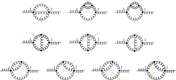
Figure 8: Diagrams for $\Pi_{11}^{a\mu,b\nu}$.

Figure 9: Diagrams for $\Pi_{21}^{a\mu,b\nu}$.

In order to cancel the above UV divergence, one needs to include the contributions from the diagrams in Figs. 8 and 9. The diagrams in Fig. 8 give

$$-i\bar{\Pi}_{11}(X,p)= -\frac{1}{8}\int_{p_{1},p_{2},p_{3}}(2\pi)^{4}\delta(p+p_{1}-p_{2}-p_{3})\overline{|M|^{2}}$$

$$\times[g_{22}(X,p_{1})-g_{22}(X,p_{2})-g_{22}(X,p_{3})].$$ (162)

And the diagrams in Fig. 9 yield

$$-i [\bar{\Pi}_{21}(X,p)-\bar{\Pi}_{12}(X,p)]=-\frac{1}{8}\int_{p_{1},p_{2},p_{3}}(2\pi)^{4}\delta(p+p_{1}-p_{2}-p_{3})\overline{|M|^{2}}.$$ (163)

Plugging (85), (89), (162) and (163) into the right-hand side of (160) gives the Boltzmann equation for gluons

$$p\cdot\partial f= \frac{1}{4}\int_{p_{1},p_{2},p_{3}}(2\pi)^{4}\delta(p+p_{1}-p_{2}-p_{3})\overline{|M|^{2}}$$

$$\times[f_{2}f_{3}(f+1)(f_{1}+1)-ff_{1}(f_{2}+1)(f_{3}+1)]$$ (164)

with $\overline{|M|^{2}}$ given in (86).

References

- (1) U. Heinz and R. Snellings, Collective flow and viscosity in relativistic heavy-ion collisions, Ann. Rev. Nucl. Part. Sci. 63 (2013) 123–151, [1301.2826].
- (2) S. Jeon and L. G. Yaffe, From quantum field theory to hydrodynamics: Transport coefficients and effective kinetic theory, Phys. Rev. D53 (1996) 5799–5809, [hep-ph/9512263].
- (3) F. Gelis, E. Iancu, J. Jalilian-Marian and R. Venugopalan, The Color Glass Condensate, Ann.Rev.Nucl.Part.Sci. 60 (2010) 463–489, [1002.0333].
- (4) Y. V. Kovchegov and E. Levin, Quantum Chromodynamics at High Energy. Cambridge University Press, 2012.
- (5) L. D. McLerran and R. Venugopalan, Computing quark and gluon distribution functions for very large nuclei, Phys. Rev. D49 (1994) 2233–2241, [hep-ph/9309289].
- (6) L. D. McLerran and R. Venugopalan, Gluon distribution functions for very large nuclei at small transverse momentum, Phys. Rev. D49 (1994) 3352–3355, [hep-ph/9311205].
- (7) L. D. McLerran and R. Venugopalan, Green’s functions in the color field of a large nucleus, Phys. Rev. D50 (1994) 2225–2233, [hep-ph/9402335].
- (8) Y. V. Kovchegov, Non-abelian Weizsäcker-Williams field and a two- dimensional effective color charge density for a very large nucleus, Phys. Rev. D54 (1996) 5463–5469, [hep-ph/9605446].
- (9) A. Ayala, J. Jalilian-Marian, L. D. McLerran and R. Venugopalan, Quantum corrections to the Weizsacker-Williams gluon distribution function at small x, Phys. Rev. D53 (1996) 458–475, [hep-ph/9508302].
- (10) Y. V. Kovchegov and D. H. Rischke, Classical gluon radiation in ultrarelativistic nucleus nucleus collisions, Phys. Rev. C56 (1997) 1084–1094, [hep-ph/9704201].
- (11) A. Krasnitz and R. Venugopalan, Non-perturbative computation of gluon mini-jet production in nuclear collisions at very high energies, Nucl. Phys. B557 (1999) 237, [hep-ph/9809433].
- (12) A. Krasnitz and R. Venugopalan, The initial energy density of gluons produced in very high energy nuclear collisions, Phys. Rev. Lett. 84 (2000) 4309–4312, [hep-ph/9909203].
- (13) A. Krasnitz, Y. Nara and R. Venugopalan, Probing a color glass condensate in high energy heavy ion collisions, Braz. J. Phys. 33 (2003) 223–230.
- (14) T. Lappi, Production of gluons in the classical field model for heavy ion collisions, Phys. Rev. C67 (2003) 054903, [hep-ph/0303076].
- (15) Y. V. Kovchegov, Can thermalization in heavy ion collisions be described by QCD diagrams?, Nucl. Phys. A762 (2005) 298–325, [hep-ph/0503038].
- (16) J. Berges, K. Boguslavski, S. Schlichting and R. Venugopalan, Universal attractor in a highly occupied non-Abelian plasma, Phys. Rev. D89 (2014) 114007, [1311.3005].
- (17) T. Epelbaum and F. Gelis, Pressure isotropization in high energy heavy ion collisions, Phys. Rev. Lett. 111 (2013) 232301, [1307.2214].
- (18) T. Epelbaum and F. Gelis, Fluctuations of the initial color fields in high energy heavy ion collisions, Phys. Rev. D88 (2013) 085015, [1307.1765].
- (19) J. Berges, K. Boguslavski, S. Schlichting and R. Venugopalan, Basin of attraction for turbulent thermalization and the range of validity of classical-statistical simulations, JHEP 05 (2014) 054, [1312.5216].
- (20) T. Epelbaum, F. Gelis and B. Wu, Nonrenormalizability of the classical statistical approximation, Phys. Rev. D90 (2014) 065029, [1402.0115].
- (21) T. Epelbaum, F. Gelis, N. Tanji and B. Wu, Properties of the Boltzmann equation in the classical approximation, Phys. Rev. D90 (2014) 125032, [1409.0701].
- (22) L. Kadanoff and G. Baym, Quantum Statistical Mechanics. W.A. Benjamin Inc., New York, 1962.
- (23) K.-c. Chou, Z.-b. Su, B.-l. Hao and L. Yu, Equilibrium and Nonequilibrium Formalisms Made Unified, Phys. Rept. 118 (1985) 1.
- (24) E. Calzetta and B. L. Hu, Nonequilibrium Quantum Fields: Closed Time Path Effective Action, Wigner Function and Boltzmann Equation, Phys. Rev. D37 (1988) 2878.
- (25) J.-P. Blaizot and E. Iancu, The Quark gluon plasma: Collective dynamics and hard thermal loops, Phys. Rept. 359 (2002) 355–528, [hep-ph/0101103].
- (26) P. B. Arnold, G. D. Moore and L. G. Yaffe, Effective kinetic theory for high temperature gauge theories, JHEP 01 (2003) 030, [hep-ph/0209353].
- (27) R. Baier, A. H. Mueller, D. Schiff and D. T. Son, ’Bottom up’ thermalization in heavy ion collisions, Phys. Lett. B502 (2001) 51–58, [hep-ph/0009237].
- (28) A. Kurkela and Y. Zhu, Isotropization and hydrodynamization in weakly coupled heavy-ion collisions, Phys. Rev. Lett. 115 (2015) 182301, [1506.06647].
- (29) A. H. Mueller and D. T. Son, On the Equivalence between the Boltzmann equation and classical field theory at large occupation numbers, Phys. Lett. B582 (2004) 279–287, [hep-ph/0212198].
- (30) J. S. Schwinger, Brownian motion of a quantum oscillator, J.Math.Phys. 2 (1961) 407–432.
- (31) L. Keldysh, Diagram technique for nonequilibrium processes, Zh.Eksp.Teor.Fiz. 47 (1964) 1515–1527.
- (32) N. P. Landsman and C. G. van Weert, Real and Imaginary Time Field Theory at Finite Temperature and Density, Phys. Rept. 145 (1987) 141.
- (33) M. L. Bellac, Thermal Field Theory. Cambridge University Press, 2011.
- (34) J. M. Cornwall, R. Jackiw and E. Tomboulis, Effective Action for Composite Operators, Phys. Rev. D10 (1974) 2428–2445.
- (35) J. Berges, N-particle irreducible effective action techniques for gauge theories, Phys. Rev. D70 (2004) 105010, [hep-ph/0401172].
- (36) J. Berges, Introduction to nonequilibrium quantum field theory, AIP Conf. Proc. 739 (2005) 3–62, [hep-ph/0409233].
- (37) M. E. Carrington, G. Kunstatter and H. Zaraket, 2PI effective action and gauge invariance problems, Eur. Phys. J. C42 (2005) 253–259, [hep-ph/0309084].
- (38) F. Gelis, T. Lappi and R. Venugopalan, High energy factorization in nucleus-nucleus collisions, Phys.Rev. D78 (2008) 054019, [0804.2630].
- (39) F. Gelis, T. Lappi and R. Venugopalan, High energy factorization in nucleus-nucleus collisions. II. Multigluon correlations, Phys.Rev. D78 (2008) 054020, [0807.1306].
- (40) S. Jeon, Color Glass Condensate in Schwinger-Keldysh QCD, Annals Phys. 340 (2014) 119–170, [1308.0263].
- (41) Y. V. Kovchegov and B. Wu, “Time-Dependent Observables in Heavy Ion Collisions II: in Search of Pressure Isotropization in the Theory.” in preparation, 2017.
- (42) A. H. Mueller, Small x Behavior and Parton Saturation: A QCD Model, Nucl. Phys. B335 (1990) 115.
- (43) Y. V. Kovchegov, Quantum structure of the non-Abelian Weizsäcker-Williams field for a very large nucleus, Phys. Rev. D55 (1997) 5445–5455, [hep-ph/9701229].
- (44) A. J. Niemi and G. W. Semenoff, Finite Temperature Quantum Field Theory in Minkowski Space, Annals Phys. 152 (1984) 105.
- (45) M. E. Peskin and D. V. Schroeder, An Introduction to quantum field theory. Addison-Wesley, Reading, USA, 1995.
- (46) Y. V. Kovchegov and M. D. Sievert, Sivers function in the quasiclassical approximation, Phys. Rev. D89 (2014) 054035, [1310.5028].
- (47) Y. V. Kovchegov and M. D. Sievert, Calculating TMDs of a Large Nucleus: Quasi-Classical Approximation and Quantum Evolution, Nucl. Phys. B903 (2016) 164–203, [1505.01176].
- (48) T. Lappi, Energy density of the glasma, Phys. Lett. B643 (2006) 11–16, [hep-ph/0606207].
- (49) K. Fukushima, Initial fields and instability in the classical model of the heavy-ion collision, Phys. Rev. C76 (2007) 021902, [0704.3625].
- (50) A. H. Mueller, The Boltzmann equation for gluons at early times after a heavy ion collision, Phys. Lett. B475 (2000) 220–224, [hep-ph/9909388].
- (51) J. D. Bjorken, Highly relativistic nucleus-nucleus collisions: The central rapidity region, Phys. Rev. D27 (1983) 140–151.
- (52) Y. V. Kovchegov and H. Weigert, Collinear Singularities and Running Coupling Corrections to Gluon Production in CGC, Nucl. Phys. A807 (2008) 158–189, [0712.3732].
- (53) V. Mathieu, A. H. Mueller and D. N. Triantafyllopoulos, The Boltzmann Equation in Classical Yang-Mills Theory, Eur. Phys. J. C74 (2014) 2873, [1403.1184].
- (54) T. Epelbaum, F. Gelis and B. Wu, Lattice worldline representation of correlators in a background field, JHEP 06 (2015) 148, [1503.05333].
- (55) T. Epelbaum, F. Gelis and B. Wu, From lattice Quantum Electrodynamics to the distribution of the algebraic areas enclosed by random walks on , 1504.00314.