Dynamics and flow effects in the Beris-Edwards system
modeling nematic liquid crystals
Abstract
We consider the Beris-Edwards system modeling incompressible liquid crystal flows of nematic type. This couples a Navier-Stokes system for the fluid velocity with a parabolic reaction-convection-diffusion equation for the -tensors describing the direction of liquid crystal molecules. In this paper, we study the effect that the flow has on the dynamics of the -tensors, by considering two fundamental aspects: the preservation of eigenvalue-range and the dynamical emergence of defects in the limit of high Ericksen number.
1 Introduction
In this paper we consider the Beris-Ewdards system modelling nematic liquid crystals [9]. It is one of the main PDE systems modeling nematic liquid crystals in the -tensor framework and one of the best studied mathematically [1, 2, 36, 37, 21, 22, 41]. It couples a Navier-Stokes system for incompressible flow with anisotropic forces and a parabolic reaction-convection-diffusion system for matrix-valued functions, i.e., the -tensors. The Navier-Stokes system captures the fluid motion and the reaction-convection-diffusion system describes the evolution of the liquid crystal director field (see Section 2 for physical aspects).
In the Landau-de Gennes theory of liquid crystals (see [16, 33, 30]), the local orientation and degree of order for neighboring liquid crystal molecules are represented by a symmetric, traceless matrix that is an element of the -tensor space:
| (1.1) |
The physical interpretation of the space of -tensors is presented for instance in [30].
The system we are focusing on involves a number of physical constants. For the purpose of our study it is convenient to set most of these constants equal to one, keeping just a couple of specific interest to us. A specific non-dimensionalisation will be provided in Section 2.2. In the rest of the paper, we will focus on the Beris-Ewdards system written in a non-dimensional form as:
| (1.2) | |||
| (1.3) | |||
| (1.4) |
where
Here, we denote by the two dimensional torus. Then represents the fluid velocity field and stands for the liquid crystal directors, with , being the symmetric and skew-symmetric parts of the rate of strain tensor, respectively. The constant in is a measure of the ratio between the tumbling and the aligning effects that a shear flow exerts on the liquid crystal director field.
There has been a vast recent literature on the study of well-posedness as well as long-time dynamics of the Beris-Edward system (1.2)–(1.4). We refer interested readers to [2, 13, 12, 21, 22, 37] for the discussion related to the simplified system with , and [1, 11, 14, 36] for the full system with a non-vanishing .
The system (1.2)–(1.4) contains a significant number of terms and generates considerable analytical difficulties, mostly due to the presence of the Navier-Stokes part that describes the effects of the fluid. Often in the physical literature it is assumed that the fluid can be neglected and one works with some suitably simplified fluid-free versions of the system. However, it is not a priori clear what is lost through these simplifications and the main aim of this work is to study two interlinked fundamental issues:
-
•
The preservation of eigenvalue-range,
-
•
The partial decoupling in the limit of high Ericksen number.
We aim to provide an understanding of these qualitative issues. Thus, in this paper we will focus on the simplest possible setting, from a technical point of view, that allows to bypass regularity issues (in particular, for the Navier-Stokes system). Namely, we will work on the two dimensional torus and with sufficiently smooth solutions, i.e., the global strong solutions. The existence of global strong solutions in this setting for the full system (1.2)–(1.4) was done in [11], however assuming that the range of -tensors is the set of two dimensional tensors, i.e. matrices. The framework we use here is slightly different such that we work essentially in a three dimensional setting for the target spaces (cf. [36, Remark 1.1]). More precisely, we consider the fluid velocity and the -tensor defined on but take values in the spaces and (see (1.1)), respectively. This setting can be easily obtained from the work in [11] by assuming that we work in three dimensional space with initial data independent of one spatial direction, so essentially a two dimensional datum (in the domain). This property of the initial data of being two dimensional is preserved by the flow and all the arguments in [11] follow, because the only thing that matters for obtaining global strong solutions is the Sobolev embedding theorem that continues to hold as the domain is kept to be essentially two dimensional. Hence, we shall simply assume the existence of global strong solutions defined as follows:
Definition 1.1.
The first issue of interest to us, i.e., the preservation of eigenvalue-range, concerns the behaviour of eigenvalues of -tensors under the fluid dynamics. The main question is to understand what will happen as time evolves if the eigenvalues of the initial datum are in a convex set (with in the current stage): will they stay in the same set or not? As explained in the next section this is a fundamental issue motivated by the physical interpretation of the -tensors.
It is already known (see for instance, [22, Theorem 3]) that if one takes in the system (1.2)–(1.4), then a maximum principle is valid for the -equation, i.e., the -norm of the initial datum will be preserved for the solution during the evolution. However, as pointed out in [27] the preservation of eigenvalue-range is a much more subtle issue than the preservation of -norm of .
On the other hand, if the fluid is neglected, i.e., , then the -equation (1.4) is simply reduced to a gradient flow of the free energy (see (2.1) for its definition). It is proved in [27] (in the whole space setting) that this gradient flow will preserve the convex hull of eigenvalues of for any regular solution . The proof therein is based on an operator splitting idea and a nonlinear Trotter product formula [40]. More precisely, the gradient flow is “splitted” into a heat flow and an ODE system so that the initial eigenvalue constraints are shown to be preserved by both sub-flows. Then the Trotter formula performs the combination. Returning to our full system (1.2)–(1.4), we note that the structure of the current -equation is nevertheless much more complicated such that the argument for the heat flow part in [27] can no longer be applied. To overcome the corresponding mathematical difficulty, we shall introduce a singular potential discussed in [5] (see [18, 19, 23, 41] for various applications), and make a thorough exploration of its special properties.
To this end, we will first investigate the special case . In the literature this is often referred to as the “co-rotational case”. Taking generates considerably simpler equations and in particular, ensures the validity of a maximum principle for . In this special case, we will show that in fact one even has the preservation of a suitable convex eigenvalue-range and thus extending the results in [27] to the current case with flow. As mentioned in [27], the preservation of -norm of (i.e., the maximum principle) can be viewed as a “weaker” version of the preservation of physicality (i.e., the preservation of eigenvalues).
Theorem 1.1.
[Eigenvalue preservation in the co-rotational case ]. Let , , , , , and with . We assume that the eigenvalues of the initial datum satisfy
| (1.5) |
Furthermore, we impose the following restriction on the coefficients:
| (1.6) |
Let be the global strong solution to the system (1.2)–(1.4) on with initial data . Then for any and , the eigenvalues of stay in the same interval as in (1.5).
We infer from Theorem 1.1 that for our system (1.2)–(1.4) the fluid velocity field will not affect the initial eigenvalue constraint on as time evolves, provided that .
On the other hand, generally one cannot prove any maximum principle of for the full system (1.2)–(1.4) unless . Next, we will show that for the general case with , the preservation of eigenvalues indeed does not hold as well. For this purpose, we will argue by contradiction and use a simplified version of the full system (1.2)–(1.4). This will be obtained as the so-called high Ericksen number limit, which corresponds to the formal limit in our setting. The resulting system we obtain is only weakly coupled, namely, it is a system coupling an Euler equation for the fluid velocity with a reaction-convection equation for the order parameter . First, we prove
Theorem 1.2.
[High Ericksen number limit in the co-rotational case]. Let with and . Consider the “limit system”:
We note that the assumption in the above theorem can be removed, provided that one has an a priori -bound of that is also uniform in . On the other hand, if we assume that the property of eigenvalue preservation holds, then we actually have such an a priori -bound. As a consequence, we can obtain the limit system (1.7)–(1.9) in the non co-rotational case i.e., , for which we can show that in general one cannot except the preservation of the initial eigenvalue range. This is the overall basic strategy leading to our next result:
Theorem 1.3.
[Lack of eigenvalue preservation in the non co-rotational case].
Finally, in Section 6 we return to the system obtained in the limit of high Ericksen number with , i.e., (4.1)–(4.3). As argued in the physical motivation in Section 2, this is relevant for understanding certain patterns, specific to liquid crystals, the “defect patterns” (see [16]). We consider certain specific solutions of the Euler equations and provide examples of flows that are non-singular but are still capable of generating various types of such defect patterns. More precisely, we present two distinct way of generating defects: the phase mismatch in absence of the flow and these vorticity-driven defects.
The rest of this paper is organized as follows. In the next section we provide a couple of background details concerning the physical relevance of our study. This is a section that the mathematically-minded readers can safely skip. Then in Section 3 we provide the proof of Theorem 1.1 concerning the preservation of eigenvalue-range in the co-rotational case with . In Section 4, we obtain the limit of high Ericksen number and prove the error estimates, i.e., Theorem 1.2. Then in Section 5, we can use the reduced system to argue for the initial system that for we cannot always have eigenvalue preservation, thus proving Theorem 1.3. Finally, in Section 6 we return to the reduced system with and study its implications concerning the dynamical appearance of defect patterns. In the Appendix, we recall some rather technical results that are necessary in Sections 3 and 6 but that seem difficult to pinpoint in the literature.
Notational Conventions
Throughout the paper, we assume the Einstein summation convention over repeated indices. We define for matrices , and denote by the Frobenius norm of the matrix such that . Besides, the identity matrix will be denoted by . The partial derivative with respect to spatial variable of the -component of is denoted by or . Next, we define the matrix valued space () by
For the sake of simplicity, unless explicitly pointed out, we shall simply use to express for the fluid velocity and for the -tensors. In a similar manner, we use () to represent the Sobolev spaces for the fluid velocity and for -tensors, respectively. We will at times abbreviate as , as etc.
2 Physical aspects
2.1 Eigenvalue-range constraints
The main characteristic of nematic liquid crystals is the locally preferred orientation of the nematic molecule directors. This can be described by the -tensors, that are suitably normalized second order moments of the probability distribution function of the molecules. More precisely, if is a probability measure on the unit sphere , representing the orientation of liquid crystal molecules at a point in space, then a -tensor denoted by is a symmetric and traceless matrix defined as
It is supposed to be a crude measure of how the probability measure deviates from the isotropic measure where , see [30]. The fact that is a probability measure imposes a constraint on the eigenvalues of such that (see [30])
Thus, not any symmetric and traceless matrix is a physical -tensor but only those whose eigenvalues take values in .
2.2 Non-dimensionalisation and the Ericksen number
The free energy of liquid crystal molecules is given by
| (2.1) |
where , , , are material dependent and temperature-dependent constants that satisfy [33, 34]
| (2.2) |
Here, we use the one constant approximation of the Oseen-Frank energy for the sake of simplicity (see [5]).
The Beris-Edwards system we are going to consider is given by
| (2.3) | |||
| (2.4) | |||
| (2.5) |
Here represents the fluid velocity field and stands for the -tensor of liquid crystal molecules. The positive constants and denote the fluid viscosity and the macroscopic elastic relaxation time for the molecular orientation field, respectively.
In the -equation (2.5), the tensor is defined to be the minus variational derivative of the free energy with respect to under symmetry and tracelessness constraints:
| (2.6) |
meanwhile the term in (2.5) reads as follows
| (2.7) |
where and stand for the stretch and the vorticity tensor, respectively. It is worth pointing out that the constant in (2.7) is a measure of the ratio between the tumbling and the aligning effects that a shear flow exerts on the liquid crystal director field.
Next, the anisotropic forcing terms in the Navier-Stokes system (2.3) are elastic stresses caused by the presence of liquid crystal molecules, which include the symmetric part
| (2.8) |
and the skew-symmetric part
| (2.9) |
Thus, the coupled system (2.3)–(2.5) takes the following explicit form:
| (2.10) | |||
| (2.11) | |||
| (2.12) |
Besides, we assume the system (2.10)–(2.12) is subject to the initial conditions
| (2.13) |
The full system (2.10)–(2.13) involves several dimensional parameters (see [6, 38] and the references therein):
-
•
is the density (assumed to be constant here), expressed in units of .
-
•
is an elastic constant, measuring spatial distortions of the order parameter , expressed in units of ,
-
•
, and are material-dependent parameters (at a fixed temperature), expressed in units of ,
-
•
is the fluid viscosity, expressed in units of ,
-
•
is the inverse of a viscosity coefficient, expressed in units of .
We remark that the parameter is a non-dimensional constant measuring a characteristic of the molecules.
Following the non-dimensionalisation performed in [29], we denote the characteristic length, velocity and density by , , , respectively. Then we define the non-dimensional distance and time as:
Take the non-dimensional variables , , and to be such that:
Inserting the above relations into the system (2.10)–(2.12), we obtain
| (2.14) | |||
| (2.15) | |||
| (2.16) |
where and .
On the other hand, we recall that the non-dimensional Ericksen and Reynolds numbers can be defined as follows (see [29]):
| (2.17) |
| (2.18) |
Furthermore, we introduce the following non-dimensional quantities:
which implies that the system (2.14)–(2.16) becomes, in a non-dimensional form:
| (2.19) | |||
| (2.20) | |||
| (2.21) |
Remark 2.1.
Taking into account the definitions (2.17), (2.18) for the Ericksen and Reynolds numbers we see that the physical parameters , are material-dependent, hence fixed, and we can only vary or . We observe that is essentially a unit of the length measurement, which can be changed for instance from meters to meters. Hence, formally increasing amounts to obtaining a system relevant on a much larger scale. Similarly, fixing and changing amounts to a change of scale in time. The most important thing to notice is that a change of scale implies a simultaneous change in all the non-dimensional parameters.
In order to study defect patterns, which appear as localized high gradients, it is useful to take a large space scale for fixed time scale (which also implies that and is fixed). This corresponds to taking large Ericksen and Reynolds numbers, simultaneously:
| (2.22) |
where is a parameter that will be sent to .
In the remaining part of the paper, we focus on the scaling (2.22) and for notational simplicity, we set
Dropping the bars of unknown variables and the spatial/temporal variables, setting without loss of generality, the system we are going to study becomes the one in the introduction, namely (1.2)–(1.4).
3 Eigenvalue-range preservation in the co-rotational case
In this section, we aim to prove Theorem 1.1. To this end, we consider the system (1.2)–(1.4) with . Assume that is a strong solution to this system, existing on some time interval . Below we will investigate the -equation (1.4) only, regarding the velocity (and thus ) in the convection terms as given and sufficiently smooth functions. In Subsection 3.2, we will show that this smoothness assumption can be relaxed in certain sense. Then the proof of Theorem 1.1 will be obtained in the last subsection of this section, by using a nonlinear Trotter product formula whose mechanism is explained in an abstract setting in the Appendix, Section A (see [40] for the autonomous case).
3.1 Eigenvalue-range preservation for decomposed systems
To begin with, we denote by , or the flow generated by the ODE part of (1.4), i.e., satisfies the ODE system
| (3.1) |
Consider the convex set (see for instance [10] for a proof of its convexity)
| (3.2) |
It has been shown in [27] that the solution to (3.1) always lies in this set provided that its initial datum lies in (3.2) (for details, see Step 2 of the proof of [27, Proposition 2.2]).
On the other hand, for , we denote the unique solution to the linear non-autonomous problem
| (3.3) |
where is a given divergence-free function in and . Next, we prove that the two parameter evolution system defined by problem (3.3) also preserves the above closed convex hull of the range for the initial data.
Denote
Similar to the singular potential of Ball–Majumdar type considered in [5], for every fixed (sufficiently small) , we take
| (3.4) |
where the admissible set is given by
According to [5], for a given , we minimize the entropy term over all probability distributions that have a fixed normalized second moment . Define the bulk potential
Namely, the minimization over the set is only defined for those -tensors that can be expressed as the normalized second moment of a probability distribution function and whose eigenvalues obey the above physical constraints. Similarly to [23], one can easily check that
-
•
is strictly convex.
-
•
is smooth in , i.e., when
-
•
is isotropic, i.e.,
Remark 3.1.
Now consider the linear equation (3.3) on . Let be defined as follows
We claim that
This conclusion can be justified by a contradiction argument. Suppose , we see that for . Taking the (matrix) inner product of equation (3.3) with yields
Since , then by (3.1) we see that the above equation can be reduced to
| (3.7) |
where in the last step we used the convexity of .
Hence, the maximum principle for together with the assumption (1.5) on the initial eigenvalue-range for gives
The strict physicality property of (in a similar manner as in [5, Theorem 1]) indicates that there exists
This however leads to a contradiction with the definition of .
As a consequence, we conclude that and
Since is arbitrary, after performing a continuity argument we can obtain that
3.2 Eigenvalue-range preservation under weaker regularity
We show that the previous eigenvalue-range preservation property may still hold for solutions with weaker regularity (even weaker than what we actually need).
Proposition 3.1.
Let , , be such that
Assume that is the unique solution of the system
and satisfies
| (3.8) |
where denote the increasingly ordered eigenvalues of .
Then a.e. in as , where is the unique solution in of the system
Moreover, we have an eigenvalue constraint on (provided that its initial datum also has the same constraint):
| (3.9) |
Proof.
First, we prove an a priori -bound for . Since , there exists a positive number such that for any ,
Then we take . Multiplying (3.1) by and integrating over , after integration by parts, we obtain
which implies
| (3.10) |
In a similar manner, we can obtain the same result for
| (3.11) |
Denote the difference . Then satisfies the following equation
Multiply the above equation by and integrating over , after integration by parts and taking into account the uniform -bounds on , and also , respectively (see (3.10), (3.11)), we get
where a constant depending only on and . Thus, it holds
From our assumptions, we know that
as . Then we can conclude
| (3.12) |
Thus, for any time , we get a.e. in and thanks to the continuity of eigenvalues as functions of matrices (see, for instance [35]) we obtain the claimed bounds on the eigenvalues of . The proof is complete. ∎
3.3 Proof of Theorem 1.1
We are in a position to prove Theorem 1.1. Returning to equation (1.4), we assume for now , a regularity assumption that will be eventually removed thanks to the previous subsection. For some time , and , we denote
and . Furthermore, we define
| (3.13) |
for .
Recalling the Trotter product formula, in its abstract form as in Proposition A.1 in the Appendix, we choose
and
Below we proceed to verify the assumptions (H1)–(H2) made in Proposition A.1 under the above choices.
First, we can easily see that the solution operator of the ODE system (3.1) fulfills the assumption (H2) on its existence interval .
Next, for , the existence of the evolution system associated with the linear parabolic problem (3.3) with initial datum can be easily verified. Then it remains to verify the assumption (H1).
Let be solution to (3.3) with initial datum . Multiplying both sides of equation (3.3) with and integrating over , we have
where we used the facts that and . Thus,
| (3.14) |
Multiplying both sides of equation (3.3) with and integrating over , we have
where the constant depends on and . As a result, we can easily deduce from Gronwall’s lemma that
which implies
| (3.15) |
We note that the solution can be written as
We recall a simple and rather standard estimate for the heat equation. To this end, we decompose any function as where form a complete orthonormal system in of eigenvectors of the minus Laplacian, with corresponding eigenvalues ordered in a non-decreasing sequence. Then we have and . It easily follows that
| (3.16) |
Using the above estimate and the uniform estimate of , we obtain
| (3.17) |
We recall estimate (3.14), which together with the simple fact on
and the last estimate implies
| (3.18) |
Let
We deduce from the above integral inequality that
| (3.19) |
where
On the other hand we have:
As a consequence, by Gronwall’s lemma, we obtain
which implies that
Combing the above estimate with (3.14), we infer that
| (3.20) |
Next, we have the following estimate
where may depend on . The last estimate implies
On the other hand, from (3.15) we already know
Hence, from the interpolation inequality for any , we easily conclude that
| (3.21) |
In view of the estimates (3.15), (3.20) and (3.21), the evolution system satisfies (A.5). Thus, the assumption (H1) is verified.
In summary, we are able to apply Proposition A.1 to conclude that
| (3.22) |
On the other hand, we observe that can be viewed as the successive superpositions of solutions of the ODE part (3.1) and the second order parabolic equation part (3.3) with specific initial data. As a consequence, since we have already known that both operators and preserve the closed convex hull of the range of the initial data, then the proof of Theorem 1.1 can be accomplished by passing to the limit in (3.13), which is guaranteed by the estimate (3.22) (where thanks to the previous subsection we do use the result on eigenvalue preservation for at the level of regularity on that is guaranteed by the strong global solutions).
The proof of Theorem 1.1 is complete.
Remark 3.2.
Theorem 1.1 is still valid if the two dimensional torus setting is replaced by the whole space.
4 Large Ericksen number limit in the co-rotational case
In this section we prove Theorem 1.2. To this end, we denote by the solution of the limit system obtained by formally setting in the system (1.2)–(1.4) with . Hence, it satisfies the following weakly coupled system:
| (4.1) | |||
| (4.2) | |||
| (4.3) | |||
| (4.4) |
where .
Since it is assumed that , thanks to the regularity theory for Euler equation we have (see e.g. [28]). Next, by standard results for transport equation on the torus with , due to the assumption on the initial datum and the aforementioned regularity of , we are able to deduce (see Proposition B.1 in the Appendix for further details).
For any , we denote the global strong solution to system (1.2)–(1.4) with , subject to the initial data and .
Set
Then the difference functions satisfy the following system (dropping the superscript for the sake of simplicity):
| (4.5) |
where and
We multiply the third equation in (4.5) for by , integrate over , take the trace and sum with the first equation in (4.5) multiplied by and integrated over . After integration by parts and taking into account the cancellations at the energy level, we obtain
| (4.6) | |||
| (4.7) |
Using [2, Lemma 2.1] and the incompressibility condition, one can easily check that
as well as
Then using the Hölder inequality and Young’ inequality, we can estimate the remaining terms on the right-hand side of (4.7) as follows:
| (4.8) |
where is a positive constant independent of .
Denote
It follows from (4.8) and the Cauchy–Schwarz inequality that
where is a constant independent of .
From our assumption, we infer that , and are uniformly bounded on for . Since , it follows from Gronwall’s lemma that for
The proof of Theorem 1.2 is complete.
5 Lack of eigenvalue-range preservation in the non-corotational case
5.1 The high Ericksen number limit in the non-corrotational case
As a first step for the proof of Theorem 1.3, we prove an analogue of Theorem 1.2 by assuming that a uniform a priori -bound for is available (see (5.5)). This assumption will be satisfied if we impose certain bound on the eigenvalues of (for instance, (5.9) below) in the subsequent contradiction argument.
Proposition 5.1.
[High Ericksen number limit in the non co-rotational case].
Proof.
The proof is basically an extension of the one for the co-rotational case in Section 4, which however is more involved since . The reader can safely skip to continue with the proof of Theorem 1.3 in the next subsection.
Like before, since , thanks to the regularity theory for Euler equation we have (cf. [28]). By standard results for transport equation on the torus with , due to the assumption on the initial datum and the aforementioned regularity of , we are able to deduce (See Proposition B.1). We remark that here the fact does not introduce any extra difficulty.
For any , we denote the global strong solution to system (1.2)–(1.4) with , subject to the initial data and .
Set
We see that satisfies the following system (dropping the superscript for the sake of simplicity):
| (5.6) |
where , and
We multiply the third equation in (5.6) for by , integrate over , take the trace and sum with the first equation in (5.6) multiplied by and integrated over . After integration by parts and taking into account the cancellations at the energy level, we obtain
Again using [2, Lemma 2.1], the incompressibility condition and the fact , one can verify that
as well as
Then using the Hölder inequality and Young’ inequality, we can estimate the remaining terms on the right-hand side as follows:
| (5.7) |
where the constant is independent of and .
Let
From the definition of , it easily follows that with some independent of . Then using the Cauchy–Schwarz inequality, we infer from (5.7) that
where is a constant that may depend on but is independent of .
Since , are a priori bounded (in particular is now assumed to be bounded), from the fact and Gronwall’s lemma, we deduce that for , it holds
The proof is complete. ∎
5.2 Proof of Theorem 1.3
We are in a position to prove Theorem 1.3. This can be done by a contradiction argument. To this end, we assume that if
| (5.8) |
then for any , , , , and any , we still have the eigenvalue-range preservation:
| (5.9) |
Since the physicality of a -tensor imposes an upper bound on the size of , then thanks to the bound on eigenvalues (5.9), we see that (5.5) is satisfied with certain . As a consequence, from Proposition 5.1 we infer that the limit system as i.e., (5.1)–(5.4), also has the eigenvalues in the same range (because pointwise convergence of -tensors implies pointwise convergence for their eigenvalues, as eigenvalues are continuous functions of matrices, see for instance [35]).
Next, we recall the equation
| (5.10) |
where is a solution of the Euler equation (5.1). Since and , we know that and . Now we define
and then the pair satisfies the following system
Applying the curl operator to the first equation, we see that satisfies
Since , we infer that there exists certain constant independent of such that , provided that . Hence, we deduce that as
where is the initial data for the velocity field.
Moreover, we have as uniformly for and , where solves the ODE system (parametrized by ):
where . If we take the initial datum , we will have, as long as the matrix then the solution , namely, there exists some such that .
As a consequence, there exists a sufficiently small (depending on this nonzero ) such that if we take the coefficients
that satisfy
we have
but for , it holds
This leads to a contradiction, which proves our assertion.
The proof of Theorem 1.3 is complete.
6 Dynamical emergence of defects
In this section, we investigate some qualitative features of solutions to the system (i.e., the “limit system” of (1.2)–(1.4) with ):
| (6.1) | |||
| (6.2) | |||
| (6.3) |
Our aim is to understand how it can describe liquid crystal defects that are understood as high gradients. We shall provide some specific examples of flows providing mechanisms responsible for this phenomenon, which can be regarded as the generation of defect patterns.
As has been seen in the previous sections, the equation for is well-posed in the spaces in which we work, so if one starts with then for (see for instance, Proposition B.1 in the Appendix). However, what can happen is that for certain types of initial data the -norm of the gradients of can increase in time on the interval . Below we present two distinct ways of generating defects:
-
•
phases mismatch;
-
•
vorticity-driven defects.
6.1 The phases mismatch
We first consider the case when the flow is not present, namely, . Then the equation (6.3) reduces to the gradient flow of an ODE system:
| (6.4) |
whose solutions evolve in time towards one of the two stable minima, namely, the local minimum , respectively the global minimum . Here,
with , . More specifically, one can easily check that if we take for instance
where , then the solution of (6.3) will be with
Therefore, as the gradient of at the plane will increase towards infinity as .
6.2 Vorticity-driven defects
Given the roughness specific to Euler equation, one can expect that defects are related to discontinuities and high gradients in the flow. However, this is not the only possible mechanism. Indeed, we will show that even for a very well-behaved flow, e.g., a stationary flow we are able to get for generic points that the gradients of the -tensor will increase in time.
Below we consider two cases that are in some sense extreme: (1) a very general flow, but very specific initial data, and (2) a very general initial datum, but with more restrictions on the flow.
6.2.1 General flow and special initial data
We have the following:
Proposition 6.1.
Let be a stationary solution of the incompressible Euler system in . We denote by its vorticity, namely and assume that there exists a sequence with as and , for all . We further assume that , and let , with and .
Then, denoting , and letting be an initial datum for equation (6.3) with the given flow , we see that there exists a sequence of times and points (with in the segment connecting and ) such that
Remark 6.1.
For all non-degenerate critical points of the vorticity one can choose an approximating sequence in a subset such that is a non-degenerate local extremum, hence the assumption , for all is satisfied.
Proof.
We consider a Lagrangian perspective. Recall that for the given flow , the corresponding particle-trajectory map is defined as the solution of the following ODE system:
| (6.5) |
Since the torus is a compact manifold, the solution exists for .
We can thus now rewrite (6.3) as an ODE along particle paths:
| (6.6) |
where the matrix is related to the vorticity of the fluid, namely
| (6.7) |
Furthermore, because the flow is , the vorticity is constant along particle paths (see for instance, [32, Corollary 1.2]):
| (6.8) |
In order to further simplify the equation (6.6), we introduce the operator as the solution of the following system:
| (6.9) |
Lemma 6.1.
is a rotation operator, i.e., , and .
Proof.
Note that
Let . We see that is a solution of the ODE system
It is obvious that is also a solution of this linear system, then by uniqueness we have
which yields the conclusion. ∎
Thanks to the rotation operator , we can further derive
Lemma 6.2.
Proof.
Denote
Then the system (6.6) becomes
| (6.10) |
We know that the equation (6.10) satisfied by is a gradient flow, hence except for the case when one start with zero initial data, in the long-time we will have evolution to one of the two manifolds of steady states, namely,
Moreover, taking the initial data in one of these two manifolds, as we do by the initial assumptions, we have that the solution is stationary in time, hence , which in terms of becomes:
The proof is complete. ∎
Because the flow is defined for all real times, in terms of we infer from the above lemma that
where
| (6.11) |
On the other hand, taking into account the definition (6.9) of , we have
where for the last equality we used the formula for the exponential of a matrix (see for instance, [24]). Using the fact that in the vorticity is conserved along the flow map (6.8), we have
Hence, (6.11) becomes
Taking and , respectively, we can calculate the angle between the two vectors at these points, at times (to be fixed later) as
Recalling now the assumption in the hypothesis that , we can take the times
As a consequence, we have that as the angle between and stays non-zero and fixed, as . This leads to the final claim of the proposition. ∎
6.2.2 General initial data and special points in the flow
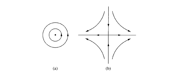
In dimension two, a divergence-free flow can be expressed in terms of a stream function. More precisely, if is smooth enough with and moreover then there exists a scalar function , called the stream function, such that . Thus the system providing the particle-trajectory map (6.5) becomes a Hamiltonian flow, and the stagnation points of the flow are given as critical points of the stream function . Locally, the flow around them will be as in Figure 1 (see for instance, [20, Chapter 1]).
We will need to assume essentially that around such points the vorticity is not constant, namely we have the kind of assumption of non-degeneracy imposed in Proposition 6.1. We expect that this kind of assumption holds generically, so we will call these “standard stagnation points”. More precisely,
Definition 6.1 (Standard stagnation points in incompressible flows).
Consider an incompressible flow with zero mean. We call a standard stagnation point for the flow , if and there exists a sequence of points with such that , uniformly for and for any (where is the particle-trajectory map generated by the flow and is the vorticity of the flow).
Then we have the following:
Proposition 6.2.
Let be a stationary solution of the incompressible Euler system with zero mean. Let be a standard stagnation point in the sense of Definition 6.1 and be a function such that is a biaxial -tensor that belongs to a suitable neighborhood of the set (as defined in Proposition C.1 in the Appendix).
Then there exist a sequence of points converging to and a sequences of times such that
Proof.
We consider, similarly as in the proof of Proposition 6.1, the particle-trajectory map , generated by the flow . Then following the reasoning in the proof of Proposition 6.1 we obtain:
where (with ) is the long-time limit of the gradient flow (6.10) starting from initial data (see Proposition C.1 in the Appendix).
Thanks to the assumption that is a standard stagnation point (see Definition 6.1), we deduce that there exists a sequence of points converging to such that
and
| (6.12) |
On the other hand, we have
On a simply-connected neighbourhood of of we can define the “angle function” depending on the function such that for all . Taking into account that is a continuous function on the neighbourhood (see Proposition C.1 in the Appendix), the angle function (or its lifting in topological jargon) can be chosen to be continuous.
Thus, with this notation we obtain
where
Because of (6.12), we can take
Then, using the continuity of the angle function we deduce that as .
The proof is complete. ∎
Appendix A The nonlinear Trotter product formula
Suppose is a solution to the parabolic problem
| (A.1) |
One can obtain its solutions by successively solving two simpler equations
| (A.2) |
Such Trotter product formulas combining the solutions of the two simpler equations are available in the literature in the case when is a time-independent operator (see for instance, [40]). However, such results do not seem to be immediately available in the literature for time-dependent operators as we need. So we provide here a brief argument showing the specific result we shall use, which follows closely the argument in [40, Proposition 5, pp. 310].
We start by recalling the following definition (cf. [39], pp. )
Definition A.1.
Let be a Banach space. The two-parameter family of bounded linear operators for on is called an evolution system if:
(i) , for any ;
(ii) the mapping is strongly continuous for .
Then we denote by the evolution system generated by the time-dependent operator on the Banach space . Besides, we also let be the one-parameter semigroup generated on by the nonlinear ODE .
For , , , we set
| (A.3) |
and furthermore
| (A.4) |
Proposition A.1.
Let and be two Banach spaces such that is continuously embedded in . We make the following assumptions.
(H1) Suppose that the evolution system generated by on satisfies
| (A.5) |
for , with some , . Here, stands for the identity operator and denotes the set of bounded linear operators from into .
(H2) Let be the flow generated by the vector field . Assume it satisfies:
for . Here, are some constants independent of .
We also assume that
| (A.6) |
where
Proof.
The proof is adapted from that of [40, Proposition 5.1]. We note that for ,
where
We infer from the assumptions (H1), (H2) the following estimates
and
Let . Then the difference satisfies the equation
Using Duhamel’s principle (see [39]), we know that
As a consequence, by assumptions (A.5)–(A.6) and the definition of , we obtain
| (A.7) |
Hence, the proof is complete by a direct application of Gronwall’s Lemma to the inequality (A.7). ∎
Appendix B Global existence for the limit system
In order to provide the global existence for the limit system as , we first recall some technical result, concerning estimates in higher order space, in particular the commutator estimates, that are nowadays standard (see for instance, [31]).
Lemma B.1.
For any (, ) and any multi-index with , we have
| (B.1) | |||
| (B.2) |
for some positive constant independent of .
We can now provide our global existence result:
Proposition B.1.
Consider the following system for and :
| (B.3) | |||
| (B.4) | |||
| (B.5) |
with and .
Proof.
For the Euler system it is well known that if then there exists a global solution in the same space, with values in . In our case we take values in , so for the third component indeed we have a transport equation with a Lipschitz velocity (provided by the first two components). Hence, by standard results we also have that the solution stays in the same space as the initial datum.
For the -part, we just provide a priori estimates, leaving the approximation procedure to the interested reader. Multiplying the equation (B.5) by () and integrating by parts, we obtain:
| (B.6) |
On the other hand, noting that can be expressed in terms of eigenvalues one can check that we have for any the estimate: , which implies:
Furthermore, we have
Using the above two estimates in (B.6), we get
Since , we deduce that
Thus, out of the above nequality, using Gronwall’s inequality, the a priori estimate on and passing to the limit we get
| (B.7) |
We take now the scalar product in of (B.5) with and obtain
| (B.8) |
We estimate each term on the right-hand side separately.
where we used the estimate (B.2) in the last inequality. Then for the second term we use repeatedly the estimate (B.1) to get
Furthermore, for the third term, we have
A similar arguments lead to:
Gathering the above estimates and using them in (B.8), we obtain
Taking into account that and are controlled a priori in , then using Gronwall’s lemma, we deduce the desired a priori control of in .
The proof is complete. ∎
Appendix C Local ODE dynamics
Consider the ODE system
| (C.1) |
Then we have
Proposition C.1.
Let the coefficients of system (C.1) satisfy , . Denote by
the set of stationary points of the equation (C.1).
There exists a neighbourhood of , within the set of all -tensors, such that for any the ODE system (C.1) starting from the initial datum will evolve in the long time towards , with the function and continuous at all biaxial points in .
Proof.
We start by recalling the argument from [27] that the dynamics of the ODE system (C.1) affects only the eigenvalues, but not the eigenvectors. Indeed, let us consider “the system of eigenvalues”:
| (C.2) |
Using standard arguments it can be shown that the system (C.2) has a global-in-time solution .
For an arbitrary initial datum , since is a symmetric matrix, there exists a matrix , such that where are the eigenvalues of . It can be shown (see [27] for details) that
with being the solution of the ODE system (C.2) subject to the initial data .
Therefore, for close to , we have (taking into account that the eigenvalues are a continuous function of the matrix, see for instance [35]) that its eigenvalues are close to , and , respectively. Thus, there exists a matrix , such that where is small.
Denote . A straightforward calculation shows that the Hessian matrix at is given by
Its eigenvalues take the following form
which can be checked to be negative under the assumption on and . Thus, the standard ODE theory (see for instance,[20]) implies that for initial data in a neighbourhood of , we have that in the long time the solution will converge exponentially to . Let us denote by this neighbourhood.
We denote
which is a neighbourhood of . We can see that the solution of the ODE system (C.1) starting from will evolve in the long time to where is the matrix that diagonalizes (namely, such that is diagonal). It can be shown that is a matrix made of the eigenvectors of . Taking into account that a biaxial matrix has distinct eigenvalues and one can choose a smooth basis of eigenvectors near such a matrix (see for instance, [35]), we deduce that the function can be chosen in a continuous manner in a neighbourhood of any biaxial. This proves the final claim of the Proposition. ∎
Acknowledgements
H. Wu is partially supported by NNSFC grant No. 11631011. X. Xu is supported by the start-up fund from the Department of Mathematics and Statistics at Old Dominion University. A.Zarnescu is partially supported by a Grant of the Romanian National Authority for Scientific Research and Innovation, CNCS-UEFISCDI, project number PN-II-RU-TE-2014-4-0657; by the Basque Government through the BERC 2014-2017 program; and by the Spanish Ministry of Economy and Competitiveness MINECO: BCAM Severo Ochoa accreditation SEV-2013-0323.
References
- [1] H. Abels, G. Dolzmann and Y.-N. Liu, Well-posedness of a fully coupled Navier-Stokes/Q-tensor system with inhomogeneous boundary data, SIAM J. Math. Anal., 46, 3050–3077, 2014.
- [2] H. Abels, G. Dolzmann and Y.-N. Liu, Strong solutions for the Beris-Edwards model for nematic liquid crystals with homogeneous Dirichlet boundary conditions, Adv. Differential Equations, 21, 109–152, 2016.
- [3] J. Ball, Differentiability properties of symmetric and isotropic functions, Duke Math. J., 51, 699–728, 1984.
- [4] J. Ball, Mathematics of liquid crystals, Cambridge Centre for Analysis short course, 13–17, 2012.
- [5] J. Ball and A. Majumdar, Nematic liquid crystals: from Maier-Saupe to a continuum theory, Mol. Cryst. Liq. Cryst., 525, 1–11, 2010.
- [6] R. Barberi, F. Ciuchi, G.E. Durand, M. Iovane, D. Sikharulidze, A.M. Sonnet and E.G. Virga, Electric field induced order reconstruction in a nematic cell, Euro. Phys. J. E: Soft Matter and Biological Physics, 13(1), 61–71, 2004.
- [7] A. Bátkai, P. Csomós, B. Farkas and G. Nickel, Operator splitting for non-autonomous evolution equations, J. Func. Anal, 260, 2163–2190, 2011.
- [8] P. Bauman and D. Phillips, Regularity and the behavior of eigenvalues for minimizers of a constrained Q-tensor energy for liquid crystals, Calc. Var. Partial Differential Equations, 55, 55–81, 2016,
- [9] A.-N. Beris and B.-J. Edwards, Thermodynamics of Flowing Systems with Internal Microstructure, Oxford Engineerin Science Series, 36, Oxford university Press, Oxford, New York, 1994.
- [10] S. Boyd and L. Vandenberghe, Convex Optimization, Cambridge University Press, Cambridge, 2004.
- [11] C. Cavaterra, E. Rocca, H. Wu and X. Xu, Global strong solutions of the full Navier–Stokes and Q-tensor system for nematic liquid crystal flows in two dimensions, SIAM J. Math. Anal., 48(2), 1368–1399, 2016.
- [12] M. M. Dai, E. Feireisl, E. Rocca, G. Schimperna and M. Schonbek, On asymptotic isotropy for a hydrodynamic model of liquid crystals, Asymptot. Anal., 97, 189–210, 2016.
- [13] F. De Anna, A global 2D well-posedness result on the order tensor liquid crystal theory, J. Differential Equations, 262(7), 3932–3979, 2017.
- [14] F. De Anna and A. Zarnescu, Uniqueness of weak solutions of the full coupled Navier-Stokes and Q-tensor system in 2D, Commun. Math. Sci., 14, 2127–2178, 2016.
- [15] C.L. Fefferman, D.S. McCormick, J.C. Robinson and J.L. Rodrigo, Higher order commutator estimates and local existence for the non-resistive MHD equations and related models, J. Func. Anal., 267(4), 1035–1056, 2014.
- [16] P.G. de Gennes and J. Prost, The Physics of Liquid Crystals, Oxford Science Publications, Oxford, 1993.
- [17] L.C. Evans, Partial Differential Equations, Graduate Studies in Mathematics, 19, American Mathematical Society, Providence, RI, 1998.
- [18] L.C. Evans, O. Kneuss and H. Tran, Partial regularity for minimizers of singular energy functionals, with application to liquid crystal models, Trans. Amer. Math. Soc., 368, 3389–3413, 2016.
- [19] E. Feireisl, E. Rocca, G. Schimperna and A. Zarnescu, Evolution of non-isothermal Landau-de Gennes nematic liquid crystals flows with singular potential, Commun. Math. Sci., 12, 317–343, 2014.
- [20] J. Guckenheimer and P.J. Holmes. Nonlinear Oscillations, Dynamical Systems, and Bifurcations of Vector Fields, Vol. 42, Springer Science & Business Media, 2013.
- [21] F. Guillén-González and M. A. Rodríguez-Bellido, Weak time regularity and uniqueness for a Q-tensor model, SIAM J. Math. Anal., 46, 3540–3567, 2014.
- [22] F. Guillén-González and M. A. Rodríguez-Bellido, Weak solutions for an initial-boundary Q-tensor problem related to liquid crystals, Nonlinear Anal., 112, 84–104, 2015.
- [23] E. Feireisl, E. Rocca, G. Schimperna and A. Zarnescu, Nonisothermal nematic liquid crystal flows with the Ball-Majumdar free energy, Annali di Mat. Pura ed App., 194(5), 1269–1299, 2015.
- [24] P. Hartman, Ordinary Differential Equations, Reprint of the second edition, Birkhäuser, Boston, Mass., 1982.
- [25] M. W. Hirsch, S. Smale, and R. L. Devaney, Differential Equations, Dynamical Systems, and an Introduction to Chaos, Academic press, 2012.
- [26] A.D. Ionescu and C.E. Kenig, Local and global well-posedness of periodic KP-I equations, “Mathematical Aspects of Nonlinear Dispersive Equations”, Ann. Math. Stud., 163, Princeton University Press, 181–212, 200
- [27] G. Iyer, X. Xu and A. Zarnescu, Dynamic cubic instability in a 2D Q-tensor model for liquid crystals, Math. Models Methods Appl. Sci., 25(8), 1477–1517, 2015.
- [28] T. Kato and G. Ponce, Commutator estimates and the Euler and Navier–Stokes equations, Commun. Pure Appl. Math., 41(7), (1988), 891–907.
- [29] C. Liu and M.C. Calderer, Liquid crystal flow: dynamic and static configurations, SIAM J. Appl. Math., 60(6), 1925–1949, 2000.
- [30] N.J. Mottram and J.P. Newton, Introduction to Q-tensor theory, arXiv preprint, arXiv:1409.3542, 2014.
- [31] A. Majda, Compressible fluid flow and systems of conservation laws in several space variables, Volume 53 of Applied Mathematical Sciences, Springer-Verlag, New York, 1984.
- [32] A.J. Majda and A.L. Bertozzi, Vorticity and Incompressible Flow, Vol. 27, Cambridge University Press. (2002).
- [33] A. Majumdar, Equilibrium order parameters of nematic liquid crystals in the Landau-de Gennes theory, European J. Appl. Math., 21, 181–203, 2010.
- [34] A. Majumdar and A. Zarnescu, Landau-De Gennes theory of nematic liquid crystals: the Oseen-Frank limit and beyond, Arch. Rational Mech. Anal., 196, 227–280, 2010.
- [35] K. Nomizu, Characteristic roots and vectors of a diifferentiable family of symmetric matrices, Linear and Multilinear Algebra, 1(2), 159–162, 1973.
- [36] M. Paicu and A. Zarnescu, Global existence and regularity for the full coupled Navier-Stokes and Q-tensor system, SIAM J. Math. Anal., 43, 2009–2049, 2011.
- [37] M. Paicu and A. Zarnescu, Energy dissipation and regularity for a coupled Navier-Stokes and Q-tensor system, Arch. Ration. Mech. Anal., 203, 45–67, 2012.
- [38] S. Mkaddem, and E. C. Gartland Jr., Fine structure of defects in radial nematic droplets, Physical Review E, 62(5) (2000): 6694.
- [39] A. Pazy, Semigroups of Linear Operators and Applications to Partial Differential Equations, Applied Mathematical Sciences, 44, Springer-Verlag, New York, 1983.
- [40] M. E. Taylor, Partial Differential Equations. III. Nonlinear Equations, Applied Mathematical Sciences, 117, Springer-Verlag, New York, 1997.
- [41] M. Wilkinson, Strict physicality of global weak solutions of a Navier-Stokes Q-tensor system with singular potential, Arch. Ration. Mech. Anal., 218, 487–526, 2015.
- [42] S. Zheng, Nonlinear Evolution Equations, Pitman series Monographs and Survey in Pure and Applied Mathematics, 133, Chapman & Hall/CRC, Boca Raton, Florida, 2004.