Privacy in Feedback: The Differentially Private LQG

Abstract

Information communicated within cyber-physical systems (CPSs) is often used in determining the physical states of such systems, and malicious adversaries may intercept these communications in order to infer future states of a CPS or its components. Accordingly, there arises a need to protect the state values of a system. Recently, the notion of differential privacy has been used to protect state trajectories in dynamical systems, and it is this notion of privacy that we use here to protect the state trajectories of CPSs. We incorporate a cloud computer to coordinate the agents comprising the CPSs of interest, and the cloud offers the ability to remotely coordinate many agents, rapidly perform computations, and broadcast the results, making it a natural fit for systems with many interacting agents or components. Striving for broad applicability, we solve infinite-horizon linear-quadratic-regulator (LQR) problems, and each agent protects its own state trajectory by adding noise to its states before they are sent to the cloud. The cloud then uses these state values to generate optimal inputs for the agents. As a result, private data is fed into feedback loops at each iteration, and each noisy term affects every future state of every agent. In this paper, we show that the differentially private LQR problem can be related to the well-studied linear-quadratic-Gaussian (LQG) problem, and we provide bounds on how agents’ privacy requirements affect the cloud’s ability to generate optimal feedback control values for the agents. These results are illustrated in numerical simulations.

I Introduction

Many distributed cyber-physical systems (CPSs), such as robotic swarms and smart power networks, involve generating and transmitting data that could be exploited by a malicious adversary, such as the position of a robot or power usage of an individual. Ideally, this data would be secure, meaning that an adversary would not be able to access any meaningful information. In practice, secure data transmission and consumption may not be practical due to physical limitations, e.g., limited hardware power, or because some information must be shared to attain a system’s primary objective, e.g., ensuring that a power grid’s production is not less than its consumption. In such cases, information must be shared in a manner which makes it useful to the intended recipient while protecting it from any eavesdroppers.

Recently, privacy of this form has been achieved using differential privacy. Differential privacy sanitizes data with differentially private mechanisms (DPMs), which are randomized functions of data whose distributions over outputs are close for similar input data. Practically, this means that changes in a single agent’s input data are not likely to be seen at a DPM’s output, protecting individuals’ sensitive data while still allowing for accurate conclusions to be drawn about groups of agents. For example, DPMs may be used in a micro-grid to sanitize pricing information in such a way that participants may approximately optimize the price they pay for electricity, while a malicious agent with access to the same data cannot recover a single individual’s power usage profile [11, 19]. Since DPMs are randomized functions, their usage may degrade the performance of a system in comparison to a system without privacy simply because noise is added where it would otherwise be absent. Despite this drawback, DPMs are suitable for protecting sensitive data because they are:

1. Robust to arbitrary side-information, meaning that additional information about the data-producing entities does not yield much additional information about the true value of privatized data [13]

2. Robust to post-processing, meaning that an adversary cannot increase their knowledge of the true value of the privatized data by applying a post-hoc transformation to a DPM’s output [8]

3. Robust to mechanism knowledge, meaning that an adversary with complete knowledge of the mechanism used to privatize data has no advantage over an adversary without this knowledge [8, 7].

It is natural to ask what the utility of DPMs is given the existence of encryption techniques. DPMs may be used along with encryption in a layered protection strategy in which encryption provides intrusion prevention and differential privacy provides intrusion mitigation. Further, encryption may not be desirable for data transmission in mobile ad-hoc networks due to the additional computation, power consumption, and latency that encryption introduces [24, 20, 23], whereas using a DPM requires only minor changes to implement.

Over the past decade, researchers have developed a rich theory of differential privacy for database protection that has translated into practical applications [8, 9, 15]. In addition, recent results have extended these works to protect entire trajectories produced by entities, such as dynamical systems or networks of agents, that evolve over time in a predictable manner [18]. More information on the relevant aspects of differential privacy may be found in Section II. The trajectory privatization strategies promulgated in some existing works have assumed that the end use of the privatized trajectories is to perform post-hoc statistical analyses [17, 18]. However, many CPSs that publish or share potentially sensitive data, such as traffic networks or teams of autonomous systems, make decisions based on past data that will affect the state of the system in the future. This suggests the possibility that the performance degradation induced by applying DPMs to data transmitted across the network may compound over time to continuously degrade performance. While privacy has been used in other feedback configurations, e.g., in [22] for database-style privacy with completely correlated noise over time, to the best of our knowledge, these feedback effects have not been previously addressed for trajectory-level privacy across infinite time horizons.

In this paper, as a first step towards characterizing the effects of trajectory-level privacy in feedback loops, we analyze a multi-agent system in which each agent transmits its state to a central cloud computer [10] that then computes optimal inputs for these agents pointwise in time. These inputs are transmitted back to the agents which apply them in their local state updates, and then this process of exchanging information and updating states repeats. We consider a discrete time linear quadratic regulation problem in which each system evolves according to linear dynamics and the cloud computes inputs to minimize the expected average quadratic state and input costs incurred at each iteration of the system’s evolution. We further quantify the effects of privacy by bounding the entropy seen by the cloud in this setup. If the true value of the state information were reported over the network, then an adversary could use that information to trivially recover the state trajectories of the individual agents. Instead, our implementation provides strong theoretical privacy guarantees to each agent while still allowing for optimal control values to be computed at each timestep. The contribution of this paper therefore consists of the differentially private LQG control algorithm along with the quantification of privacy’s impact upon the system.

The rest of the paper is organized as follows. Section II reviews the relevant aspects of differential privacy and provides the privacy background needed for the rest of the paper. Then, Section III defines the cloud-enabled differentially private LQR problem in which state measurements are perturbed by noise. Section IV then gives a closed-form solution to this problem and provides an algorithm for solving it on the cloud-based architecture we use. Then we present an upper bound for how the noise introduced by privacy affects the certainty in the cloud’s estimate of the joint state of the network. Next, we provide some interpretation of these results in numerical simulations in Section V, and then Section VI provides conclusions and directions for future work.

II Review of Differential Privacy

In this section we review necessary background on differential privacy and its implementation for dynamical systems. A survey on differential privacy for databases can be found in [8], and the adaptation of differential privacy to dynamical systems is developed in [18], which forms the basis for the exposition in this section. We first review the basic definitions required for differential privacy and then describe the privacy mechanism we use in the remainder of the paper. We use the notation $[\ell]=\{1,\ldots,\ell\}$ for $\ell\in\mathbb{N}$.

II-A Differentially Private dynamical Systems

Fundamentally, differential privacy is used to protect the data of individual users while still allowing for accurate statistical analyses of groups of users [7]. In this work, a user’s data is his or her state trajectory, and we therefore keep these trajectories differentially private, thereby protecting individual users’ activities, while still allowing for meaningful computations to be performed on collections of these trajectories.

To develop our privacy implementation, suppose there are $N$ agents, with agent $i$’s state trajectory denoted $x_{i}$, and the $k^{th}$ element of this trajectory denoted $x_{i}(k)\in\mathbb{R}^{n_{i}}$ for some $n_{i}\in\mathbb{N}$. The state trajectory $x_{i}$ is contained in the set $\tilde{\ell}^{n_{i}}_{2}$, namely the set of sequences of vectors in $\mathbb{R}^{n_{i}}$ whose finite truncations all have finite $\ell_{2}$-norm. Formally, we define the truncation operator $P_{T}$ over trajectories according to

$$P_{T}[x]=\begin{cases}x(k)&k\leq T\\ 0&k>T\end{cases},$$ (1)

and we say that $x_{i}\in\tilde{\ell}^{n_{i}}_{2}$ if and only if $P_{T}[x_{i}]\in\ell^{n_{i}}_{2}$ for all $T\in\mathbb{N}$. The trajectory space for all $N$ agents in aggregate is then $\tilde{\ell}^{n}_{2}=\tilde{\ell}^{n_{1}}_{2}\times\cdots\times\tilde{\ell}^{n_{N}}_{2}$, where $n=\sum_{i\in[N]}n_{i}$.

Differential privacy for dynamical systems seeks to make adjacent state trajectories produce outputs which are similar in a precise sense to be defined below. An adversary or eavesdropper only has access to these privatized outputs and does not have access to the underlying state trajectories which produced them. Therefore, the definition of adjacency is a key component of any privacy implementation as it specifies which pieces of sensitive data must be made approximately indistinguishable to any adversary or eavesdropper in order to protect their exact values. We define our adjacency relation now over the space $\tilde{\ell}^{n}_{2}$ defined above.

Definition 1

(Adjacency) Fix $B>0$. The adjacency relation $\textnormal{Adj}_{B}$ is defined for all $v,w\in\tilde{\ell}^{n}_{2}$ as

$$\textnormal{Adj}_{B}(v,w)=\begin{cases}1&\parbox[t]{130.08731pt}{$\|v-w\|_{\ell_{2}}\leq B$}\\ 0&\text{otherwise}.\end{cases} \triangle$$

In words, two state trajectories are adjacent if and only if the $\ell_{2}$ distance between them is less than or equal to $B$. This adjacency relation therefore requires that every agent’s state trajectory be made approximately indistinguishable from all other state trajectories not more than distance $B$ away.

The choice of adjacency relation gives rise to the notion of sensitivity of a dynamical system, which we define now.

Definition 2

(Sensitivity) The $p$-norm sensitivity of a dynamical system $\mathcal{G}$ is the greatest distance between two output trajectories which correspond to adjacent state trajectories, i.e.,

$$\Delta_{p}\mathcal{G}:=\sup_{x,\tilde{x}\mid\textnormal{Adj}_{B}(x,\tilde{x})=1}\|\mathcal{G}(x)-\mathcal{G}(\tilde{x})\|_{\ell_{2}}. \triangle$$

Below, the sensitivity of a system will be used in determining how much noise must be added to make it differentially private. Noise is added by a mechanism, which is a randomized map used to enforce differential privacy. For private dynamical systems, it is the role of a mechanism to take sensitive trajectories as inputs and approximate their corresponding outputs with stochastic processes. Below, we give a formal definition of differential privacy for dynamical systems which specifies the probabilistic guarantees that a mechanism must provide. To do so, we first fix a probability space $(\Omega,\mathcal{F},\mathbb{P})$. This definition considers outputs in the space $\tilde{\ell}^{q}_{2}$ and uses a $\sigma$-algebra over $\tilde{\ell}^{q}_{2}$, denoted $\Sigma^{q}_{2}$. Details on the formal construction of this $\sigma$-algebra can be found in [18].

Definition 3

(Differential Privacy, [18]) Let $\epsilon>0$ and $\delta\in(0,1/2)$ be given. A mechanism ${M:\tilde{\ell}^{n}_{2}\times\Omega\to\tilde{\ell}^{q}_{2}}$ is $(\epsilon,\delta)$-differentially private if and only if, for all adjacent $x,\tilde{x}\in\tilde{\ell}^{n}_{2}$, we have

$$\mathbb{P}[M(x)\in S]\leq e^{\epsilon}\mathbb{P}[M(\tilde{x})\in S]+\delta\textnormal{ for all }S\in\Sigma^{q}_{2}. \triangle$$

A key feature of this definition is that one may tune the extent to which $x$ and $\tilde{x}$ are approximately indistinguishable. The values of $\epsilon$ and $\delta$ are user-specified and together determine the level of privacy provided by the mechanism $M$, with smaller values of each generally providing stronger privacy guarantees to each user. These parameters are commonly selected so that $\epsilon\in[0.1,\log 3]$ and $\delta\in[0,0.05]$ [18]. In the literature, $(\epsilon,0)$-differential privacy is called $\epsilon$-differential privacy, while referring to $(\epsilon,\delta)$-differential privacy is understood to imply $\delta>0$. In this paper, we consider only cases in which $\delta>0$ because enforcing $(\epsilon,\delta)$-differential privacy can be done via the Gaussian mechanism.

II-B The Gaussian Mechanism

The Gaussian mechanism is defined in terms of the $\mathcal{Q}$-function, which is given by

$$\mathcal{Q}(y)=\frac{1}{\sqrt{2\pi}}\int_{y}^{\infty}e^{-\frac{z^{2}}{2}}dz.$$ (2)

We now formally define the Gaussian mechanism, which adds Gaussian noise point-wise in time to the output of a dynamical system to make it private.

Definition 4

(Gaussian Mechanism; [18], Theorem 3) Let privacy parameters $\epsilon>0$ and $\delta\in(0,1/2)$ be given. Let $\mathcal{G}$ denote a dynamical system with state trajectories in $\tilde{\ell}^{n}_{2}$ and outputs in $\tilde{\ell}^{q}_{2}$, and denote its $2$-norm sensitivity by $\Delta_{2}\mathcal{G}$. Then the Gaussian mechanism for $(\epsilon,\delta)$-differential privacy takes the form $\mathcal{M}(x)=\mathcal{G}(x)+w$, where $w(k)\sim\mathcal{N}(0,\sigma I_{q})$, $I_{q}$ is the $q\times q$ identity matrix, and $\sigma$ is bounded according to

$$\sigma\geq\frac{\Delta_{2}\mathcal{G}}{2\epsilon}\big{(}K_{\delta}+\sqrt{K_{\delta}^{2}+2\epsilon}\big{)},\textnormal{ with }K_{\delta}:=\mathcal{Q}^{-1}(\delta). \triangle$$

For convenience, we define the function

$$\kappa(\delta,\epsilon)=\frac{1}{2\epsilon}\big{(}K_{\delta}+\sqrt{K_{\delta}^{2}+2\epsilon}\big{)},$$ (3)

and we will use the Gaussian mechanism to enforce differential privacy for the remainder of the paper.

III Problem Formulation

In this section we define the multi-agent LQ problem to be solved privately. First, we give the agents’ dynamics and equivalent network-level dynamics. Then, we define the cloud-based control scheme and give a problem statement that requires optimizing running state and control costs while protecting agents’ privacy.

We use the notation $P\succeq 0$ and $P\succ 0$ to indicate that a matrix $P$ is positive semi-definite or positive definite matrices, respectively. Similarly, we write $A\succeq B$ and $A\succ B$ to indicate that $A-B\succeq 0$ and $A-B\succ 0$, respectively. We use the notation

$$\textnormal{diag}(P_{1},\ldots,P_{n}):=P_{1}\oplus\cdots\oplus P_{n}$$ (4)

to denote the matrix direct sum of $P_{1}$ through $P_{n}$. If these matrices are square, the notation $\textnormal{diag}(P_{1},\ldots,P_{n})$ denotes a block diagonal matrix with blocks $P_{1}$ through $P_{n}$; if the elements $P_{i}$ are scalars, this is simply a diagonal matrix with these scalars on its main diagonal.

III-A Multi-Agent LQ Formulation

As in Section II, consider a collection of $N$ agents, indexed over $i\in[N]$. At time $k$, agent $i$ has state vector $x_{i}(k)\in\mathbb{R}^{n_{i}}$ for some $n_{i}\in\mathbb{N}$, which evolves according to

$$x_{i}(k+1)=A_{i}x_{i}(k)+B_{i}u_{i}(k)+w_{i}(k),$$ (5)

where $u_{i}(k)\in\mathbb{R}^{m_{i}}$, $m_{i}\in\mathbb{N}$, is agent $i$’s input at time $k$, $w_{i}(k)\in\mathbb{R}^{n_{i}}$ is process noise, and where $A_{i}\in\mathbb{R}^{n_{i}\times n_{i}}$ and $B_{i}\in\mathbb{R}^{n_{i}\times m_{i}}$ are time-invariant matrices. The process noise is distributed as $w_{i}(k)\sim\mathcal{N}(0,W_{i})$,such that the $w_{i}$ are uncorrelated and such that $0\prec W_{i}\in\mathbb{R}^{n_{i}\times n_{i}}$.

To analyze the agents’ behavior in aggregate, we define the network-level state and control vectors as

$$x(k)=\left(\begin{array}[]{c}x_{1}(k)\\ \vdots\\ x_{N}(k)\end{array}\right)\in\mathbb{R}^{n}\textnormal{ and }u(k)=\left(\begin{array}[]{c}u_{1}(k)\\ \vdots\\ u_{N}(k)\end{array}\right)\in\mathbb{R}^{m},$$ (6)

where $n=\sum_{i\in[N]}n_{i}$ and $m=\sum_{i\in[N]}m_{i}$. By further defining

$$w(k)=\left(\begin{array}[]{c}w_{1}(k)\\ \vdots\\ w_{n}(k)\end{array}\right),$$ (7)

$A=\textnormal{diag}(A_{1},\ldots,A_{N})\in\mathbb{R}^{n\times n}$, and $B=\textnormal{diag}(B_{1},\ldots,B_{N})\in\mathbb{R}^{m\times m}$, we have the network-level state dynamics

$$x(k+1)=Ax(k)+Bu(k)+w(k).$$ (8)

We consider infinite-horizon problems in which the agents are jointly incur the average cost

$$J(x,u)=\lim_{K_{f}\to\infty}\frac{1}{K_{f}}\left[\sum_{k=1}^{K_{f}}x(k)^{T}Qx(k)+u(k)^{T}Ru(k)\right],$$ (9)

where $Q\in\mathbb{R}^{n\times n}$ and $R\in\mathbb{R}^{m\times m}$. The linear dynamics in Equation (8) and quadratic cost in Equation (9) together define a linear-quadratic (LQ) optimal control problem, a canonical class of optimal control problems [1, 4, 21]. The problem considered below is distinct from the existing literature because it incorporates the exchange of differentially privatized data in order to protect agents’ state trajectories, which, to the best of our knowledge, has not been done before in an LQ problem. More formally, we address Problem 1.

Problem 1

Given an initial measurement $x(0)\in\mathbb{R}^{n}$ of the network state,

$$\min_{u}J(x,u)=\lim_{K_{f}\to\infty}\frac{1}{K_{f}}\left[\sum_{k=1}^{K_{f}}x(k)^{T}Qx(k)+u(k)^{T}Ru(k)\right]$$ (10)

subject to the network-level dynamics

$$x(k+1)=Ax(k)+Bu(k)+w(k)$$ (11)

while keeping each agent’s state trajectory differentially private with agent-provided privacy parameters $(\epsilon_{i},\delta_{i})$. $\blacklozenge$

III-B Cloud-Based Aggregation

In Problem 1, the cost $J$ is generally non-separable due to its quadratic form This non-separability means that $J$ cannot be minimized by each agent using only knowledge of its own state. Instead, at each point in time, each agent’s optimal control vector will, in general, depend upon all states in the network. To compute the required optimal control vectors, one may be tempted to have an agent aggregate all agents’ states and then perform the required computations, though this is undesirable for two reasons. First, doing so would inequitably distribute computations in the network by making a single agent gather all information and perform all computations on it. In an application with battery-powered agents, this results in the designated aggregating agent’s lifetime being significantly shorter than the others. Second, in some cases, the cost $J$ may be known only by a central aggregator and not by the agents themselves, rendering this approach unusable.

Due to the need for aggregation of network-level information and computations performed upon it, we introduce a cloud computer into the system. The technology of cloud computing provides the ability to communicate with many agents, rapidly perform demanding computations, and broadcast the results. Moreover, these capabilities can be seamlessly and remotely added into networks of agents, making the cloud a natural choice of central aggregator for this work [10].

At time $k$, the cloud requests from agent $i$ the value $y_{i}(k)=C_{i}x_{i}(k)$, where $C_{i}\in\mathbb{R}^{n_{i}\times n_{i}}$ is a constant matrix. We refer to $y_{i}$ as either agent $i$’s output or as agent $i$’s state measurement. To protect its state trajectory, agent $i$ sends a differentially private form of $y_{i}(k)$ to the cloud. Using these values from each agent, the cloud computes the optimal controller for each agent at time $k$. The cloud sends these control values to the agents, the agents use them in their local state updates, and then this process of exchanging information repeats.

Next we specify the exact manner in which each agent makes its transmissions to the cloud differentially private. Following that, Section IV provides a complete solution algorithm for Problem 1.

III-C Differentially Private Communications

At time $k$, agent $i$’s transmission of $y_{i}(k)$ to the cloud can potentially reveal its state trajectory, thereby compromising agent $i$’s privacy. Accordingly, agent $i$ adds noise to the state measurement $y_{i}(k)$ to keep its state trajectory differentially private. Agent $i$ first selects its own privacy parameters ${\epsilon_{i}>0}$ and $\delta_{i}\in(0,1/2)$. With agent $i$ using the adjacency relation $\textnormal{Adj}_{b_{i}}$ for some $b_{i}>0$ (cf. Definition 1), we have the following elementary lemma concerning the $2$-norm sensitivity of $y_{i}$, which we denote $\Delta_{2}y_{i}$.

Lemma 1

The $2$-norm sensitivity of $y_{i}$ satisfies ${\Delta_{2}y_{i}\leq s_{1}(C_{i})b_{i}}$, where $s_{1}(\cdot)$ denotes the maximum singular value of a matrix.

Proof: Consider two trajectories $x_{i},\tilde{x}_{i}\in\tilde{\ell}^{n_{i}}_{2}$ such that $\textnormal{Adj}_{b_{i}}(x_{i},\tilde{x}_{i})=1$, and denote $y_{i}(k)=C_{i}x_{i}(k)$ and $\tilde{y}_{i}(k)=C_{i}\tilde{x}_{i}(k)$. Then we find

$$\|y_{i}-\tilde{y}_{i}\|_{\ell_{2}}\leq\|C_{i}\|_{2}\|x_{i}-\tilde{x}_{i}\|_{\ell^{2}}\leq s_{1}(C_{i})b_{i}. \blacksquare$$

With the bound in Lemma 1, agent $i$ sends the cloud the private output

$$\bar{y}_{i}(k):=y_{i}(k)+v_{i}(k)=C_{i}x_{i}(k)+v_{i}(k),$$ (12)

where $v_{i}(k)\sim\mathcal{N}(0,\sigma_{i}I_{n_{i}})$ is a Gaussian random variable, and where $\sigma_{i}\geq\kappa(\delta_{i},\epsilon_{i})s_{1}(C_{i})b_{i}$ in accordance with Definition 4. Defining the matrix $V=\textnormal{diag}(\sigma_{1}I_{n_{1}},\ldots,\sigma_{N}I_{n_{N}})$, the aggregate privacy vector in the system at time $k$ is

$$v(k)=(v_{1}(k)^{T}\,\,\cdots\,\,v_{N}(k)^{T})^{T}$$ (13)

Defining the matrix

$$V=\textnormal{diag}(\sigma_{1}I_{n_{1}},\ldots,\sigma_{N}I_{n_{N}}),$$ (14)

we have $v(k)\sim\mathcal{N}(0,V)$ for all $k\in\mathbb{N}$.

In this privacy implementation, we assume that all matrices $A_{i}$, $B_{i}$, and $C_{i}$ are public information. In addition, we impose the following assumption on the dynamics and cost that are considered.

Assumption 1

In the cost $J$, $Q\succ 0$ and $R\succ 0$. In addition, the pair $(A,B)$ is controllable, and there exists a matrix $F$ such that $C=F^{T}F$ and such that the pair $(A,F)$ is observable. $\triangle$

In addition, we assume that $\hat{x}_{i}(0)$, the expected value of agent $i$’s initial state, is publicly known, along with agent $i$’s privacy parameters $\epsilon_{i}$ and $\delta_{i}$. We also assume that the matrices $Q$ and $R$ are known only to the cloud and that the cloud does not share these matrices with any agents or eavesdroppers. The information available to agents, the cloud, and eavesdroppers is summarized in Figure 1 With this privacy implementation in hand, we next give a reformulation of Problem 1.

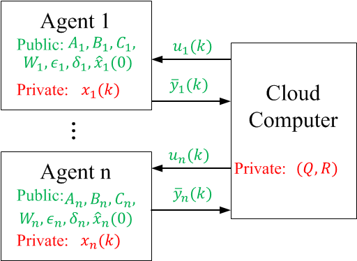
Figure 1: Summary of information available over network.

III-D Reformulation of Problem 1

Having specified exactly the sense in which privacy is implemented in Problem 1, we now give an equivalent statement of Problem 1 as an LQG control problem [3].

Problem 2

Minimize

$$J(x,u)=\lim_{K_{f}\to\infty}\frac{1}{K_{f}}\left[\sum_{k=1}^{K_{f}}x(k)^{T}Qx(k)+u(k)^{T}Ru(k)\right]$$ (15)

over all $u$ with $u(k)\in\mathbb{R}^{m}$, subject to the dynamics and output equations

$$x(k+1) =Ax(k)+Bu(k)+w(k)$$ (16)

$$y(k) =Cx(k)+v(k),$$ (17)

where $C=\textnormal{diag}(C_{1},\ldots,C_{N})$ and where $\hat{x}(0):=\mathbb{E}[x(0)]$ is known and each agent has specified its privacy parameters $(\epsilon_{i},\delta_{i})$. $\blacklozenge$

IV Results: Private LQG Control

In this section we solve Problem 2, with the understanding that this solution also solves Problem 1. Problem 2 takes the form of a Linear Quadratic Gaussian (LQG) problem, which is well-studied in the control literature [3, 2], We first solve Problem 2 using established techniques and then quantify the effects of privacy upon the system. Below, we use the notation $\lambda_{i}(\cdot)$ to denote the $i^{th}$ largest eigenvalue of a matrix and the notation $s_{i}(\cdot)$ to denote the $i^{th}$ largest singular value of a matrix.

IV-A Solving Problem 2

Due to the process noise and privacy noise in Problem 2, the controllers we develop cannot rely on the exact value of $x(k)$. Instead, the controllers used rely on its expected value given all past inputs and outputs, denoted

$$\hat{x}(k):=\mathbb{E}[x(k)\mid u(0),\ldots,u(k-1),y(0),\ldots,y(k-1)].$$ (18)

Problem 2 is an infinite-horizon discrete-time LQG problem, and it is known [4, Section 5.2] that the optimal controller for such problems relies on $\hat{x}(k)$ in the form

$$u^{*}(k)=L\hat{x}(k).$$ (19)

Here,

$$L=-(R+B^{T}KB)^{-1}B^{T}KA,$$ (20)

and $K$ is the unique positive semidefinite solution to the discrete algebraic Riccati equation

$$K=A^{T}KA-A^{T}KB(R+B^{T}KB)^{-1}B^{T}KA+Q.$$ (21)

Computing the state estimate $\hat{x}(k)$ can be done for infinite time horizons using the time-invariant Kalman filter [4, Section 5.2]

$$\hat{x}(k+1)+\overline{\Sigma}C^{T}V^{-1}\big{(}\bar{y}(k+1)-C(A+BL)\hat{x}(k)\big{)},$$ (22)

where $\overline{\Sigma}$ is given by

$$\overline{\Sigma}=\Sigma-\Sigma C^{T}(C\Sigma C^{T}+V)^{-1}C\Sigma,$$ (23)

and where $\Sigma$ is the unique positive semidefinite solution to the discrete algebraic Riccati equation

$$\Sigma=A\Sigma A^{T}-A\Sigma C^{T}(C\Sigma C^{T}+V)^{-1}C\Sigma A^{T}+W.$$ (24)

As discussed in Section III-B, the cloud is responsible for generating control values for each agent at each point in time. Therefore, the cloud will run the Kalman filter in Equation (22) and will likewise generate control values using Equation (19). Thus the flow of information in the network first has agent $i$ send $\bar{y}_{i}(k)$ to the cloud at time $k$, and then has the cloud form $\bar{y}(k)=\big{(}\bar{y}_{1}(k)^{T},\ldots,\bar{y}_{N}(k)^{T}\big{)}^{T}$ and use it to estimate $\hat{x}(k+1)$. Next, the cloud computes $u^{*}(k)=L\hat{x}(k)$, and finally the cloud sends $u^{*}_{i}(k)$ to agent $i$. We emphasize that the cloud only sends $u^{*}_{i}(k)$ to agent $i$ and, because sharing this control value can threaten its privacy, agent $i$ does not share this control value with any other agent.

With respect to implementation, the matrices $K$, $L$, $\overline{\Sigma}$, and $\Sigma$ can all be computed offline by the cloud a single time before the network begins solving Problem 1. Then these matrices can be used repeatedly in generating control values to send to the agents, substantially reducing the cloud’s computational burden at runtime and allowing it to quickly generate state estimates and control values. With this in mind, we now state the full solution to Problem 1 below in Algorithm 1.

Data: Public information $A_{i}$, $B_{i}$, $C_{i}$, $\epsilon_{i}$, $\delta_{i}$, $\hat{x}_{i}(0)$

1 Initialize the cloud with all public information

2 For all $i$, initialize agent $i$ with $A_{i}$, $B_{i}$, $C_{i}$. Agent $i$ chooses $(\epsilon_{i},\delta_{i})$ and knows its exact initial state $x_{i}(0)$ but does not share it.

3 In the cloud, precompute $L$ using Equation (20) and $\overline{\Sigma}$ according to Equation (23)

4 for $k=0,1,2,\ldots$ do

5       for $i=1,\ldots,N$ do

6             Agent $i$ generates $v_{i}(k)\sim\mathcal{N}(0,\sigma_{i}I_{n_{i}})$

7             Agent $i$ sends the cloud the private output $\bar{y}_{i}(k):=C_{i}x_{i}(k)+v_{i}(k)$

8      In the cloud, compute $\hat{x}(k)$ with Equation (22)

9       In the cloud, compute $u^{*}(k)=L\hat{x}(k)$ and send $u^{*}_{i}(k)$ to agent $i$

10       for $i=1,\ldots,N$ do

11             Agent $i$ updates its state via $x_{i}(k+1)=A_{i}x_{i}(k)+B_{i}u^{*}_{i}(k)+w_{i}(k)$

12      

Algorithm 1 Differentially Private LQG (Solution to Problem 1)

IV-B Quantifying the Effects of Privacy

Algorithm 1 solves Problem 2, though it is intuitively clear that adding noise for the sake of privacy will diminish the ability of the cloud to compute optimal control values. Indeed, the purpose of differential privacy in this problem is to protect an agent’s state value from the cloud (and any eavesdroppers). Here, we quantify the trade-off between privacy and the ability of the cloud to accurately estimate the agents’ state values.

The cloud both implements a Kalman filter and computes the controller $u^{*}(k)$, though noise added for privacy only affects the Kalman filter. Note that the network-level optimal controller defined in Equation (19) takes the form $u^{*}(k)=L\hat{x}(k)$, while the optimal controller with no privacy noise (i.e., $v(k)\equiv 0$ for all $k$) would take the same form with the expectation carried out only over the process noise. Similarly, in the deterministic case of $v(k)\equiv 0$ and $w(k)\equiv 0$ for all $k$, the optimal controller is $u^{*}(k)=Lx(k)$. The optimal controller in all three cases is linear and defined by $L$, and the only difference between these controllers comes from changes in the estimate of $x(k)$ or in using $x(k)$ exactly. This is an example of the so-called “certainty equivalence principle” [4], and it demonstrates that the controller in Algorithm 1 is entirely unaware of the presence or absence of noise. Instead, the effects of noise in the system are compensated for by the Kalman filter defined in Equation (22), and we therefore examine the impact of privacy noise upon the Kalman filter that informs the controller used in Algorithm 1. Related work in [18] specifies procedures for designing differentially private Kalman filters, though here we use a Kalman filter to process private data and quantify the effects of privacy upon the filter itself. To the best of our knowledge this is the first study to do so.

One natural way to study this trade-off is through bounding the information content in the Kalman filter as a function of the privacy noise, as differential privacy explicitly seeks to mask sensitive information by corrupting it with noise. In our case, we consider the differential entropy of $\hat{x}$ as a proxy for the information content of the signal [6]. Shannon entropy has been used to quantify the effects of differential privacy in other settings, including in distributed linear control systems where database-type differential privacy is applied [22] Though differential entropy does not have the same axiomatic foundation as Shannon entropy, it is useful for Gaussian distributions because it bounds the extent of the sublevel sets of $\mathcal{R}^{-1}$ where $\mathcal{R}(y)=1-2\mathcal{Q}(y)$, i.e., the volume of covariance ellipsoids. We can therefore quantify the effects of differentially private masking upon the cloud by studying how privacy noise changes the $\log\det({\Sigma})$, which is within a constant factor of the differential entropy of $\hat{x}$. The analysis we present differs from previous work because we apply trajectory-level differential privacy and quantify the resulting differential entropy in the Kalman filter. Toward presenting this result, we have the following lemma concerning the determinants of matrices related by a matrix inequality.

Lemma 2

Let $P\succeq 0$ and $Q\succeq 0$ satisfy $P\succeq Q$. Then $\textnormal{det}(P)\geq\textnormal{det}(Q)$ and $\log\det(P)\geq\log\det(Q)$.

Proof: This follows from the monotonicity of $\log$ and the fact that $\lambda_{i}(X)\geq\lambda_{i}(Y)$ [16, Theorem 16.F.1] whenever $X\succeq Y$. $\blacksquare$

Next we have the following lemma that relates the determinant of a matrix to its trace.

Lemma 3

Let $M\in\mathbb{R}^{n\times n}$ be a positive semi-definite matrix. Then

$$\det(M)\leq\left(\frac{\textnormal{tr}(M)}{n}\right)^{n}.$$

Proof: The positive semi-definiteness of $M$ implies that all of its eigenvalues are non-negative. The result then follows by applying the AM-GM inequality to the eigenvalues of $M$. $\blacksquare$

Finally, we have the following lemma which gives a matrix upper bound on solutions to a discrete algebraic Riccati equation.

Lemma 4

Suppose $\Sigma$ is the unique positive semi-definite solution to the equation

$$\Sigma=A(\Sigma-\Sigma C^{T}(C\Sigma C^{T}+V)^{-1}C\Sigma)A^{T}+W,$$ (25)

and define

$$\gamma_{i}=\frac{\sigma_{i}^{2}W_{ii}}{\sigma_{i}^{2}+C_{ii}^{2}W_{ii}},$$ (26)

with $\Gamma=\textnormal{diag}(\gamma_{1},\ldots,\gamma_{n})$. Then

$$\lambda_{1}(\Sigma)\geq s_{n}^{2}(A)\lambda_{1}(\Gamma)+\lambda_{n}(W)=:\eta.$$ (27)

Furthermore, if

$$s_{1}^{2}(A)<1+\big{(}s_{n}^{2}(A)\lambda_{1}(\Gamma)+\lambda_{n}(W)\big{)}\cdot\min_{i\in[n]}\frac{C_{ii}^{2}}{\sigma_{i}^{2}},$$ (28)

then

$$\Sigma\preceq\frac{\lambda_{1}(W)}{1+\eta\lambda_{n}(C^{T}V^{-1}C)-s_{1}^{2}(A)}AA^{T}+W.$$ (29)

Proof: This follows from Theorem 2 in [14]. $\blacksquare$

We now present our main results on bounding the log-determinant of the steady-state Kalman filter error covariance in the private LQG problem. In particular, we study the log-determinant of the a priori error covariance, $\Sigma$, because $\Sigma$ measures the error in the cloud’s predictions about the state of the system. Bounding the log-determinant of $\Sigma$ therefore bounds the entropy seen at the cloud when making predictions about the state of the network in the presence of noise added for privacy.

Theorem 1

Let $\Sigma$ denote the steady-state a priori error covariance in the cloud’s Kalman filter in Algorithm 1. If all hypotheses of Lemma 4 hold, $C_{i}$ is square and diagonal for all $i$, and Assumption 1 holds, then

$$\log\det\Sigma<\left(\frac{\lambda_{1}(W)}{1+\eta\lambda_{n}(C^{T}V^{-1}C)-s_{1}^{2}(A)}\right)\sum_{i=1}^{n}s_{i}^{2}(A)+\textnormal{tr}(W),$$ (30)

with $\eta$ defined as in Lemma 4, and where the term

$$\eta\lambda_{n}(C^{T}V^{-1}C)=s_{n}^{2}(A)\cdot\max_{i\in[n]}\frac{\sigma_{i}^{2}W_{ii}}{\sigma_{i}^{2}+C_{ii}^{2}W_{ii}}\cdot\min_{i\in[n]}\frac{C_{ii}^{2}}{\sigma_{i}^{2}}+\lambda_{n}(W)\cdot\min_{i\in[n]}\frac{C_{ii}^{2}}{\sigma_{i}^{2}}$$ (31)

is the only one affected by privacy.

Proof: With the assumption that each $C_{i}$ is square and diagonal, we see that

$$C^{T}V^{-1}C=\textnormal{diag}\left(\frac{C_{11}^{2}}{\sigma_{1}^{2}},\ldots,\frac{C_{nn}^{2}}{\sigma_{n}^{2}}\right),$$ (32)

which gives

$$\lambda_{n}\Big{(}C^{T}V^{-1}C\Big{)}=\min_{1\leq i\leq n}\frac{C_{ii}^{2}}{\sigma_{i}^{2}},$$ (33)

and the form of $\eta\lambda_{n}(C^{T}V^{-1}C)$ follows.

Lemma 4 then gives

$$\Sigma\preceq\frac{\lambda_{1}(W)}{1+\eta\lambda_{n}(C^{T}V^{-1}C)-s_{1}^{2}(A)}AA^{T}+W,$$ (34)

where applying Lemma 2 gives

$$\det\Sigma\leq\det\bigg{[}\frac{\lambda_{1}(W)}{1+\eta\lambda_{n}(C^{T}V^{-1}C)-s_{1}^{2}(A)}AA^{T}+W\bigg{]}.$$ (35)

The argument of the determinant on the right-hand side is a positive-definite matrix, and applying Lemma 3 therefore gives

$$\det\Sigma\leq\left(\frac{\textnormal{tr}\left(\frac{\lambda_{1}(W)}{1+\eta\lambda_{n}(C^{T}V^{-1}C)-s_{1}^{2}(A)}AA^{T}+W\right)}{n}\right)^{n}.$$ (36)

Taking the natural logarithm of both sides, we find that

$$\log\det\Sigma \leq\log\left(\frac{\textnormal{tr}\left(\frac{\lambda_{1}(W)}{1+\eta\lambda_{n}(C^{T}V^{-1}C)-s_{1}^{2}(A)}AA^{T}+W\right)}{n}\right)^{n}$$ (37)

$$=n\log\left(\frac{\textnormal{tr}\left(\frac{\lambda_{1}(W)}{1+\eta\lambda_{n}(C^{T}V^{-1}C)-s_{1}^{2}(A)}AA^{T}+W\right)}{n}\right)$$ (38)

$$<n\left(\frac{\textnormal{tr}\left(\frac{\lambda_{1}(W)}{1+\eta\lambda_{n}(C^{T}V^{-1}C)-s_{1}^{2}(A)}AA^{T}+W\right)}{n}\right),$$ (39)

which follows from the fact that $\log x<x$ for all $x>0$. Continuing, we find that

$$\log\det\Sigma <\textnormal{tr}\left(\frac{\lambda_{1}(W)}{1+\eta\lambda_{n}(C^{T}V^{-1}C)-s_{1}^{2}(A)}AA^{T}+W\right)$$ (40)

$$=\frac{\lambda_{1}(W)}{1+\eta\lambda_{n}(C^{T}V^{-1}C)-s_{1}^{2}(A)}\textnormal{tr}(AA^{T})+\textnormal{tr}(W),$$ (41)

which follows from the linearity of the trace operator. The theorem follows by expanding the trace of $AA^{T}$ in terms of the singular values of $A$. $\blacksquare$

Remark 1

To interpret Theorem 1, we consider the case in which $C_{i}=I_{n_{i}}$ for all $i$, indicating that the cloud simply requests each agent’s state at each point in time, in which $W_{i}=\omega I_{n_{i}}$, indicating that each agent has identical noise covariance for its process noise, and in which $\epsilon_{i}=\epsilon$ and $\delta_{i}=\delta$ for all $i$ and some $\epsilon>0$ and $\delta\in(0,1/2)$. In this case, $\sigma_{i}=\sigma$ for all $i$ and we find

$$\eta\lambda_{n}(C^{T}V^{-1}C)=s_{n}^{2}(A)\frac{\omega}{\sigma^{2}+\omega}+\frac{\omega}{\sigma^{2}}.$$ (42)

If the other terms in the denominator can be neglected in Theorem 1, then one finds that

$$\log\det\Sigma\lessapprox\left(\frac{s_{n}^{2}(A)}{\sigma^{2}+\omega}+\frac{1}{\sigma^{2}}\right)^{-1}\sum_{i=1}^{n}s_{i}^{2}(A)+n\omega,$$ (43)

indicating that, in this case, a linear change in the variance of privacy noise $\sigma$ incurs a roughly quadratic increase in entropy. $\lozenge$

V Case Study

In this section, we use a two-agent example to illustrate the use of Algorithm 1. Consider a two-agent system with $x_{1}(k),x_{2}(k)\in\mathbb{R}^{2}$ for all $k$, and where each agent has identical dynamics and process noise covariance matrices

$$A_{i}=\begin{bmatrix}1&0.1\\ 0&1\end{bmatrix},B_{i}=\begin{bmatrix}0\\ 1\end{bmatrix},W_{i}=\begin{bmatrix}1&0.5\\ 0.5&1.0\end{bmatrix}.$$ (44)

In this case, we can interpret the first coordinate of each agent’s position and the second coordinate as its velocity. Consider the case in which the two agents select different privacy parameters, namely,

$$(\epsilon_{1},\delta_{1})=(0.1,0.01)\textnormal{ and }(\epsilon_{2},\delta_{2})=(1,0.5),$$ (45)

giving $\sigma_{1}=23.48$ and $\sigma_{2}=0.71$.

These parameters mean that Agent 1 has chosen to be much more private than Agent 2. Algorithm 1 was simulated for this problem for $200$ timesteps, and the results of this simulation are shown in Figure 2. For these simulations, the $Q,R$ matrices were randomly chosen positive definite matrices for which the off-diagonal elements were non-zero, meaning that the cost $J$ is not separable over agents. Note that the estimated trajectory of Agent 1, which is the optimal estimate (in the least squares sense) for both the aggregator and an adversary, shows substantial temporal variation and is in general very different from the true trajectory. However, even with the degraded information reported to the aggregator, the state of Agent 1 is still controlled closely to its desired value. And, although the aggregator substantially overestimates the incurred cost due to the injected privacy noise, the true incurred average cost over time remains bounded here.

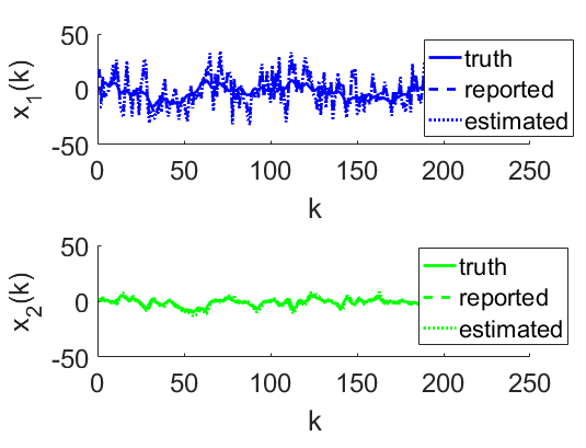
(a)

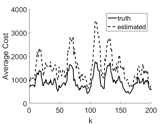
(b)

Figure 2: Examples of applying the DPLQG to a two agent network. (a) Agent position trajectories (b) Moving average cost.

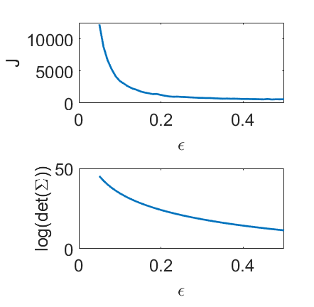
Figure 3: Effect of privacy parameter $\epsilon$ on cost and estimation accuracy.

The effect of privacy parameters is further illustrated in Figure 3. In this case, we consider a network with 4 agents with dynamics matrices as stated in Equation (44), and fix the parameters $\epsilon_{i}=\epsilon$ and $\delta_{i}=0.25$ for all agents. Figure 3 shows the effect on the cost $J$ (estimated from 2500 time steps) and the state estimate uncertainty $\log\det(\Sigma)$ as we vary the parameter $\epsilon$. These plots show that each quantity varies monotonically and smoothly with $\epsilon$, demonstrating that changing the overall privacy level in the system indeed results in predictable changes in the behavior of the system, as predicted by Theorem 1.

VI Conclusions

In this paper, we have studied the problem of distributed linear quadratic optimal control with agent-specified differential privacy requirements. To our knowledge, this is the first paper to consider the effects of trajectory-level differential privacy in feedback. Here, we have related this problem to the well-studied LQG problem and have shown how to bound the uncertainty in the network-level joint state estimate in terms of the privacy parameters specified by the individual agents. Future work includes considering more general classes of control and estimation models and nested and sequential feedback loops.

References

- [1] B. Anderson and J. Moore. Optimal Control: Linear Quadratic Methods. Prentice-Hall, Inc., Upper Saddle River, NJ, USA, 1990.
- [2] Karl Johan Astrom. Introduction to stochastic control theory, volume 70 of Mathematics in science and engineering. Academic Press, 1970.
- [3] M. Athans. The role and use of the stochastic linear-quadratic-gaussian problem in control system design. IEEE Transactions on Automatic Control, 16(6):529–552, Dec 1971.
- [4] Dimitri P Bertsekas. Dynamic programming and optimal control, volume 1. Athena Scientific Belmont, MA, 3 edition, 2005.
- [5] Stephen Boyd and Lieven Vandenberghe. Convex Optimization. Cambridge University Press, New York, NY, USA, 2004.
- [6] Thomas M Cover and Joy A Thomas. Elements of information theory. John Wiley & Sons, 2012.
- [7] Cynthia Dwork, Frank McSherry, Kobbi Nissim, and Adam Smith. Calibrating noise to sensitivity in private data analysis. In Theory of Cryptography Conference, pages 265–284. Springer, 2006.
- [8] Cynthia Dwork, Aaron Roth, et al. The algorithmic foundations of differential privacy. Foundations and Trends® in Theoretical Computer Science, 9(3–4):211–407, 2014.
- [9] A Greenberg. Apple’s’ differential privacy is about collecting your data—but not your data. Wired, June, 2016.
- [10] M. T. Hale and M. Egerstedt. Cloud-based optimization: A quasi-decentralized approach to multi-agent coordination. In 53rd IEEE Conference on Decision and Control, pages 6635–6640, Dec 2014.
- [11] Matthew Hale and Magnus Egerstedt. Cloud-enabled differentially private multi-agent optimization with constraints. arXiv preprint arXiv:1507.04371, 2015.
- [12] Roger A. Horn and Charles R. Johnson, editors. Matrix Analysis. Cambridge University Press, New York, NY, USA, 1986.
- [13] Shiva Prasad Kasiviswanathan and Adam Smith. On the semantics of differential privacy: A bayesian formulation. arXiv preprint arXiv:0803.3946, 2008.
- [14] C. Lee. Upper matrix bound of the solution for the discrete riccati equation. IEEE Trans. on Automatic Control, 42(6):840–842, 1997.
- [15] A. Machanavajjhala, D. Kifer, J. Abowd, J. Gehrke, and L. Vilhuber. Privacy: Theory meets practice on the map. In IEEE 24th International Conference on Data Engineering, pages 277–286, 2008.
- [16] Albert W Marshall, Ingram Olkin, and Barry C Arnold. Inequalities: theory of majorization and its applications. Springer, New York, NY, USA, 2nd edition, 2009.
- [17] J. Le Ny and M. Mohammady. Differentially private mimo filtering for event streams and spatio-temporal monitoring. In 53rd IEEE Conference on Decision and Control, pages 2148–2153, Dec 2014.
- [18] J. Le Ny and G. J. Pappas. Differentially private filtering. IEEE Transactions on Automatic Control, 59(2):341–354, 2014.
- [19] U.S. Department of Energy. Department of energy data access and privacy issues related to smart grid technologies. Technical report, U.S. DoE, 2010.
- [20] Ozgur Koray Sahingoz. Networking models in flying ad-hoc networks (fanets): Concepts and challenges. Journal of Intelligent & Robotic Systems, 74(1-2):513, 2014.
- [21] E. Sontag. Mathematical control theory: deterministic finite dimensional systems, volume 6. Springer Science & Business Media, 2013.
- [22] Y. Wang, Z. Huang, S. Mitra, and G. E. Dullerud. Entropy-minimizing mechanism for differential privacy of discrete-time linear feedback systems. In 53rd IEEE Conference on Decision and Control, pages 2130–2135, Dec 2014.
- [23] H. Yang, H. Luo, F. Ye, S. Lu, and L. Zhang. Security in mobile ad hoc networks: challenges and solutions. IEEE wireless communications, 11(1):38–47, 2004.
- [24] P. Zhang, C. Lin, Y. Jiang, Y. Fan, and X. Shen. A lightweight encryption scheme for network-coded mobile ad hoc networks. IEEE Transactions on Parallel and Distributed Systems, 25(9):2211–2221, 2014.