A Brief Introduction to Machine Learning for Engineers

Abstract

This monograph aims at providing an introduction to key concepts, algorithms, and theoretical results in machine learning. The treatment concentrates on probabilistic models for supervised and unsupervised learning problems. It introduces fundamental concepts and algorithms by building on first principles, while also exposing the reader to more advanced topics with extensive pointers to the literature, within a unified notation and mathematical framework. The material is organized according to clearly defined categories, such as discriminative and generative models, frequentist and Bayesian approaches, exact and approximate inference, as well as directed and undirected models. This monograph is meant as an entry point for researchers with an engineering background in probability and linear algebra.

MLEE.bib Osvaldo Simeone
Department of Informatics
King’s College London
osvaldo.simeone@kcl.ac.uk

1]Department of Informatics, King’s College London; osvaldo.simeone@kcl.ac.uk

Notation

$\bullet$ Random variables or random vectors – both abbreviated as rvs – are represented using roman typeface, while their values and realizations are indicated by the corresponding standard font. For instance, the equality $\mathrm{x}=x$ indicates that rv $\mathrm{x}$ takes value $x$.
$\bullet$ Matrices are indicated using uppercase fonts, with roman typeface used for random matrices.
$\bullet$ Vectors will be taken to be in column form.
$\bullet$ $X^{T}$ and $X^{\dagger}$ are the transpose and the pseudoinverse of matrix $X$, respectively.
$\bullet$ The distribution of a rv $\mathrm{x}$, either probability mass function (pmf) for a discrete rv or probability density function (pdf) for continuous rvs, is denoted as $p_{\mathrm{x}}$, $p_{\mathrm{x}}(x)$, or $p(x)$.
$\bullet$ The notation $\mathrm{x}\sim p_{\mathrm{x}}$ indicates that rv $\mathrm{x}$ is distributed according to $p_{\mathrm{x}}$.
$\bullet$ For jointly distributed rvs $(\mathrm{x,y})\sim p_{\mathrm{xy}}$, the conditional distribution of $\mathrm{x}$ given the observation $\mathrm{y}=y$ is indicated as $p_{\mathrm{x|}\mathrm{y}=y}$, $p_{\mathrm{x|y}}(x|y)$ or $p(x|y)$.
$\bullet$ The notation $\mathrm{x|y}=y\sim p_{\mathrm{x|y}=y}$ indicates that rv $\mathrm{x}$ is drawn according to the conditional distribution $p_{\mathrm{x|y}=y}$.
$\bullet$ The notation $\textrm{E}_{\mathrm{x}\sim p_{\mathrm{x}}}[\cdot]$ indicates the expectation of the argument with respect to the distribution of the rv $\mathrm{x}\sim p_{\mathrm{x}}$. Accordingly, we will also write $\textrm{E}_{\mathrm{x}\sim p_{\mathrm{x|y}}}[\cdot|y]$ for the conditional expectation with respect to the distribution $p_{\mathrm{x|}\mathrm{y}=y}$. When clear from the context, the distribution over which the expectation is computed may be omitted.
$\bullet$ The notation $\textrm{Pr}_{\mathrm{x}\sim p_{\mathrm{x}}}[\cdot]$ indicates the probability of the argument event with respect to the distribution of the rv $\mathrm{x}\sim p_{\mathrm{x}}$. When clear from the context, the subscript is dropped.
$\bullet$ The notation $\log$ represents the logarithm in base two, while $\ln$ represents the natural logarithm.
$\bullet$ $\mathrm{x}\sim\mathcal{N}(\mu,\Sigma)$ indicates that random vector $\mathrm{x}$ is distributed according to a multivariate Gaussian pdf with mean vector $\mu$ and covariance matrix $\Sigma$. The multivariate Gaussian pdf is denoted as $\mathcal{N}(x|\mu,\Sigma)$ as a function of $x$.
$\bullet$ $\mathrm{x}\sim\mathcal{U}(a,b)$ indicates that rv $\mathrm{x}$ is distributed according to a uniform distribution in the interval $[a,b]$. The corresponding uniform pdf is denoted as $\mathcal{U}(x|a,b)$.
$\bullet$ $\delta(x)$ denotes the Dirac delta function or the Kronecker delta function, as clear from the context.
$\bullet$ $||a||^{2}=\sum_{i=1}^{N}a_{i}^{2}$ is the quadratic, or $l_{2}$, norm of a vector $a=[a_{1},...,a_{N}]^{T}$. We similarly define the $l_{1}$ norm as $||a||_{1}=\sum_{i=1}^{N}|a_{i}|$, and the $l_{0}$ pseudo-norm $||a||_{0}$ as the number of non-zero entries of vector $a$.
$\bullet$ $I$ denotes the identity matrix, whose dimensions will be clear from the context. Similarly, $1$ represents a vector of all ones.
$\bullet$ $\mathbb{R}$ is the set of real numbers; $\mathbb{R}^{+}$ the set of non-negative real numbers; $\mathbb{R}^{-}$ the set of non-positive real numbers; and $\mathbb{R}^{N}$ is the set of all vectors of $N$ real numbers.
$\bullet$ $1\left(\cdot\right)$ is the indicator function: $1\left(x\right)=1$ if $x$ is true, and $1\left(x\right)=0$ otherwise.
$\bullet$ $|\mathcal{S}|$ represents the cardinality of a set $\mathcal{S}$.
$\bullet$ $x_{\mathcal{S}}$ represents a set of rvs $x_{k}$ indexed by the integers $k\in\mathcal{S}$.

Acronyms

AI: Artificial Intelligence
AMP: Approximate Message Passing
BN: Bayesian Network
DAG: Directed Acyclic Graph
ELBO: Evidence Lower BOund
EM: Expectation Maximization
ERM: Empirical Risk Minimization
GAN: Generative Adversarial Network
GLM: Generalized Linear Model
HMM: Hidden Markov Model
i.i.d.: independent identically distributed
KL: Kullback-Leibler
LASSO: Least Absolute Shrinkage and Selection Operator
LBP: Loopy Belief Propagation
LL: Log-Likelihood
LLR: Log-Likelihood Ratio
LS: Least Squares
MC: Monte Carlo
MCMC: Markov Chain Monte Carlo
MDL: Minimum Description Length
MFVI: Mean Field Variational Inference
ML: Maximum Likelihood
MRF: Markov Random Field
NLL: Negative Log-Likelihood
PAC: Probably Approximately Correct
pdf: probability density function
pmf: probability mass function
PCA: Principal Component Analysis
PPCA: Probabilistic Principal Component Analysis
QDA: Quadratic Discriminant Analysis
RBM: Restricted Boltzmann Machine
SGD: Stochastic Gradient Descent
SVM: Support Vector Machine
rv: random variable or random vector (depending on the context)
s.t.: subject to
VAE: Variational AutoEncoder
VC: Vapnik–Chervonenkis
VI: Variational Inference

Part I Basics

Chapter 1 Introduction

Having taught courses on machine learning, I am often asked by colleagues and students with a background in engineering to suggest “the best place to start” to get into this subject. I typically respond with a list of books – for a general, but slightly outdated introduction, read this book; for a detailed survey of methods based on probabilistic models, check this other reference; to learn about statistical learning, I found this text useful; and so on. This answer strikes me, and most likely also my interlocutors, as quite unsatisfactory. This is especially so since the size of many of these books may be discouraging for busy professionals and students working on other projects. This monograph is an attempt to offer a basic and compact reference that describes key ideas and principles in simple terms and within a unified treatment, encompassing also more recent developments and pointers to the literature for further study.

1.1 What is Machine Learning?

A useful way to introduce the machine learning methodology is by means of a comparison with the conventional engineering design flow. This starts with a in-depth analysis of the problem domain, which culminates with the definition of a mathematical model. The mathematical model is meant to capture the key features of the problem under study, and is typically the result of the work of a number of experts. The mathematical model is finally leveraged to derive hand-crafted solutions to the problem.

For instance, consider the problem of defining a chemical process to produce a given molecule. The conventional flow requires chemists to leverage their knowledge of models that predict the outcome of individual chemical reactions, in order to craft a sequence of suitable steps that synthesize the desired molecule. Another example is the design of speech translation or image/ video compression algorithms. Both of these tasks involve the definition of models and algorithms by teams of experts, such as linguists, psychologists, and signal processing practitioners, not infrequently during the course of long standardization meetings.

The engineering design flow outlined above may be too costly and inefficient for problems in which faster or less expensive solutions are desirable. The machine learning alternative is to collect large data sets, e.g., of labelled speech, images or videos, and to use this information to train general-purpose learning machines to carry out the desired task. While the standard engineering flow relies on domain knowledge and on design optimized for the problem at hand, machine learning lets large amounts of data dictate algorithms and solutions. To this end, rather than requiring a precise model of the set-up under study, machine learning requires the specification of an objective, of a model to be trained, and of an optimization technique.

Returning to the first example above, a machine learning approach would proceed by training a general-purpose machine to predict the outcome of known chemical reactions based on a large data set, and by then using the trained algorithm to explore ways to produce more complex molecules. In a similar manner, large data sets of images or videos would be used to train a general-purpose algorithm with the aim of obtaining compressed representations from which the original input can be recovered with some distortion.

1.2 When to Use Machine Learning?

Based on the discussion above, machine learning can offer an efficient alternative to the conventional engineering flow when development cost and time are the main concerns, or when the problem appears to be too complex to be studied in its full generality. On the flip side, the approach has the key disadvantages of providing generally suboptimal performance, or hindering interpretability of the solution, and to apply only to a limited set of problems.

In order to identify tasks for which machine learning methods may be useful, reference [mitchell17] suggests the following criteria:

1. the task involves a function that maps well-defined inputs to well-defined outputs;

2. large data sets exist or can be created containing input-output pairs;

3. the task provides clear feedback with clearly definable goals and metrics;

4. the task does not involve long chains of logic or reasoning that depend on diverse background knowledge or common sense;

5. the task does not require detailed explanations for how the decision was made;

6. the task has a tolerance for error and no need for provably correct or optimal solutions;

7. the phenomenon or function being learned should not change rapidly over time; and

8. no specialized dexterity, physical skills, or mobility is required.

These criteria are useful guidelines for the decision of whether machine learning methods are suitable for a given task of interest. They also offer a convenient demarcation line between machine learning as is intended today, with its focus on training and computational statistics tools, and more general notions of Artificial Intelligence (AI) based on knowledge and common sense [Levesque17] (see [norvig2009] for an overview on AI research).

1.2.1 Learning Tasks

We can distinguish among three different main types of machine learning problems, which are briefly introduced below. The discussion reflects the focus of this monograph on parametric probabilistic models, as further elaborated on in the next section.

1. Supervised learning: We have $N$ labelled training examples $\text{$\mathcal{D}$=}\{(x_{n},t_{n})\}_{n=1}^{N},$ where $x_{n}$ represents a covariate, or explanatory variable, while $t_{n}$ is the corresponding label, or response. For instance, variable $x_{n}$ may represent the text of an email, while the label $t_{n}$ may be a binary variable indicating whether the email is spam or not. The goal of supervised learning is to predict the value of the label $t$ for an input $x$ that is not in the training set. In other words, supervised learning aims at generalizing the observations in the data set $\mathcal{D}$ to new inputs. For example, an algorithm trained on a set of emails should be able to classify a new email not present in the data set $\mathcal{D}$.

We can generally distinguish between classification problems, in which the label $t$ is discrete, as in the example above, and regression problems, in which variable $t$ is continuous. An example of a regression task is the prediction of tomorrow’s temperature $t$ based on today’s meteorological observations $x$.

An effective way to learn a predictor is to identify from the data set $\mathcal{D}$ a predictive distribution $p(t|x)$ from a set of parametrized distributions. The conditional distribution $p(t|x)$ defines a profile of beliefs over all possible of the label $t$ given the input $x$. For instance, for temperature prediction, one could learn mean and variance of a Gaussian distribution $p(t|x)$ as a function of the input $x$. As a special case, the output of a supervised learning algorithm may be in the form of a deterministic predictive function $t=\hat{t}(x)$.

2. Unsupervised learning: Suppose now that we have an unlabelled set of training examples $\text{$\mathcal{D}$=}\{x_{n}\}_{n=1}^{N}.$ Less well defined than supervised learning, unsupervised learning generally refers to the task of learning properties of the mechanism that generates this data set. Specific tasks and applications include clustering, which is the problem of grouping similar examples $x_{n}$; dimensionality reduction, feature extraction, and representation learning, all related to the problem of representing the data in a smaller or more convenient space; and generative modelling, which is the problem of learning a generating mechanism to produce artificial examples that are similar to available data in the data set $\mathcal{D}$.

As a generalization of both supervised and unsupervised learning, semi-supervised learning refers to scenarios in which not all examples are labelled, with the unlabelled examples providing information about the distribution of the covariates $x$.

3. Reinforcement learning: Reinforcement learning refers to the problem of inferring optimal sequential decisions based on rewards or punishments received as a result of previous actions. Under supervised learning, the “label” $t$ refers to an action to be taken when the learner is in an informational state about the environment given by a variable $x$. Upon taking an action $t$ in a state $x$, the learner is provided with feedback on the immediate reward accrued via this decision, and the environment moves on to a different state. As an example, an agent can be trained to navigate a given environment in the presence of obstacles by penalizing decisions that result in collisions.

Reinforcement learning is hence neither supervised, since the learner is not provided with the optimal actions $t$ to select in a given state $x$; nor is it fully unsupervised, given the availability of feedback on the quality of the chosen action. Reinforcement learning is also distinguished from supervised and unsupervised learning due to the influence of previous actions on future states and rewards.

This monograph focuses on supervised and unsupervised learning. These general tasks can be further classified along the following dimensions.

$\bullet$ Passive vs. active learning: A passive learner is given the training examples, while an active learner can affect the choice of training examples on the basis of prior observations.

$\bullet$ Offline vs. online learning: Offline learning operates over a batch of training samples, while online learning processes samples in a streaming fashion. Note that reinforcement learning operates inherently in an online manner, while supervised and unsupervised learning can be carried out by following either offline or online formulations.

This monograph considers only passive and offline learning.

1.3 Goals and Outline

This monograph aims at providing an introduction to key concepts, algorithms, and theoretical results in machine learning. The treatment concentrates on probabilistic models for supervised and unsupervised learning problems. It introduces fundamental concepts and algorithms by building on first principles, while also exposing the reader to more advanced topics with extensive pointers to the literature, within a unified notation and mathematical framework. Unlike other texts that are focused on one particular aspect of the field, an effort has been made here to provide a broad but concise overview in which the main ideas and techniques are systematically presented. Specifically, the material is organized according to clearly defined categories, such as discriminative and generative models, frequentist and Bayesian approaches, exact and approximate inference, as well as directed and undirected models. This monograph is meant as an entry point for researchers with a background in probability and linear algebra. A prior exposure to information theory is useful but not required.

Detailed discussions are provided on basic concepts and ideas, including overfitting and generalization, Maximum Likelihood and regularization, and Bayesian inference. The text also endeavors to provide intuitive explanations and pointers to advanced topics and research directions. Sections and subsections containing more advanced material that may be skipped at a first reading are marked with a star ($*$).

The reader will find here neither discussions on computing platform or programming frameworks, such as map-reduce, nor details on specific applications involving large data sets. These can be easily found in a vast and growing body of work. Furthermore, rather than providing exhaustive details on the existing myriad solutions in each specific category, techniques have been selected that are useful to illustrate the most salient aspects. Historical notes have also been provided only for a few selected milestone events.

Finally, the monograph attempts to strike a balance between the algorithmic and theoretical viewpoints. In particular, all learning algorithms are introduced on the basis of theoretical arguments, often based on information-theoretic measures. Moreover, a chapter is devoted to statistical learning theory, demonstrating how to set the field of supervised learning on solid theoretical foundations. This chapter is more theoretically involved than the others, and proofs of some key results are included in order to illustrate the theoretical underpinnings of learning. This contrasts with other chapters, in which proofs of the few theoretical results are kept at a minimum in order to focus on the main ideas.

The rest of the monograph is organized into five parts. The first part covers introductory material. Specifically, Chapter 2 introduces the frequentist, Bayesian and Minimum Description Length (MDL) learning frameworks; the discriminative and generative categories of probabilistic models; as well as key concepts such as training loss, generalization, and overfitting – all in the context of a simple linear regression problem. Information-theoretic metrics are also briefly introduced, as well as the advanced topics of interpretation and causality. Chapter 3 then provides an introduction to the exponential family of probabilistic models, to Generalized Linear Models (GLMs), and to energy-based models, emphasizing main properties that will be invoked in later chapters.

The second part concerns supervised learning. Chapter 4 covers linear and non-linear classification methods via discriminative and generative models, including Support Vector Machines (SVMs), kernel methods, logistic regression, multi-layer neural networks and boosting. Chapter 5 is a brief introduction to the statistical learning framework of the Probably Approximately Correct (PAC) theory, covering the Vapnik–Chervonenkis (VC) dimension and the fundamental theorem of PAC learning.

The third part, consisting of a single chapter, introduced unsupervised learning. In particular, in Chapter 6, unsupervised learning models are described by distinguishing among directed models, for which Expectation Maximization (EM) is derived as the iterative maximization of the Evidence Lower BOund (ELBO); undirected models, for which Restricted Boltzmann Machines (RBMs) are discussed as a representative example; discriminative models trained using the InfoMax principle; and autoencoders. Generative Adversarial Networks (GANs) are also introduced.

The fourth part covers more advanced modelling and inference approaches. Chapter 7 provides an introduction to probabilistic graphical models, namely Bayesian Networks (BNs) and Markov Random Fields (MRFs), as means to encode more complex probabilistic dependencies than the models studied in previous chapters. Approximate inference and learning methods are introduced in Chapter 8 by focusing on Monte Carlo (MC) and Variational Inference (VI) techniques. The chapter briefly introduces in a unified way techniques such as variational EM, Variational AutoEncoders (VAE), and black-box inference. Some concluding remarks are provided in the last part, consisting of Chapter 9.

We conclude this chapter by emphasizing the importance of probability as a common language for the definition of learning algorithms [cheeseman1985defense]. The centrality of the probabilistic viewpoint was not always recognized, but has deep historical roots. This is demonstrated by the following two quotes, the first from the first AI textbook published by P. H. Winston in 1977, and the second from an unfinished manuscript by J. von Neumann (see [norvig2009, Hintoncourse] for more information).

“Many ancient Greeks supported Socrates opinion that deep, inexplicable thoughts came from the gods. Today’s equivalent to those gods is the erratic, even probabilistic neuron. It is more likely that increased randomness of neural behavior is the problem of the epileptic and the drunk, not the advantage of the brilliant.”

from Artificial Intelligence, 1977.

“All of this will lead to theories of computation which are much less rigidly of an all-or-none nature than past and present formal logic… There are numerous indications to make us believe that this new system of formal logic will move closer to another discipline which has been little linked in the past with logic. This is thermodynamics primarily in the form it was received from Boltzmann.”

from The Computer and the Brain, 1958.

Chapter 2 A Gentle Introduction through Linear Regression

In this chapter, we introduce the frequentist, Bayesian and MDL learning frameworks, as well as key concepts in supervised learning, such as discriminative and generative models, training loss, generalization, and overfitting. This is done by considering a simple linear regression problem as a recurring example. We start by introducing the problem of supervised learning and by presenting some background on inference. We then present the frequentist, Bayesian and MDL learning approaches in this order. The treatment of MDL is limited to an introductory discussion, as the rest of monograph concentrates on frequentist and Bayesian viewpoints. We conclude with an introduction to the important topic of information-theoretic metrics, and with a brief introduction to the advanced topics of causal inference and interpretation.

2.1 Supervised Learning

In the standard formulation of a supervised learning problem, we are given a training set $\mathcal{D}$ containing $N$ training points $(x_{n},t_{n})$, $n=1,...,N$. The observations $x_{n}$ are considered to be free variables, and known as covariates, domain points, or explanatory variables; while the target variables $t_{n}$ are assumed to be dependent on $x_{n}$ and are referred to as dependent variables, labels, or responses. An example is illustrated in Fig. 2.1. We use the notation $x_{\mathcal{D}}=(x_{1},....,x_{N})^{T}$ for the covariates and $t_{\mathcal{D}}=(t_{1},....,t_{N})^{T}$ for the labels in the training set $\mathcal{D}$. Based on this data, the goal of supervised learning is to identify an algorithm to predict the label $t$ for a new, that is, as of yet unobserved, domain point $x$.

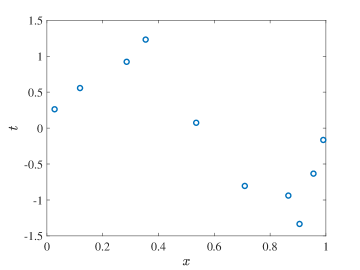
Figure 2.1: Example of a training set $\mathcal{D}$ with $N=10$ points ($x_{n}$,$t_{n}$), $n=1,...,N$.

The outlined learning task is clearly impossible in the absence of additional information on the mechanism relating variables $x$ and $t$. With reference to Fig. 2.1, unless we assume, say, that $x$ and $t$ are related by a function $t=f(x)$ with some properties, such as smoothness, we have no way of predicting the label $t$ for an unobserved domain point $x$. This observation is formalized by the no free lunch theorem to be reviewed in Chapter 5: one cannot learn rules that generalize to unseen examples without making assumptions about the mechanism generating the data. The set of all assumptions made by the learning algorithm is known as the inductive bias.

This discussion points to a key difference between memorizing and learning. While the former amounts to mere retrieval of a value $t_{n}$ corresponding to an already observed pair $(x_{n},t_{n})\in\mathcal{D},$ learning entails the capability to predict the value $t$ for an unseen domain point $x$. Learning, in other words, converts experience – in the form of $\mathcal{D}$ – into expertise or knowledge – in the form of a predictive algorithm. This is well captured by the following quote by Jorge Luis Borges: “To think is to forget details, generalize, make abstractions.” [sevenpilllars].

By and large, the goal of supervised learning is that of identifying a predictive algorithm that minimizes the generalization loss, that is, the error in the prediction of a new label $t$ for an unobserved explanatory variable $x$. How exactly to formulate this problem, however, depends on one’s viewpoint on the nature of the model that is being learned. This leads to the distinction between the frequentist and the Bayesian approaches, which is central to this chapter. As it will be also discussed, the MDL philosophy deviates from the mentioned focus on prediction as the goal of learning, by targeting instead a parsimonious description of the data set $\mathcal{D}$.

2.2 Inference

Before we start our discussion of learning, it is useful to review some basic concepts concerning statistical inference, as they will be needed throughout this chapter and in the rest of this monograph. We specifically consider the inference problem of predicting a rv $\mathrm{t}$ given the observation of another rv $\mathrm{x}$ under the assumption that their joint distribution $p(x,t)$ is known. As a matter of terminology, it is noted that here we will use the term “inference” as it is typically intended in the literature on probabilistic graphical models (see, e.g., [Koller]), hence diverging from its use in other branches of the machine learning literature (see, e.g., [Bishop]).

In order to define the problem of optimal inference, one starts by defining a non-negative loss function $\ell(t,\hat{t})$. This defines the cost, or loss or risk, incurred when the correct value is $t$ while the estimate is $\hat{t}$. An important example is the $\ell_{q}$ loss

$$\ell_{q}(t,\hat{t})=|t-\hat{t}|^{q},$$ (2.1)

which includes as a special case the quadratic loss $\ell_{2}(t,\hat{t})=(t-\hat{t})^{2},$ and the 0-1 loss, or detection error, $\ell_{0}(t,\hat{t})=|t-\hat{t}|_{0},$ where $|a|_{0}=1$ if $a\neq 0$ and $|a|_{0}=0$ otherwise. Once a loss function is selected, the optimal prediction $\hat{t}(x)$ for a given value of the observation $x$ is obtained by minimizing the so-called generalization risk or generalization loss

$$L_{p}(\hat{t})=\textrm{E}_{(\mathrm{x},\mathrm{t})\sim p_{\mathrm{xt}}}[\ell(\mathrm{t},\hat{t}(\mathrm{x}))].$$ (2.2)

The notation $L_{p}$ emphasizes the dependence of the generalization loss on the distribution $p(x,t)$.

The solution of this problem is given by the optimal prediction or decision rule

$$\hat{t}^{*}(x)=\textrm{arg}\min_{\hat{t}}\textrm{E}_{\mathrm{t}\sim p_{\mathrm{t}|\mathrm{x}}}[\ell(\mathrm{t},\hat{t})|x].$$ (2.3)

This can be seen by using the law of iterated expectations $\textrm{E}_{(\mathrm{x},\mathrm{t})\sim p_{\mathrm{xt}}}[\cdot]=\textrm{E}_{\mathrm{x}\sim p_{\mathrm{x}}}[\textrm{E}_{\mathrm{t}\sim p_{\mathrm{t}|\mathrm{x}}}[\cdot|\mathrm{x}]]$. Equation (2.3) shows that the optimal estimate, or prediction, $\hat{t}^{*}(x)$ is a function of the posterior distribution $p(t|x)$ of the label given the domain point $x$ and of the loss function $\ell$. Therefore, once the posterior $p(t|x)$ is known, one can evaluate the optimal prediction (2.3) for any desired loss function, without the need to know the joint distribution $p(x,t)$.

As a special case of (2.3), with the quadratic loss function $\ell_{2}$, the optimal prediction is the conditional mean $\hat{t}^{*}(x)=\textrm{E}_{\mathrm{t}\sim p_{\mathrm{t}|\mathrm{x}}}[\mathrm{t}|x]$; while for the 0-1 loss function $\ell_{0}$, the optimal decision is the mode of the posterior distribution, i.e., $\hat{t}^{*}(x)=\textrm{arg}\max_{t}p(t|x)$.

For example, assume that we have

$$\mathrm{t}|\mathrm{x}=x\sim 0.8\delta(t-x)+0.2\delta(t+x),$$ (2.4)

so that, conditioned on the event $\mathrm{x}=x$, $\mathrm{t}$ equals $x$ with probability 0.8 and $-x$ with probability 0.2. The optimal prediction is $\hat{t}^{*}(x)=0.8x-0.2x=0.6x$ for the quadratic loss, while it is $\hat{t}^{*}(x)=x$ for the 0-1 loss.

The goal of supervised learning methods is broadly speaking that of obtaining a predictor $\hat{t}(x)$ that performs close to the optimal predictor $\hat{t}^{*}(x),$ based only on the training set $\mathcal{D}$, and hence without knowledge of the joint distribution $p(x,t).$ The closeness in performance is measured by the difference between the generalization loss $L_{p}(\hat{t})$ achieved by the trained predictor and the minimum generalization loss $L_{p}(\hat{t}^{*})$ of the optimal predictor, which depends on the true distribution $p(x,t)$. Strictly speaking, this statement applies only for the frequentist approach, which is discussed next. As it will be explained later in the chapter, in fact, while the Bayesian approach still centers around the goal of prediction, its modelling assumptions are different. Furthermore, the MDL approach concentrates on the task of data compression rather than prediction.

2.3 Frequentist Approach

According to the frequentist viewpoint, the training data points $(\mathrm{x}_{n},\mathrm{t}_{n})\in\mathcal{D}$ are independent identically distributed (i.i.d.) rvs drawn from a true, and unknown, distribution $p(x,t)$:

$$(\mathrm{x}_{n},\mathrm{t}_{n})\underset{\textrm{i.i.d.}}{\sim}p(x,t),\textrm{ $i=1,...,N.$}$$ (2.5)

The new observation ($\mathrm{x},\mathrm{t}$) is also independently generated from the same true distribution $p(x,t)$; the domain point $\mathrm{x}$ is observed and the label $\mathrm{t}$ must be predicted. Since the probabilistic model $p(x,t)$ is not known, one cannot solve directly problem (2.3) to find the optimal prediction that minimizes the generalization loss $L_{p}$ in (2.2).

Before discussing the available solutions to this problem, it is worth observing that the definition of the “true” distribution $p(x,t)$ depends in practice on the way data is collected. As in the example of the “beauty AI” context, if the rankings $t_{n}$ assigned to pictures $x_{n}$ of faces are affected by racial biases, the distribution $p(x,t)$ will reflect these prejudices and produce skewed results [beautyai].

Taxonomy of solutions. There are two main ways to address the problem of learning how to perform inference when not knowing the distribution $p(x,t)$:

$\bullet$ Separate learning and (plug-in) inference: Learn first an approximation, say $p_{\mathcal{D}}(t|x)$, of the conditional distribution $p(t|x)$ based on the data $\mathcal{D}$, and then plug this approximation in (2.3) to obtain an approximation of the optimal decision as

$$\hat{t}_{\mathcal{D}}(x)=\textrm{arg}\min_{\hat{t}}\textrm{E}_{\mathrm{t}\sim p_{\mathcal{D}}(t|x)}[\ell(\mathrm{t},\hat{t})|x].$$ (2.6)

$\bullet$ Direct inference via Empirical Risk Minimization (ERM): Learn directly an approximation $\hat{t}_{\mathcal{D}}(\cdot)$ of the optimal decision rule by minimizing an empirical estimate of the generalization loss (2.2) obtained from the data set as

$$\hat{t}_{\mathcal{D}}(\cdot)=\textrm{arg}\min_{\hat{t}}L_{\mathcal{D}}(\hat{t}),$$ (2.7)

where the empirical risk, or empirical loss, is

$$L_{\mathcal{D}}(\hat{t})=\frac{1}{N}\sum_{n=1}^{N}\ell(t_{n},\hat{t}(x_{n})).$$ (2.8)

The notation $L_{\mathcal{D}}(\hat{t})$ highlights the dependence of the empirical loss on the predictor $\hat{t}(\cdot)$ and on the training set $\mathcal{D}.$

In practice, as we will see, both approaches optimize a set of parameters that define the probabilistic model or the predictor. Furthermore, the first approach is generally more flexible, since having an estimate $p_{\mathcal{D}}(t|x)$ of the posterior distribution $p(t|x)$ allows the prediction (2.6) to be computed for any loss function. In contrast, the ERM solution (2.7) is tied to a specific choice of the loss function $\ell$. In the rest of this section, we will start by taking the first approach, and discuss later how this relates to the ERM formulation.

Linear regression example. For concreteness, in the following, we will consider the following running example inspired by [Bishop]. In the example, data is generated according to the true distribution $p(x,t)=p(x)p(t|x)$, where $\mathrm{x}\sim\mathcal{U}(0,1)$ and

$$\mathrm{t}|\mathrm{x}=x\sim\mathcal{N}(\sin(2\pi x),0.1).$$ (2.9)

The training set in Fig. 2.1 was generated from this distribution. If this true distribution were known, the optimal predictor under the $\ell_{2}$ loss would be equal to the conditional mean

$$\hat{t}^{*}(x)=\sin(2\pi x).$$ (2.10)

Hence, the minimum generalization loss is $L_{p}(\hat{t}^{*})=0.1$.

It is emphasized that, while we consider this running example in order to fix the ideas, all the definitions and ideas reported in this chapter apply more generally to supervised learning problems. This will be further discussed in Chapter 4 and Chapter 5.

2.3.1 Discriminative vs. Generative Probabilistic Models

In order to learn an approximation $p_{\mathcal{D}}(t|x)$ of the predictive distribution $p(t|x)$ based on the data $\mathcal{D}$, we will proceed by first selecting a family of parametric probabilistic models, also known as a hypothesis class, and by then learning the parameters of the model to fit (in a sense to be made precise later) the data $\mathcal{D}.$

Consider as an example the linear regression problem introduced above. We start by modelling the label $t$ as a polynomial function of the domain point $x$ added to a Gaussian noise with variance $\beta^{-1}.$ Parameter $\beta$ is the precision, i.e., the inverse variance of the additive noise. The polynomial function with degree $M$ can be written as

$$\mu(x,w)=\sum_{j=0}^{M}w_{j}x^{j}=w^{T}\phi(x),$$ (2.11)

where we have defined the weight vector $w=[w_{0}\textrm{ }w_{1}\cdots w_{M}]^{T}$ and the feature vector $\phi(x)=[1\textrm{ $x\textrm{ $x^{2}$}$}\cdots x^{M}]^{T}$. The vector $w$ defines the relative weight of the powers in the sum (2.11). This assumption corresponds to adopting a parametric probabilistic model $p(t|x,\theta)$ defined as

$$\mathrm{t}|\mathrm{x}=x\sim\mathcal{N}(\mu(x,w),\beta^{-1}),$$ (2.12)

with parameters $\theta=(w\textrm{,$\beta$}).$ Having fixed this hypothesis class, the parameter vector $\theta$ can be then learned from the data $\mathcal{D}$, as it will be discussed.

In the example above, we have parametrized the posterior distribution. Alternatively, we can parametrize, and learn, the full joint distribution $p(x,t)$. These two alternatives are introduced below.

1. Discriminative probabilistic model. With this first class of models, the posterior, or predictive, distribution $p(t|x)$ is assumed to belong to a hypothesis class $p(t|x,\theta)$ defined by a parameter vector $\theta$. The parameter vector $\theta$ is learned from the data set $\mathcal{D}.$ For a given parameter vector $\theta$, the conditional distribution $p(t|x,\theta)$ allows the different values of the label $t$ to be discriminated on the basis of their posterior probability. In particular, once the model is learned, one can directly compute the predictor (2.6) for any loss function.

As an example, for the linear regression problem, once a vector of parameters $\theta_{\mathcal{D}}=(w_{\mathcal{D}},\beta_{\mathcal{D}})$ is identified based on the data $\mathcal{D}$ during learning, the optimal prediction under the $\ell_{2}$ loss is the conditional mean $\hat{t}_{\mathcal{D}}(x)=\textrm{E}_{\mathrm{t}\sim p(t|x,\theta_{\mathcal{D}})}[\mathrm{t}|x]$, that is, $\hat{t}_{\mathcal{D}}(x)=\mu(x,w_{\mathcal{D}})$.

2. Generative probabilistic model. Instead of learning directly the posterior $p(t|x)$, one can model the joint distribution $p(x,t)$ as being part of a parametric family $p(x,t|\theta$). Note that, as opposed to discriminative models, the joint distribution $p(x,t|\theta$) models also the distribution of the covariates $x$. Accordingly, the term “generative” reflects the capacity of this type of models to generate a realization of the covariates x by using the marginal $p(x|\theta).$

Once the joint distribution $p(x,t|\theta$) is learned from the data, one can compute the posterior $p(t|x,\theta)$ using Bayes’ theorem, and, from it, the optimal predictor (2.6) can be evaluated for any loss function. Generative models make stronger assumptions by modeling also the distribution of the explanatory variables. As a result, an improper selection of the model may lead to more significant bias issues. However, there are potential advantages, such as the ability to deal with missing data or latent variables, such as in semi-supervised learning. We refer to Chapter 6 for further discussion (see also [Bishop]).

In the rest of this section, for concreteness, we consider discriminative probabilistic models $p(t|x,\theta)$, although the main definitions will apply also to generative models.

2.3.2 Model Order and Model Parameters

In the linear regression example, the selection of the hypothesis class (2.12) required the definition of the polynomial degree $M$, while the determination of a specific model $p(t|x,\theta)$ in the class called for the selection of the parameter vector $\theta=(w,\beta)$. As we will see, these two types of variables play a significantly different role during learning and should be clearly distinguished, as discussed next.

1. Model order $M$ (and hyperparameters): The model order defines the “capacity” of the hypothesis class, that is, the number of the degrees of freedom in the model. The larger $M$ is, the more capable a model is to fit the available data. For instance, in the linear regression example, the model order determines the size of the weight vector $w$. More generally, variables that define the class of models to be learned are known as hyperparameters. As we will see, determining the model order, and more broadly the hyperparameters, requires a process known as validation.

2. Model parameters $\theta$: Assigning specific values to the model parameters $\theta$ identifies a hypothesis within the given hypothesis class. This can be done by using learning criteria such as Maximum Likelihood (ML) and Maximum a Posteriori (MAP).

We postpone a discussion of validation to the next section, and we start by introducing the ML and MAP learning criteria.

2.3.3 Maximum Likelihood (ML) Learning

Assume now that the model order $M$ is fixed, and that we are interested in learning the model parameters $\theta.$ The ML criterion selects a value of $\theta$ under which the training set $\mathcal{D}$ has the maximum probability of being observed. In other words, the value $\theta$ selected by ML is the most likely to have generated the observed training set. Note that there might be more than one such value.

To proceed, we need to write the probability (density) of the observed labels $t_{\mathcal{D}}$ in the training set $\mathcal{D}$ given the corresponding domain points $x$. Under the assumed discriminative model, this is given as

$$p(t_{\mathcal{D}}|x_{\mathcal{D}},w,\beta) =\prod_{n=1}^{N}p(t_{n}|x_{n},w,\beta),$$ (2.13)

$$=\prod_{n=1}^{N}\mathcal{N}(t_{n}|\mu(x_{n},w),\beta^{-1})$$

where we have used the independence of different data points. Taking the logarithm yields the Log-Likelihood (LL) function

$$\text{}\ln p(t_{\mathcal{D}}|x_{\mathcal{D}},w,\beta) =\sum_{n=1}^{N}\ln p(t_{n}|x_{n},w,\beta)\textrm{ { }}$$

$$=\text{-}\frac{\beta}{2}\sum_{n=1}^{N}(\mu(x_{n},w)-t_{n})^{2}+\frac{N}{2}\ln\frac{\beta}{2\pi}.$$ (2.14)

The LL function should be considered as a function of the model parameters $\theta=(w,\beta)$, since the data set $\mathcal{D}$ is fixed and given. The ML learning problem is defined by the minimization of the Negative LL (NLL) function as

$$\min_{w,\beta}-\frac{1}{N}\sum_{n=1}^{N}\ln p(t_{n}|x_{n},w,\beta).$$ (2.15)

This criterion is also referred to as cross-entropy or log-loss, as further discussed in Sec. 2.6.

If one is only interested in learning only the posterior mean, as is the case when the loss function is $\ell_{2}$, then one can tackle problem (2.14) only over the weights $w$, yielding the optimization

$$\min_{w}L_{\mathcal{D}}(w)=\frac{1}{N}\sum_{n=1}^{N}(\mu(x_{n},w)-t_{n})^{2}.$$ (2.16)

The quantity $L_{\mathcal{D}}(w)$ is known as the training loss. An interesting observation is that this criterion coincides with the ERM problem (2.7) for the $\ell_{2}$ loss if one parametrizes the predictor as $\hat{t}(x)=\mu(x,w)$.

The ERM problem (2.16) can be solved in closed form. To this end, we write the empirical loss as $L_{\mathcal{D}}(w)=N^{-1}||t_{\mathcal{D}}-X_{\mathcal{D}}w||^{2}$, with the $N\times(M+1)$ matrix

$$X_{\mathcal{D}}=[\phi(x_{1})\textrm{ $\phi(x_{2})\cdots$}\phi(x_{N})]^{T}.$$ (2.17)

Its minimization hence amounts to a Least Squares (LS) problem, which yields the solution

$$w_{ML}=(X_{\mathcal{D}}^{T}X_{\mathcal{D}})^{-1}X_{\mathcal{D}}^{T}t_{\mathcal{D}},$$ (2.18)

Note that, in (2.18), we have assumed the typical overdetermined case in which the inequality $N>(M+1)$ holds. More generally, one has the ML solution $w_{ML}=X_{\mathcal{D}}^{\dagger}t_{\mathcal{D}}$. Finally, differentiating the NLL with respect to $\beta$ yields instead the ML estimate

$$\frac{1}{\beta_{ML}}=L_{\mathcal{D}}(w_{ML}).$$ (2.19)

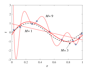
Figure 2.2: Illustration of underfitting and overfitting in ML learning: The dashed line is the optimal predictor (2.10), which depends on the unknown true distribution, while the other lines correspond to the predictor $\hat{t}_{ML}(x)=\mu(x,w_{ML})$ learned via ML with different model orders $M$.

Overfitting and Underfitting. Adopting the $\ell_{2}$ loss, let us now compare the predictor $\hat{t}_{ML}(x)=\mu(x,w_{ML})$ learned via ML with the optimal, but unknown, predictor $\hat{t}^{*}(x)$ in (2.10). To this end, Fig. 2.2 shows the optimal predictor $\hat{t}^{*}(x)$ as a dashed line and the ML-based predictor $\hat{t}_{ML}(x)$ obtained with different values of the model order $M$ for the training set $\mathcal{D}$ in Fig. 2.1 (also shown in Fig. 2.2 for reference).

We begin by observing that, with $M=1$, the ML predictor underfits the data: the model is not rich enough to capture the variations present in the data. As a result, the training loss $L_{\mathcal{D}}(w_{ML})$ in (2.16) is large.

In contrast, with $M=9$, the ML predictor overfits the data: the model is too rich and, in order to account for the observations in the training set, it yields inaccurate predictions outside it. In this case, the training loss $L_{\mathcal{D}}(w)$ in (2.16) is small, but the generalization loss

$$L_{p}(w_{ML})=\textrm{E}_{(\mathrm{x},\mathrm{t})\sim p_{\mathrm{xt}}}[\ell(\mathrm{t},\mu(\mathrm{x},w_{ML}))]$$ (2.20)

is large. With overfitting, the model is memorizing the training set, rather than learning how to generalize to unseen examples.

The choice $M=3$ appears to be the best by comparison with the optimal predictor. Note that this observation is in practice precluded given the impossibility to determine $\hat{t}^{*}(x)$ and hence the generalization loss. We will discuss below how to estimate the generalization loss using validation.

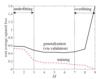
Figure 2.3: Square root of the generalization loss $L_{p}(w_{ML})$ and of the training loss $L_{\mathcal{D}}(w_{ML})$ as a function of the model order $M$ for the training data set in Fig. 2.1.

The impact of the model order $M$ on training and generalization losses is further elaborated on in Fig. 2.3, which shows the squared root of the generalization loss $L_{p}(w_{ML})$ and of the training loss $L_{\mathcal{D}}(w_{ML})$ as a function of $M$ for the same training data set. A first remark is that, as expected, the training loss is smaller than the generalization loss, since the latter accounts for all pairs ($\mathrm{x},\mathrm{t}$)$\sim p(x,t)$, while the former includes only the training points used for learning. More importantly, the key observation here is that increasing $M$ allows one to better fit – and possibly overfit – the training set, hence reducing $L_{\mathcal{D}}(w_{ML})$. The generalization loss $L_{p}(w_{ML})$ instead tends to decrease at first, as we move away from the underfitting regime, but it eventually increases for sufficiently large $M$. The widening of the gap between training and generalization provides evidence that overfitting is occurring. From Fig. 2.3, we can hence conclude that, in this example, model orders larger than $M=7$ should be avoided since they lead to overfitting, while model order less than $M=3$ should also not be considered in order to avoid underfitting.

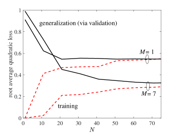
Figure 2.4: Square root of the generalization loss $L_{p}(w_{ML})$ and of the training loss $L_{\mathcal{D}}(w_{ML})$ as a function of the training set size $N$. The asymptote of the generalization and training losses is given by the minimum generalization loss $L_{p}(w^{*})$ (cf. (2.21)) achievable for the given model order (see Fig. 2.5).

What if we had more data? Extrapolating from the behavior observed in Fig. 2.2, we can surmise that, as the number $N$ of data points increases, overfitting is avoided even for large values of $M$. In fact, when the training set is big as compared to the number of parameters in $\theta$, we expect the training loss $L_{\mathcal{D}}(w)$ to provide an accurate measure of the generalization loss $L_{p}(w)$ for all possible values of $w$. Informally, we have the approximation $L_{\mathcal{D}}(w)\simeq L_{p}(w)$ simultaneously for all values of $w$ as long as $N$ is large enough. Therefore, the weight vector $w_{ML}$ that minimizes the training loss $L_{\mathcal{D}}(w)$ also (approximately) minimizes the generalization loss $L_{p}(w)$. It follows that, for large $N$, the ML parameter vector $w_{ML}$ tends to the the optimal value $w^{*}$ (assuming for simplicity of argument that it is unique) that minimizes the generalization loss among all predictors in the model, i.e.,

$$w^{*}=\textrm{arg}\underset{w}{\textrm{min }}L_{p}(w).$$ (2.21)

This discussion will be made precise in Chapter 5.

To offer numerical evidence for the point just made, Fig. 2.4 plots the (square root of the) generalization and training losses versus $N$, where the training sets were generated at random from the true distribution. From the figure, we can make the following important observations. First, overfitting – as measured by the gap between training and generalization losses – vanishes as $N$ increases. This is a consequence of the discussed approximate equalities $L_{\mathcal{D}}(w)\simeq L_{p}(w)$ and $w_{ML}\simeq w^{*}$, which are valid as $N$ grows large, which imply the approximate equalities $L_{\mathcal{D}}(w_{ML})\simeq L_{p}(w_{ML})\simeq L_{p}(w^{*})$.

Second, it is noted that the training loss $L_{\mathcal{D}}(w_{ML})$ tends to the minimum generalization loss $L_{p}(w^{*})$ for the given $M$ from below, while the generalization loss $L_{p}(w_{ML})$ tends to it from above. This is because, as $N$ increases, it becomes more difficult to fit the data set $\mathcal{D}$, and hence $L_{\mathcal{D}}(w_{ML})$ increases. Conversely, as $N$ grows large, the ML estimate becomes more accurate, because of the increasingly accurate approximation $w_{ML}\simeq w^{*}$, and thus the generalization loss $L_{p}(w_{ML})$ decreases.

Third, selecting a smaller model order $M$ yields an improved generalization loss when the training set is small, while a larger value of $M$ is desirable when the data set is bigger. In fact, as further discussed below, when $N$ is small, the estimation error caused by overfitting dominates the bias caused by the choice of a small hypothesis class. In contrast, for sufficiently large training sets, the estimation error vanishes and the performance is dominated by the bias induced by the selection of the model.

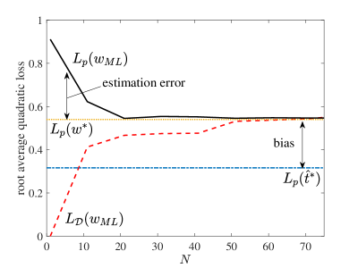
Figure 2.5: Illustration of the bias and training error based on the decomposition (2.22).

Bias and generalization gap. The previous paragraph introduced the notions of estimation error and bias associated with the selection of a given model order $M$. While Chapter 5 will provide a more extensive discussion on these concepts, it is useful to briefly review them here in the context of ML learning. Estimation error and bias refer to the following decomposition of the generalization loss achieved by the given solution $w_{ML}$

$$L_{p}(w_{ML})=L_{p}(\hat{t}^{*})+(L_{p}(w^{*})-L_{p}(\hat{t}^{*}))+(L_{p}(w_{ML})-L_{p}(w^{*})).$$ (2.22)

This decomposition is illustrated in Fig. 2.5 for $M=1$. In (2.22), the term $L_{p}(\hat{t}^{*})=0.1$ (the figure shows the square root) is, as seen, the minimum achievable generalization loss without any constraint on the hypothesis class. The term $(L_{p}(w^{*})-L_{p}(\hat{t}^{*}))$ represents the bias, or approximation error, caused by the choice of the given hypothesis class, and hence also by the choice of $M$. This is because, by (2.21), $L_{p}(w^{*})$ is the best generalization loss for the given model. Recall that the loss $L_{p}(w^{*})$ can be achieved when $N$ is large enough. Finally, the term $(L_{p}(w_{ML})-L_{p}(w^{*}))$ is the estimation error or generalization gap that is incurred due to the fact that $N$ is not large enough and hence we have $w_{ML}\neq w^{*}$.

From the decomposition (2.22), a large $N$ allows us to reduce the estimation error, but it has no effect on the bias. This is seen in Fig. 2.4, where the asymptote achieved by the generalization loss as $N$ increases equals the minimum generalization loss $L_{p}(w^{*})$ for the given model order. Choosing a small value of $M$ in the regime of large data imposes a floor on the achievable generalization loss that no amount of additional data can overcome.

Validation and testing. In the discussion above, it was assumed that the generalization loss $L_{p}(w)$ can somehow be evaluated. Since this depend on the true unknown distribution $p(x,t)$, this evaluation is, strictly speaking, not possible. How then to estimate the generalization loss in order to enable model order selection using a plot as in Fig. 2.3? The standard solution is to use validation.

The most basic form of validation prescribes the division of the available data into two sets: a hold-out, or validation, set and the training set. The validation set is used to evaluate an approximation of the generalization loss $L_{p}(w)$ via the empirical average

$$L_{p}(w)\simeq\frac{1}{N_{v}}\sum_{n=1}^{N_{v}}\ell(t_{n},\mu(x_{n},w)),$$ (2.23)

where the sum is done over the $N_{v}$ elements of the validation set.

The just described hold-out approach to validation has a clear drawback, as part of the available data needs to be set aside and not used for training. This means that the number of examples that can be used for training is smaller than the number of overall available data points. To partially obviate this problem, a more sophisticated, and commonly used, approach to validation is $k$-fold cross-validation. With this method, the available data points are partitioned, typically at random, into $k$ equally sized subsets. The generalization loss is then estimated by averaging $k$ different estimates. Each estimate is obtained by retaining one of the $k$ subsets for validation and the remaining $k-1$ subsets for training. When $k=N$, this approach is also known as leave-one-out cross-validation.

Test set. Once a model order $M$ and model parameters $\theta$ have been obtained via learning and validation, one typically needs to produce an estimate of the generalization loss obtained with this choice ($M,\theta$). The generalization loss estimated via validation cannot be used for this purpose. In fact, the validation loss tends to be smaller than the actual value of the generalization loss. After all, we have selected the model order so as to yield the smallest possible error on the validation set. The upshot is that the final estimate of the generalization loss should be done on a separate set of data points, referred to as the test set, that are set aside for this purpose and not used at any stage of learning. As an example, in competitions among different machine learning algorithms, the test set is kept by a judge to evaluate the submissions and is never shared with the contestants.

2.3.4 Maximum A Posteriori (MAP) Criterion

We have seen that the decision regarding the model order $M$ in ML learning concerns the tension between bias, whose reduction calls for a larger $M$, and estimation error, whose decrease requires a smaller $M$. ML provides a single integer parameter, $M$, as a gauge to trade off bias and estimation error. As we will discuss here, the MAP approach and, more generally, regularization, enable a finer control of these two terms. The key idea is to leverage prior information available on the behavior of the parameters in the absence, or presence, of overfitting.

To elaborate, consider the following experiment. Evaluate the ML solution $w_{ML}$ in (2.18) for different values of $M$ and observe how it changes as we move towards the overfitting regime by increasing $M$ (see also [Bishop, Table 1.1]). For the experiment reported in Fig. 2.2, we obtain the following values: for $M=1$, $w_{ML}=[0.93\textrm{, }-1.76]^{T}$; for $M=3$, $w_{ML}=[-0.28,\textrm{ }13.32,\textrm{ }-35.92,\textrm{ }22.56]^{T}$; and for $M=9$, $w_{ML}=[$$13.86$, $-780.33,$ $12.99$$\times 10^{3},$ $-99.27\times 10^{3},$ $416.49\times 10^{3},$ $-1.03\times 10^{6},$ $1.56\times 10^{6},$ $1.40\times 10^{6},$ $0.69\times 10^{6},$ $-1.44\times 10^{6}]$. These results suggest that a manifestation of overfitting is the large value of norm $\left\|w\right\|$ of the vector of weights. We can use this observation as prior information, that is as part of the inductive bias, in designing a learning algorithm.

To this end, we can impose a prior distribution on the vector of weights that gives lower probability to large values. A possible, but not the only, way to do this is to is to assume a Gaussian prior as

$$w\sim\mathcal{N}(0,\alpha^{-1}I),$$ (2.24)

so that all weights are a priori i.i.d. zero-mean Gaussian variables with variance $\alpha^{-1}$. Increasing $\alpha$ forces the weights to be smaller as it reduces the probability associated with large weights. The precision variable $\alpha$ is an example of a hyperparameter. In a Bayesian framework, hyperparameters control the distribution of the model parameters. As anticipated, hyperparameters are determined via validation.

Rather than maximizing the LL, that is, probability density  $p(t_{\mathcal{D}}|x_{\mathcal{D}},w,\beta)$ of the labels in the training set, as for ML, the MAP criterion prescribes the maximization of the joint probability distribution of weights and of labels given the prior $p(w)=\mathcal{N}(w|0,\alpha^{-1}I)$, that is,

$$p(t_{\mathcal{D}},w|x_{\mathcal{D}},\beta)=p(w)\prod_{n=1}^{N}p(t_{n}|x_{n},w,\beta).$$ (2.25)

Note that a prior probability can also be assumed for the parameter $\beta$, but in this example we leave $\beta$ as a deterministic parameter. The MAP learning criterion can hence be formulated as

$$\min_{w,\beta}-\sum_{n=1}^{N}\ln p(t_{n}|x_{n},w,\beta)-\ln p(w).$$ (2.26)

The name “Maximum a Posteriori” is justified by the fact that problem (2.26) is equivalent to maximizing the posterior distribution of the parameters $w$ given the available data, as we will further discuss in the next section. This yields the following problem for the weight vector

$$\min_{w}L_{\mathcal{D}}(w)+\frac{\lambda}{N}\|w\|^{2},$$ (2.27)

where we have defined $\lambda=\alpha/\beta$ and we recall that the training loss is $L_{\mathcal{D}}(w)=N^{-1}\left\|t_{\mathcal{D}}-X_{\mathcal{D}}w\right\|^{2}.$

ML vs. MAP. Observing (2.27), it is important to note the following general property of the MAP solution: As the number $N$ of data points grows large, the MAP estimate tends to the ML estimate, given that the contribution of the prior information term decreases as $1/N$. When $N$ is large enough, any prior credence is hence superseded by the information obtained from the data.

Problem (2.27), which is often referred to as ridge regression, modifies the ML criterion by adding the quadratic (or Tikhonov) regularization function

$$R(w)=\|w\|^{2}$$ (2.28)

multiplied by the term $\lambda/N.$ The regularization function forces the norm of the solution to be small, particularly with larger values of the hyperparameter $\lambda$, or equivalently $\alpha$. The solution of problem (2.27) can be found by using standard LS analysis, yielding

$$w_{MAP}=(\lambda I+X_{\mathcal{D}}^{T}X_{\mathcal{D}})^{-1}X_{\mathcal{D}}^{T}t_{\mathcal{D}}.$$ (2.29)

This expression confirms that, as $N$ grows large, the term $\lambda I$ becomes negligible and the solution tends to the ML estimate (2.18) (see [lehmann2006theory] for a formal treatment).

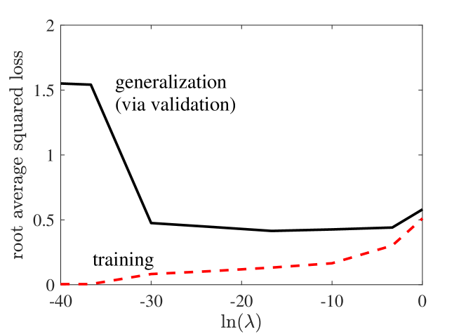
Figure 2.6: Square root of the generalization loss $L_{p}(w_{MAP})$ and of the training loss $L_{\mathcal{D}}(w_{MAP})$ as a function of the regularization parameter $\lambda$ for the training data set in Fig. 2.1 with $M=9$.

Fig. 2.6 shows the squared root of the generalization loss $L_{p}(w_{MAP})$ and of the training loss $L_{\mathcal{D}}(w_{MAP})$ as a function of $\lambda$ (in logarithmic scale) for the training data set in Fig. 2.1 with $M=9$. The generalization loss is estimated using validation. We observe that increasing $\lambda$, and hence the relevance of the regularization term, has a similar impact as decreasing the model order $M$. A larger $\lambda$ reduces the effective capacity of the model. Stated in different words, increasing $\lambda$ reduces overfitting but may entail a larger bias.

Other standard examples for the prior distribution include the Laplace pdf, which yields the $l_{1}$ norm regularization function $R(w)=\left\|w\right\|_{1}=\sum_{j=0}^{M}\left|w\right|_{1}$. This term promotes the sparsity of the solution, which is useful in many signal recovery algorithms [baraniuk2007compressive] and in non-parametric function estimation [tsybakov2009introduction]. The corresponding optimization problem

$$\min_{w}L_{\mathcal{D}}(w)+\frac{\lambda}{N}\|w\|_{1}$$ (2.30)

is known as LASSO (Least Absolute Shrinkage and Selection Operator).

2.3.5 Regularization

We have seen above that the MAP learning criterion amounts to the addition of a regularization function $R(w)$ to the ML or ERM learning losses. This function penalizes values of the weight vector $w$ that are likely to occur in the presence of overfitting, or, generally, that are improbable on the basis of the available prior information. The net effect of this addition is to effectively decrease the capacity of the model, as the set of values for the parameter vector $w$ that the learning algorithm is likely to choose from is reduced. As a result, as seen, regularization can control overfitting and its optimization requires validation.

Regularization generally refers to techniques that aim at reducing overfitting during training. The discussion in the previous subsection has focused on a specific form of regularization that is grounded in a probabilistic interpretation in terms of MAP learning. We note that the same techniques, such as ridge regression and LASSO, can also be introduced independently of a probabilistic framework in an ERM formulation. Furthermore, apart from the discussed addition of regularization terms to the empirical risk, there are other ways to perform regularization.

One approach is to modify the optimization scheme by using techniques such as early stopping [Goodfellowbook]. Another is to augment the training set by generating artificial examples and hence effectively increasing the number $N$ of training examples. Related to this idea is the technique known as bagging. With bagging, we first create a number $K$ of bootstrap data sets. Bootstrap data sets are obtained by selecting $N$ data points uniformly with replacement from $\mathcal{D}$ (so that the same data point generally appears multiple times in the bootstrap data set). Then, we train the model $K$ times, each time over a different bootstrap set. Finally, we average the results obtained from the models using equal weights. If the errors accrued by the different models were independent, bagging would yield an estimation error that decreases with $K$. In practice, significantly smaller gains are obtained, particularly for large $K$, given that the bootstrap data sets are all drawn from $\mathcal{D}$ and hence the estimation errors are not independent [Bishop].

2.4 Bayesian Approach

The frequentist approaches discussed in the previous section assume the existence of a true distribution, and aim at identifying a specific value for the parameters $\theta$ of a probabilistic model to derive a predictor (cf. (2.3)). ML chooses the value $\theta$ that maximizes the probability of the training data, while MAP includes in this calculation also prior information about the parameter vector. With the frequentist approach, there are hence two distributions on the data: the true distribution, approximated by the empirical distribution of the data and the model (see further discussion in Sec. 2.8).

The Bayesian viewpoint is conceptually different: (i) It assumes that all data points are jointly distributed according to a distribution that is known except for some hyperparameters; and (ii) the model parameters $\theta$ are jointly distributed with the data. As a result, as it will be discussed, rather than committing to a single value to explain the data, the Bayesian approach considers the explanations provided by all possible values of $\theta$, each weighted according to a generally different, and data-dependent, “belief”.

More formally, the Bayesian viewpoint sees the vector of parameters as rvs that are jointly distributed with the labels $\mathrm{t}_{\mathcal{D}}$ in the training data $\mathcal{D}$ and with the new example $\mathrm{t}$. We hence have the joint distribution $p(t_{\mathcal{D}},w,t|x_{\mathcal{D}},x)$. We recall that the conditioning on the domain points $x_{\mathcal{D}}$ and $x$ in the training set and in the new example, respectively, are hallmarks of discriminative probabilistic models. The Bayesian solution simply takes this modeling choice to its logical end point: in order to predict the new label $\mathrm{t}$, it directly evaluates the posterior distribution $p(t|x_{\mathcal{D}},t_{\mathcal{D}},x)=p(t|\mathcal{D},x)$ given the available information ($\mathcal{D},x$) by applying the marginalization rules of probability to the joint distribution $p(t_{\mathcal{D}},w,t|x_{\mathcal{D}},x)$.

As seen, the posterior probability $p(t|\mathcal{D},x)$ can be used as the predictive distribution in (2.3) to evaluate a predictor $\hat{t}(x)$. However, a fully Bayesian solution returns the entire posterior $p(t|\mathcal{D},x)$, which provides significantly more information about the unobserved label $\mathrm{t}$. As we will discuss below, this knowledge, encoded in the posterior $p(t|\mathcal{D},x)$, combines both the assumed prior information about the weight vector $w$ and the information that is obtained from the data $\mathcal{D}$.

To elaborate, in the rest of this section, we assume that the precision parameter $\beta$ is fixed and that the only learnable parameters are the weights in vector $w$. The joint distribution of the labels in the training set, of the weight vector and of the new label, conditioned on the domain points $x_{\mathcal{D}}$ in the training set and on the new point $x$, is given as

$$p(t_{\mathcal{D}},w,t|x_{\mathcal{D}},x)=\underbrace{p(w)}_{\text{a priori distribution}}\underbrace{p(t_{\mathcal{D}}|x_{\mathcal{D}},w)}_{\text{ likelihood}}\underbrace{p(t|x,w)}_{\text{ distribution of new data}}.$$ (2.31)

In the previous equation, we have identified the a priori distribution of the data; the likelihood term $p(t_{\mathcal{D}}|x_{\mathcal{D}},w)=\prod_{n=1}^{N}\mathcal{N}(t_{n}|\mu(x_{n},w),\beta^{-1})$ in (2.13); and the pdf of the new label $p(t|w,x)=\mathcal{N}(t|\mu(x,w),\beta^{-1})$. It is often useful to drop the dependence on the domain points $x_{\,\mathcal{D}}$ and $x$ to write only the joint distribution of the random variables in the model as

$$p(t_{\mathcal{D}},w,t)=\underbrace{p(w)}_{\text{a priori distribution}}\underbrace{p(t_{\mathcal{D}}|w)}_{\text{ likelihood}}\underbrace{p(t|w)}_{\text{ distribution of new data}}.$$ (2.32)

This factorization can be represented graphically by the Bayesian Network (BN) in Fig. 2.7. The significance of the graph should be clear by inspection, and it will be discussed in detail in Chapter 7.

It is worth pointing out that, by treating all quantities in the model – except for the hyperparameter $\alpha$ – as rvs, the Bayesian viewpoint does away with the distinction between learning and inference. In fact, since the joint distribution is assumed to be known in a Bayesian model, the problem at hand becomes that of inferring the unknown rv $\mathrm{t}$. To restate this important point, the Bayesian approach subsumes all problems in the general inference task of estimating a subset of rvs given other rvs in a set of jointly distributed rvs with a known joint distribution.

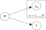
Figure 2.7: Bayesian Network (BN) describing the joint distribution (2.32) of the weight vector $\mathrm{w}$, of the labels $\mathrm{t}_{\mathcal{D}}$ in the training data $\mathcal{D}$ and $\mathrm{t}$ in the new example, as used in the Bayesian approach.

As mentioned, we are interested in computing the posterior probability $p(t|\mathcal{D},x)$ of the new label $\mathrm{t}$ given the training data $\mathcal{D}$ and the new domain point $\mathrm{x}=x$. Dropping again the domain variables to simplify the notation, we apply standard rules of probability to obtain

$$p(t|t_{\mathcal{D}})=\frac{p(t_{\mathcal{D}},t)}{p(t_{\mathcal{D}})}=\int\frac{p(w)p(t_{\mathcal{D}}|w)}{p(t_{\mathcal{D}})}p(t|w)dw$$

$$=\int p(w|t_{\mathcal{D}})p(t|w)dw,$$ (2.33)

where the second equality follows from the marginalization rule $p(t_{\mathcal{D}},t)=\int p(t_{\mathcal{D}},w,t)dw$ and the last equality from Bayes’ theorem. Putting back the dependence on the domain variables, we obtain the predictive distribution as

$$p(t|x,\mathcal{D})=\int\underbrace{p(w|\mathcal{D})}_{\text{posterior distribution of $w$}}p(t|x,w)dw.$$ (2.34)

This is the key equation. Accordingly, the Bayesian approach considers the predictive probability $p(t|x,w)$ associated with each value of the weight vector $w$ weighted by the posterior belief

$$p(w|\mathcal{D})=\frac{p(w)p(t_{\mathcal{D}}|x_{\mathcal{D}},w)}{p(t_{\mathcal{D}}|x_{\mathcal{D}})}.$$ (2.35)

The posterior belief $p(w|\mathcal{D})$, which defines the weight of the parameter vector $w,$ is hence proportional to the prior belief $p(w)$ multiplied by the correction $p(t_{\mathcal{D}}|x_{\mathcal{D}},w)$ due to the observed data.

Computing the posterior $p(w|\mathcal{D})$, and a fortiori also the predictive distribution $p$$(t|x,\mathcal{D})$, is generally a difficult task that requires the adoption of approximate inference techniques covered in Chapter 8. For this example, however, we can directly compute the predictive distribution as [Bishop]

$$t|x,\mathcal{D}\sim\mathcal{N}(\mu(x,w_{MAP}),s^{2}(x)),$$ (2.36)

where $s^{2}(x)=\beta^{-1}(1+\phi(x)^{T}\left(\lambda I+X_{\mathcal{D}}^{T}X_{\mathcal{D}}\right)^{-1}\phi(x)).$ Therefore, in this particular example, the optimal predictor under $\ell_{2}$ loss is MAP. This is consequence of the fact that mode and mean of a Gaussian pdf coincide, and is not a general property. Even so, as discussed next, the Bayesian viewpoint can provide significantly more information on the label $t$ than the ML or MAP.

ML and MAP vs. Bayesian approach. The Bayesian posterior (2.36) provides a finer prediction of the labels $t$ given the explanatory variables $x$ as compared to the predictive distribution $p(t|x,\theta_{ML})=\mathcal{N}(\mu(x,w_{ML}),\beta^{-1})$ returned by ML and similarly by MAP. To see this, note that the latter has the same variance for all values of $x$, namely $\beta^{-1}.$ Instead, the Bayesian approach reveals that, due to the uneven distribution of the observed values of $x$, the accuracy of the prediction of labels depends on the value of $x$: Values of $x$ closer to the existing points in the training sets generally exhibit a smaller variance.

This is shown in Fig. 2.8, which plots a training set, along with the corresponding predictor $\mu(x,w_{MAP})$ and the high-probability interval $\mu(x,w_{MAP})\pm s(x)$ produced by the Bayesian method. We set $M=9$, $\beta^{-1}=0.1$ and $\alpha^{-1}=0.2\times 10^{5}.$ For reference, we also show the interval $\mu(x,w_{MAP})\pm\beta^{-1/2}$ that would result from the MAP analysis. This intervals illustrate the capability of the Bayesian approach to provide information about the uncertainty associated with the estimate of $t$.

This advantage of the Bayesian approach reflects its conceptual difference with respect to the frequentist approach: The frequentist predictive distribution refers to a hypothetical new observation generated with the same mechanism as the training data; instead, the Bayesian predictive distribution quantifies the statistician’s belief in the value of $t$ given the assumed prior and the training data.

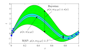
Figure 2.8: Illustration of the predictive distribution $p(t|x,\mathcal{D})$ produced by the Bayesian method for the training set shown in the figure as compared to that obtained with the MAP criterion. The larger interval corresponds to $\mu(x,w_{MAP})\pm s(x)$ for the Bayesian method, while the smaller interval to $\mu(x,w_{MAP})\pm\beta^{-1/2}$ for MAP ($M=9$, $\beta^{-1}=0.1$ and $\alpha^{-1}=0.2\times 10^{5}$).

From (2.36), we can make another important general observation about the relationship with ML and MAP concerning the asymptotic behavior when $N$ is large. In particular, when $N\rightarrow\infty$, we have already seen that, informally, the limit $w_{MAP}\rightarrow w_{ML}$ holds. We now observe that it is also the case that the variance $s^{2}(x)$ of the Bayesian predictive distribution tends to $\beta^{-1}.$ As a result, we can conclude that the Bayesian predictive distribution approaches that returned by ML when $N$ is large. A way to think about this conclusion is that, when $N$ is large, the posterior distribution $p(w|\mathcal{D})$ of the weights tends to concentrate around the ML estimate, hence limiting the average (2.34) to the contribution of the ML solution.

Marginal likelihood. Another advantage of the Bayesian approach is that, in principle, it allows model selection to be performed without validation. Toward this end, compute the marginal likelihood

$$p(t_{\mathcal{D}}|x_{\mathcal{D}})=\int p(w)\prod_{n=1}^{N}p(t_{n}|x_{n},w)dw,$$ (2.37)

that is, the probability density of the training set when marginalizing over the weight distribution. With the ML approach, the corresponding quantity $p(t_{\mathcal{D}}|x_{\mathcal{D}},w_{ML})$ can only increase by choosing a larger model order $M$. In fact, a larger $M$ entails more degrees of freedom in the optimization (2.16) of the LL. A similar discussion applies also to MAP. However, this is not the case for (2.37): a larger $M$ implies a more “spread-out” prior distribution of the weights, which may result in a more diffuse distribution of the labels in (2.37). Hence, increasing $M$ may yield a smaller marginal likelihood.

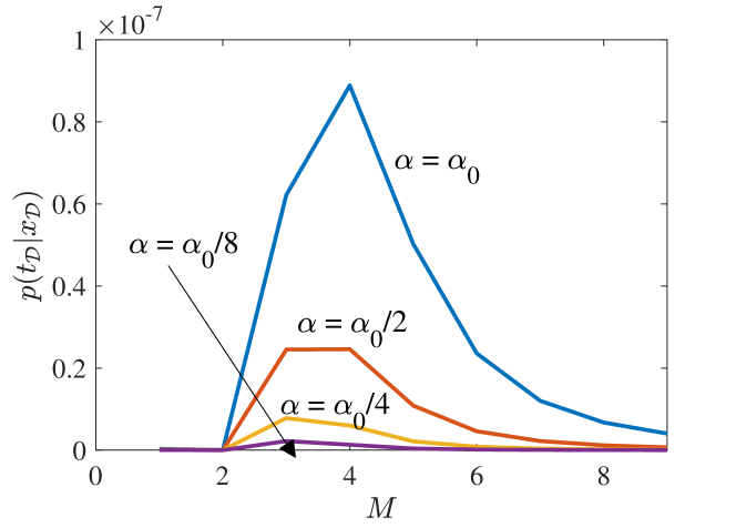
Figure 2.9: Marginal likelihood versus the model order $M$ for the training set of Fig. 2.1 ($\beta=10$, $\alpha_{0}=10^{-3}$).

To illustrate this point, Fig. 2.9 plots the marginal likelihood for the data set in Fig. 2.1 for $\beta=10$ and three different values of $\alpha$ as a function of $M$. The marginal likelihood in this example can be easily computed since we have

$$\mathrm{t_{\mathcal{D}}}|\mathrm{x_{\mathcal{D}}}=x_{\mathcal{D}}\sim\mathcal{N}(0,\alpha^{-1}X_{\mathcal{D}}X_{\mathcal{D}}^{T}+\beta^{-1}I).$$ (2.38)

It is observed that the marginal likelihood presents a peak at a given value of $M$, while decreasing when moving away from the optimal value. Therefore, we could take the value of $M$ at which the marginal likelihood is maximized as the selected model order.

Does this mean that validation is really unnecessary when adopting a Bayesian viewpoint? Unfortunately, this is not necessarily the case. In fact, one still needs to set the hyperparameter $\alpha$. As seen in Fig. 2.9, varying $\alpha$ can lead to different conclusions on the optimal value of $M$. An alternative approach would be to treat $\alpha$, and even $M$, as rvs with given priors to be specified (see, e.g., [MarcoScutari]). This would not obviate the problem of selecting hyperparameters – now defining the prior distributions of $\alpha$ and $M$ – but it can lead to powerful hierarchical models. The necessary tools will be discussed in Chapter 7.

As a final note, rather than using often impractical exhaustive search methods, the optimization over the hyperparameters and the model order $M$ for all criteria discussed so far, namely ML, MAP and Bayesian, can be carried out using so-called Bayesian optimization tools [Bayesianopt]. A drawback of these techniques is that they have their own hyperparameters that need to be selected.

Empirical Bayes. Straddling both frequentist and Bayesian viewpoints is the so-called empirical Bayes method. This approach assumes an a priori distribution for the parameters, but then estimates the parameters of the prior – say mean and variance of a Gaussian prior – from the data [efron2016computer].

2.5 Minimum Description Length (MDL)^∗

In this section, we briefly introduce a third, conceptually distinct, learning philosophy – the MDL criterion. The reader is warned that the treatment here is rather superficial, and that a more formal definition of the MDL criterion would would require a more sophisticated discussion, which can be found in [Grunwald]. Furthermore, some background in information theory is preferable in order to fully benefit from this discussion.

To start, we first recall from the treatment above that learning requires the identification of a model, or hypothesis class – here the model order $M$ – and of a specific hypothesis, defined by parameters $\theta$ – here $\theta=(w,\beta)$ – within the class. While MDL can be used for both tasks, we will focus here only on the first.

To build the necessary background, we now need to review the relationship between probabilistic models and compression. To this end, consider a signal $x$ taking values in a finite alphabet $\mathcal{X}$, e.g., a pixel in a gray scale image. Fix some probability mass function (pmf) $p(x)$ on this alphabet. A key result in information theory states that it is possible to design a lossless compression scheme that uses $\left\lceil-\log p(x)\right\rceil$ bits to represent value $x$

By virtue of this result, the choice of a probability distribution $p(x)$ is akin to the selection of a lossless compression scheme that produces a description of around $-\log p(x)$ bits to represent value $x$. Note that the description length $-\log p(x)$ decreases with the probability assigned by $p(x)$ to value $x$: more likely values under $p(x)$ are assigned a smaller description. Importantly, a decoder would need to know $p(x)$ in order to recover $x$ from the bit description.

At an informal level, the MDL criterion prescribes the selection of a model that compresses the training data to the shortest possible description. In other words, the model selected by MDL defines a compression scheme that describes the data set $\mathcal{D}$ with the minimum number of bits. As such, the MDL principle can be thought of as a formalization of Occam’s razor: choose the model that yields the simplest explanation of the data. As we will see below, this criterion naturally leads to a solution that penalizes overfitting.

What is the length of the description of a data set $\mathcal{D}$ that results from the selection of a specific value of $M$? The answer is not straightforward, since, for a given value of $M$, there are as many probability distributions as there are values for the corresponding parameters $\theta$ to choose from. A formal calculation of the description length would hence require the introduction of the concept of universal compression for a given probabilistic model [Grunwald]. Here, we will limit ourselves to a particular class of universal codes known as two-part codes.

Using two-part codes, we can compute the description length for the data $\mathcal{D}$ that results from the choice of a model order $M$ as follows. First, we obtain the ML solution ($w_{ML},\beta_{ML}$). Then, we describe the data set by using a compression scheme defined by the probability $p(t|x,w_{ML},\beta_{ML})=\mathcal{N}(t|\mu(x,w_{ML}),\beta_{ML}^{-1})$. As discussed, this produces a description of approximately $-\sum_{n=1}^{N}\textrm{log}p(t_{n}|x_{n},w_{ML},\beta_{ML})$ bits. This description is, however, not sufficient, since the decoder of the description should also be informed about the parameters $(w_{ML},\beta_{ML}$).

Using quantization, the parameters can be described by means of a number $C(M)$ of bits that is proportional to the number of parameters, here $M+2.$ Concatenating these bits with the description produced by the ML model yields the overall description length

$$-\sum_{n=1}^{N}\textrm{log}p(t_{n}|x_{n},w_{ML},\beta_{ML})+C(M).$$ (2.39)

MDL – in the simplified form discussed here – selects the model order $M$ that minimizes the description length (2.39). Accordingly, the term $C(M)$ acts as a regularizer. The optimal value of $M$ for the MDL criterion is hence the result of the trade-off between the minimization of the overhead $C(M)$, which calls for a small value of $M$, and the minimization of the NLL, which decreases with $M$.

Under some technical assumptions, the overhead term can be often evaluated in the form $(K/2)\ln N+c$, where $K$ is the number of parameters in the model and $c$ is a constant. This expression is not quite useful in practice, but it provides intuition about the mechanism used by MDL to combat overfitting.

2.6 Information-Theoretic Metrics

We now provide a brief introduction to information theoretic metrics by leveraging the example studied in this chapter. As we will see in the following chapters, information-theoretic metrics are used extensively in the definition of learning algorithms. Appendix A provides a detailed introduction to information-theoretic measures in terms of inferential tasks. Here we introduce the key metrics of Kullback-Leibler (KL) divergence and entropy by examining the asymptotic behavior of ML in the regime of large $N$. The case with finite $N$ is covered in Chapter 6 (see Sec. 6.4.3).

To start, we revisit the ML problem (2.15), which amounts to the minimization of the NLL $-N^{-1}\sum_{n=1}^{N}\ln p(t_{n}|x_{n},w,\beta)$, also known as log-loss. According to the frequentist viewpoint, the training set variables are drawn i.i.d. according to the true distribution $p(x,t)$, i.e., $(\mathrm{x}_{n},\mathrm{t}_{n})\sim p_{\mathrm{xt}}$ i.i.d. over $n=1,...,N$. By the strong law of large numbers, we then have the following limit with probability one

$$-\frac{1}{N}\sum_{n=1}^{N}\ln p(\mathrm{t}_{n}|\mathrm{x}_{n},w,\beta)\rightarrow\textrm{E}_{(\mathrm{x},\mathrm{t})\sim p_{\mathrm{xt}}}\left[-\ln p(\mathrm{t}|\mathrm{x},w,\beta)\right].$$ (2.40)

As we will see next, this limit has a useful interpretation in terms of the KL divergence.

The KL divergence between two distributions $p$ and $q$ is defined as

$$\textrm{KL}(p\|q)=\textrm{E}_{\mathrm{x}\sim p_{\mathrm{x}}}\left[\ln\frac{p(\mathrm{x})}{q(\mathrm{x})}\right].$$ (2.41)

The KL divergence is hence the expectation of the Log-Likelihood Ratio (LLR) $\ln(p(x)/q(x))$ between the two distributions, where the expectation is taken with respect to the distribution at the numerator. The LLR tends to be larger, on average, if the two distributions differ more significantly, while being uniformly zero only when the two distributions are equal. Therefore, the KL divergence measures the “distance” between two distributions. As an example, with $p(x)=\mathcal{N}(x|\mu_{1},\sigma_{1}^{2})$ and $q(x)=\mathcal{N}(x|\mu_{2},\sigma_{2}^{2})$, we have

$$\textrm{KL}(p\|q)=\frac{1}{2}\left(\frac{\sigma_{1}^{2}}{\sigma_{2}^{2}}+\frac{(\mu_{2}-\mu_{1})^{2}}{\sigma_{2}^{2}}-1+\ln\frac{\sigma_{2}^{2}}{\sigma_{1}^{2}}\right),$$ (2.42)

and, in the special case $\sigma_{1}^{2}=\sigma_{2}^{2}=\sigma^{2}$, we can write

$$\textrm{KL}(p\|q)=\frac{1}{2}\frac{(\mu_{2}-\mu_{1})^{2}}{\sigma^{2}},$$ (2.43)

which indeed increase as the two distributions become more different.

The KL divergence is measured in nats when the natural logarithm is used as in (2.41), while it is measured in bits if a logarithm in base 2 is used. In general, the KL divergence has several desirable properties as a measure of the distance of two distributions [Bishop, pp. 55-58]. The most notable is Gibbs’ inequality

$$\textrm{KL}(p\|q)\geq 0,$$ (2.44)

where equality holds if and only if the two distributions $p$ and $q$ are identical. Nevertheless, the KL divergence has also some seemingly unfavorable features, such as its non-symmetry, that is, the inequality $\textrm{KL}(p\|q)\neq\textrm{KL}(q\|p)$. We will see in Chapter 8 that the absence of symmetry can be leveraged to define different types of approximate inference and learning techniques.

Importantly, the KL divergence can be written as

$$\textrm{KL}(p||q) =\underbrace{\textrm{E}_{\mathrm{x}\sim p_{\mathrm{x}}}[-\ln q(\mathrm{x})]}_{H(p||q)}-\underbrace{\textrm{E}_{\mathrm{x}\sim p_{\mathrm{x}}}[-\ln p(\mathrm{x})]}_{H(p)},$$ (2.45)

where the first term, $H(p||q)$, is known as cross-entropy between $p(x)$ and $q(x)$ and plays an important role as a learning criterion as discussed below; while the second term, $H(p)$, is the entropy of distribution $p(x)$, which is a measure of randomness. We refer to Appendix A for further discussion on the entropy.

Based on the decomposition (2.45), we observe that the cross-entropy $H(p||q)$ can also be taken as a measure of divergence between two distributions when one is interested in optimizing over the distribution $q(x)$, since the latter does not appear in the entropy term. Note that the cross-entropy, unlike the KL divergence, can be negative.

Using the definition (2.41), the expected log-loss on the right-hand side of (2.40) can be expressed as

$$\textrm{E}_{(\mathrm{x},\mathrm{t})\sim p_{\mathrm{xt}}}\left[-\ln p(\mathrm{t}|\mathrm{x},w,\beta)\right]=\textrm{E}_{\mathrm{x}\sim p_{\mathrm{x}}}[\textrm{$H$}(p(t|\textrm{x})||p(t|\mathrm{x},w,\beta))],$$ (2.46)

which can be easily verified by using the law of iterated expectations. Therefore, the average log-loss is the average over the domain point $\mathrm{x}$ of the cross-entropy between the real predictive distribution $p(t|x)$ and the predictive distribution $p(t|x,w,\beta)$ dictated by the model. From (2.46), the ML problem (2.15) can be interpreted as an attempt to make the model-based discriminative distribution $p(t|x,w,\beta)$ as close as possible to the actual posterior $p(t|x)$. This is done by minimizing the KL divergence, or equivalently the cross-entropy, upon averaging over $p(x)$.

As final remarks, in machine learning, it is common to use the notation $\textrm{KL}(p\|q)$ even when $q$ is unnormalized, that is, when $q(x)$ is non-negative, but we may have the inequality $\int q(x)dx\neq 1$. We also observe that the entropy $H(p)=\textrm{E}_{\mathrm{x}\sim p_{\mathrm{x}}}[-\ln p(\mathrm{x})]$ is non-negative for discrete rvs, while it may be negative for continuous rvs. Due to its different properties when evaluated for continuous rvs, the quantity $H(p)$ should be more properly referred to as differential entropy when the distribution $p$ is a pdf [Cover]. In the rest of this monograph, we will not always make this distinction.

2.7 Interpretation and Causality^∗

Having learned a predictive model using any of the approaches discussed above, an important, and often overlooked, issue is the interpretation of the results returned by the learned algorithm. This has in fact grown into a separate field within the active research area of deep neural networks (see Chapter 4) [montavon2017methods]. Here, we describe a typical pitfall of interpretation that relates to the assessment of causality relationships between the variables in the model. We follow an example in [Pearl].

Fig. 2.10 (top) shows a possible distribution of data points on the plane defined by coordinates $x=\textrm{exercise}$ and $t=\textrm{cholesterol}$ (the numerical values are arbitrary). Learning a model that relates $t$ as the dependent variable to the variable $x$ would clearly identify an upward trend – an individual that exercises more can be predicted to have a higher cholesterol level. This prediction is legitimate and supported by the available data, but can we also conclude that exercising less would reduce one’s cholesterol? In other words, can we conclude that there exists a causal relationships between $x$ and $t$? We know the answer to be no, but this cannot be ascertained from the data in the figure.

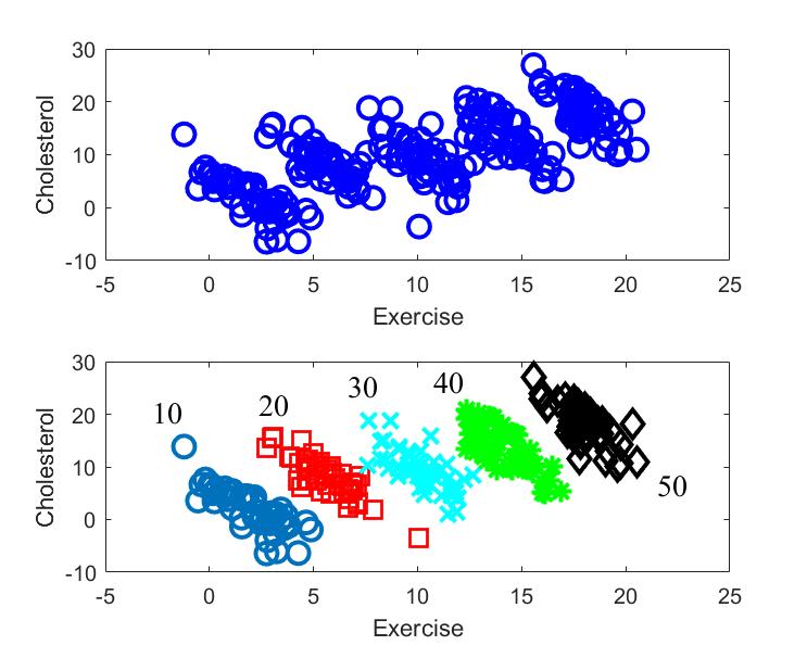
Figure 2.10: Illustration of Simpson’s paradox [Pearl].

The way out of this conundrum is to leverage prior information we have about the problem domain. In fact, we can explain away this spurious correlation by including another measurable variable in the model, namely age. To see this, consider the same data, now redrawn by highlighting the age of the individual corresponding to each data point. The resulting plot, seen in Fig. 2.10 (bottom), reveals that older people — within the observed bracket — tend to have a higher cholesterol as well as to exercise more. Therefore, age is a common cause of both exercise and cholesterol levels. In order to capture the causality relationship between the latter variables, we hence need to adjust for age. Doing this requires to consider the trend within each age separately, recovering the expected conclusion that exercising is useful to lower one’s cholesterol.

We conclude that in this example the correlation between $x$ and $t$, while useful for prediction, should not be acted upon for decision making. When assessing the causal relationship between $x$ and $t$, we should first understand which other variables may explain the observations and then discount any spurious correlations.

This discussion reveals an important limitation of most existing machine learning algorithms when it comes to identifying causality relationships, or, more generally, to answering counterfactual queries [Pearl18]. The study of causality can be carried out within the elegant framework of interventions on probabilistic graphical models developed by Pearl [Pearl, Koller, raginsky2011directed]. Other related approaches are covered in [Peters]. More discussion on probabilistic graphical models can be found in Chapter 7.

2.8 Summary

In this chapter, we have reviewed three key learning frameworks, namely frequentist, Bayesian and MDL, within a parametric probabilistic set-up. The frequentist viewpoint postulates the presence of a true unknown distribution for the data, and aims at learning a predictor that generalizes well on unseen data drawn from this distribution. This can be done either by learning a probabilistic model to be plugged into the expression of the optimal predictor or by directly solving the ERM problem over the predictor. The Bayesian approach outputs a predictive distribution that combines prior information with the data by solving the inference problem of computing the posterior distribution over the unseen label. Finally, the MDL method aims at selecting a model that allows the data to be described with the smallest number of bits, hence doing away with the need to define the task of generalizing over unobserved examples.

The chapter has also focused extensively on the key problem of overfitting, demonstrating how the performance of a learning algorithm can be understood in terms of bias and estimation error. In particular, while choosing a hypothesis class is essential in order to enable learning, choosing the “wrong” class constitutes an irrecoverable bias that can make learning impossible. As a real-world example, as reported in [Oneil], including as independent variables in $x$ the ZIP code of an individual seeking credit at a bank may discriminate against immigrants or minorities. Another example of this phenomenon is the famous experiment by B. F. Skinner on pigeons [Shalev].

We conclude this chapter by emphasizing an important fact about the probabilistic models that are used in modern machine learning applications. In frequentist methods, typically at least two (possibly conditional) distributions are involved: the empirical data distribution and the model distribution. The former amounts to the histogram of the data which, by the law of large numbers, tends to the real distribution when the number of data points goes to infinity; while the latter is parametrized and is subject to optimization. For this reason, divergence metrics between the two distributions play an important role in the development of learning algorithms. We will see in the rest of the monograph that other frequentist methods may involve a single distribution rather than two, as discussed in Sec. 6.6, or an additional, so called variational, distribution, as covered in Sec. 6.3 and Chapter 8.

In contrast, Bayesian methods posit a single coherent distribution over the data and the parameters, and frame the learning problem as one of inference of unobserved variables. As we will discuss in Chapter 8, variational Bayesian methods also introduce an additional variational distribution and are a building block for frequentist learning in the presence of unobserved variables.

The running example in this chapter has been one of linear regression for a Gaussian model. The next chapter provides the necessary tools to construct and learn more general probabilistic models.

Chapter 3 Probabilistic Models for Learning

In the previous chapter, we have introduced the frequentist, Bayesian, and MDL learning frameworks. As we have seen, parametric probabilistic models play a key role for all three of them. The linear regression example considered in the previous chapter was limited to a simple linear Gaussian model, which is insufficient to capture the range of learning problems that are encountered in practice. For instance, scenarios of interest may encompass discrete variables or non-negative quantities. In this chapter, we introduce a family of probabilistic models, known as the exponential family, whose members are used as components in many of the most common probabilistic models and learning algorithms. The treatment here will be leveraged in the rest of the monograph in order to provide the necessary mathematical background. Throughout this chapter, we will specifically emphasize the common properties of the models in the exponential family, which will prove useful for deriving learning algorithms in the following chapters.

3.1 Preliminaries

We start with a brief review of some definitions that will be used throughout the chapter and elsewhere in the monograph (see [Boyd] for more details). Readers with a background in convex analysis and calculus may just review the concept of sufficient statistic in the last paragraph.

First, we define a convex set as a subset of $\mathbb{R}^{D}$, for some $D$, that contains all segments between any two points in the set. Geometrically, convex sets hence cannot have “indentations”. Function $f(x)$ is convex if its domain is a convex set and if it satisfies the inequality $f(\lambda x+(1-\lambda)y)\leq\lambda f(x)+(1-\lambda)f(y)$ for all $x$ and $y$ in its domain and for all $0\leq\lambda\leq 1$. Geometrically, this condition says that the function is “$\cup$”-shaped: the curve defining the function cannot lie above the segment obtained by connecting any two points on the curve. A function is strictly convex if the inequality above is strict except for $\lambda=0$ or $\lambda=1$ when $x\neq y$. A concave, or strictly concave, function is defined by reversing the inequality above – it is hence “$\cap$”-shaped.

The minimization of a convex (“$\cup$”) function over a convex constraint set or the maximization of a concave (“$\cap$”) function over a convex constraint set are known as convex optimization problems. For these problems, there exist powerful analytical and algorithmic tools to obtain globally optimal solutions [Boyd].

We also introduce two useful concepts from calculus. The gradient of a differentiable function $f(x)$ with $x=[x_{1}\cdots x_{D}]^{T}\in\mathbb{R}^{D}$ is defined as the $D\times 1$ vector $\nabla f(x)=[\partial f(x)/\partial x_{1}\cdots\partial f(x)/\partial x_{D}]^{T}$ containing all partial derivatives. At any point $x$ in the domain of the function, the gradient is a vector that points to the direction of locally maximal increase of the function. The Hessian $\nabla^{2}f(x)$ is the $D\times D$ matrix with ($i,j$) element given by the second-order derivative $\partial^{2}f(x)/\partial x_{i}\partial x_{j}$. It captures the local curvature of the function.

Finally, we define the concept of sufficient statistic. Consider a rv $\mathrm{x}\sim p(x|\theta)$, whose distribution depends on some parameter $\theta$. A function $f(x)$ is a sufficient statistic for the estimate of $\theta$ if the likelihood $p(x|\theta)$ of the parameters $\theta$ depends on $x$ only through the function $f(x)$. As an example, for a rv $\mathrm{x}\sim\mathcal{N}(0,\sigma^{2})$, the function $f(x)=x^{2}$ can be easily seen to be sufficient for the estimate of the variance $\sigma^{2}.$

3.2 The Exponential Family

In this section, we introduce the exponential family of parametric probabilistic models. As it will be discussed, this family includes as special cases most of the distributions typically assumed when solving machine learning problems. For example, it includes Gaussian, Laplace, Gamma, Beta and Dirichlet pdfs, as well as Bernoulli, Categorical, multinomial, and Poisson pmfs. An extensive list can be found in [Wikiexp].

3.2.1 Basic Definitions

The exponential family contains probabilistic models of the form

$$p(x|\eta) =\frac{1}{Z(\eta)}\exp\left(\sum_{k=1}^{K}\eta_{k}u_{k}(x)\right)m(x)$$

$$=\frac{1}{Z(\eta)}\exp\left(\eta^{T}u(x)\right)m(x),$$ (3.1)

where $x$ is a discrete or continuous-valued vector; $\eta=[\eta_{1}\cdots\eta_{K}]^{T}$ is the vector of natural parameters; $u(x)=[u_{1}(x)\cdots u_{K}(x)]^{T}$ is the vector of sufficient statistics, with each sufficient statistic $u_{k}(x)$ being a function of $x$; $m(x)\geq 0$ is the base measure, which is a function of $x$ that is independent of the natural parameter vector $\eta;$ and $Z(\eta)$ is the partition function

$$Z(\eta)=\int\exp\left(\eta^{T}u\left(x\right)\right)m\left(x\right)\mathrm{\textrm{d}}x$$ (3.2)

for continuous rvs and $Z(\eta)=\sum_{x}\exp\left(\eta^{T}u\left(x\right)\right)m\left(x\right)$ for discrete rvs. The sufficient statistic vector $u(x)$ can be seen to be a sufficient statistic for the estimation of the natural parameter vector $\eta$ given $x$.

The partition function normalizes the distribution so that it integrates, or sums, to one. It is also often useful to use the unnormalized distribution

$$\tilde{p}(x|\eta)=\exp\left(\eta^{T}u(x)\right)m(x),$$ (3.3)

since the latter is generally easier to evaluate.

In short, distributions belonging to the exponential family are such that the logarithm of the unnormalized distribution $\tilde{p}(x|\eta)$, which is also known as the energy function, is linear in the natural parameters, i.e.,

$$\ln\tilde{p}(x|\eta)=\eta^{T}u(x)+\ln m\left(x\right).$$ (3.4)

For this reason, models of the form (3.1) are also referred to as log-linear. Including the partition function, the LL of the natural parameters can be written as

$$\ln p(x|\eta)=\eta^{T}u\left(x\right)-A(\eta)+\ln m(x),$$ (3.5)

where

$$A(\eta)=\ln Z(\eta)$$ (3.6)

is the log-partition function.

As per (3.1), a probabilistic model belonging to the exponential family is identified by the set of sufficient statistics $\{u_{k}(x)\}_{k=1}^{K}$, whose order is irrelevant, and by the measure $m(x)$. A specific hypothesis within the model is selected by determining the natural parameter vector $\eta$. The set of feasible values for the natural parameters contains all, and only, the vectors $\eta$ for which the unnormalized distribution $\tilde{p}(x|\eta)$ can be normalized, that is, for which the inequality $A(\eta)<\infty$ holds. We will see below that this set is convex.

Example 3.2.1.

(Gaussian pdf) As a first example, consider the Gaussian pdf

$$\mathcal{N}(x|\nu,\sigma^{2} )=\frac{1}{(2\pi\sigma^{2})^{1/2}}\exp\left(\mathrm{-}\frac{x^{2}}{2\sigma^{2}}+\frac{\nu}{\sigma^{2}}x-\frac{\nu^{2}}{2\sigma^{{}^{2}}}\right).$$

This can be written in the form (3.1) upon identification of the base measure $m(x)=1$ and of the sufficient statistics $u(x)=[x\textrm{ $x^{2}$}]$. Note that, in order to do this, we need to map the parameters $(\nu,\sigma^{2})$ to the natural parameters via the relationship $\eta=[\nu/\sigma^{2}\textrm{$\textrm{ }-1/$$(2$$\sigma^{2}$) }]$. As a result, while the parameters $(\nu,\sigma^{2})$ take all possible allowed values in $\mathbb{R}\times\mathbb{R}^{+}$, the natural parameter vector $\eta$ takes values in the set $\mathbb{R}\times\mathbb{R}^{-}$. Every value $\eta$ in this set corresponds to a valid pdf within the hypothesis class of $\mathcal{N}(x|\nu,\sigma^{2})$ models. Finally, we can compute the log-partition function as

$$A(\eta)=\frac{\nu^{2}}{2\sigma^{2}}+\frac{1}{2}\text{ln}(2\pi\sigma^{2})=-\frac{\eta_{1}^{2}}{4\eta_{2}}-\frac{1}{2}\text{ln}\left(-\left(\frac{2\eta_{2}}{2\pi}\right)\right).$$ (3.7)

In order to ensure identifiability of the natural parameters, the sufficient statistics $\{u_{k}(x)\}_{k=1}^{K}$ need to be linearly independent. This means that no sufficient statistic $u_{k}(x)$ should be computable, for all $x$, as a linear combination of other sufficient statistics $u_{k^{\prime}}(x)$ with $k^{\prime}\neq k$. For example, this is the case for the vector $u(x)=[x\textrm{ $x^{2}$}]$ of sufficient statistics for the Gaussian distribution. This condition is referred to as minimal representation [Wainwright]. Unless stated otherwise, we will assume in the following that the exponential family under study is minimal. Furthermore, we will assume the technical condition that the set of feasible values for $\eta$ is also open (that is, it excludes its boundary), which yields a regular exponential family.

3.2.2 Natural Parameters, Mean Parameters and Convexity

As suggested by the example above, once the sufficient statistics and the base measure are fixed, a specific hypothesis – pdf or pmf – can be identified by either specifying the vector $\eta$ of natural parameters or the vector $\mu$ of mean parameters. The latter is defined as the expectation of the vector of sufficient statistics

$$\mu=\mathrm{E}_{\mathrm{x}\sim p(x|\eta)}[u(\mathrm{x})].$$ (3.8)

For the preceding example, we have the mean parameter vector $\mu=[\textrm{E}[\mathrm{x}]=\nu,\textrm{ E$[\mathrm{x}^{2}]=\sigma^{2}+\nu^{2}$}]^{T}$. We can therefore use the notation $p(x|\mu)$ as well as $p(x|\eta)$ to describe a model in the exponential family. As we will see below, the availability of these two parametrizations implies that learning can be done on either sets of variables.

A key property of the exponential family is that the mapping between natural parameters and mean parameters is given by the gradient of the log-partition function. Specifically, it can be verified that the partial derivative of the log-partition function equals the mean of the corresponding sufficient statistic

$$\frac{\partial A(\eta)}{\partial\eta_{k}}=\textrm{E}_{\mathrm{x}\sim p(x|\eta)}\left[u_{k}\left(\mathrm{x}\right)\right]=\mu_{k},$$ (3.9)

or, in vector form,

$$\nabla_{\eta}A(\eta)=\textrm{E}_{\mathrm{x}\sim p(x|\eta)}\left[u\left(\mathrm{x}\right)\right]=\mu.$$ (3.10)

Although we will not be making use of this result here, the Hessian $\nabla_{\eta}^{2}A(\eta)$ of the log-partition function can be similarly seen to equal the covariance matrix of the sufficient statistics. It is also equal to the Fisher information matrix for the natural parameters [Duchicourse].

The log-partition function $A(\eta)$ in (3.6) is strictly convex in $\eta$, as it follows from the fact that it is a log-sum-exp function composed with an affine function [Boyd]. This property has the following important consequences. First, the set of feasible values for the natural parameters is a convex set [Boyd]. Note that this is generally not the case for the corresponding set of feasible values for the mean parameters. Second, the mapping (3.10) between natural parameters $\eta$ and mean parameters $\mu$ is invertible (see, e.g., [azoury2001relative]).

Third, the LL function $\ln p(x|\eta)$ in (3.5) is a concave function of $\eta$. As further discussed below, the ML problem hence amounts to maximization of a convex optimization problem.

3.2.3 Bernoulli Model

Due to its importance for binary classification problems, we detail here the Bernoulli model. We also introduce the important logistic sigmoid function.

The Bernoulli distribution for a binary rv $\mathrm{x}\in\{0,1\}$ is given as

$$\textrm{Bern}(x|\mu)=\mu^{x}\left(1-\mu\right)^{1-x},$$ (3.11)

with $\mu=\textrm{E}_{\mathrm{x}\sim\textrm{Bern}(x|\mu)}\left[\mathrm{x}\right]=\textrm{Pr}[\mathrm{x}=1]$. Since we can write the LL function as

$$\textrm{ln}\left(\textrm{Bern}(x|\mu)\right)=\textrm{ln$\left(\frac{\mu}{1-\mu}\right)x$}+\textrm{ln}\left(1-\mu\right),$$ (3.12)

the sufficient statistic defining the Bernoulli model is $u(x)=x$ and the measure function is $m(x)=1$. The mapping between the natural parameter $\eta$ and the mean parameter $\mu$ is given as

$$\eta=\text{ln}\left(\frac{\mu}{1-\mu}\right),$$ (3.13)

that is, the natural parameter is the LLR $\eta=\textrm{ln}(\textrm{Bern}(1|\mu)/\textrm{Bern}(0|\mu))$. Function (3.13) is also known as the logit function. The corresponding set of feasible values is hence $\mathbb{R}$.

The inverse mapping is instead given by the logistic sigmoid function

$$\mu=\sigma(\eta)=\frac{1}{1+e^{-\eta}}.$$ (3.14)

The sigmoid function converts a real number into the interval $[0,1]$ via an S-shape that associates values less than 0.5 to negative values of the argument and larger values to positive numbers. Finally, the log-partition function is given by the convex function of the natural parameters

$$A(\eta)=-\text{ln}(1-\mu)=\text{ln}(1+e^{\eta}).$$ (3.15)

Note that the relationship (3.10) is easily verified.

3.2.4 Categorical or Multinoulli Model

For its role in multi-class classification, we introduce here in some detail the Categorical or Multinoulli distribution, along with the one-hot encoding of categorical variables and the soft-max function.

The Categorical model applies to discrete variables taking $C$ values, here labeled without loss of generality as $\{0,1,...,C-1\}.$ Note that setting $C=2$ recovers the Bernoulli distribution. Pmfs in this model are given as

$$\textrm{Cat}(x|\mu)=\prod_{k=1}^{C-1}\mu_{k}^{1\left(x=k\right)}\times\mu_{0}^{1-\sum_{k=1}^{C-1}1(x=k)},$$ (3.16)

where we have defined $\mu_{k}=\textrm{Pr}\left[\mathrm{x}=k\right]$ for $k=1,\ldots,C-1$ and $\mu_{0}=1-\sum_{k=1}^{C-1}\mu_{k}=\textrm{Pr}\left[\mathrm{x}=0\right]$. The LL function is given as

$$\textrm{ln}\left(\textrm{Cat}(x|\mu)\right)=\sum_{k=1}^{C-1}1\left(x=k\right)\textrm{ln}\frac{\mu_{k}}{\mu_{0}}\textrm{+ln}\mu_{0}.$$ (3.17)

This demonstrates that the categorical model is in the exponential family, with sufficient statistics vector $u(x)=[1(x=1)\cdots 1(x=C-1)]^{T}$ and measure function $m(x)=1$. Furthermore, the mean parameters $\mu=[\mu_{1}\cdots\mu_{C-1}]^{T}$ are related to the natural parameter vector $\eta=[\eta_{1}\cdots\eta_{C-1}]^{T}$ by the mapping

$$\eta_{k}=\ln\left(\frac{\mu_{k}}{1-\sum_{j=1}^{C-1}\mu_{j}}\right),$$ (3.18)

which again takes the form of an LLR. The inverse mapping is given by

$$\mu=\begin{bmatrix}\frac{e^{\eta_{1}}}{1+\sum_{k=1}^{C-1}e^{\eta_{k}}}\\ \vdots\\ \frac{e^{\eta_{C-1}}}{1+\sum_{k=1}^{C-1}e^{\eta_{k}}}\end{bmatrix}.$$ (3.19)

The parametrization given here is minimal, since the sufficient statistics $u(x)$ are linearly independent. An overcomplete representation would instead include in the vector of sufficient statistics also the function $1(x=0)$. In this case, the resulting vector of sufficient statistics

$$u(x)=\begin{bmatrix}1(x=0)\\ \vdots\\ 1(x=C-1)\end{bmatrix}$$ (3.20)

is known as one-hot encoding of the categorical variable, since only one entry equals 1 while the others are zero. Furthermore, with this encoding, the mapping between the natural parameters and the mean parameters $\mu=[\mu_{0}\cdots\mu_{C-1}]^{T}$ can be expressed in terms of the softmax function

$$\mu=\textrm{softmax($\eta$)=}\begin{bmatrix}\frac{e^{\eta_{0}}}{\sum_{k=0}^{C-1}e^{\eta_{k}}}\\ \vdots\\ \frac{e^{\eta_{C-1}}}{\sum_{k=0}^{C-1}e^{\eta_{k}}}\end{bmatrix}.$$ (3.21)

The softmax function $\textrm{softmax}(\eta)$ converts a vector of “scores” $\eta$ into a probability vector. Furthermore, the function has the property that, as $c$ grows to infinity, softmax($c\eta$) tends to a vector with all zero entries except for the position corresponding to the maximum value $\eta_{k}$ (assuming that it is unique). This justifies its name.

3.3 Frequentist Learning

In this section, we provide general results concerning ML and MAP learning when the probabilistic model belongs to the exponential family. As seen in the previous chapter, with ML and MAP, one postulates that the $N$ available data points $x_{\mathcal{D}}=\{x_{1},\ldots,x_{N}\}$ are i.i.d. realizations from the probabilistic model $p(x|\eta)$ as

$$\mathrm{x}_{n}\underset{\textrm{i.i.d.}}{\sim}p(x|\mathbf{\eta}),\textrm{ $n=1,...,N$}.$$ (3.22)

This data is used to estimate the natural parameters $\mathbf{\eta}$, or the corresponding mean parameters $\mu$.

Using (3.5), the LL of the natural parameter vector given the observation $x_{\mathcal{D}}$ can be written as

$$\text{ln}p(x_{\mathcal{D}}|\eta) =\sum_{n=1}^{N}\text{ln}p(x_{n}|\eta)$$

$$=-NA(\eta)+\eta^{T}\sum_{n=1}^{N}u(x_{n})+\sum_{n=1}^{N}\textrm{ln$m$}(x_{n}).$$ (3.23)

Therefore, neglecting terms independent of $\eta$, we can write

$$\text{ln}p(x_{\mathcal{D}}|\eta) =-NA(\eta)+\eta^{T}u(x_{\mathcal{D}}),$$ (3.24)

where we have defined the cumulative sufficient statistics

$$u_{k}(x_{\mathcal{D}})=\sum_{n=1}^{N}u_{k}(x_{n}),\textrm{ }k=1,...,K,$$ (3.25)

and the vector $u(x_{\mathcal{D}})=[u_{1}(x_{\mathcal{D}})\cdots u_{K}(x_{\mathcal{D}})]^{T}$.

A first important observation is that the LL function only depends on the $K$ statistics $u_{k}(x_{\mathcal{D}})$, $k=1,...,K$. Therefore, the vector $u(x_{\mathcal{D}})$ is a sufficient statistic for the estimate of $\eta$ given the observation $x_{\mathcal{D}}$. Importantly, vector $u(x_{\mathcal{D}})$ is of size $K$, and hence it does not grow with the size $N$ of the data set. In fact, the exponential family turns out to be unique in this respect: Informally, among all distributions whose support does not depend on the parameters, only distributions in the exponential family have sufficient statistics whose number does not grow with the number $N$ of observations (Koopman-Pitman-Darmois theorem) [angelino2016patterns].

Gradient of the LL function. A key result that proves very useful in deriving learning algorithms is the expression of the gradient of the LL (3.24) with respect to the natural parameters. To start, the partial derivative with respect to $\eta_{k}$ can be written as

$$\frac{\partial\textrm{ln}p(x_{\mathcal{D}}|\eta)}{\partial\eta_{k}}=u_{k}(x_{\mathcal{D}})-N\frac{\partial A(\eta)}{\partial\eta_{k}}.$$ (3.26)

Using (3.9) and (3.10), this implies that we have

$$\frac{1}{N}\frac{\partial\textrm{ln}p(x_{\mathcal{D}}|\eta)}{\partial\eta_{k}}=\frac{1}{N}u_{k}(x_{\mathcal{D}})-\mu_{k},$$ (3.27)

and for the gradient

$$\frac{1}{N}\nabla_{\eta}\textrm{ln}p(x_{\mathcal{D}}|\eta) =\frac{1}{N}u(x_{\mathcal{D}})-\mu$$

$$=\frac{1}{N}\sum_{n=1}^{N}u(x_{n})-\mu.$$ (3.28)

The gradient (3.28) is hence given by the difference between the empirical average $N^{-1}\sum_{n=1}^{N}u(x_{n})$ of the sufficient statistics given the data $x_{\,\mathcal{D}}$ and the ensemble average $\mu$.

The following observation is instrumental in interpreting algorithms based on gradient ascent or descent for exponential families. The normalized gradient of the LL (3.28) has two components: (i) the “positive” component $u(x_{\mathcal{D}})/N$ points in a direction of the natural parameter space that maximizes the unnormalized distribution $\ln\tilde{p}(x_{\mathcal{D}}|\eta)=\eta^{T}u(x_{\mathcal{D}})+\sum_{n=1}^{N}\ln m(x_{n})$, hence maximizing the “fitness” of the model to the observed data $x_{\mathcal{D}}$; while (ii) the “negative” component $-\mu=-\nabla_{\eta}A(\eta)$ points in a direction that minimizes the partition function, thus minimizing the “fitness” of the model to the unobserved data. The tension between these two components is resolved when the empirical expectation of the sufficient statistics equals that under the model, as discussed below.

ML Learning. Due to concavity of the LL function, or equivalently convexity of the NLL, and assuming the regularity of the distribution, the ML estimate $\eta$_ML is obtained by imposing the optimality condition

$$\nabla_{\eta}\text{ln}p(x_{\mathcal{D}}|\eta)=0,$$ (3.29)

which gives

$$\mu_{\text{$ML$}}=\frac{1}{N}\sum_{n=1}^{N}u(x_{n}).$$ (3.30)

In words, the ML estimate of the mean parameters is obtained by matching the ensemble averages obtained under the model to the empirical averages observed from the data. This procedure is known as moment matching. Note that, from (3.30), if needed, we can also compute the ML estimate $\eta_{\text{$ML$}}$ using the mapping between the two sets of parameters.

From (3.30), we can infer that the ML estimate is consistent: if the data is generated from a distribution $p(x|\eta^{*})$ within the assumed family, the ML estimate will tend to it with probability one as $N$ grows to infinity by the strong law of large numbers [lehmann2006theory]. However, for finite $N$, ML may suffer from overfitting, as we will see next.

Example 3.3.1.

(Gaussian pdf). The ML estimates of the parameters $(\mu,\,\sigma^{2}$) for the Gaussian model are given as

$$\mu_{\text{$ML$}} =\frac{1}{N}\sum_{n=1}^{N}x_{n}$$ (3.31)

$$\sigma_{\text{$ML$}}^{2} =\frac{1}{N}\sum_{n=1}^{N}x_{n}^{2}-\mu_{\text{$ML$}}^{2}.$$ (3.32)

For the Bernoulli model, we have the ML estimate of the mean parameter $\mu=\textrm{Pr}\left[\mathrm{x}=1\right]$

$$\mu_{\text{$ML$}}=\frac{1}{N}\sum_{n=1}^{N}x_{n}=\frac{N[1]}{N},$$ (3.33)

where $N\left[k\right]$ measures the number of observations equal to $k$, i.e.,

$$N[k]=|\{n:\;x_{n}=k\}|.$$

Note that $N[1]$ has a binomial distribution. For the Categorical model, we can similarly write the ML estimate of the mean parameters $\mu_{k}=\textrm{Pr}\left[\mathrm{x}=k\right]$ as

$$\mu_{k,\text{$ML$}} =\frac{1}{N}\sum_{n=1}^{N}1(x_{n}=k)=\frac{N[k]}{N}.$$ (3.34)

The vector $[N[0],...,N[C-1]]^{T}$ has a multinomial distribution.

To illustrate the problem of overfitting, consider the categorical model. As per (3.34), if no instance of the data equal to some value $k$ is observed, i.e., if $N[k]=0$, ML assigns a zero probability to the event $\mathrm{x}=k$. In mathematical terms, if $N[k]=0,$ the ML estimate of the probability of the event $\mathrm{x}=k$ is zero, that is, $\mu_{k,\text{$ML$}}=0$. So, ML gives zero probability to any previously unobserved event. The problem, which is an instance of overfitting, is known as the black swan paradox or zero-count problem: For the European explorers of the 17th century – or at least for those of them adhering to the ML principle – the black swans in the Americas could not exist! [Murphy]

MAP Learning. A MAP solution can be in principle derived by including in the optimality condition (3.29) the gradient of the prior distribution. We will instead solve the MAP problem in the next section by computing the mode of the posterior distribution of the parameters.

3.4 Bayesian Learning

As we discussed in the previous chapter, the Bayesian viewpoint is to treat all variables as jointly distributed, including the model parameters $\mu$ and the new, unobserved value $\mathrm{x}.$ The joint distribution is given as

$$p(x_{\mathcal{D}},\mu,x|\alpha)=\underbrace{p(\mu|\alpha)}_{\text{a priori distribution}}\underbrace{p(x_{\mathcal{D}}|\mu)}_{\text{ likelihood}}\underbrace{p(x|\mu)}_{\text{ distribution of new data}},$$ (3.35)

where $\alpha$ represents the vector of hyperparameters defining the prior distribution. The problem of inferring the unobserved value $\mathrm{x}$ is solved by evaluating the predictive distribution

$$p(x|x_{\mathcal{D}},\alpha)=\int p(\mu|x_{\mathcal{D}},\alpha)p(x|\mu)\text{$d$}\mu.$$ (3.36)

This distribution accounts for the weighted average of the contributions from all values of the parameter vector $\mu$ according to the posterior distribution $p(\mu|x_{\mathcal{D}},\alpha).$ Note that, for clarity, we left indicated the dependence on the hyperparameters $\alpha.$ Using Bayes’ theorem, the posterior of the parameter vector can be written as

$$p(\mu|x_{\mathcal{D}},\alpha)=\frac{p(\mu|\alpha)p(x_{\mathcal{D}}|\mu)}{p(x_{\mathcal{D}}|\alpha)}\propto p(\mu|\alpha)p(x_{\mathcal{D}}|\mu).$$ (3.37)

As discussed in Chapter 2, this relationship highlights the dependence of the posterior on both the prior distribution and the likelihood $p(x_{\mathcal{D}}|\mu)$. We also note the the denominator in (3.37) is the marginal likelihood.

Prior distribution. The first issue we should address is the choice of the prior distribution. There are two main approaches: 1) Conjugate prior: choose the prior $p(\mu|\alpha)$, so that posterior $p(\mu|x_{\mathcal{D}},\alpha)$ has the same distribution as the prior $p(\mu|\alpha)$ but with generally different parameters; 2) Non-informative prior: choose the prior that is the least informative given the observed data [Bishop, pp. 117-120]. Here, we will work with conjugate priors, which are more commonly adopted in applications. In fact, a key advantage of models in the exponential family is that they all admit conjugate priors, and the conjugate priors are also members of the exponential family.

Rather than providing a general discussion, which may be of limited practical use, we proceed by means of representative examples. A table of models with corresponding prior distributions can be found in [Wikiconj].

3.4.1 Beta-Bernoulli Model

The Beta-Bernoulli model is suitable to study binary data. Conditioned on the parameter $\mu=\textrm{Pr}\left[\mathrm{x}=1\right]$, the pmf of the $N$ i.i.d. available observations $x_{\mathcal{D}}$ with $x_{n}\in\{0,1\}$ is given as

$$p(x_{\mathcal{D}}|\mu)=\prod_{n=1}^{N}\textrm{Bern}(x_{n}|\mu)=\mu^{N[1]}(1-\mu)^{N[0]}.$$ (3.38)

As seen, a conjugate prior should be such that the posterior (3.37) has the same distribution of the prior but with different parameters. For the likelihood (3.38), the conjugate prior is the Beta distribution, which is defined as

$$\begin{split}p(\mu|a,b)&=\text{Beta}(\mu|a,b)\propto\mu^{a-1}(1-\mu)^{b-1},\end{split}$$ (3.39)

where $a$ and $b$ are hyperparameters and the normalization constant is not made explicit in order to simplify the notation. It is worth emphasizing that (3.39) is a probability distribution on a probability $\mu$. Plots of the beta pdf for different values of $a,b\geq 1$ can be found in Fig. 3.1.

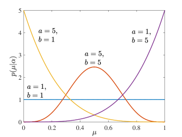
Figure 3.1: Beta distribution with different values of the hyperparameters $a,b\geq 1.$

Average and mode of the Beta pdf can be evaluated as

$$\text{E}_{\mu\sim\text{Beta}(\mu|a,b)}[\mu] =\frac{a}{a+b}$$ (3.40)

$$\text{mode}_{\text{$\mu\sim$Beta}(\mu|a,b)} [\mu]=\frac{a-1}{a+b-2}\quad,$$ (3.41)

where the mode expression is only valid when $a,b>1$ (when this condition is not met, the distribution is multi-modal, see Fig. 3.1). The mean (3.39) suggests that the hyperparameters $a$ and $b$ can be interpreted as the number of observations that are expected to equal “1” and “0”, respectively, out of a total number of $a+b$ measurements, based on prior information alone. More fittingly, as we shall see next, we can think of these a priori observations as “virtual” measurements, also known as pseudo-counts, that should be used alongside the actual measurements $x_{\mathcal{D}}$ during learning.

We can now compute the posterior distribution of the parameter vector using (3.37) as

$$p(\mu|x_{\mathcal{D}},a,b) \propto\text{Beta}\left(\mu\left|a+N[1],b+N[0]\right.\right)$$

$$=\mu^{N[1]+a-1}(1-\mu)^{N[0]+b-1}.$$ (3.42)

This confirms that the posterior distribution is indeed a Beta pdf, as dictated by the choice of a Beta conjugate prior. Furthermore, the posterior Beta distribution has parameters $a+N[1]$ and $b+N[0]$. This is consistent with the interpretation given above: the total number of effective observations equal to “1” and “0” are $a+N[1]$ and $b+N[0]$, respectively. As anticipated, the MAP estimate of $\mu$ can be obtained by taking the mode of the posterior (3.37), yielding

$$\mu_{\text{$MAP$}}=\frac{a+N[1]-1}{a+b+N-2}.$$ (3.43)

As we discussed in the previous chapter, we have the limit $\mu_{\text{$MAP$}}\rightarrow\mu_{ML}$ for $N\rightarrow\infty$.

Back to the Bayesian viewpoint, the predictive distribution (3.36) is given as

$$p(x=1|x_{\mathcal{D}},a,b) =\int p(\mu|x_{\mathcal{D}},a,b)p(x=1|\mu)\text{$d$}\mu$$

$$=\text{E}_{\mu\sim p(\mu|x_{\mathcal{D}},a,b)}[\mu]=\frac{N[1]+a}{N+a+b}$$ (3.44)

where we have used the expression (3.40) for the mean of a Beta rv. We observe that, if $N$ is small, the predictive probability is approximately equal to the mean of the prior, i.e., $p(x=1|x_{\mathcal{D}},a,b)\approx a/(a+b)$; while, if $N$ is large, as we have seen in the previous chapter, the predictive probability tends to the ML solution, i.e., $p(x=1|x_{\mathcal{D}},a,b)\approx N[1]/N.$

As an example of a non-conjugate prior, one could choose the distribution of the natural parameter $\eta$, or equivalently of the logit function (3.13) of $\mu$, as Gaussian [lunn2012bugs].

The following example illustrates the potential advantages, already discussed in Chapter 2, of the Bayesian approach in avoiding overfitting. Note that MAP would also yield similar results in this example.

Example 3.4.1.

(Predicting online reviews) On an online shopping platform, there are two sellers offering a product at the same price. The first has 30 positive reviews and 0 negative reviews, while the second has 90 positive reviews and 10 negative reviews. Which one to choose? To tackle this problem, we can learn a Beta-Bernoulli model to predict whether the next review will be positive or not. We can compute the probability that the next review is positive via the predictive distribution (3.44). The result is shown in Fig. 3.2: While the first seller has a 100% positive rate, as opposed to the 90% rate of the first seller, we prefer to choose the first seller unless the prior distribution is weak, which translates here into the condition $a=b\lesssim 3$.

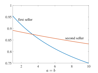
Figure 3.2: Probability that the next review is positive using the predictive distribution (3.44) for Example 3.3.

3.4.2 Dirichlet-Categorical Model

The Dirichlet-Categorical model generalizes the Beta-Bernoulli model to the case of discrete observations that can take any number $C$ of values. The treatment follows along the same lines as for the Beta-Bernoulli model, and hence we provide only a brief discussion. The likelihood function can be written as

$$p(x_{\mathcal{D}}|\mu)=\prod_{k=0}^{C-1}\mu_{k}^{N[k]}.$$ (3.45)

The conjugate prior is the Dirichlet distribution, a generalization of the Beta distribution:

$$\begin{split}p(\mu|\alpha)&=\text{Dir}(\mu|\alpha)\propto\prod_{k=0}^{C-1}\mu_{k}^{\alpha_{k}-1},\end{split}$$ (3.46)

where $\alpha_{k}$ is the hyperparameter representing the number of “prior” observations equal to $k$. Note that the Dirichlet distribution is a joint pdf for the entries of the mean vector $\mu$. Mean and mode vectors for the Dirichlet distribution are given as

$$\text{E}_{\mu\sim\text{Dir}(\mu|\alpha)}[\mu] =\frac{\alpha}{\sum_{j=0}^{C-1}\alpha_{j}}$$ (3.47)

mode$${}_{\text{$\mu\sim$Dir}(\mu|\alpha)} [\mu]=\frac{\alpha-1}{\sum_{j=0}^{C-1}\alpha_{j}-C}.$$ (3.48)

The posterior of the parameters is the Dirichlet distribution

$$p(\mu|x_{\mathcal{D}},\alpha)\propto\prod_{k=0}^{C-1}\mu_{k}^{N[k]+\alpha_{k}-1}=\text{Dir}(\mu|\alpha+N),$$ (3.49)

in which we can again interpret $\alpha_{k}+N[k]$ as the effective number of observations equal to $k$. From this distribution, we can obtain the MAP estimate as the mode. Finally, the Bayesian predictive distribution is

$$p(x=k|x_{\mathcal{D}},\alpha)=\frac{N[k]+\alpha_{k}}{N+\sum_{j=0}^{C-1}\alpha_{j}}.$$ (3.50)

One can check that the behavior in the two regimes of small and large $N$ is consistent with the discussion on the Beta-Bernoulli model.

3.4.3 Gaussian-Gaussian Model

As a last example, we consider continuous observations that are assumed to have a Gaussian distribution $\mathcal{N}(\mu,\sigma^{2})$ with unknown mean $\mu$ but known variance $\sigma^{2}$. The likelihood function is hence $p(x_{\mathcal{D}}|\mu)=\prod_{n=1}^{N}\mathcal{N}(x_{n}|\mu,\sigma^{2})$. The conjugate prior is also Gaussian, namely $p(\mu|\mu_{0},\sigma_{0}^{2})=\mathcal{N}(\mu|\mu_{0},\sigma_{0}^{2}),$ with hyperparameters ($\mu_{0},\sigma_{0}^{2}$). The posterior $p(\mu|x_{\mathcal{D}\,},\mu_{0},\sigma_{0}^{2})=\mathcal{N}(\mu|\mu_{N},\sigma_{N}^{2})$ is hence Gaussian, with mean and variance satisfying

$$\mu_{N} =\frac{\sigma^{2}/N}{\sigma_{0}^{2}+\sigma^{2}/N}\mu_{0}+\frac{\sigma_{0}^{2}}{\sigma_{0}^{2}+\sigma^{2}/N}\mu_{\text{$ML$}}$$ (3.51)

$$\frac{1}{\sigma_{N}^{2}} =\frac{1}{\sigma_{0}^{2}}+\frac{N}{\sigma^{2}},$$ (3.52)

where we recall that the ML estimate is $\mu_{ML}=\sum_{n=1}^{N}x_{n}/N.$ Note that, since mean and mode are equal for the Gaussian distribution, the mean $\mu_{N}$ is also the MAP estimate $\mu_{MAP}$ of $\mu$. Finally, the predictive distribution is also Gaussian and given as $p(x|x_{\mathcal{D}},\mu_{0},\sigma_{0}^{2})=\mathcal{N}(x|\mu_{\text{$N$}},\sigma^{2}+\sigma_{N}^{2}$). Once again, as $N$ grows large, the predictive distribution tends to that returned by the ML approach, namely $\mathcal{N}(x|\mu_{ML},\sigma^{2})$.

Fig. 3.3 illustrates the relationship among ML, MAP and Bayesian solutions for the Gaussian-Gaussian model. In all the panels, the dotted line represents the prior distribution, which is characterized by the parameters ($\mu_{0}=1$, $\sigma_{0}^{2}=3$), and the dashed line is the true distribution of the data, which is assumed to be Gaussian with parameters ($\mu=0,$ $\sigma^{2}=1$), hence belonging to the assumed model. Each subfigure plots a realization of $N$ observations (circles), along with the ML solution (diamond) and the MAP estimate (star). The solid lines represent the Bayesian predictive distribution.

As $N$ increases, we observe the following, already discussed, phenomena: (i) the ML estimate $\mu_{ML}$ consistently estimates the true value $\mu=0$; (ii) the MAP estimate $\mu_{MAP}$ tends to the ML estimate $\mu_{ML}$; and (iii) the Bayesian predictive distribution tends to the ML predictive distribution, which in turn coincides with the true distribution due to (i).

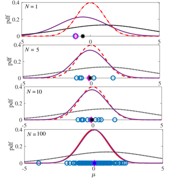
Figure 3.3: Gaussian-Gaussian model: prior distribution $\mathcal{N}$($x|\mu_{0}=1$,$\sigma_{0}^{2}=3$) (dotted), true distribution $\mathcal{N}$($x|\mu=0,$$\sigma^{2}=1$) (dashed), $N$ observations (circles), ML solution (diamond), the MAP estimate (star), and Bayesian predictive distribution (solid line).

3.5 Supervised Learning via Generalized Linear Models (GLM)

Distributions in the exponential family are not directly suitable to serve as discriminative probabilistic models to be used in supervised learning tasks. In this section, we introduce Generalized Linear Models (GLMs), which are popular probabilistic discriminative models that build on members of the exponential family.

To elaborate, let us denote as exponential($\cdot|\eta$) a probabilistic model in the exponential family, that is, a model of the form $(\ref{eq:exponential family}$) with natural parameters $\eta$. We also write exponential($\cdot|\mu$) for a probabilistic model in the exponential family with mean parameters $\mu$.

Using the notation adopted in the previous chapter, in its most common form, a GLM defines the probability of a target variable $\mathrm{t}$ as

$$p(t|x,W)=\textrm{exponential(}t|\eta=Wx),$$ (3.53)

where we recall that $x$ is the vector of explanatory variables, and $W$ here denotes a matrix of learnable weights of suitable dimensions. According to (3.53), GLMs posit that the response variable $\mathrm{t}$ has a conditional distribution from the exponential family, with natural parameter vector $\eta=Wx$ given by a linear function of the given explanatory variables $x$ with weights $W$. More generally, we may have the parametrization

$$p(t|x,W)=\textrm{exponential(}t|\eta=W\phi(x))$$ (3.54)

for some feature vector $\phi(\cdot)$ obtained as a function of the input variables $x$ (see next chapter).

While being the most common, the definition (3.54) is still not the most general for GLMs. More broadly, GLMs can be interpreted as a generalization of the linear model considered in the previous chapter, whereby the mean parameters are defined as a linear function of a feature vector. This viewpoint, described next, may also provide a more intuitive understanding of the modelling assumptions made by GLMs.

Recall that, in the recurring example of Chapter 2, the target variable was modelled as Gaussian distributed with mean given by a linear function of the covariates $x$. Extending the example, GLMs posit the conditional distribution

$$p(t|x,W)=\textrm{exponential(}t|\mu=g(W\phi(x))),$$ (3.55)

where the mean parameter vector is parametrized as a function of the feature vector $\phi(x)$ through a generally non-linear vector function $g(\cdot)$ of suitable dimensions. In words, GLM assume that the target variable is a “noisy” measure of the mean $\mu=g(W\phi(x)).$

When the function $g(\cdot)$ is selected as the gradient of the partition function of the selected model, e.g., $g(\cdot)=\nabla_{\eta}A(\cdot),$ then, by (3.10), we obtain the GLM (3.54). This choice for $g(\cdot)$ is typical, and is referred to as the (inverse of the) canonical link function. For instance, the linear regression model $p(t|x,w)=\mathcal{N}(t|w^{T}\phi(x),\sigma^{2})$ used in Chapter 2 corresponds to a GLM with canonical link function. Throughout this monograph, when referring to GLMs, we will consider models of the form (3.54), or, equivalently (3.55), with canonical link function. For further generalizations, we refer to [Murphy, Barber].

GLMs, especially in the form (3.54), are widely used. As we will also discuss in the next chapter, learning the parameters of GLMs can be done by means of gradient ascent on the LL using the identity (3.28) and the chain rule of differentiation.

3.6 Maximum Entropy Property^∗

In this more technical section, we review the maximum entropy property of the exponential family. Beside providing a compelling motivation for adopting models in this class, this property also illuminates the relationship between natural and mean parameters.

The key result is the following: The distribution $p(x|\mathbf{\eta})$ in (3.1) obtains the maximum entropy over all distributions $p(x)$ that satisfy the constraints $\textrm{E}_{\mathrm{x}\sim p(x)}[u_{k}(\mathrm{x})]=\mu_{k}$ for all $k=1,...,K$. Recall that, as mentioned in Chapter 2 and discussed in more details in Appendix A, the entropy is a measure of randomness of a random variable. Mathematically, the distribution $p(x|\mathbf{\eta})$ solves the optimization problem

$$\underset{p\left(x\right)}{\textrm{max }}H(p)\textrm{ {s.t.}\;E${}_{\mathrm{x}\sim p(x)}\left[u_{k}(\mathrm{x})\right]$=$\mu_{k}$\;{for}\;$k=1,...,K.$}$$ (3.56)

Each natural parameter $\eta_{k}$ turns out to be the optimal Lagrange multiplier associated with the $k$th constraint (see [Duchicourse, Ch. 6-7]).

To see the practical relevance of this result, suppose that the only information available about some data $x$ is given by the means of given functions $u_{k}(x),$ $k=1,...,K$. The probabilistic model (3.1) can then be interpreted as encoding the least additional information about the data, in the sense that it is the “most random” distribution under the given constraints. This observation justifies the adoption of this model by the maximum entropy principle.

Furthermore, the fact that the exponential distribution solves the maximum entropy problem (3.56) illuminates the relationship between mean parameters $\{\mu_{k}\}$ and natural parameters $\{\eta_{k}\}$, as the natural parameter $\eta_{k}$ is the optimal Lagrange multiplier associated with the constraint $E_{\mathrm{x}\sim p(x)}\left[u_{k}(\mathrm{x})\right]=\mu_{k}.$

As another note on the exponential family and information-theoretic metrics, in Appendix B we provide discussion about the computation of the KL divergence between two distributions in the same exponential family but with different parameters.

3.7 Energy-based Models^∗

A generalization of the exponential family is given by probabilistic models of the form

$$p(x|\eta)=\frac{1}{Z(\eta)}\exp\left(-\sum_{c}E_{c}(x_{c}|\eta)\right),$$ (3.57)

where functions $E_{c}(x_{c}|\eta)$ are referred to as energy functions and $Z(\eta)$ is the partition function. Each energy function $E_{c}(x_{c}|\eta)$ generally depends on a subset $x_{c}$ of the variables in vector $x$. If each energy function depends linearly on the parameter vector $\eta$, we recover the exponential family discussed above. However, the energy functions may have a more general non-linear form. An example is the function $E_{c}(x_{c}|\eta)=\ln\left(1+(\eta_{c}^{T}x_{c})^{2}\right)$ corresponding to a Student’s t-distribution model [lecun2006tutorial].

Models in the form (3.57) encode information about the plausibility of different configurations of subsets of rvs $\mathrm{x}_{c}$ using the associated energy value: a large energy entails an implausible configuration, while a small energy identifies likely configurations. For example, a subset of rvs $\mathrm{x}_{c}$ may tend to be equal with high probability, implying that configurations in which this condition is not satisfied should have high energy. Energy-based models are typically represented via the graphical formalism of Markov networks, as it will be discussed in Chapter 7.

With energy-based models, the key formula (3.28) of the gradient of the LL with respect to the model’s parameters generalizes as

$$\frac{1}{N}\nabla_{\eta}\textrm{ln}p(x_{\mathcal{D}}|\eta)=-\frac{1}{N}\sum_{n=1}^{N}\sum_{c}\nabla_{\eta}E_{c}(x_{n}|\eta)+\sum_{c}\textrm{E}_{\mathrm{x}\sim p(x|\eta)}[\nabla_{\eta}E_{c}(\mathrm{x}|\eta)].$$ (3.58)

Generalizing the discussion around (3.28), the first term in (3.58) is the “positive” component that points in a direction that minimizes the energy of the observations $x_{\mathcal{D}}$; while the second term is the “negative” component that pushes up the energy of the unobserved configurations. In gradient-ascent methods, the application of the first term is typically referred to as the positive phase, while the second is referred to as the negative phase. (The negative phase is even taken by some authors to model the working of the brain while dreaming! [Goodfellowbook]) While for the exponential family the expectation in the negative phase readily yields the mean parameters, for more general models, the evaluation of this term is generally prohibitive and typically requires Monte Carlo approximations, which are discussed in Chapter 8.

3.8 Some Advanced Topics^∗

The previous sections have focused on the important class of parametric probabilistic models in the exponential family. Here we briefly put the content of this chapter in the broader context of probabilistic models for machine learning. First, it is often useful to encode additional information about the relationships among the model variables by means of a graphical formalism that will be discussed in Chapter 7. Second, the problem of learning the distribution of given observations, which has been studied here using parametric models, can also be tackled using a non-parametric approach. Accordingly, the distribution is inferred making only assumptions regarding its local smoothness. Typical techniques in this family include Kernel Density Estimation and Nearest Neighbor Density Estimation (see, e.g., [sugiyama2012density]).

Furthermore, rather than learning individual probability densities, in some applications, it is more useful to directly estimate ratios of densities. This is the case, for instance, when one wishes to estimate the mutual information between two observed variables, or in two-sample tests, whereby one needs to decide whether two sets of observations have the same distribution or not. We refer to [sugiyama2012density] for details. Finally, there exist important scenarios in which it is not possible to assign an explicit probabilistic model to given observations, but only to specify a generative mechanism. The resulting likelihood-free inference problems are covered in [mohamed2016learning], and will be further discussed in Chapter 6.

3.9 Summary

In this chapter, we have reviewed an important class of probabilistic models that are widely used as components in learning algorithms for both supervised and unsupervised learning tasks. Among the key properties of members of this class, known as the exponential family, are the simple form taken by the gradient of the LL, as well as the availability of conjugate priors in the same family for Bayesian inference. An extensive list of distributions in the exponential family along with corresponding sufficient statistics, measure functions, log-partition functions and mappings between natural and mean parameters can be found in [Wikiexp]. More complex examples include the Restricted Boltzmann Machines (RBMs) to be discussed in Chapter 6 and Chapter 8. It is worth mentioning that there are also distribution not in the exponential family, such as the uniform distribution parametrized by its support. The chapter also covered the important idea of applying exponential models to supervised learning via GLMs. Energy-based models were finally discussed as an advanced topic.

The next chapter will present various applications of models in the exponential family to classification problems.

Part II Supervised Learning

Chapter 4 Classification

The previous chapters have covered important background material on learning and probabilistic models. In this chapter, we use the principles and ideas covered so far to study the supervised learning problem of classification. Classification is arguably the quintessential machine learning problem, with the most advanced state of the art and the most extensive application to problems as varied as email spam detection and medical diagnosis. Due to space limitations, this chapter cannot provide an exhaustive review of all existing techniques and latest developments, particularly in the active field of neural network research. For instance, we do not cover decision trees here (see, e.g., [witten2016data]). Rather, we will provide a principled taxonomy of approaches, and offer a few representative techniques for each category within a unified framework. We will specifically proceed by first introducing as preliminary material the Stochastic Gradient Descent optimization method. Then, we will discuss deterministic and probabilistic discriminative models, and finally we will cover probabilistic generative models.

4.1 Preliminaries: Stochastic Gradient Descent

In this section, we review a technique that is extensively used in the solution of optimization problems that define learning problems such as ML and MAP (see Chapter 2). The technique is known as Stochastic Gradient Descent (SGD). SGD is introduced here and applied throughout this monograph to other learning problems, including unsupervised learning and reinforcement learning. Discussions about convergence and about more advanced optimization techniques, which may be skipped at a first reading, can be found in the Appendix A of this chapter.

SGD addresses optimization problems of the form

$$\underset{\theta}{\textrm{min}}\textrm{ $\sum_{n=1}^{N}f_{n}(\theta)$},$$ (4.1)

where $\theta$ is the vector of variables to be optimized. The cost function $f_{n}(\theta)$ typically depends on the $n$th example in the training set $\mathcal{D}$. Following the notation set in Chapter 2, for example, in the case of discriminative deterministic models, the conventional form for the cost functions is

$$f_{n}(\theta)=\ell(t_{n},\hat{t}(x_{n},\theta)),$$ (4.2)

where $\ell$ is a loss function; ($x_{n},t_{n}$) is the $n$th training example; and $\hat{t}(x,\theta)$ is a predictor parametrized by vector $\theta$.

SGD requires the differentiability of cost functions $f_{n}(\cdot)$. The idea is to move at each iteration in the direction of maximum descent for the cost function in (4.1), when the latter is evaluated as $\sum_{n\in\mathcal{S}}f_{n}(\theta)$ over a subset, or mini-batch, $\mathcal{S}$ of samples from the training set. Given a learning rate schedule $\gamma^{(i)}$ and an initialization $\theta$⁽⁰⁾ of the parameters, SGD repeats in each iteration until convergence the following two steps:

$\bullet$ Pick a mini-batch $\mathcal{S}$ of $S$ indices from the set $\{1,...,N\}$ according to some predetermined order or randomly;

$\bullet$ Update the weights in the direction of steepest local descent as

$$\theta^{(i)}\leftarrow\theta^{(i-1)}-\frac{\gamma^{(i)}}{S}\sum_{n\in\mathcal{S}}\nabla_{\theta}f_{n}(\theta)|_{\theta=\theta^{(i-1)}}.$$ (4.3)

The learning rate $\gamma^{(i)}$ as a function of the iteration $i$ is generally considered to be part of the hyperparameters to be optimized via validation. More discussion on this can be found in Appendix A of this chapter.

4.2 Classification as a Supervised Learning Problem

Classification is a supervised learning problem in which the label $t$ can take a discrete finite number of values. We refer to Sec. 2.1 for an introduction to supervised learning. In binary classification, each domain point $x$ is assigned to either one of two classes, which are denoted as $\mathcal{C}_{0}$ and $\mathcal{C}_{1}$ and identified by the value of the label $t$ as follows

$$x\in\mathcal{C}_{0} \textrm{ if }t=0\,\mbox{or}\,t=-1$$ (4.4a)

$$x\in\mathcal{C}_{1} \textrm{ if }t=1.$$ (4.4b)

Note that we will find it convenient to use either the label $t=0$ or $t=-1$ to identify class $\mathcal{C}_{0}$. In the more general case of $K$ classes $\mathcal{C}_{0},\mathcal{\textrm{ }C}_{1},...,\mathcal{\textrm{ }C}_{K-1}$, we will instead prefer to use one-hot encoding (Sec. 3.2) by labelling a point $x\in\mathcal{C}_{k}$ with a $K\times 1$ label $t$ that contains all zeros except for a “1” entry at position $k+1$.

Example 4.2.1.

Examples of binary classification include email spam detection and creditworthiness assessment. In the former case, the domain point $x$ may be encoded using the bag-of-words model, so that each entry represents the count of the number of times that each term in a given set appears in the email. In the latter application, the domain vector $x$ generally includes valuable information to decide on whether a customer should be granted credit, such as credit score and salary (see, e.g., [abu2012learning]). Examples of multi-class classification include classification of text documents into categories such as sports, politics or technology, and labelling of images depending on the type of depicted item.

The binary classification problem is illustrated in Fig. 4.1. Given a training set $\mathcal{D}$ of labeled examples $x_{n}$, $n=1,...,N$, the problem is to assign a new example $x$ to either class $\mathcal{C}_{0}$ or $\mathcal{C}_{1}$. In this particular standard data set, the two variables in each vector $x_{n}$ measure the sepal length and sepal width of an iris flower. The latter may belong to either the setosa or virginica family, as encoded by the label $t_{n}$ and represented in the figure with different markers. Throughout, we denote as $D$ the dimension of the domain point $x$ ($D=2$ in Fig. 4.1).

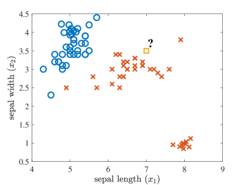
Figure 4.1: Illustration of the binary ($K=2$ classes) classification problem with a domain space of dimension $D=2$: to which class should the new example $x$ be assigned?

Following the taxonomy introduced in Chapter 2, we can distinguish the following modeling approaches, which will be reviewed in the given order throughout the rest of this chapter.

$\bullet$ Discriminative deterministic models: Model directly the deterministic mapping between domain point and label via a parametrized function $t=\hat{t}\left(x\right)$.

$\bullet$ Discriminative probabilistic models: Model the probability of a point $x$ belonging to class $\mathcal{C}_{k}$ via a parametrized conditional pmf $p(t|x),$ with the relationship between $t$ and $\mathcal{C}_{k}$ defined in (4.4). We will also write $p(\mathcal{C}_{k}|x)$ for the discriminative probability when more convenient.

$\bullet$ Generative probabilistic model: Model the joint distribution of domain point and class label by specifying the prior distribution $p(t)$, or $p(\mathcal{C}_{k})$, and the class-dependent probability distribution $p(x|t)$, or $p(x|\mathcal{C}_{k})$, of the domain points within each class.

Discriminative models are arguably to be considered as setting the current state of the art on classification, including popular methods such as Support Vector Machine (SVM) and deep neural networks. Generative models are potentially more flexible and powerful as they allow to capture distinct class-dependent properties of the covariates $x$.

4.3 Discriminative Deterministic Models

In this section, we discuss binary classification using discriminative deterministic models. Owing to their practical importance and to their intuitive geometric properties, we focus on linear models, whereby the binary prediction $\hat{t}(x)$ is obtained by applying a threshold rule on a decision variable $a(x,\tilde{w})$ obtained as a linear function of the learnable weights $\tilde{w}$ (the notation will be introduced below). Note that the decision variable $a(x,\tilde{w})$ may not be a linear function of the covariates $x$. As we will discuss, this class of models underlie important algorithms that are extensively used in practical applications such as SVM. A brief discussion on multi-class classification using deterministic models is provided at the end of this section. In the next two sections, we cover discriminative probabilistic models, including GLMs and more general models.

4.3.1 Model

In their simplest form, linear discriminative deterministic classification models are of the form

$$\hat{t}(x,\tilde{w})=\textrm{sign}\left(a(x,\tilde{w})\right),$$ (4.5)

where the activation, or decision variable, is given as

$$a(x,\tilde{w}) =\sum_{d=1}^{D}w_{d}x_{d}+w_{0}$$

$$=w^{T}x+w_{0}=\tilde{w}^{T}\tilde{x},$$ (4.6)

and we have defined the weight vectors $w=[w_{1}\cdots w_{D}]^{T}$ and $\tilde{w}=[w_{0}\textrm{ }w_{1}\cdots w_{D}]^{T}$, as well as the extended domain point $\tilde{x}=[1\textrm{ }x^{T}]^{T},$ with $x=[x_{1}\cdots x_{D}]^{T}$. The sign function in decision rule (4.5) outputs 1 if its argument is positive, and 0 or $-1$ if the argument is negative depending on the assumed association rule in (4.4).

Geometric interpretation: classification, geometric and functional margins. The decision rule (4.5) defines a hyperplane that separates the domain points classified as belonging to either of the two classes. A hyperplane is a line when $D=2$; a plane when $D=3$; and, more generally, a $D-1$-dimensional affine subspace [Boyd] in the domain space. The hyperplane is defined by the equation $a(x,\tilde{w})=0$, with points on either side characterized by either positive or negative values of the activation $a(x,\tilde{w}).$ The decision hyperplane can be identified as described in Fig. 4.2: the vector $w$ defines the direction perpendicular to the hyperplane and $-w_{0}/\left|\left|w\right|\right|$ is the bias of the decision surface in the direction $w$.//

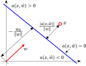
Figure 4.2: Key definitions for a binary linear classifier.

Given a point $x$, it is useful to measure the confidence level at which the classifier assigns $x$ to the class identified through rule (4.5). This can be done by quantifying the Euclidean distance between $x$ and the decision hyperplane. As illustrated in Fig. 4.2, this distance, also known as classification margin, can be computed as $|a\left(x,\tilde{w}\right)|/\left\|w\right\|$.

A point $x$ has a true label $t$, which may or may not coincide with the one assigned by rule (4.5). To account for this, we augment the definition of margin by giving a positive sign to correctly classified points and a negative sign to incorrectly classified points. Assuming that $t$ takes values in $\{-1,1\}$, this yields the definition of geometric margin as

$$\textrm{}\frac{t\cdot a\left(x,\tilde{w}\right)}{\left\|w\right\|},$$ (4.7)

whose absolute value equals the classification margin. For future reference, we also define the functional margin as $\textrm{$t\cdot a\left(x,\tilde{w}\right)$}.$

Feature-based model. The model described above, in which the activation is a linear function of the input variables $x$, has the following drawbacks.

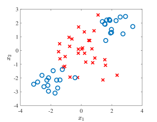
Figure 4.3: A non-linearly separable training set.

1) Bias: As suggested by the example in Fig. 4.3, dividing the domain of the covariates $x$ by means of a hyperplane may fail to capture the geometric structure of the data. In particular, in the example, the two classes are not linearly separable in the space of the covariates – no hyperplane separates exactly the domain points in the two classes. In such cases, classifiers of the form (4.5) may yield large average losses due to the bias induced by the choice of the model (see Sec. 2.3.3).

2) Overfitting: When $D$ is large and the data points $N$ are insufficient, learning the $D+1$ weights of the classifier may cause overfitting.

3) Data-dependent domain size: In some applications, the dimension $D$ may even change from data point to data point, that is, it may vary with the index $n$. For example, a text $x_{n}$, e.g., represented in ASCII format, will have a different dimension $D_{n}$ depending on the number of words in the text.

To address these problems, a powerful approach is that of working with feature vectors $\phi_{k}(x),\quad k=1,\ldots,D^{\prime},$ rather than directly with the covariates $x$, as the input to the classifier. A feature $\phi_{k}(x)$ is a, generally non-linear, function of the vector $x$. It is important to emphasize that these functions are fixed and not learned.

Choosing a number of features $D^{\prime}>D$, which yields an overcomplete representation of the data point $x$, may help against bias; while opting for an undercomplete representation with $D^{\prime}<D$ may help solve the problem of overfitting. Furthermore, the same number of features $D^{\prime}$, e.g., word counts in a bag-of-words model, may be selected irrespective of the size of the data point, addressing also the last problem listed above.

The feature-based model can be expressed as (4.5) with activation

$$a\left(x,\tilde{w}\right)=\sum_{k=1}^{D^{\prime}}w_{k}\phi_{k}(x)=\tilde{w}^{T}\mathbf{\phi}(x),$$ (4.8)

where we have defined the feature vector $\mathbf{\phi}(x)=[\phi_{1}(x)\cdots\phi_{D^{\prime}}(x)]^{T}$. Note that model (4.5) is a special case of (4.8) with the choice $\phi(x)=[1\textrm{ $x^{T}]^{T}$}$.

4.3.2 Learning

As seen in Sec. 2.3.3, learning of deterministic discriminative models can be carried out by means of ERM for a given loss function $\ell$. Furthermore, as discussed in Sec. 2.3.5, overfitting can be controlled by introducing a regularization function $R(\tilde{w})$ on the weight vector $\tilde{w}$. Accordingly, a deterministic predictor $\hat{t}(x,\tilde{w})$ as defined in (4.5) can be learned by solving the regularized ERM problem

$$\underset{\tilde{w}}{\mbox{min}}\quad L_{\mathcal{D}}(\tilde{w})+\frac{\lambda}{N}R(\tilde{w}),$$ (4.9)

with the empirical risk

$$L_{\mathcal{D}}(\tilde{w})=\frac{1}{N}\sum_{n=1}^{N}\ell\left(t_{n},\hat{t}(x_{n},\tilde{w})\right).$$ (4.10)

In (4.9), the hyperparameter $\lambda$ should be selected via validation as explained in Sec. 2.3.5.

Extending the examples discussed in Sec. 2.3.5, the regularization term is typically convex but possibly not differentiable, e.g., $R\left(\tilde{w}\right)=\left\|\tilde{w}\right\|{}_{1}$. Furthermore, a natural choice for the loss function is the 0-1 loss, which implies that the generalization loss $L_{p}$ in (2.2) is the probability of classification error.

In the special case of linearly separable data sets, the resulting ERM problem can be converted to a Linear Program (LP) [Shalev]. Since it is in practice impossible to guarantee the separability condition a priori, one needs generally to solve directly the ERM problem (4.9). The function sign$(\cdot)$ has zero derivative almost everywhere, and is not differentiable when the argument is zero. For this reason, it is difficult to tackle problem (4.9) via standard gradient-based optimization algorithms such as SGD. It is instead often useful to consider surrogate loss functions $\ell(t,a)$ that depend directly on the differentiable (affine) activation $a(x,\tilde{w})$. The surrogate loss function should preferably be convex in $a$, and hence in $\tilde{w}$, ensuring that the resulting regularized ERM problem

$$\underset{\tilde{w}}{\mbox{min}}\quad\sum_{n=1}^{N}\ell(t_{n},a(x_{n},\tilde{w}))+\frac{\lambda}{N}R(\tilde{w})$$ (4.11)

is convex. This facilitates optimization [Boyd], and, under suitable additional conditions, guarantees generalization [Shalev] (see also next chapter). The surrogate loss function should also ideally be an upper bound on the original loss function. In this way, the actual average loss is guaranteed to be smaller than the value attained under the surrogate loss function. Examples of surrogate functions that will be considered in the following can be found in Fig. 4.4.

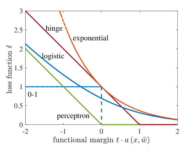
Figure 4.4: Some notable surrogate loss functions for binary classification along with the 0-1 loss.

Perceptron Algorithm

The perceptron algorithm is one of the very first machine learning and AI algorithms. It was introduced by Frank Rosenblatt at the Cornell Aeronautical Laboratory in 1957 to much fanfare in the popular press – it is “the embryo of an electronic computer that [the Navy] expects will be able to walk, talk, see, write, reproduce itself and be conscious of its existence.” reported The New York Times [NYT1]. The algorithm was implemented using analog electronics and demonstrated impressive – for the time – classification performance on images [Bishop].

Using the feature-based model for generality, the perceptron algorithm attempts to solve problem (4.11) with the surrogate perceptron loss function defined as

$$\ell(t,a(x,\tilde{w})) =\max\left(0,-\textrm{$t\cdot a\left(x,\tilde{w}\right)$}\right).$$ (4.12)

The perceptron loss assigns zero cost to a correctly classified example $x$, whose functional margin $t\cdot a\left(x,\tilde{w}\right)$ is positive, and a cost equal to the absolute value of the functional margin for a misclassified example, whose functional margin is negative. A comparison with the 0-1 loss is shown in Fig. 4.4. The perceptron algorithm tackles problem (4.11) with $\lambda=0$ via SGD with mini-batch size $S=1$. The resulting algorithm works as follows. First, the weights $\tilde{w}^{(0)}$ are initialized. Then, for each iteration $i=1,2,...$

$\bullet$ Pick a training example ($x_{n},t_{n}$) uniformly with replacement from $\mathcal{D}$;

$\bullet$ If the example is correctly classified, i.e., if $\textrm{$t_{n}a(x_{n},\tilde{w}$)}\geq 0$, do not update the weights: $\tilde{w}^{(i)}\leftarrow\tilde{w}^{(i-1)}$;

$\bullet$ If the example is not correctly classified, i.e., if $t_{n}a(x_{n},\tilde{w})<0$, update the weights as:

$$\tilde{w}^{(i)} \leftarrow\tilde{w}^{(i-1)}-\nabla_{\tilde{w}}\ell(t_{n},a(x_{n},\tilde{w}))|_{\tilde{w}=\tilde{w}^{(i-1)}}=\tilde{w}^{(i-1)}+\phi(x_{n})t_{n}.$$ (4.13)

It can be proved that, at each step, the algorithm reduces the term $\ell(t_{n},a(x_{n},\tilde{w}))$ in the perceptron loss related to the selected training example $n$ if the latter is misclassified. It can also be shown that, if the training set is linearly separable, the perceptron algorithm finds a weight vector $\tilde{w}$ that separates the two classes exactly in a finite number of steps [Bishop]. However, convergence can be slow. More importantly, the perceptron fails on training sets that are not linearly separable, such as the “XOR” training set $\mathcal{D}$=$\{([0,0]^{T},0),([0,1]^{T},1),([1,0]^{T},1),([1,1]^{T},0)\}$ [minsky1969perceptrons]. This realization came as a disappointment and contributed to the first so-called AI winter period characterized by a reduced funding for AI and machine learning research [WikiAI].

Support Vector Machine (SVM)

SVM, introduced in its modern form by Cortes and Vapnik [cortes1995support] in 1995, was among the main causes for a renewal of interest in machine learning and AI. For this section, we will write explicitly (and with a slight abuse of notation) the activation as

$$a\left(x,\tilde{w}\right)=w_{0}+w^{T}\phi(x),$$ (4.14)

in order to emphasize the offset $w_{0}$. SVM solves the regularized ERM problem (4.11) with the surrogate hinge loss function

$$\ell(t,a(x,\tilde{w})) =\max(0,1-\textrm{$t\cdot a\left(x,\tilde{w}\right)$}),$$ (4.15)

and with the regularization function $R(\tilde{w})=\left\|w\right\|^{2}$. Note that the latter involves only the vector $w$ and not the bias weight $w_{0}$ – we will see below why this is a sensible choice. The hinge loss function is also shown in Fig. 4.4.

Therefore, unlike the perceptron algorithm, SVM includes a regularization term, which was shown to ensure strong theoretical guarantees in terms of generalization error [cristianini2000introduction]. Furthermore, rather than relying on SGD, SVM attempts to directly solve the regularized ERM problem using powerful convex optimization techniques [Boyd].

To start, we need to deal with the non-differentiability of the hinge loss (4.15). This can be done by introducing auxiliary variables $z_{n}$, one for each training example $n$. In fact, imposing the inequality $z_{n}\geq\ell(t_{n},a(x_{n},\tilde{w}))$ yields the following equivalent problem

$$\underset{\tilde{w},z}{\mbox{min}} \sum_{n=1}^{N}z_{n}+\frac{\lambda}{N}\left\|w\right\|^{2}$$ (4.16a)

s.t. $$t_{n}\cdot a(x_{n},\tilde{w})\geq 1-z_{n}$$ (4.16b)

$$z_{n}\geq 0\textrm{ for $n$=$1,...,N$},$$ (4.16c)

where $z=[z_{1}\cdots z_{N}]^{T}$. The equivalence between the original regularized ERM problem and problem (4.16) follows from the fact that any optimal value of the variables ($\tilde{w},z$) must satisfy either constraint (4.16b) or (4.16c) with equality. This can be seen by contradiction: a solution for which both constraints are loose for some $n$ could always be improved by decreasing the value of the corresponding variables $z_{n}$ until the most stringent of the two constraints in (4.16) is met. As a consequence, at an optimal solution, we have the equality $z_{n}=\ell(t_{n},a(x_{n},\tilde{w}))$.

The advantage of formulation (4.16) is that the problem is convex, and can hence be solved using powerful convex optimization techniques [Boyd]. In fact, the cost function is strictly convex, and thus the optimal solution is unique [Boyd]. Furthermore, the optimal solution has an interesting interpretation in the special case in which the training data set is linearly separable. As we will see, this interpretation justifies the name of this technique.

Linearly separable sets and support vectors. When the data set is linearly separable, it is possible to find a vector $\tilde{w}$ such that all points are correctly classified, and hence all the functional margins are positive, i.e., $t_{n}\cdot a(x_{n},\tilde{w})>0$ for $n=1,...,N$. Moreover, by scaling the vector $\tilde{w}$, it is always possible to ensure that the minimum functional margin equals 1 (or any other positive value). This means that we can impose without loss of optimality the inequalities $t_{n}\cdot a(x_{n},\tilde{w})\geq 1$ for $n=1,...,N$ and hence set $z=0$ in problem (4.16). This yields the optimization problem

$$\underset{\tilde{w}}{\mbox{min}} \left\|w\right\|^{2}$$ (4.17a)

s.t. $$\textrm{$\text{$t_{n}\cdot a(x_{n},\tilde{w})\geq 1$}$}\textrm{ for $n$=$1,...,N$}.$$ (4.17b)

The problem above can be interpreted as the maximization of the minimum geometric margin across all training points. To see this, note that, under the constraint (4.17b), the minimum geometric margin can be computed as

$$\underset{n=1,...,N}{\textrm{min}}\frac{t_{n}a(x_{n},\tilde{w})}{\left\|w\right\|}=\frac{1}{\left\|w\right\|}.$$ (4.18)

Furthermore, we call the vectors that satisfy the constraints (4.17b) with equality, i.e., $t_{n}\cdot a(x_{n},\tilde{w})=1$, as support vectors, since they support the hyperplanes parallel to the decision hyperplane at the minimum geometric margin. At an optimum value $\tilde{w}$, there are at least two support vectors, one on either side of the separating hyperplane (see [Bishop, Fig. 7.1]).

Using Lagrange duality, the support vectors can be easily identified by observing the optimal values $\{\alpha_{n}\}$ of the multipliers associated with the constraints (4.16b). Support vectors $x_{n}$ correspond to positive Lagrange multipliers $\alpha_{n}>0$ (see, e.g., [Bishop]), while all other points have zero Lagrange multipliers. Note that the Lagrange multipliers are returned by standard solvers such as the ones implemented by the CVX toolbox in MATLAB [cvx].

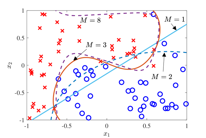
Figure 4.5: Example of binary classification with SVM using polynomial features up to degree $M$ ($\lambda/N=0.2$).

Example 4.3.1.

In the example in Fig. 4.5, the illustrated $N=80$ training samples are fed to a SVM using the monomial feature vector $\phi(x)=[1\textrm{ $x_{1}\textrm{ }$$x_{2}\cdots x_{1}^{M}\textrm{ $x_{2}^{M}$}]$}$ and $\lambda/N=0.2$ for given model orders $M$. The decision boundary is shown using dashed and solid lines. It is seen that, using a sufficiently large order (here $M=3$), SVM is able to effectively partition the two samples in the two classes. Furthermore, even with larger values of $M$ (here $M=8$), SVM appears not to suffer from significant overfitting thanks to the quadratic regularization term.

The optimization problem (4.16) may be conveniently tackled by using Lagrange duality techniques. This approach also allows one to naturally introduce the powerful tool of kernel methods. The interested reader can find this discussion in Appendix B of this chapter.

4.3.3 Multi-Class Classification^∗

Here we briefly describe classification scenarios with $K>2$ classes. As a first observation, it is possible to build multi-class classifiers based solely on multiple binary classifiers, such as SVM. This can be done by following one of two general strategies, namely one-versus-the-rest and one-versus-one [Bishop, Chapter 7]. The one-versus-the-rest approach trains $K$ separate binary classifiers, say $k=1,...,K$, with the $k$th classifier operating on the examples relative to class $\mathcal{C}_{k}$ against the examples from all other classes. The one-versus-one method, instead, trains $K(K-1)/2$ binary classifiers, one for each pair of classes. Both approaches can yield ambiguities in classification [Bishop, Chapter 7].

4.4 Discriminative Probabilistic Models: Generalized Linear Models

Discriminative probabilistic models are potentially more powerful than deterministic ones since they allow to model sources of uncertainty in the label assignment to the input variables. This randomness may model noise, labelling errors, e.g., for crowdsourced labels, and/or the residual uncertainty in the classification rule due to the availability of limited data. Probabilistic models can also more naturally accommodate the presence of more than two classes by producing a probability distribution over the possible label values.

In this section, we study GLMs, which were introduced in Sec. 3.5. We recall that a GLM (3.54) posits that the conditional pmf $p(t|x),$ or $p(\mathcal{C}_{k}|x)$, is a member of the exponential family in which the natural parameter vector $\eta$ is given as a linear function of a feature vector $\phi(x)$, i.e., $\eta=W\phi(x)$ for weight matrix $W$. It is noted that GLMs are not linear: only the unnormalized log-likelihood is linear in the weight matrix $W$ (see Sec. 3.2). We start by discussing binary classification and then cover the multi-class case in Sec. 4.4.3.

4.4.1 Model

For classification, the label $t$ can take a finite number of values, and it can hence be described by a Bernoulli variable in the binary case or, more generally, by a Categorial variable (see Chapter 3). The GLM (3.54) for binary classification is known as logistic regression, and it assumes the predictive distribution

$$p(t=1|x)=\sigma(\tilde{w}^{T}\phi(x)).$$ (4.19)

We recall that $\sigma(a)=(1+\exp(-a))^{-1}$ is the sigmoid function (see Chapter 2). We also observe that

$$\sigma(-a)=1-\sigma(a),$$ (4.20)

which implies that we can write $p(t=0|x)=1-\sigma(\tilde{w}^{T}\phi(x))=\sigma(-\tilde{w}^{T}\phi(x))$. Intuitively, the sigmoid function in (4.19) can be thought of as a “soft” version of the threshold function $\textrm{sign}(a)$ used by the deterministic models studied in the previous section.

We emphasize that the logistic regression model (4.19) is a GLM since it amounts to a Bernoulli distribution, which is in the exponential family, with natural parameter vector $\eta=\tilde{w}^{T}\phi(x)$ as in

$$t|x,w\sim\text{Bern}(t|\eta=\tilde{w}^{T}\phi(x)).$$ (4.21)

Inference. Before discussing learning, we observe that inference is straightforward. In fact, once the discriminative model (4.19) is known, the average 0-1 loss, that is, the probability of error, is minimized by choosing the label according to the following rule

$$p(\mathcal{C}_{1}|x)=p(t=1|x)\underset{\mathcal{C}_{0}}{\overset{\mathcal{C}_{1}}{\gtrless}}\frac{1}{2},$$ (4.22)

or equivalently $\tilde{w}^{T}\phi(x)\underset{\mathcal{C}_{0}}{\overset{\mathcal{C}_{1}}{\gtrless}}0$.

4.4.2 Learning

Consider first ML. The NLL function can be written as

$$-\ln p(t_{\mathcal{D}}|x_{\mathcal{D}},\tilde{w}) =-\sum_{n=1}^{N}\ln p(t_{n}|x_{n},\tilde{w})$$ (4.23)

$$=-\sum_{n=1}^{N}\{t_{n}\ln(y_{n})+(1-t_{n})\ln(1-y_{n})\},$$ (4.24)

where we have defined $y_{n}=\sigma(\tilde{w}^{T}\phi(x_{n}))$. The NLL (4.23) is also referred to as the cross entropy loss criterion, since the term $-t\ln(y)-(1-t)\ln(1-y)$ is the cross-entropy $H((t,1-t)||(y,1-y))$ (see Sec. 2.6). We note that the cross-entropy can be used to obtain upper bounds on the probability of error (see, e.g., [2018arXiv180209386F]). The ML problem of minimizing the NLL is convex (see Sec. 3.1), and hence it can be solved either directly using convex optimization tools, or by using iterative methods such as SGD or Newton (the latter yields the iterative reweighed least square algorithm [Bishop, p. 207]).

The development of these methods leverages the expression of the gradient of the LL function (3.28) (used with $N=1$) for the exponential family. To elaborate, using the chain rule for differentiation, we can write the gradient

$$\nabla_{\tilde{w}}\ln p(t|x,\tilde{w})=\nabla_{\eta}\ln\textrm{Bern}(t|\eta)|_{\eta=\tilde{w}\phi(x)}\times\nabla_{\tilde{w}}(\tilde{w}^{T}\phi(x)),$$ (4.25)

which, recalling that $\text{$\nabla_{\eta}$ln$($Bern}(t|\eta))=(t-\sigma(\eta))$ (cf. (3.28)), yields

$$\nabla_{\tilde{w}}\ln p(t|x,\tilde{w})=(t-y)\phi(x).$$ (4.26)

Evaluating the exact posterior distribution for the Bayesian approach turns out to be generally intractable due to the difficulty in normalizing the posterior

$$p(w|\mathcal{\mathcal{D}})\propto p(w)\prod_{n=1}^{N}p(t_{n}|x_{n},\tilde{w}).$$ (4.27)

We refer to [Bishop, p. 217-220] for an approximate solution based on Laplace approximation. Other useful approximate methods will be discussed in Chapter 8.

As a final remark, with bipolar labels, i.e., $t$$\in\{-1,+1\}$, the cross-entropy loss function can be written as

$$-\ln p(t_{\mathcal{D}}|x_{\mathcal{D}},\tilde{w})=\sum_{n=1}^{N}\ln(1+\exp(-t_{n}a(x_{n},\tilde{w})).$$ (4.28)

This formulation shows that logistic regression can be thought of as an ERM method with loss function $\ell(t,a(x,\tilde{w}))=\ln(1+\exp(-ta(\mathrm{x},\tilde{w})),$ which is seen in Fig. 4.4 to be a convex surrogate loss of the 0-1 loss.

Mixture models.^∗ As seen, the Bayesian approach obtains the predictive distribution by averaging over multiple models $p(t|x,w)$ with respect to the parameters’ posterior $p(w|\mathcal{D})$ (cf. (2.34)). The resulting model hence mixes the predictions returned by multiple discriminative models $p(t|x,w)$ to obtain the predictive distribution $p(t|x)=\int p(w|\mathcal{D})p(t|x,w)dw$. As we briefly discuss below, it is also possible to learn mixture models within a frequentist framework.

Consider $K$ probabilistic discriminative models $p(t|x,w_{k})$, $k=1,...,K$, such as logistic regression. The mixture model is defined as

$$p(t|x,\theta)=\sum_{k=1}^{K}\pi_{k}p(t|x,w_{k}).$$ (4.29)

In this model, the vector $\theta$ of learnable parameters includes the probability vector $\pi$, which defines the relative weight of the $K$ models, and the vectors $w_{1},...,w_{K}$ for the $K$ constituent models. As discussed, in the Bayesian approach, the weights $\pi_{k}$ are directly obtained by using the rules of probability, as done in (4.27). Within a frequentist approach, instead, ML training is typically performed via a specialized algorithm, which will be described in Chapter 6, known as Expectation Maximization (EM).

Mixture models increase the capacity of discriminative models and hence allow to learn more complex relationships between covariates and labels. In particular, a mixture model, such as (4.29), has a number of parameters that increases proportionally with the number $K$ of constituent models. Therefore, the capacity of a mixture model grows larger with $K$. As an example, this increased capacity may be leveraged by specializing each constituent model $p(t|x,w_{k})$ to a different area of the covariate domain.

Given their larger capacity, mixture models may be prone to overfitting. A way to control overfitting will be discussed in Sec. 4.7.

4.4.3 Multi-Class Classification

In the case of $K$ classes, the relevant exponential family distribution is Categorical with natural parameters depending linearly on the feature vector. This yields the following discriminative model as a generalization of logistic regression

$$\mathrm{t}|x,W\sim\text{Cat}(t|\eta=W\phi(x)),$$ (4.30)

where the label vector $\mathrm{t}$ is defined using one-hot encoding (Chapter 3) and $W$ is a matrix of weights. We can also equivalently write the vector of probabilities for the $K$ classes as

$$y=\textrm{softmax($W\phi(x)$)=}\begin{bmatrix}\frac{e^{\eta_{0}}}{\sum_{k=0}^{K-1}e^{\eta_{k}}}\\ \vdots\\ \frac{e^{\eta_{K-1}}}{\sum_{k=0}^{K-1}e^{\eta_{k}}}\end{bmatrix},$$ (4.31)

where $y=[y_{1}\cdots y_{K}]^{T}$ with $y_{k}=p(\mathcal{C}_{k}|x)$; and $\eta_{k}=w_{k+1}^{T}\phi(x)$ with $w_{k}^{T}$ being the $k$th row of the weight matrix $W$.

Learning follows as for logistic regression. To briefly elaborate on this point, the NLL can be written as the cross-entropy function

$$-\ln p(t_{\mathcal{D}}|x_{\,\mathcal{D}},W) =-\sum_{n=1}^{N}\ln p(t_{n}|x_{n},W)$$

$$=-\sum_{n=1}^{N}t_{n}^{T}\ln(y_{n}),$$ (4.32)

where the logarithm is applied element by element, and we have $y_{n}=\textrm{softmax}(W\phi(x_{n}))$. Note that each term in (4.32) can be expressed as the cross-entropy $-t_{n}^{T}\ln(y_{n})=H(t_{n}||y_{n}).$ The ML problem is again convex and hence efficiently solvable. The gradient of the NLL can be again found using the general formula (3.28) for exponential models and the chain rule for derivatives. We can write

$$\nabla_{W}\ln p(t\text{$|x,W$)=$\nabla$${}_{\eta}$}\ln\textrm{Cat}(t|\eta)|_{\eta=W\phi(x)}\times\nabla_{W}(W\phi(x)),$$ (4.33)

which yields

$$\nabla_{W}\ln p(t|x,W)=(t-y)\phi(x)^{T}.$$ (4.34)

4.4.4 Relation to Neural Networks

GLM models of the form (4.30), or (4.19) in the special case of binary classification, can be interpreted in terms of the neural network shown in Fig. 4.6. A neural network consists of a directed graph of computing elements, known as neurons. Each neuron applies a deterministic transformation of its inputs, as defined by the incoming edges, to produce a scalar output on its outgoing edge.

In Fig. 4.6, the input vector $x$ is first processed by a hidden layer of neurons, in which each $k$th neuron computes the feature $\phi_{k}(x)$. Then, each $k$th neuron in the output layer applies the $k$th element of the softmax non-linearity (4.31) to the numbers produced by the hidden neurons in order to compute the probability $y_{k}=p(\mathcal{C}_{k}|x)$. Note that, in the case of binary classification, only one output neuron is sufficient in order to compute the probability (4.19). It is also important to emphasize that only the weights between hidden and output layers are learned, while the operation of the neurons in the hidden layer is fixed.

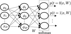
Figure 4.6: GLM as a three-layer neural network with learnable weights only between hidden and output layers.

We remark that one should not confuse a graph such as the one in Fig. 4.6 with the BN representation previously seen in Fig. 2.7, which will be further discussed in Chapter 7. In fact, while BNs represent probability distributions, diagrams of neural networks such as in Fig. 4.6 describe deterministic functional relations among variables. This is despite the fact that the output layer of the network in Fig. 4.6 computes a vector of probabilities. In other words, while the nodes of a BN are rvs, those in the graph of a neural network are computational nodes.

“Extreme machine learning”.^∗ An architecture in which the features $\mathbf{\phi}(x)$ are selected via random linear combinations of the input vector $x$ is sometimes studied under the rubric of “extreme machine learning” [HUANG2006489]. The advantage of this architecture as compared to deep neural networks with more hidden layers and full learning of the weights (Sec. 4.5) is its low complexity.

4.5 Discriminative Probabilistic Models: Beyond GLM

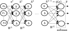
Figure 4.7: A multi-layer neural network.

As depicted in Fig. 4.6, GLMs can be interpreted as three-layer neural networks in which the only hidden layer computes fixed features. The fixed features are then processed by the output classification layer. In various applications, determining suitable features is a complex and time-consuming task that requires significant domain knowledge. Moving beyond GLMs allows us to work with models that learn not only the weights used by the output layer for classification, but also the vector of features $\phi(x)$ on which the output layer operates. This approach yields a much richer set of models, which, along with suitable learning algorithms, has led to widely publicized breakthroughs in applications ranging from speech translation to medical diagnosis.

As a prominent example of beyond-GLM classification models, we describe here feed-forward multi-layer neural networks, or deep neural networks when the hidden layers are in large number. We note that, beside yielding state-of-the-art classification algorithms, multi-layer feedforward networks are also key components of the computational theory of mind [Pinker].

4.5.1 Model

As illustrated in Fig. 4.7, feed-forward multi-layer networks consist of multiple layers with learnable weights. Focusing on multi-class classification, we have the chain of vectors $x\rightarrow h^{1}\rightarrow\cdots\rightarrow h^{L}\rightarrow y$, where $x$ is the $D\times 1$ input (observed) vector; $y$ is the $K\times$1 vector of output probabilities for the $K$ classes; and $h^{l}$ represents the vector of outputs at the $l$th hidden layer. The number of neurons in each hidden layer is a hyperparameter to be optimized via validation or Bayesian methods (Chapter 2). Note that the adopted numbering of the layers is not universally accepted, and the reverse ordering is also used.

Referring to Fig. 4.7, we can write the operation of the neural network through the functional relations

$$h^{1} =h(a^{1})\textrm{ with $a^{1}=W^{1}$}x$$ (4.35a)

$$h^{l} =h(a^{l})\textrm{ }\textrm{with $a^{l}=W^{l}$$h$${}^{l-1}$}$$ (4.35b)

for $$l=2,...,L$$ (4.35c)

$$y =\textrm{softmax}(a^{L+1})\textrm{ with $a^{L+1}$=$W^{L+1}h^{L}$}.$$ (4.35d)

The non-linear function $h(\cdot)$ is applied element-wise and is typically selected as a sigmoid, such as the logistic sigmoid or the hyperbolic tangent, or else, as has become increasingly common, the Rectified Linear Unit (ReLU) $h(a)=\max(0,a).$ In (4.35), we have defined the activation vectors $a^{l}$ for the hidden layers $l=1,...,L$, and the matrices of weights $W^{l}$, $l=1,...,L+1$, whose dimensions depend on the size of the hidden layers. We denote the tensor of all weights as $W$.

The learnable weights of the hidden layers encode the feature vector $\phi(x)=h_{L}$ used by the last layer for classification. With multi-layer networks, we have then moved from having fixed features defined a priori by vector $\phi(x)$ in linear models to designing optimal features that maximize the classifier’s performance in non-linear models. Furthermore, in multi-layer networks, the learned features $h^{1},...,h^{L}$ tend to progress from low-level features in the lower layers, such as edges in an image, to higher-level concepts and categories, such as “cats” or “dogs”, in the higher layers [Goodfellowbook].

4.5.2 Learning

Training deep neural networks is an art [Goodfellowbook]. The basic underlying algorithm is backpropagation, first proposed in 1969 and then reinvented in the mid-1980s [norvig2009, Rumelhart]. However, in practice, a number of tricks are required in order to obtain state-of-the-art performance, including methods to combat overfitting, such as dropout. Covering these solutions would require a separate treatise, and here we refer to [Hintoncourse, Goodfellowbook] for an extensive discussion.

Backpropagation – or backprop for short – extends the derivation done in (4.34) to evaluate the gradient of the LL to be used within an SGD-based algorithm. Again, the main ingredients are the general formula (3.28) for exponential models and the chain rule for derivatives. To elaborate, select a given training example $(x_{n},t_{n})=(x,t)$ to be used in an iteration of SGD. Backprop computes the derivative of the NLL, or cross-entropy loss function, $L(W)=-\ln p(t|x,W)=-t^{T}\ln y$ (cf. (4.32)), where the output $y$ is obtained via the relations (4.35). It is important to note that, unlike the linear models studied above, the cross-entropy for multi-layer is generally a non-convex function of the weights.

Backprop computes the gradients with respect to the weight matrices by carrying out the following phases.

$\bullet$ Forward pass: Given $x$, apply formulas (4.35) to evaluate $a^{1},h^{1},a{}^{2},$ $h^{2},...,a^{L},h^{L},\textrm{ and }y.$

$\bullet$ Backward pass: Given $a^{1},h^{1},a{}^{2},$$h^{2},...,a^{L},h^{L},a^{L+1},y$ and $t$, compute

$$\delta^{L+1} =(y-t)$$ (4.36a)

$$\delta^{l} =(W^{l+1})^{T}\delta^{l+1}\cdot h^{\prime}(a^{l})\textrm{ { for $l=L,L-1,...,1$}}$$ (4.36b)

$$\nabla_{W^{l}}L(W) =\delta^{l}(h^{l-1})^{T}\textrm{ for $l=1,2,...,L+1$},$$ (4.36c)

where $h^{\prime}(\cdot)$ denotes the first derivative of the function $h(\cdot)$; the product $\cdot$ is taken element-wise; and we set $h^{0}=x$.

Backprop requires a forward pass and a backward pass for every considered training example. The forward pass uses the neural network as defined by equations (4.35). This entails multiplications by the weight matrices $W^{l}$ in order to compute the activation vectors, as well as applications of the non-linear function $h(\cdot)$. In contrast, the backward pass requires only linear operations, which, by (4.36b), are based on the transpose $(W^{l})^{T}$ of the weight matrix $W^{l}$ used in the forward pass.

The derivatives (4.36c) computed during the backward pass are of the general form

$$\nabla_{w_{ij}^{l}}L(W)=h_{i}^{l-1}\times\delta_{j}^{l},$$ (4.37)

where $w_{ij}^{l}$ is the $(i,j)$th element of matrix $W^{l}$ corresponding to the weight between the pre-synaptic neuron $j$ in layer $l-1$ and the post-synaptic neuron $i$ in layer $l$; $h_{i}^{l-1}$ is the output of the pre-synaptic neuron $i$; and $\delta_{j}^{l}$ is the back-propagated error. The back-propagated error assigns “responsibility” for the error $y-t$ measured at the last layer (layer $L+1$) to each synaptic weight $w_{ij}^{l}$ between neuron $j$ in layer $l-1$ and neuron $i$ in layer $l$. The back-propagated error is obtained via the linear operations in (4.36b).

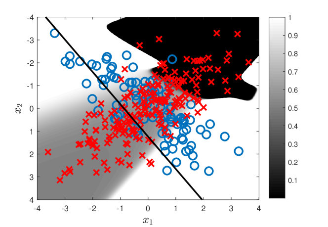
Figure 4.8: Probability that the class label is the same as for the examples marked with circles according to the output of a feed-forward multi-layer network with one hidden layer ($L=1$) and six hidden neurons (with sigmoid non-linearity). The probability is represented by the color map illustrated by the bar on the right of the figure. For reference, the solid line represent the decision line for logistic regression.

Example 4.5.1.

In the example in Fig. 4.8, the illustrated $N=300$ training examples are used to train a logistic regression, i.e., GLM, model and a feed-forward multi-layer network with one hidden layer ($L=1$) and six hidden neurons with sigmoid non-linearity $h(x)=\sigma(x)$. The logistic model uses linear features $\phi(x)=[1\textrm{ $x$}]^{T}$. Both networks are trained using SGD. For logistic regression, the decision line is illustrated as a solid line, while for the multi-layer network we plot the probability that the class label is the same as for the examples marked with circles as color map. The GLM model with linear features is seen to be unable to capture the structure of the data, while the multi-layer network can learn suitable features that improve the effectiveness of classification.

4.5.3 Some Advanced Topics^∗

We conclude this section by noting a few important aspects of the ongoing research on deep neural networks.

A first issue concerns the theoretical understanding of the generalization properties of deep neural networks. On the face of it, the success of deep neural networks appears to defy one of the the principles laid out in Chapter 2, which will be formalized in the next chapter: Highly over-parametrized models trained via ML suffer from overfitting and hence do not generalize well. Recent results suggest that the use of SGD, based on the gradient (4.37), may act a regularizer following an MDL perspective. In fact, SGD favors the attainment of flat local maxima of the likelihood function. Flat maxima require a smaller number of bits to be specified with respect to sharp maxima, since, in flat maxima, the parameter vector can be described with limited precision as long as it remain within the flat region of the likelihood function [hochreiter1997flat, keskar2016large, Ferenc] (see also [kawaguchi] for a different perspective).

Another important aspect concerns the hardware implementation of backprop. This is becoming extremely relevant given the practical applications of deep neural networks for consumer’s devices. In fact, a key aspect of backprop is the need to propagate the error, which is measured at the last layer, to each synapse via the backward pass. This is needed in order to evaluate the gradient (4.37). While a software implementation of this rule does not present any conceptual difficulty, realizing the computations in (4.36) in hardware, or even on a biological neural system, is faced with a number of issues.

A first problem is the non-locality of the update (4.37). An update rule is local if it only uses information available at each neuron. In contrast, as seen, rule (4.37) requires back-propagation through the neural network. Another issue is the need for the backward pass to use a different neural path with respect to the forward pass, given that, unlike the backward pass, the forward pass includes also non-linearities. A useful discussion of hardware implementation aspects can be found in [baldi2016learning] (see also references therein).

To obviate at least some of these practical issues, a number of variations of the rule (4.37) have been proposed [baldi2016learning]. For instance, the feedback alignment rule modifies (4.36b) by using fixed random matrices in lieu of the current weight matrices $W^{l}$; while the broadcast alignment rule writes the vectors $\delta^{l}$ as a linear function with fixed random coefficients of the error ($y-t$), hence removing the need for back-propagation [Samadi17].

Furthermore, beside ML, there exist Bayesian learning algorithms [Gal2016Uncertainty], including simplified approaches such as dropout [Goodfellowbook, Hintoncourse]. Significant progress has also been made on applications such as image recognition by leveraging the underlying structure, or geometry, of the data [bronstein2017geometric]. As an important case in point, convolutional neural networks leverage the stationarity, locality and spatial invariance of image features by limiting the receptive field of the neurons (i.e., by setting to zero weights that connect to “distant” pixels) and by tying the weights of neurons in the same layer.

Another recent development is the design of event-driven spiking neural networks that can be implemented on neuromorphic computing platforms with extremely low energy consumption (see, e.g., [neuromorphic, 2017arXiv171010704B]).

4.6 Generative Probabilistic Models

As discussed in Chapter 2, discriminative models do not attempt to model the distribution of the domain points $x$, learning only the predictive distribution $p(t|x)$. In contrast, generative models aim at modelling the joint distribution by specifying parametrized versions of the prior distribution $p(t)$, or $p(\mathcal{C}_{k})$, and of the class-conditional probability distribution $p(x|t)$, or $p(x|\mathcal{C}_{k})$. As a result, generative models make more assumptions about the data by considering also the distribution of the covariates $\mathrm{x}$. As such, generative models may suffer from bias when the model is incorrectly selected. However, the capability to capture the properties of the distribution of the explanatory variables $\mathrm{x}$ can improve learning if the class-conditional distribution $p(x|t)$ has significant structure.

4.6.1 Model

Generative models for binary classification are typically defined as follows

$$\mathrm{t} \sim\text{Bern}(\pi)$$ (4.38a)

$$\mathrm{x}|\mathrm{t}=t \sim\text{exponential}(\eta_{t}),$$ (4.38b)

where $\text{exponential}(\eta)$ represents a distribution from the exponential family with natural parameter vector $\eta$ (see previous chapter). Accordingly, the parameters of the model are $\theta=(\pi,\text{$\eta$}_{0},\eta_{1})$, where vectors $\text{$\eta$}_{t}$ represent the natural parameters of the class-dependent distributions. As we have seen in Chapter 2, we can also equivalently use mean parameters to define the exponential family distributions. As a result of this choice, the joint distribution for rv $(\mathrm{\mathrm{x}},\mathrm{t})$ is given as $p(x,t|\pi,\text{$\eta$}_{0},\eta_{1})=p(t|\pi)p(x|\text{$\eta$}_{t})$.

Inference. Given a new point $x$, in order to minimize the probability of error, the optimal prediction of the class under 0-1 loss can be seen to satisfy the maximum a posteriori rule

$$p(\mathcal{C}_{1}|x)=\frac{\pi p(x|\eta_{1})}{\pi p(x|\eta_{1})+(1-\pi)p(x|\eta_{0})}\underset{\mathcal{C}_{0}}{\overset{\mathcal{C}_{1}}{\gtrless}}\frac{1}{2}.$$ (4.39)

4.6.2 Learning

We now focus on ML learning. The LL function can be written as

$$\ln p(\mathcal{D}|\pi,\text{$\eta$}_{0},\eta_{1})=\sum_{n=1}^{N}\ln p(t_{n}|\pi)+\sum_{{n=1:\atop t_{n}=0}}^{N}\ln p(x_{n}|\eta_{0})+\sum_{{n=1:\atop t_{n}=1}}^{N}\ln p(x_{n}|\eta_{1}).$$ (4.40)

Given the decomposition of the LL in (4.40), we can optimize over $\pi$, $\eta_{0}$ and $\eta_{1}$ separately, obtaining the respective ML estimates. Note, however, that, while for $\pi$ we can use the entire data set, the optimization over parameters $\eta_{0}$ and $\eta_{1}$ can leverage smaller data sets that include only the samples $x_{n}$ with labels $t_{n}=0$ or $t_{n}=1$, respectively. As we discussed in Chapter 2, ML estimates of exponential families merely require moment matching, making these estimates generally easy to obtain. We illustrate this point below with two important examples.

Quadratic Discriminant Analysis (QDA). In QDA, the class-dependent distributions are Gaussian with class-dependent mean and covariance:

$$\mathrm{t} \sim\textrm{Bern}(\pi)$$ (4.41a)

$$\mathrm{x}|\mathrm{t} =k\sim\mathcal{N}(\mu_{k},\Sigma_{k}).$$ (4.41b)

By the general rules derived in Chapter 2 for the exponential family, ML selects the moment matching estimates

$$\pi_{ML} =\frac{N[1]}{N}$$ (4.42a)

$$\mu_{k,ML} =\frac{1}{N[k]}\sum_{{n=1:\atop t_{n}=k}}^{N}x_{n}$$ (4.42b)

$$\Sigma_{k,ML} =\frac{1}{N[k]}\sum_{{n=1:\atop t_{n}=k}}^{N}(x_{n}-\mu_{k})(x_{n}-\mu_{k})^{T}.$$ (4.42c)

The resulting predictive distribution for the label of a new sample is then given by (4.39) by plugging in the estimates above as

$$p(\mathcal{C}_{1}|x)=\frac{\pi_{ML}\mathcal{N}(x|\mu_{1,ML},\Sigma_{1,ML})}{\pi_{ML}\mathcal{N}(x|\mu_{1,ML},\Sigma{}_{1,ML})+(1-\pi_{ML})\mathcal{N}(x|\mu_{0,ML},\Sigma_{0,ML})}.$$ (4.43)

Linear Discriminant Analysis (LDA). Setting $\Sigma_{k}=\Sigma$ for both classes $k=1,2$ yields the Linear Discriminant Analysis (LDA) model [Murphy]. Imposing that two generally distinct parameters, such as $\Sigma_{1}$ and $\Sigma_{2}$ are equal is an example of parameter tying or sharing. By reducing the number of parameters to be learned, parameter sharing can reduce overfitting at the potential cost of introducing bias (see Chapter 2).

Under the assumption of conjugate priors, and of a priori independence of the parameters, MAP and Bayesian approaches can be directly obtained by following the derivations discussed in Chapter 2. We refer to [Bishop, Barber, Murphy] for details.

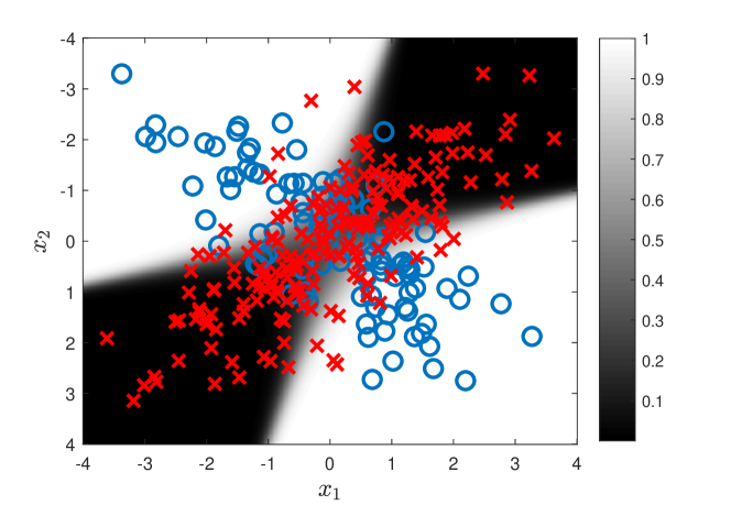
Figure 4.9: Probability that the class label is the same as for the examples marked with circles according to the output of the generative model QDA. The probability is represented by the color map illustrated by the bar on the right of the figure. For this example, it can be seen that LDA fails to separate the two classes (not shown).

Example 4.6.1.

We continue the example in Sec. 4.5 by showing in Fig. 4.9 the probability (4.43) that the class label is the same as for the examples marked with circles according to the output of QDA. Given that the covariates have a structure that is well modelled by a mixture of Gaussians with different covariance matrices, QDA is seen to perform well, arguably better than the discriminative models studied in Sec. 4.5. It is important to note, however, that LDA would fail in this example. This is because a model with equal class-dependent covariance matrices, as assumed by LDA, would entail a significant bias for this example.

4.6.3 Multi-Class Classification^∗

As an example of a generative probabilistic model with multiple classes, we briefly consider the generalization of QDA to $K\geq 2$ classes. Extending (4.41) to multiple classes, the model is described as

$$\mathrm{t} \sim\textrm{Cat}(\pi)$$ (4.44a)

$$\mathrm{x}|\mathrm{t} =k\sim\mathcal{N}(\mu_{k},\Sigma_{k}),$$ (4.44b)

where $\mathrm{t}$ is encoded using one-hot encoding, so that the label of each example is given by the vector $t_{n}=[t_{0n},...,t_{(K-1)n}]^{T}$. Following the discussion above, moment matching yields the ML estimates

$$\pi_{k,ML} =\frac{N[k]}{N}=\frac{\sum_{n=1}^{N}t_{kn}}{N}$$ (4.45a)

$$\mu_{k,ML} =\frac{1}{N[k]}\sum_{n=1}^{N}t_{kn}x_{n}$$ (4.45b)

$$\Sigma_{k,ML} =\frac{1}{N[k]}\sum_{n=1}^{N}t_{kn}(x_{n}-\mu_{k})(x_{n}-\mu_{k})^{T}.$$ (4.45c)

4.7 Boosting^∗

In this last section, we return to the mixture models of the form (4.29) and discuss a popular training approach to reduce overfitting. We focus on deterministic discriminative models with activations $a_{k}(x,\tilde{w}_{k})$, $k=1,...,K,$ in which the mixture predictor is given as

$$a(x,\tilde{w})=\sum_{k=1}^{K}\pi_{k}a_{k}(x,\tilde{w}_{k})$$ (4.46)

with learnable parameters $\{\pi_{k}\}$ and $\{\tilde{w}_{k}\}$. The technique, known as boosting, trains one model $a_{k}(x,\tilde{w}_{k})$ at a time in a sequential fashion, from $k=1$ to $k=K$, hence adding one predictor at each training step $k$. As a result, boosting increases the capacity of the model in a sequential manner, extending the sum in (4.46) over a growing number of predictors. In this way, one starts by training a model with a large bias, or approximation error; and progressively decreases the bias at the cost of a potentially larger estimation error (see Chapter 2 and the next chapter for further discussion on bias and estimation error). As we will discuss below, each model is trained by solving an ERM problem in which the contribution of a training example is weighted by the error rate of the previously trained models.

To elaborate, boosting – more specifically the AdaBoost scheme – can be described as solving an ERM problem with the exponential loss function $\ell(t,a(x,\tilde{w}))=\exp(-t\cdot a(x,\tilde{w}))$, which is plotted in Fig. 4.4. When training the $k$th model, the outputs $a_{1}(x,\tilde{w}_{1}),...,a_{k-1}(x,\tilde{w}_{k-1})$ of the previously trained models, as well as their weights $\pi_{1},...,\pi_{k-1}$, are kept fixed. Excluding the models $k+1,...,K$, the training loss can be written as

$$\sum_{n=1}^{N}\alpha_{n}^{(k)}\exp(-\pi_{k}t_{n}\cdot a_{k}(x_{n},\tilde{w}_{k})),$$ (4.47)

with the weights

$$\alpha_{n}^{(k)}=\exp\left(-t_{n}\cdot\sum_{j=1}^{k-1}\pi_{j}a_{j}(x_{n},\tilde{w}_{j})\right).$$ (4.48)

An important point is that the weights (4.48) are larger for training samples $n$ with smaller functional margin under the mixture model $\sum_{j=1}^{k-1}\pi_{j}a_{j}(x_{n},\tilde{w}_{j})$. Therefore, when training the $k$th model, we give more importance to examples that fare worse in terms of classification margins under the current mixture model. Note that, at each training step $k$, one trains a simple model, which has the added advantage of reducing the computational complexity as compared to the direct learning of the full training model. We refer to [Bishop, Ch. 14][Shalev, Ch. 10] for further details.

4.8 Summary

This chapter has provided a brief review of the key supervised learning problem of classification. Following the taxonomy put forth in Chapter 2, we have divided learning algorithms according to the type of models used to relate explanatory variables and labels. Specifically, we have described deterministic discriminative models, both linear and non-linear, covering the perceptron algorithm, SVM, and backprop for multi-layer neural networks; probabilistic discriminative models, concentrating on GLM; and probabilistic generative models, including QDA and LDA. We have also introduced the more advanced topics of mixture models and boosting. We finally mention that supervised learning, in the form of classification and regression, can also be used as a building block for the task of sequential decision processing via imitation learning (see, e.g., [Levinerl]).

While this chapter has focused on algorithmic aspects, the next chapter discusses a well-established theoretical framework in which to study the performance of learning for classification.

Appendix A: More on SGD^∗

In this appendix, we provide some discussion on the convergence of SGD and on more advanced optimization techniques.

Convergence

To briefly discuss the convergence properties of SGD, consider first for reference the conventional gradient descent algorithms, which corresponds to choosing the entire training set, i.e., $\mathcal{S}=\{1,...,N\}$, at each iteration. If the function to be optimized is strictly convex, as for the quadratic loss, the algorithm is guaranteed to converge to the (unique) minimum even with a fixed learning rate $\gamma^{(i)}=\gamma,$ as long as the latter is no larger than the inverse of the maximum curvature of the loss function $L$, i.e., $\gamma\leq 1/L$. For twice-differentiable loss functions, the maximum curvature $L$ can be evaluated as the maximum eigenvalue of the Hessian matrix. Functions with finite curvature $L$ are known as Lipschitz smooth. For these functions, the convergence is geometric, and hence the number of iterations needed to obtain an error on the optimal solution equal to $\epsilon$ scales as $\textrm{ln}(1/\epsilon$) (see, e.g., [Aggelos, Chapter 8][cevher2014convex, MAL-058]).

We turn now to the proper SGD algorithm operating with a smaller mini-batch size $S$. If the learning rate schedule is selected so as to satisfy the Robbins–Monro conditions

$$\sum_{i=1}^{\infty}\gamma^{(i)}=\infty\textrm{ and }\sum_{i=1}^{\infty}(\gamma^{(i)})^{2}<\infty,$$ (4.49)

the SGD algorithm is known to converge to the optimal solution of problem (4.9) in the case of strictly convex functions and to stationary points for non-convex functions with bounded curvature (see [Aggelos, Chapter 8] for details). Learning rate schedules that satisfy (4.49) include $\gamma^{(i)}=1/i$. The intuitive reason for the use of diminishing learning rates is the need to limit the impact of the “noise” associated with the finite-sample estimate of the gradient [bertsekas2011incremental]. The proof of convergence leverages the unbiasedness of the estimate of the gradient obtained by SGD.

In practice, a larger mini-batch size $S$ decreases the variance of the estimate of the gradient, hence improving the accuracy when close to a stationary point. However, choosing a smaller $S$ can improve the speed of convergence when the current solution is far from the optimum [Aggelos, Chapter 8][bertsekas2011incremental]. A smaller mini-batch size $S$ is also known to improve the generalization performance of learning algorithms by avoiding sharp extremal points of the training loss function [hochreiter1997flat, keskar2016large, Ferenc] (see also Sec. 4.5). Furthermore, as an alternative to decreasing the step size, one can also increase the size of the mini-batch along the iterations of the SGD algorithm [Smithmini2017].

Variations and Generalizations

Many variations of the discussed basic SGD algorithm have been proposed and are routinely used. General principles motivating these schedule variants include [Goodfellowbook, Chapter 8]: (i) momentum, or heavy-ball, memory: correct the direction suggested by the stochastic gradient by considering the “momentum” acquired during the last update; (ii) adaptivity: use a different learning rate for different parameters depending on an estimate of the curvature of the loss function with respect to each parameter; (iii) control variates: in order to reduce the variance of the SGD updates, add control variates that do not affect the unbiasedness of the stochastic gradient and are negatively correlated with the stochastic gradient; and (iv) second-order updates: include information about the curvature of the cost or objective function in the parameter update.

As detailed in [Goodfellowbook, Chapter 8][johnson2013accelerating, de2015variance], to which we refer for further discussions, schemes in the first category include Nesterov momentum; in the second category, we find AdaGrad, RMSprop and Adam; and the third encompasses SVRG and SAGA. Finally, the fourth features Newton methods, which require calculation of the Hessian to evaluate the local curvature of the objective, and approximated Newton methods, which leverage an estimate of the Hessian. The practical and theoretical implications of the use of these methods is still under discussion [Wilson].

Related to second-order methods is the natural gradient approach, which applies most naturally to probabilistic models in which the function to be optimized is a LL [amari1998natural]. The conventional gradient method updates the parameters by moving in the direction that minimizes the cost function under a constraint on the norm of the update vector in the parameter space. A potentially problematic aspect of this method is that the Euclidean distance $||\theta^{\prime}-\theta^{\prime\prime}||^{2}$ between two parameter vectors $\theta^{\prime}$ and $\theta^{\prime\prime},$ e.g., two mean parameters in a model within the exponential family, does not provide a direct measure of the distance of the two corresponding distributions in terms of relevant metrics such as the KL divergence. The natural gradient method addresses this issue by measuring the size of the update directly in terms of the KL divergence between distributions. This modifies the update by pre-multiplying the gradient with the inverse of the Fisher information matrix [amari1998natural].

The discussion above focuses on the common case of differentiable cost functions. ERM problems typically include possibly non-differentiable regularization terms. To tackle these problems, techniques such as the subgradient method and proximal gradient can be used in lieu of SGD [bertsekas2011incremental]. Other important aspects of optimization schemes include parallelism and non-convexity (see, e.g., [Aldo, MM, EXTRA, Sayed]). Alternatives to gradient methods that do not require differentiability include evolutionary schemes [evolutionary].

Appendix B: Kernel Methods^∗

In this section, we provide a brief introduction to kernel methods. This section requires some background in Lagrange duality.

We start by revisiting the problem (4.16) solved by SVM. Using Lagrange duality, the optimization (4.16) can be solved in the dual domain, that is, by optimizing over the dual variables or the Lagrange multipliers. Referring for details to [Bishop, Chapter 7], the resulting problem turns out to be quadratic and convex. Importantly, the resulting optimal activation can be expressed as

$$a(x,\tilde{w})=\sum_{n=1}^{N}\alpha_{n}t_{n}k(x,x_{n}),$$ (4.50)

where $\alpha_{n}$ are the optimal dual variables, and we have defined the kernel function

$$k(x,y)=\phi(x)^{T}\phi(y),$$ (4.51)

where $x$ and $y$ are two argument vectors. The kernel function measures the correlation – informally, the similarity – between the two input vectors $x$ and $y$. The activation (4.50) has hence an intuitive interpretation: The decision about the label of an example $x$ depends on the support vectors $x_{n}$, which have $\alpha_{n}>0$, that are the most similar to $x$. We note that equation (4.50) can also be justified using the representer theorem in [Shalev, Chapter 16], which shows that the optimal weight vector must be a linear combination of the feature vectors $\{\phi(x_{n})\}_{n=1}^{N}.$

Working in the dual domain can have computational advantages when the number of the primal variables, here the size $D^{\prime}$ of the weight vector $\tilde{w}$, is larger than the number $N$ of dual variables. While this seems a prior unlikely to happen in practice, it turns out that this is not the case. The key idea is that one can use (4.50) with any other kernel function, not necessarily one explicitly defined by a feature function $\phi(\cdot)$. A kernel function is any symmetric function measuring the correlation of two data points, possibly in an infinite-dimensional space. This is known as the kernel trick.

As a first example, the polynomial kernel

$$k(x,y)=(\gamma x^{T}y+r)^{L},$$ (4.52)

where $r>0$, corresponds to a correlation $\phi(x)^{T}\phi(y)$ in a high-dimensional space $D^{\prime}$. For instance, with $L=2$ and $D=1$, we have $D^{\prime}=6$ and the feature vector $\phi(x)=\left[1,\>\sqrt{2}x_{1},\>\sqrt{2}x_{2},\>x_{1}^{2}x_{2}^{2},\>\sqrt{2}x_{1}x_{2}\right]^{T}$ [Murphy]. As another, more extreme, example, the conventional Gaussian kernel

$$k(x,y)=e^{-r\left\|\mathrm{x}-y\right\|^{2}}$$ (4.53)

corresponds to an inner product in an infinite dimensional space [Murphy]. An extensive discussion on kernel methods can be found in [Murphy].

Before leaving the subject of kernel methods, it is worth noting that an important class of methods including $k-$Nearest Neighbor ($k$-NN), uses kernels that are data-dependent. $k$-NN is also an example of non-parametric learning rules. In contrast to the other schemes studied here, it does not rely on a parametric model of the (probabilistic) relationship between input and output. Instead, $k$-NN leverages the assumption that the labels of nearby points $x$ should be similar [Koller].

Chapter 5 Statistical Learning Theory^∗

Statistical learning theory provides a well-established theoretical framework in which to study the trade-off between the number $N$ of available data points and the generalization performance of a trained machine. The approach formalizes the notions of model capacity, estimation error (or generalization gap), and bias that underlie many of the design choices required by supervised learning, as we have seen in the previous chapters. This chapter is of mathematical nature, and it departs from the algorithmic focus of the text so far. While it may be skipped at a first reading, the chapter sheds light on the key empirical observations made in the previous chapters relative to learning in a frequentist set-up. It does so by covering the theoretical underpinnings of supervised learning within the classical framework of statistical learning theory. To this end, the chapter contains a number of formal statements with proofs. The proofs have been carefully selected in order to highlight and clarify the key theoretical ideas. This chapter follows mostly the treatment in [Shalev].

5.1 A Formal Framework for Supervised Learning

In this chapter, we concentrate on discriminative deterministic models for binary classification, as it is typically done in statistical learning theory. We also focus on the standard 0-1 loss $\ell(t,\hat{t})=1(\hat{t}\neq t)$, for which the generalization loss is the probability of error. The labels $t$ for the two classes take values in the set $\{0,1\}$ (cf. (4.4)).

The learning problem is formalized as follows. Assume that a model, or hypothesis class, $\mathcal{H}$ has been selected. This set contains a, possibly uncountable, number of predictors $\hat{t}$ that map each point $x$ in the domain space to a label $\hat{t}(x)$ in $\{0,1\}$. We would like to choose a specific hypothesis, or predictor, $\hat{t}\in\mathcal{H}$ that minimize the generalization error (cf. (2.2))

$$L_{p}(\hat{t})=E_{(\mathrm{x},\mathrm{t})\sim p_{\mathrm{xt}}}[\ell(\mathrm{t},\hat{t}(\mathrm{x}))].$$ (5.1)

Solving this inference problem would yield an optimal model within class $\mathcal{H}$ as

$$\hat{t}_{\mathcal{H}}^{*}\in\textrm{arg}\underset{\hat{t}\in\mathcal{H}}{\min}\,L_{p}(\hat{t}).$$ (5.2)

The notation in (5.2) emphasizes that there may be multiple optimal hypotheses returned by the minimization of the generalization error $L_{p}(\hat{t})$. Nevertheless, to fix the ideas, it is useful to think of the case in which there is a unique optimal hypothesis. This is, for instance, the case when the loss function is strictly convex. Obtaining the optimal predictor (5.2) requires knowledge of the true distribution $p(x,t)$, which is not available.

Example 5.1.1.

For the linear (deterministic) methods studied in Chapter 4, the model is defined as

$$\mathcal{H}=\{t_{\tilde{w}}(x)=\textrm{sign}(w^{T}x+w_{0})\}$$ (5.3)

with $\tilde{w}=[w^{T}$ $w_{0}]^{T}$, and similarly for the feature-based version. Identifying a hypothesis within this class requires the selection of the weight vector $\tilde{w}\in\mathbb{R}^{D+1}$.

In lieu of the true distribution $p(x,t)$, what is available is an i.i.d. training set

$$\mathcal{D}=\{(\mathrm{x}_{n},\mathrm{t}_{n})\}_{n=1}^{N}\underset{\textrm{i.i.d.}}{\sim}p(x,t)$$ (5.4)

distributed according to $p(x,t)$. A learning algorithm, such as ERM, takes the training set $\mathcal{D}$ as input and returns a predictor $\hat{t}_{\mathcal{D}}\in\mathcal{H}$ as output. We would like the predictive model $\hat{t}_{\mathcal{D}}\in\mathcal{H}$ to yield a generalization error $L_{p}(\hat{t}_{\mathcal{D}})$ that is as close as possible to the minimum generalization loss $L_{p}(\hat{t}_{\mathcal{H}}^{*})$. Note that the selected model $\hat{t}_{\mathcal{D}}$ is random due to randomness of the data set $\mathcal{D}$.

In this regard, we recall that the ERM learning rule chooses a hypothesis $\hat{t}_{\mathcal{D}}^{ERM}\in\mathcal{H}$ by following the criterion $\hat{t}_{\mathcal{D}}^{ERM}=\textrm{arg}\textrm{min}_{\hat{t}\in\mathcal{H}}L_{\mathcal{D}}(\hat{t})$, where the empirical risk is

$$L_{\mathcal{D}}(\hat{t})=\frac{1}{N}\sum_{n=1}^{N}\ell(\mathrm{t}_{n},\hat{t}(\mathrm{x}_{n}))).$$ (5.5)

The notation in (5.5) emphasizes the randomness of the training set $\mathcal{D}=\{(\mathrm{x}_{n},\mathrm{t}_{n})\}_{n=1}^{N}$.

Since the distribution $p(x,t)$ is unknown, a learning rule $\hat{t}_{\mathcal{D}}$, such as ERM, can only minimize the generalization loss $L_{p}(\hat{t})$ approximately based on the observation of the data $\mathcal{D}$. Furthermore, this approximation can only be guaranteed at some probability level due to the randomness of the data set $\mathcal{D}$. This is illustrated in Fig. 5.1, in which we have represented a high-probability interval for rv $L_{p}(\hat{t}_{\mathcal{D}})$ on the horizontal axis. We would like the approximation to be accurate for all values of $L_{p}(\hat{t}_{\mathcal{D}})$ within this interval.

But there is more: the probabilistic guarantee in terms of accuracy cannot depend on the specific distribution $p(x,t)$, but it should instead be universal with respect to all distributions $p(x,t)$. In summary, the best one can hope for is to have a learning rule $\hat{t}_{\mathcal{D}}$ that is Probably Approximately Correct (PAC).

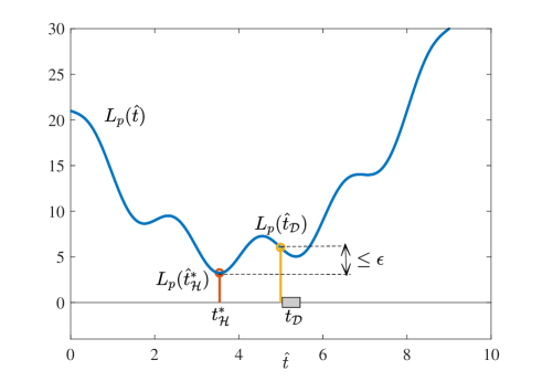
Figure 5.1: A learning algorithm $\hat{t}_{\mathcal{D}}$ outputs a hypothesis that depends on the random training set $\mathcal{D}$. It hence takes values in a given interval (the box on the horizontal axis) with some large probability $1-\delta$. The accuracy level $\epsilon$ is measured by the difference with respect to optimal generalization loss $L_{p}(\hat{t}^{*}_{\mathcal{H}})$ for the worst-case $\hat{t}_{\mathcal{D}}$ in the high-probability interval.

In order to formalize this notion, we introduce the following definition.

Definition 5.1.2.

A learning rule $\hat{t}_{\mathcal{D}}$ is ($N,\epsilon,\delta$) PAC if, when working on data sets $\mathcal{D}$ of $N$ examples, it satisfies the inequality

$$L_{p}(\hat{t}_{\mathcal{D}})\leq L_{p}(\hat{t}_{\mathcal{H}}^{*})+\epsilon$$ (5.6)

with probability no smaller than $1-\delta,$ that is,

$$\textrm{P}\textrm{r}_{\mathcal{D\underset{\textrm{i.i.d.}}{\sim}}p_{\mathrm{xt}}}[L_{p}(\hat{t}_{\mathcal{D}})\leq L_{p}(\hat{t}_{\mathcal{H}}^{*})+\epsilon]\geq 1-\delta,$$ (5.7)

for any true distribution $p(x,t)$.

In (5.6), we have defined $\epsilon$ as the accuracy parameter and $\delta$ as the confidence parameter. The accuracy is also known as estimation error or generalization gap according to the definition given in Sec. 2.3.3. In words, the ($N,\epsilon,\delta$) PAC condition (5.6) requires that the learning rule $\hat{t}_{\mathcal{D}}$ operating over $N$ data points is $\epsilon-$accurate with probability $1-\delta$ for any distribution $p(x,t)$.

The key question is: Given a model $\mathcal{H},$ how large should $N$ be in order to ensure the existence of an ($N,\epsilon$,$\delta$) PAC learning scheme $\hat{t}_{\mathcal{D}}$ for given accuracy and confidence levels $(\epsilon$,$\delta$)? At a high level, we know that a large model order implies the need for a larger $N$ in order to avoid overfitting. More precisely, we expect to observe the behavior illustrated in Fig. 5.2: As $N$ increases, (i) the interval of values taken by the generalization loss $L_{p}(\hat{t}_{\mathcal{D}})$ with probability no smaller than $1-\delta$ shrinks; and (ii) the generalization loss $L_{p}(\hat{t}_{\mathcal{D}})$ tends to the minimum generalization loss $L_{p}(\hat{t}_{\mathcal{H}}^{*}),$ and hence the estimation error vanishes. As illustrated in the next example, this expected behavior is a consequence of the law of large numbers, since a larger $N$ allows an increasingly accurate estimation of the true general loss.

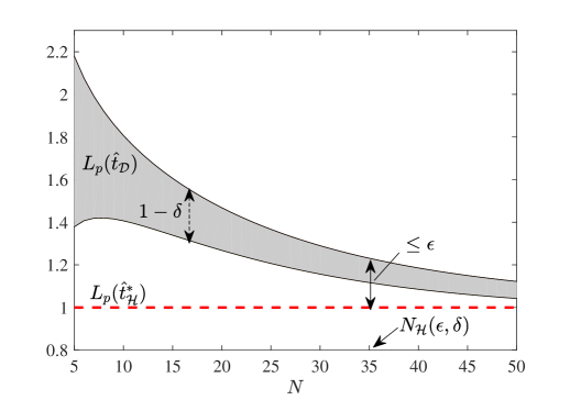
Figure 5.2: High-probability interval (dashed arrow) for the generalization error $L_{p}(\hat{t}_{\mathcal{D}})$ versus the number $N$ of data points for a model $\mathcal{H}$.

Example 5.1.3.

Consider the problem of binary classification using the model of threshold functions, namely

$$\mathcal{H}=\left\{\hat{t}_{\theta}(x)=\begin{cases}0,&\text{if }x<\theta\\ 1,&\text{if }\,x\geq\theta\end{cases}=1(x\geq\theta)\right\},$$ (5.8)

where $x$ is a real number ($D=1$). Note that the model is parametrized by the threshold $\theta$. Make the realizability assumption that the true distribution is within the hypothesis allowed by the model, i.e., $p(x,t)=p(x)1(t=\hat{t}_{0}(x))$ and hence the optimal hypothesis is $\hat{t}_{\mathcal{H}}^{*}=\hat{t}_{0}$, or, equivalently, the optimal threshold is $\theta^{*}=0$. Assuming a uniform distribution $p(x)=\mathcal{U}(x|-0.5,0.5)$ in the interval $[-0.5,0.5]$ for the domain points, Fig. 5.3 shows the generalization error $\textrm{Pr}[\hat{t}_{\theta}(\mathrm{x})\neq t_{0}(\mathrm{x})]=|\theta|$, as well as the training loss $L_{\mathcal{D}}(\hat{t}_{\theta})$ for the training set shown on the horizontal axis, for two values of $N$. Note that the training loss $L_{\mathcal{D}}(\hat{t}_{\theta})$ is simply the fraction of training examples that are correctly classified. It is observed that, as $N$ increases, the training loss, or empirical risk, becomes an increasingly reliable estimate of the generalization loss uniformly for all hypotheses, parameterized by $\theta$, in the model.

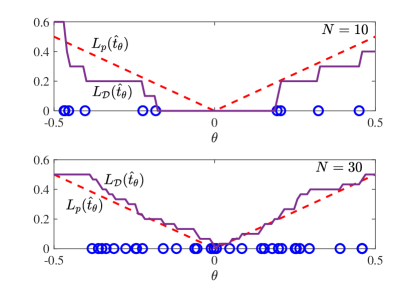
Figure 5.3: Generalization and training losses for a scalar threshold classifier model.

As suggested by the example, if $N$ is large enough, the empirical risk, or training loss, $L_{\mathcal{D}}(\hat{t})$ approximates increasingly well (with high probability) the generalization loss $L_{p}(\hat{t})$ for any fixed hypothesis in $\hat{t}\in\mathcal{H}$ by the law of large numbers. It would then seem that the problem is solved: Since $L_{\mathcal{D}}(\hat{t})\simeq L_{p}(\hat{t})$ for any $\hat{t}$, the ERM solution $\hat{t}_{\mathcal{D}}^{ERM}$, which minimizes the training loss $L_{\mathcal{D}}(\hat{t})$, should also approximately minimize the generalization loss $L_{p}(\hat{t})$, and hence we have $\hat{t}_{\mathcal{D}}^{ERM}\simeq\hat{t}_{\mathcal{H}}^{*}$. However, this argument is incorrect. In fact, we need the training loss $L_{\mathcal{D}}(\hat{t})$ to be an accurate approximation of the generalization loss $L_{p}(\hat{t})$ uniformly for all hypotheses in $\hat{t}\in\mathcal{H}$ in order to ensure the condition $\hat{t}_{\mathcal{D}}^{ERM}\simeq\hat{t}_{\mathcal{H}}^{*}.$ As we will see in the rest of this chapter, guaranteeing this condition requires to observe a number of samples $N$ that grows with the “capacity” of the model $\mathcal{H}$, that is, roughly, with the number of parameters defining the hypotheses in $\mathcal{H}$. Moreover, some models turn out to be impossible to learn – in the sense of PAC learnability formalized below – no matter how large $N$ is.

5.2 PAC Learnability and Sample Complexity

In order to formally address the key question posed above regarding the learnability of a model $\mathcal{H}$, we make the following definitions. As mentioned, for simplicity, we consider binary classification under the 0-1 loss, although the analysis can be generalized under suitable conditions [Shalev].

Definition 5.2.1.

A hypothesis class $\mathcal{H}$ is PAC learnable if, for any $\epsilon,\delta\in(0,1)$, there exist an ($N,\epsilon,\delta$) PAC learning rule as long as the inequality $N\geq N_{\mathcal{H}}(\epsilon,\delta)$ is satisfied for some function $N_{\mathcal{H}}(\epsilon,\delta)<\infty$.

In words, a hypothesis class is PAC learnable if, as long as enough data is collected, a learning algorithm can be found that obtains any desired level of accuracy and confidence. An illustration of the threshold $N_{\mathcal{H}}(\epsilon,\delta)$ can be found in Fig. 5.2. A less strong definition of PAC learnability requires (5.7) to hold only for all true distributions $p(x,t)$ that can be written as

$$p(x,t)=p(x)1(t=\hat{t}(x))$$ (5.9)

for some marginal distribution $p(x)$ and for some hypothesis $\hat{t}(x)\in\mathcal{H}$. The condition (5.9) is known as the realizability assumption, which implies that the data is generated from some mechanism that is included in the hypothesis class. Note that realizability implies the linear separability of any data set drawn from the true distribution for the class of linear predictors (see Chapter 4).

A first important, and perhaps surprising, observation is that not all models are PAC learnable. As an extreme example of this phenomenon, consider the class $\mathcal{H}$ of all functions from $\mathbb{R}^{D}$ to $\{0,1\}$. By the no free lunch theorem, this class is not PAC learnable. In fact, given any amount of data, we can always find a distribution $p(x,t)$ under which the PAC condition is not satisfied. Intuitively, even in the realizable case, knowing the correct predictor $\hat{t}(x)$ in (5.9) for any number of $x\in\mathbb{R}^{D}$ yields no information on the value of $\hat{t}(x)$ for other values of $x$. As another, less obvious, example the class

$$\mathcal{H}=\{h_{w}(x)=1(\sin(wx)>0)\}$$ (5.10)

is not PAC learnable despite being parameterized by a single scalar [Shalev].

Definition 5.2.2.

The sample complexity $N_{\mathcal{H}}^{*}(\epsilon,\delta)$ of model $\mathcal{H}$ is the minimal value of $N_{\mathcal{H}}(\epsilon,\delta)$ that satisfies the requirements of PAC learning for $\mathcal{H}$.

We will see next that the sample complexity depends on the capacity of the model $\mathcal{H}$. Note that the sample complexity of the two examples above is infinite since they are not PAC learnable. We also remark that PAC learnability may be alternatively defined under the additional conditions on the scaling of $N_{\mathcal{H}}^{*}(\epsilon,\delta)$ as a function of $\epsilon$ and $\delta$, as well as on the computational complexity of the learning rule. We will not consider these more refined definitions here, and we refer the reader to [Hastie, Shalev] for discussion.

5.3 PAC Learnability for Finite Hypothesis Classes

In this section, we consider models with a finite number of hypotheses. The main result is summarized in the following theorem, which is proved below in Sec. 5.3.1.

Theorem 5.3.1.

A finite hypothesis class $\mathcal{H}$ is PAC learnable with sample complexity satisfying the inequality

$$N_{\mathcal{H}}^{*}(\epsilon,\delta)\leq\Biggl{\lceil}\frac{2\ln|\mathcal{H}|+2\ln(2/\delta)}{\epsilon^{2}}\Biggr{\rceil}\triangleq N_{\mathcal{H}}^{ERM}(\epsilon,\delta).$$ (5.11)

Moreover, the ERM algorithm achieves the upper bound $N_{\mathcal{H}}^{ERM}(\epsilon,\delta)$.

The previous theorem shows that all finite classes are PAC learnable. Furthermore, for all finite classes, ERM is a PAC learning rule for any desired levels of accuracy and confidence ($\epsilon,\delta$), as long as $N$ is larger than the threshold $N_{\mathcal{H}}^{ERM}(\epsilon,\delta)$. This threshold, which we will refer to as the ERM sample complexity for class $\mathcal{H}$, depends on the capacity of the hypothesis class, defined as $\ln|\mathcal{H}|$ (nats) or $\log_{2}|\mathcal{H}|$ (bits). This is the number of bits required to index the hypotheses in $\mathcal{H}$. It is also interesting to note that increasing the accuracy, i.e., decreasing $\epsilon$ is more demanding than increasing the confidence, that is, decreasing $\delta$, in terms of sample complexity.

Another way to understand the result (5.11) is that, with $N$ data points, we can achieve the estimation error

$$\epsilon=\sqrt{\frac{2\ln(2|\mathcal{H}|/\delta)}{N}},$$ (5.12)

with probability $1-\delta$, by using ERM. As a result, with $N$ data points, we can upper bound the generalization loss of ERM as

$$L_{p}(\hat{t}_{\mathcal{D}}^{ERM})\leq L_{p}(\hat{t}_{\mathcal{H}}^{*})+\sqrt{\frac{2\ln|\mathcal{H}|/\delta}{N}}$$ (5.13)

with probability $1-\delta$. In words, ERM achieves the optimal generalization loss with an estimation error that scales with square root of the model capacity and with the inverse square root of $N$.

As another important note, under the realizability assumption, the theorem can be modified to yield the smaller upper bound [Shalev]

$$N_{\mathcal{H}}^{*}(\epsilon,\delta)\leq\Biggl{\lceil}\frac{\ln|\mathcal{H}|+\textrm{ln(1/}\delta)}{\epsilon}\Biggr{\rceil}\triangleq N_{\mathcal{H}}^{ERM}(\epsilon,\delta),$$ (5.14)

which is also achievable by ERM.

What does the theorem say about infinite models such as the linear classifier (5.3)? One approach is to learn a “quantized” version of $\mathcal{H},$ say $\mathcal{H}_{b}$, in which each weight is represented by $b$ bits or, equivalently, as one of $2^{b}$ pre-determined quantization levels. As a result, the number of hypotheses in the hypothesis class $\mathcal{H}$ is $|\mathcal{H}|=(2^{b})^{D+1}$, and the capacity of the hypothesis class is $\log|\mathcal{H}|=(D+1)b$ (bits) or $\ln|\mathcal{H}|=b(D+1)\ln 2$ (nats). It follows that, using (5.3), we obtain the ERM sample complexity

$$N_{\mathcal{H}}^{ERM}(\epsilon,\delta)=\Biggl{\lceil}\frac{2b(D+1)\ln 2+2\ln(2/\delta)}{\epsilon^{2}}\Biggr{\rceil}.$$ (5.15)

It is observed that the ERM sample complexity scales proportionally to the number of parameters $D+1$ and to the resolution $b$. Therefore, obtaining an arbitrary precision by selecting larger values of $b$ yields a sample complexity that grows unbounded. We will see below how to correct this result by introducing a more advanced theory of generalization through the concept of Vapnik–Chervonenkis (VC) dimension.

5.3.1 Proof of Theorem 5.3.1

The proof of Theorem 5.3.1 reveals the role played by the training loss $L_{\mathcal{D}}(\hat{t})$ in approximating the generalization loss $L_{p}(\hat{t})$ uniformly for all hypotheses $\hat{t}\in\mathcal{H}$. We start with the following key lemma.

Lemma 5.3.2.

For any $N\geq N_{\mathcal{H}}^{ERM}(\epsilon,\delta)$, we have

$$\text{Pr}_{\mathcal{D}\underset{\textrm{i.i.d.}}{\sim}p(x,t)}\left[|L_{p}(\hat{t})-L_{\mathcal{D}}(\hat{t})|\leq\frac{\epsilon}{2}\;\textrm{for all }\hat{t}\in\mathcal{H}\right]\geq 1-\delta.$$ (5.16)

Reflecting the observation made above around Fig. 5.3, the lemma says that the training loss $L_{\mathcal{D}}(\hat{t}$) is a uniformly accurate approximation, with accuracy level $\epsilon/2$, of the generalization loss, as long as $N\geq N_{\mathcal{H}}^{ERM}(\epsilon,\delta)$.

Assume now that the lemma is true – a proof will be given below. Using the lemma, Theorem 5.3.1 follows immediately from the inequalities

$$L_{p}(\hat{t}_{\mathcal{D}}^{ERM}) \leq L_{\mathcal{D}}(\hat{t}_{\mathcal{D}}^{ERM})+\frac{\epsilon}{2}\leq L_{\mathcal{D}}(\hat{t}^{*})+\frac{\epsilon}{2}$$ (5.17)

$$\leq L_{p}(\hat{t}^{*})+\frac{\epsilon}{2}+\frac{\epsilon}{2}=L_{p}(\hat{t}^{*})+\epsilon,$$ (5.18)

where the first inequality follows from the lemma; the second from the definition of ERM; and the third by another application of the lemma.

We hence only need to prove the Lemma in order to conclude the proof. To proceed, we will use Hoeffding’s inequality, which says the following (see, e.g., [Shalev]). For i.i.d. rvs $\mathrm{u}_{1},\mathrm{u}_{2},\cdots,\mathrm{u}_{M}\sim p(u)$ such that $\textrm{E}\left[\mathrm{u}_{i}\right]=\mu$ and $\textrm{Pr}[a\leq\mathrm{u}_{i}\leq b]=1$, we have the large deviation inequality

$$\text{Pr}\left[\Biggl{|}\frac{1}{M}\sum_{m=1}^{M}\mathrm{u}_{m}-\mu\Biggr{|}>\epsilon\right]\leq 2\exp\left(-\frac{2M\epsilon^{2}}{(b-a)^{2}}\right).$$ (5.19)

We can now write the following sequence of equalities and inequalities, which prove the lemma and hence conclude the proof:

$$\text{Pr}_{\mathcal{D}\underset{\textrm{i.i.d.}}{\sim}p(x,t)}\left[\exists\hat{t}\in\mathcal{H}:\textrm{}|L_{p}(\hat{t})-L_{\mathcal{D}}(\hat{t})|>\frac{\epsilon}{2}\right]$$

$$= \text{Pr}_{\mathcal{D}\underset{\textrm{i.i.d.}}{\sim}p(x,t)}\left[\bigcup_{\hat{t}\in\mathcal{H}}\left\{|L_{p}(\hat{t})-L_{\mathcal{D}}(\hat{t})|>\frac{\epsilon}{2}\right\}\right]$$

$$\leq \sum_{\hat{t}\in\mathcal{H}}\text{Pr}_{\mathcal{D}\underset{\textrm{i.i.d.}}{\sim}p(x,t)}\left[|L_{p}(\hat{t})-L_{\mathcal{D}}(\hat{t})|>\frac{\epsilon}{2}\right]$$

$$\underset{}{\leq} 2\sum_{\hat{t}\in\mathcal{H}}\exp\left(-\frac{N\epsilon^{2}}{2}\right)$$

$$= 2|\mathcal{H}|\exp\left(-\frac{N\epsilon^{2}}{2}\right)\leq\delta,$$

where the first inequality follows by the union bound; the second by Hoeffding’s inequality; and the third can be verified to be true as long as the inequality $N\geq N_{\mathcal{H}}^{ERM}(\epsilon,\delta)$ is satisfied.

5.3.2 Structural Risk Minimization^∗

The result proved above is useful also to introduce the Structural Risk Minimization (SRM) learning approach. SRM is a method for joint model selection and hypothesis learning that is based on the minimization of an upper bound on the generalization loss. In principle, the approach avoids the use of validation, and has deep theoretical properties in terms of generalization [Shalev]. In practical applications, the approach is rarely used, and validation is often preferable. It is nevertheless conceptually and theoretically a cornerstone of statistical learning theory.

To elaborate, assume that we have a nested set of hypothesis classes $\mathcal{H}_{1}\subseteq\mathcal{H}_{2}\subseteq...\subseteq\mathcal{H}_{M_{\max}}$. For instance, the nested model may correspond to linear classifiers with increasing orders $M\in\{1,2,...,M_{\max}\}$. From Lemma 5.3.2, we can obtain the following bound

$$L_{p}(\hat{t})\leq L_{\mathcal{D}}(\hat{t})+\sqrt{\frac{\ln(2|\mathcal{H}_{M}|/\delta)}{2N}}$$ (5.20)

for all $\hat{t}\in\mathcal{H}_{M},\text{ with probability }1-\delta.$ SRM minimizes this upper bound, which is a pessimistic estimate of the generalization loss, over both the choice of the model $M$ and the hypothesis $\hat{t}\in\mathcal{H}_{M}$. We note the similarity of this approach with the simplified MDL criterion based on two-part codes covered in Chapter 2.

5.4 VC Dimension and Fundamental Theorem of PAC Learning

We have seen that finite classes are PAC learnable with sample complexity proportional to the model capacity $\ln|\mathcal{H}|$ by using ERM. In this section, we address the following questions: Is $N_{\mathcal{H}}^{ERM}(\epsilon,\delta)$ the smallest sample complexity? How can we define the capacity of infinite hypothesis classes? We have discussed at the end of Sec. 5.3 that the answer to the latter question cannot be found by extrapolating from results obtained when considering finite hypothesis classes. In contrast, will see here that the answers to both of these questions rely on the concept of VC dimension, which serves as a more fundamental definition of capacity of a model. The VC dimension is defined next.

Definition 5.4.1.

A hypothesis class $\mathcal{H}$ is said to shatter a set of domain points $\mathcal{X}=\{x_{n}\}_{n=1}^{V}$ if, no matter how the corresponding labels $\{t_{n}\in\{0,1\}\}_{n=1}^{V}$ are selected, there exists a hypothesis $\hat{t}\in\mathcal{H}$ that ensures $\hat{t}(x_{n})=t_{n}$ for all $n=1,...,V$.

Definition 5.4.2.

The VC dimension $\text{VCdim}(\mathcal{H})$ of the model $\mathcal{H}$ is the size of the largest set $\mathcal{X}$ that is shattered by $\mathcal{H}.$

Based on the definitions above, to prove that a model has $\text{VCdim}(\mathcal{H})=V$, we need to carry out the following two steps:

Step 1) Demonstrate the existence of a set $\mathcal{X}$ with $|\mathcal{X}|=V$ that is shattered by $\mathcal{H}$; and

Step 2) Prove that no set $\mathcal{X}$ of dimension $V+1$ exists that is shattered by $\mathcal{H}$.

The second step is typically seen to be more difficult, as illustrated by the following examples.

Example 5.4.3.

The threshold function model (5.8) has VCdim($\mathcal{H}$)$=1$, since there is clearly a set $\mathcal{X}$ of one sample ($V=1$) that can be shattered (Step 1); but there are no sets of $V=2$ that can be shattered (Step 2). In fact, for any set $\mathcal{X}=(x_{1},x_{2})$ of two points with $x_{1}\leq x_{2}$, the label assignment $(t_{1},t_{2})=(1,0)$ cannot be realized by any choice of the threshold $\theta$, which is the only parameter in the model.

Example 5.4.4.

The model $\mathcal{H}=\{\hat{t}_{a,b}(x)=1\left(a\leq x\leq b\right)\}$, which assigns the label $t=1$ within an interval $[a,b]$ and the label $t=0$ outside it, has VCdim($\mathcal{H}$)$=2$. In fact, any set of $V=2$ points can be shattered – and hence there also exists one such set (Step 1); while there are no sets $\mathcal{X}$ of $V=3$ points that can be shattered (Step 2). For Step 2, note that, for any set $\mathcal{X}=(x_{1},x_{2},x_{3})$ of three points with $x_{1}\leq x_{2}\leq x_{3}$, the label assignment $(t_{1},t_{2},t_{3})=(1,0,1)$ cannot be realized by any choice of the two free parameters $(a,b)$.

Example 5.4.5.

The model $\mathcal{H}=\{\hat{t}_{a_{1},a_{2},b_{1},b_{2}}(x)=1(a_{1}\leq x_{1}\leq a_{2}\;\text{and}\;b_{1}\leq x_{2}\leq b_{2})\}$, which assigns the label $t=1$ within an axis-aligned rectangle defined by parameters $a_{1},a_{2},b_{1}$ and $b_{2}$ has VCdim($\mathcal{H}$)$=4$, as it can be proved by using arguments similar to the previous examples.

Example 5.4.6.

The linear classifier (5.3) has VCdim($\mathcal{H}$)$=D+1$ [Shalev].

The example above suggests that the VC dimension of a set often coincides with the number of degrees of freedom, or free parameters, in the model. However, this is not necessarily the case.

Example 5.4.7.

Model (5.10), while having a single parameter, has an infinite VC dimension [Shalev].

We also note that, for finite classes, we have the inequality $\text{VCdim}(\mathcal{H})\leq\log|\mathcal{H}|$, since $|\mathcal{H}|$ hypotheses can create at most $|\mathcal{H}|$ different label configurations. The next theorem, whose importance is attested by its title of fundamental theorem of PAC learning, provides an answer to the two questions posed at the beginning of this section.

Theorem 5.4.8.

A model $\mathcal{H}$ with finite VCdim($\mathcal{H}$)$=d<\infty$ is PAC learnable with sample complexity

$$C_{1}\frac{d+\ln(1/\delta)}{\epsilon^{2}}\leq N_{\mathcal{H}}^{*}(\epsilon,\delta)\leq C_{2}\frac{d+\ln(1/\delta)}{\epsilon^{2}}$$ (5.21)

for some constants $C_{1}$ and $C_{2}$. Moreover, the ERM learning rule achieves the upper bound.

The theorem shows that the sample complexity is proportional to $(\textrm{VCdim}(\mathcal{H})+\ln(1/\delta))/\epsilon^{2}$. This reveals that VCdim($\mathcal{H}$) can be considered as the correct definition of capacity for a hypothesis class $\mathcal{H}$, irrespective of whether the class is finite or not: As VCdim($\mathcal{H}$) increases, the number of required data points for PAC learning increases proportionally to it. Furthermore, the theorem demonstrates that, if learning is possible for a given model $\mathcal{H},$ then ERM allows us to learn with close-to-optimal sample complexity.

For a proof of this result and for extensions, we refer to the extensive treatment in [Shalev]. We mention here the important extension of the theory of generalization to convex learning problems – i.e., to problems with convex parameter set and a convex loss function. Rather than depending on the model complexity as the theory developed so far, generalization in this class of problems hinges on the stability of the learning algorithms. Stability is the property that small changes in the input do not affect much the output of the learning algorithm – a notion related to that of differential privacy [raginsky2016information]. We also point to the related notion of capacity of a perceptron introduced in [Mackay].

5.5 Summary

This chapter has described the classical PAC framework for the analysis of the generalization performance of supervised learning for classification. We have seen that the concept of VC dimension defines the capacity of the model, and, through it, the number of samples needed to learn the model with a given accuracy and confidence, or sample complexity. In the next chapter, we move from supervised learning to unsupervised learning problems.

Appendix: Minimax Redundancy and Model Capacity^∗

In this appendix, we describe an alternative definition of model capacity that is directly related to the conventional notion of Shannon’s capacity of a noisy channel [Cover]. As for Sec. 2.5, some background in information theory may be needed to fully appreciate the content of this appendix.

To elaborate, consider a probabilistic model $\mathcal{H}$ defined as the set of all pmfs $p(x|\theta)$ parametrized by $\theta$ in a given set. With some abuse of notation, we take $\mathcal{H}$ to be also the domain of parameter $\theta$. To fix the ideas, assume that $x$ takes values over a finite alphabet. We know from Sec. 2.5, that a distribution $q(x)$ is associated with a lossless compression scheme that requires around $-\log q(x)$ bits to describe a value $x$. Furthermore, if we were informed about the true parameter $\theta$, the minimum average coding length would be the entropy $H(p(x|\theta)),$ which requires setting $q(x)=p(x|\theta)$ (see Appendix A).

Assume now that we only know that the parameter $\theta$ lies in set $\mathcal{H}$, and hence the true distribution $p(x|\theta)$ is not known. In this case, we cannot select the true parameter distribution, and we need instead to choose a generally different distribution $q(x)$ to define a compression scheme. With a given distribution $q(x)$, the average coding length is given by $-\sum_{x}p(x|\theta)\log q(x)$. Therefore, the choice of a generally incorrect distribution $q(x)$ entails a redundancy of

$$\Delta R(q(x),\theta)=-\sum_{x}p(x|\theta)\log q(x)-H(p(x|\theta))\geq 0$$ (5.22)

bits.

The redundancy $\Delta R(q(x),\theta)$ in (5.22) depends on the true value of $\theta$. Since the latter is not known, this quantity cannot be computed. We can instead obtain a computable metric by maximizing over all values of $\theta\in\mathcal{H}$, which yields the worst-case redundancy

$$\Delta R(q(x),\mathcal{H})=\underset{\theta\in\mathcal{H}}{\textrm{ }\max}\Delta R(q(x),\theta).$$ (5.23)

This quantity can be minimized over $q(x)$ yielding the so-called minimax redundancy:

$$\Delta R(\mathcal{H}) =\underset{q(x)}{\min}\Delta R(q(x),\mathcal{H})$$ (5.24)

$$=\underset{q(x)}{\min}\underset{\theta}{\textrm{ }\max}-\sum_{x}p(x|\theta)\log q(x)-H(p(x|\theta))$$ (5.25)

$$=\underset{q(x)}{\min}\underset{\theta}{\textrm{ }\max}\sum_{x}p(x|\theta)\log\frac{p(x|\theta)}{q(x)}.$$ (5.26)

The minimax redundancy can be taken as a measure of the capacity of model $\mathcal{H},$ since a richer model tends to yield a larger $\Delta R(\mathcal{H}).$ In fact, for a richer model, it is more difficult to find a representative distribution $q(x)$ that yields an average coding length close to the minimum $H(p(x|\theta))$ for all values of $\theta$.

It turns out that the minimax redundancy equals the capacity $C(p(x|\theta))$ of the channel $p(x|\theta)$, which is defined as $C(p(x|\theta))=\max_{p(\theta)}I(\mathrm{x};\text{$\mathrm{\theta}$})$ [Cover]. This is shown by the following sequence of equalities:

$$\Delta R(\mathcal{H})= \underset{q(x)}{\min}\underset{p(\theta)}{\textrm{ }\max}\sum_{x}\sum_{\theta}p(\theta)p(x|\theta)\log\frac{p(x|\theta)}{q(x)}$$ (5.27a)

$$= \underset{p(\theta)}{\max}\underset{q(x)}{\textrm{ }\min}\sum_{x}\sum_{\theta}p(\theta)p(x|\theta)\log\frac{p(x|\theta)}{q(x)}$$ (5.27b)

$$= \underset{p(\theta)}{\max}\sum_{x}\sum_{\theta}p(\theta)p(x|\theta)\log\frac{p(x|\theta)}{p(x)}$$ (5.27c)

$$= C(p(x|\theta)),$$ (5.27d)

where the first equality follows since the average of a set of numbers is no larger than any of the numbers; the second is a consequence of the minimax theorem since the term $\sum_{x}\sum_{\theta}p(\theta)p(x|\theta)\log(p(x|\theta)/q(x))$ is convex in $q(x)$ and concave in $p(\theta)$; and the third equality follows by Gibbs’ inequality (see Sec. 2.6 and (A.5) in Appendix A). As a final note, the mutual information $I(\mathrm{x};\text{$\mathrm{\theta}$})$ between model parameter and data also plays a central role in obtaining bounds on the performance of estimation [loh2017lower].

Part III Unsupervised Learning

Chapter 6 Unsupervised Learning

Unlike supervised learning, unsupervised learning tasks operate over unlabelled data sets. Apart from this general statement, unsupervised learning is more loosely defined than supervised learning, and it also lacks a strong theoretical framework to mirror the PAC learning theory covered in the previous chapter. Nevertheless, it is widely expected that future breakthroughs in machine learning will come mainly from advances in the theory and design of unsupervised learning algorithms. This is due to the availability of huge repositories of unlabelled data, as well as to the broader applicability of learning tasks whereby the machine learns, as it were, without supervision or feedback. Unsupervised learning is also considered by some as the key to the development of general, as opposed to task, specific AI [spectrumlc] (see also [Tegmark, Levesque17] for more on general AI).

Generally speaking, unsupervised learning algorithms aim at learning some properties of interest of the mechanism underlying the generation of the data. In this sense, unsupervised learning concerns the study of generative models, although, as we will see, this statement comes with some caveats. A common aspect of many models used for unsupervised learning is the presence of hidden, or latent, variables that help explain the structure of the data.

This chapter starts by discussing applications of unsupervised learning, and by providing a description of the well-known $K$-means algorithm. It then covers directed and undirected generative probabilistic models for unsupervised learning. As we will detail, these models posit different types of statistical dependence relations between hidden and measured variables. Discriminative models, which capture the dependence of hidden variables on observed variables, as well as autoencoders, which combine discriminative and generative models, are also introduced. The chapter is concluded with a discussion of a different type of learning algorithm that may be considered as unsupervised, namely PageRank, which is included due to its practical relevance.

6.1 Unsupervised Learning

Defining unsupervised learning. A general, and rather imprecise, definition of unsupervised learning tasks is the following. Taking a frequentist viewpoint, we are given a data set $\mathcal{D}$ consisting of $N$ i.i.d. unlabelled observations $\mathrm{x}_{n}\in\bm{\mathbb{R}}^{D}$. These are assumed to be drawn i.i.d. from an unknown true distribution as

$$\mathcal{D}=\{\mathrm{x}_{n}\}_{n=1}^{N}\underset{\text{i.i.d.}}{\sim}p(x).$$ (6.1)

The goal is to learn some useful properties of the distribution $p(x)$, where the properties of interest depend on the specific application. While this definition is general enough to include also the estimation problems studied in Chapter 3, as mentioned, unsupervised learning problems are typically characterized by the presence of hidden or latent variables. Notable examples include the following.

$\bullet$ Density estimation: Density estimation aims at learning directly a good approximation of the distribution $p(x)$, e.g., for use in plug-in estimators [lehmann2006theory], to design compression algorithms (see Sec. 2.5), or to detect outliers [outliers].

$\bullet$ Clustering: Clustering assumes the presence of an unobserved label $z_{n}$ associated to each data point $x_{n}$, and the goal is that of recovering the labels $z_{n}$ for all points in the data set $\mathcal{D}.$ For example, one may wish to cluster a set $\mathcal{D}$ of text documents according to their topics, by modelling the latter as an unobserved label $z_{n}$. Broadly speaking, this requires to group together documents that are similar according to some metric. It is important at this point to emphasize the distinction between classification and clustering: While the former assumes the availability of a labelled set of training examples and evaluates its (generalization) performance on a separate set of unlabelled examples, the latter works with a single, unlabelled, set of examples. The different notation used for the labels – $z_{n}$ in lieu of $t_{n}$ – is meant to provide a reminder of this key difference.

$\bullet$ Dimensionality reduction and representation: Given the set $\mathcal{D}$, we would like to represent the data points $x_{n}\in\mathcal{D}$ in a space of lower dimensionality. This makes it possible to highlight independent explanatory factors, and/or to ease visualization and interpretation [visualization], e.g., for text analysis via vector embedding (see, e.g., [Rudolphemb]).

$\bullet$ Feature extraction: Feature extraction is the task of deriving functions of the data points $x_{n}$ that provide useful lower-dimensional inputs for tasks such as supervised learning. The extracted features are unobserved, and hence latent, variables. As an example, the hidden layer of a deep neural network extract features from the data for use by the output layer (see Sec. 4.5).

$\bullet$ Generation of new samples: The goal here is to learn a machine that is able to produce samples that are approximately distributed according to the true distribution $p(x)$. For example, in computer graphics for filmmaking or gaming, one may want to train a software that is able to produce artificial scenes based on a given description.

The variety of tasks and the difficulty in providing formal definitions, e.g., on the realism of an artificially generated image, make unsupervised learning, at least in its current state, a less formal field than supervised learning. Often, loss criteria in unsupervised learning measure the divergence between the learned model and the empirical data distribution, but there are important exceptions, as we will see.

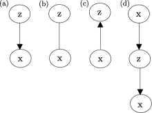
Figure 6.1: (a) Directed generative models; (b) Undirected generative models; (c) Discriminative models; (d) Autoencoders.

Models. We now review the type of models that can be used to tackle unsupervised learning problems. The models will be further discussed in the subsequent sections of this chapter.

$\bullet$ Directed generative models: Directed generative models are mixture models in which the distribution $p(x|\theta)$ of the data is defined by a parametrized prior $p(z|\theta)$ of the latent variables $\mathrm{z}$ and by a parametrized conditional distribution $p(x|z,\theta)$ that defines the relationship between latent and observed variables. Accordingly, the distribution can be expressed, for discrete latent variables $\mathrm{z}$, as

$$p(x|\theta)=\sum_{z}p(z|\theta)p(x|z,\theta).$$ (6.2)

A similar expression applies to continuous hidden variables with an integral in lieu of the sum. Directed models are suitable to capture the cause-effect relationships between $\mathrm{z}$ and $\mathrm{x}$. A BN describing directed generative models is shown in Fig. 6.1(a). Graphical models, including BNs, will be covered in detail in the next chapter. Examples of directed generative models include the mixture of Gaussians model, and the so-called likelihood-free models, in which the conditional distribution $p(x|z,\theta)$ is implemented by a deterministic transformation, most typically a multi-layer network.

$\bullet$ Undirected generative models: Undirected models parametrize directly the joint distribution of the observed variables $\mathrm{x}$ and the hidden variables $\mathrm{z}$ as $p(x,z|\theta)$, and accordingly write the distribution of the data as

$$p(x|\theta)=\sum_{z}p(x,z|\theta).$$ (6.3)

Unlike directed models, undirected models capture the affinity, or compatibility, of given configurations of values for $\mathrm{z}$ and $\mathrm{x}$. An Markov Random Field (MRF) describing undirected generative models is shown in Fig. 6.1(b) (see next chapter). A prominent example is given by RBMs.

$\bullet$ Discriminative models: Discriminative models attempt to directly learn an encoding probabilistic mapping $p(z|x,\theta)$ between the data point $\mathrm{x}$ and a representation $\mathrm{z}.$ This is represented by the BN in Fig. 6.1(c).

$\bullet$ Autoencoders: As seen in Fig. 6.1(d), autoencoders compose a parametrized discriminative model $p(z|x,\theta)$, which produces the hidden variables $\mathrm{z}$ from the data $\mathrm{x}$, with a parametrized generative model $p(x|z,\theta).$ The former is known as encoder, while the latter as decoder. Accordingly, the latent variables are also referred to as the code. The most typical implementations use parameterized deterministic functions $z=F_{\theta}(x)$ and $x=G_{\theta}(z)$ in lieu of the more general probabilistic models $p(z|x,\theta)$ and $p(x|z,\theta)$, respectively. As we will see, autoencoders are trained to reproduce the data $x$ at the output, turning the unsupervised problem into a supervised one with “labels” given by the data point $x$ itself.

6.2 $K$-Means Clustering

We start by reviewing the well-known $K$-means clustering algorithm. The purpose here is to emphasize an algorithmic structure, namely the Expectation Maximization (EM) algorithm, that is conceptually at the core of many unsupervised learning algorithms.

The problem is one of multi-cluster clustering: Given a data set $\mathcal{D}=\{x_{n}\}_{n=1}^{N}$, we would like to assign every vector $x_{n}\in\mathbb{R}^{D}$ to one of $K$ clusters. Cluster indices are encoded by categorical variables $z_{n}$ via one-hot encoding (see Chapter 3). Accordingly, we write the $k$th component of vector $z_{n}$ as $z_{kn}=1$ if $x_{n}$ is assigned to cluster $k$, while we write $z_{kn}=0$ otherwise. It is emphasized that the labels are not given for any of the examples in $\mathcal{D}$. Therefore, the algorithm should discern some regularity in the data in order to divide the data set into $K$ classes.

$K$-means is a heuristic method that attempts to cluster together points that are mutually close in Euclidean distance. To this end, $K$-means assigns all points in the same cluster a given “prototype” representative vector $\mu_{k}$. This vector can be thought of in terms of quantization: all points within a given cluster can be quantized to the prototype $\mu_{k}$ with minimal quadratic loss. This is formalized by the following optimization problem over the cluster assignment variables $z_{n}$ and the cluster representatives $\mu_{k}$:

$$\underset{\{z_{n}\},\{\mu_{k}\}}{\textrm{min}}{\displaystyle\sum_{n=1}^{N}}\sum_{k=1}^{K}z_{kn}d(x_{n},\mathbf{\mu}_{k}),$$ (6.4)

where $d(x,\mathbf{\mu})=\left\|x-\mathbf{\mu}\right\|^{2}$ is the squared Euclidean distance. When using a general distance metric, the approach to be described is instead known as the $K$-medoids algorithm. In this regard, we note, for instance, that it is possible to apply clustering also to discrete data as long as the distance $d$ is properly defined – typically by a matrix of pairwise dissimilarities.

The $K$-means algorithm performs alternatively optimization of the cluster assignment variables $z_{n}$ and of the cluster representatives $\mu_{k}$ as follows:

$\bullet$ Initialize cluster representatives $\{\mu_{k}^{\textrm{old}}\}.$

$\bullet$ Expectation step, or E step: For fixed vectors $\{\mu_{k}^{\textrm{old}}\},$ solve problem (6.4) over the cluster assignment $\{z_{n}\}$:

$$z_{kn}^{\textrm{new}}=\begin{cases}1&\textrm{for }k=\text{$\textrm{argmin}_{j}$ }d(x_{n},\mu{}_{j}^{\textrm{old}})\\ 0&\text{otherwise}\end{cases}.$$ (6.5)

Accordingly, each training point is assigned to the cluster with the closest prototype. Note that this step generally requires the computation of $K$ distances for each data point $x_{n}$.

$\bullet$ Maximization step, or M step: For fixed vectors $\{z_{n}\}$, solve problem (6.4) over the cluster representatives $\{\mu_{k}\}$. Imposing the optimality condition that the gradient of the objective function in (6.4) be zero, we obtain

$$\mu_{k}^{\text{new}}=\frac{\sum_{n=1}^{N}z_{kn}^{\text{new}}x_{n}}{\sum_{n=1}^{N}z_{kn}^{\text{new}}}.$$ (6.6)

The new cluster representative $\mu_{k}^{\text{new}}$ for each cluster $k$ is the mean of the data points assigned to cluster $k$.

$\bullet$ If a convergence criterion is not satisfied, set {$\mu_{k}^{\text{old}}\}\leftarrow\{\mu_{k}^{\text{new}}\}$ and return to the E step.

Since both E step and M step minimize the objective function in (6.4), respectively over the cluster assignment variables $z_{n}$ and the cluster representatives $\mu_{k}$, the value of the objective function is non-decreasing across the iterations. This ensures convergence. Illustrations of convergence and examples can be found in [Bishop, Chapter 9]. As a note, the algorithm is also known as Lloyd-Max quantization [Gray].

At a high level, $K$-means alternates between: (i) making inferences about the hidden variables {$z_{n}$} based on the current model defined by the representatives {$\mu_{k}$} in the E step; and (ii) updating the model {$\mu_{k}$} to match the data {$x_{n}$} and the inferred variables {$z_{n}$} in the M step. We will see that a similar algorithmic structure is applied by many unsupervised learning algorithms.

Before we move on to discussing more general solutions, it is worth spending a few words on the problem of selecting the number $K$ of clusters. A first possibility is to add or remove clusters until certain heuristic criteria are satisfied, such as the “purity” of clusters. A second approach is hierarchical clustering, whereby one builds a tree, known as dendrogram, that includes clustering solutions with an increasing number of clusters as one moves away from the root (see, e.g., [Hastie]). Yet another solution is to let $K$ be selected automatically by adopting a non-parametric Bayesian approach via a Dirichlet process prior [Murphy].

6.3 ML, ELBO and EM

In this section, we discuss two key technical tools that are extensively used in tackling unsupervised learning problems, namely the Evidence Lower BOund (ELBO) and the EM algorithm. The starting point is the fundamental problem of learning a probabilistic, directed or undirected, model $p(x|\theta)$ from the data using ML. We will discuss later how to learn discriminative models and autoencoders.

6.3.1 ML Learning

From Sec. 2.6, we know that ML, asymptotically in $N$, tends to minimize a KL divergence between the true distribution $p(x)$ and the selected hypothesis in the model. This is a criterion that is well suited for many of the unsupervised learning tasks mentioned above, such as density estimation or generation of new samples, and it is hence useful to start the discussion with ML learning.

Before we do that, a few remarks are in order. First, it is often useful to choose divergences other than KL, which are tailored to the specific application of interest [Wasserstein]. We will further discuss this aspect in Sec. 6.4.3. Second, when the goal is representation learning, the machine aims at obtaining useful features $z$. Hence, minimizing the KL divergence to match the true distribution $p(x)$ does not directly address the objective of representation learning, unless appropriate restrictions are imposed on the model $p(x|z,\theta).$ In fact, if the generative model $p(x|z,\theta)$ is too powerful, then it can disregard the features $\mathrm{z}$ and still obtain a high likelihood for the data (see, e.g., [blogMLuns]). We will get back to this point in Sec. 6.6. Finally, obtaining ML solutions is often impractical, particularly in large models. Nevertheless, understanding the ML problem allows one to better gauge the impact of the approximations and simplifications made to obtain efficient algorithms.

To proceed, we consider probabilistic, directed or undirected, model, and focus, for the purpose of simplifying the notation, on a data set with a single data point ($N=1$). The extension to a data set with an arbitrary number $N$ of points only requires adding an outer sum over the sample index to the LL function. We also concentrate on discrete hidden rvs, and the generalization to continuous rvs is obtained by substituting sums with suitable integrals. The ML problem can be written as the maximization of the LL function as

$$\underset{\theta}{\text{max }}\ln p(x|\theta)=\ln\left(\sum_{z}p(x,z|\theta)\right),$$ (6.7)

where $x$ denotes the data and $z$ the hidden or latent variables. Note the marginalization with respect to the hidden variables in (6.7). This problem should be contrasted with the supervised learning ML problem obtained when both $x$ and $z$ are observed, namely

$$\underset{\theta}{\text{max }}\ln p(x,z|\theta).$$ (6.8)

Example 6.3.1.

Consider a directed generative Bernoulli-Gaussian model characterized as

$$\mathrm{z}\sim\textrm{Bern}(0.5)$$ (6.9a)

$$\mathrm{x}|\mathrm{z}=0\sim\mathcal{N}(2,1)$$ (6.9b)

$$\mathrm{x}|\mathrm{z}=1\sim\mathcal{N}(\theta,1).$$ (6.9c)

This corresponds to a mixture of Gaussians model, in which the only parameter $\theta$ is the mean of one of the two Gaussian components. Assume that we observe $x=0$. Consider first the supervised learning case, where we assume that we also measure $z=1$. In this case, the LL function in (6.8) is $\ln p(x=0,z=1|\theta)=\ln\mathcal{N}(x|\theta,1)+\textrm{$\ln(0.5)$}.$ In contrast, with unsupervised learning, the LL function in (6.7) is $\ln p(x=0|\theta)=\ln(0.5\mathcal{N}(0|2,1)+0.5\mathcal{N}(0|\theta,1))$.

The LL functions are shown in Fig. 6.2. Unlike supervised learning, the LL for unsupervised learning is seen to be non-concave. In this example, this is a consequence of the fact that, when $\theta$ is sufficiently large in absolute value, the probability of the data $x$ resulting from the fixed Gaussian distribution centered at $x=2$ makes the contribution of the Gaussian centered $\theta$ increasingly irrelevant.

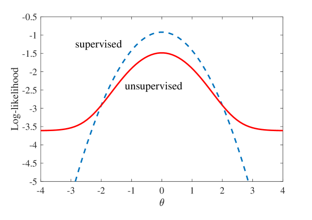
Figure 6.2: Illustration of LL functions for supervised and unsupervised learning in a mixture of Gaussians model (Example 6.3.1).

Solving problem (6.7) has two additional complications as compared to the supervised learning counterpart (6.8). The first issue was highlighted in the previous example: Even for models in which the ML supervised learning problem is convex, the LL is generally non-concave when the variables $\mathrm{z}$ are hidden, which precludes the use of convex optimization algorithms. Barring the use of often impractical global optimization algorithms, in general, non-convex problems cannot be solved exactly. Rather, the best one can hope for with standard local optimization schemes, such as SGD, is obtaining stationary points or locally optimal points [Boyd]. In practice, this problem may not be critical since non-convexity is not by itself a cause of poor learning performance. For instance, as seen in Chapter 4, beyond-GLM supervised learning methods, including deep neural networks, solve non-convex problems.

The second complication is the need to sum – or integrate – over the hidden variables in order to evaluate the LL. This step is complicated by the fact that the distribution of the hidden variables needs to be learned and is hence unknown. This is a significant obstacle to the development of efficient learning algorithms, and it generally needs to be addressed in order to make learning feasible. In the rest of this section, we describe two technical tools that are useful to tackle these problems. Chapter 8 will develop more complex solutions for issues arising in the presence of large latent spaces in which marginalization is not viable.

6.3.2 ELBO

Many methods to tackle the ML problem (6.7) are based on the maximization of the ELBO. These techniques include the EM algorithm and some of the variational inference algorithms to be discussed in Chapter 8. The key element in the development of the ELBO is the introduction of an auxiliary distribution $q(z)$ on the latent variables. This is referred to as the variational distribution or the variational posterior for reasons that will be made clear later. As we will see, computation of the ELBO requires an average over distribution $q(z)$, which can be fixed independently of the model parameters. This solves the key problem identified above of averaging over the parameter-dependent marginal of the hidden variables.

Definition 6.3.2.

For any fixed value $x$ and any distribution $q(z)$ on the latent variables $\mathrm{z}$ (possibly dependent on $x$), the ELBO $\mathcal{L\mathrm{(\text{$q$},\theta)}}$ is defined in one of the following equivalent forms

$$\mathcal{L}(q,\theta)= \textrm{E}_{\mathrm{z}\sim q(z)}[\underbrace{\ln p(x,\mathrm{z}|\theta)-\ln q(\mathrm{z})}_{\textrm{learning signal}}]$$ (6.10)

$$= \underbrace{\textrm{E}_{\mathrm{z}\sim q(z)}[\ln p(x,\mathrm{z}|\theta)]}_{\text{negative energy }}+\underbrace{H(q)}_{\text{entropy }}$$ (6.11)

$$= \underbrace{\textrm{E}_{\mathrm{z}\sim q(z)}[\ln p(x|\mathrm{z},\theta)]}_{\textrm{cross-entropy}}-\underbrace{\text{KL}\left(q(z)||p(z|\theta)\right)}_{\textrm{variational regularization}}$$ (6.12)

$$= -\text{KL}\left(q(z)||p(x,z|\theta)\right)$$ (6.13)

$$= \ln p(x|\theta)-\text{KL}\left(q(z)||p(z|x,\theta)\right),$$ (6.14)

where we have identified some terms using common terminology that will be clarified in the following, and, in (6.13), we have used the convention of defining $\text{KL}(p||q)$ even when $q$ is not normalized (see Sec. 2.6).

The equivalence between the three forms of the ELBO can be easily checked. The form (6.11) justifies the definition of the negative of the ELBO as variational free energy or Gibbs free energy, which is the difference of energy and entropy. This form is particularly useful for undirected models in which one specifies directly the joint distribution $p(x,z|\theta)$, such as energy-based models, while the form (6.12) is especially well suited for directed models that account for the discriminative distribution $p(x|z,\theta)$, such as for deep neural networks [blundell2015weight]. For both forms the first term can be interpreted as a cross-entropy loss. The form (6.13) is more compact, and suggests that, as we will formalize below, the ELBO is maximized when $q(z)$ is selected to match the model distribution. The last form yields terms that are generally not easily computable, but it illuminates the relationship between the LL function and the ELBO, as we discuss next.

The following theorem describes the defining property of the ELBO as well as another important property. Taken together, these features make the ELBO uniquely suited for the development of algorithmic solutions for problem (6.7).

Theorem 6.3.3.

The ELBO is a global lower bound on the LL function, that is,

$$\text{$\ln p(x|$$\theta$) }\geq\mathcal{L}(q,\theta),$$ (6.15)

where equality holds at a value $\theta_{0}$ if and only if the distribution $q(z)$ satisfies $q(z)=p(z|x,\theta_{0})$. Furthermore, the ELBO is concave in $q(z)$ for a fixed $\theta$; and, if $\ln p(x,z|\theta)$ is concave in $\theta$, it is also concave in $\theta$ for a fixed $q(z)$.

Proof 6.3.4.

The first part of the theorem follows immediately from the form (6.14), which we can rewrite as

$$\ln p(x|\theta)=\text{$\mathcal{L}$$(q,\theta)+$KL}\left(q(z)||p(z|x,\theta)\right),$$ (6.16)

and from Gibbs’ inequality. In fact, the latter implies that the KL divergence $\text{KL}\left(q(z)||p(z|x,\theta)\right)$ is non-negative and equal to zero if and only if the two distributions in the argument are equal. The concavity of the ELBO can be easily checked using standard properties of convex functions [Boyd]. As a note, an alternative proof of the first part of the theorem can be provided via the importance sampling trick and Jensen’s inequality. In fact, we can write

$$\ln p(x|\theta)= \ln\left(\sum_{z}p(x,z|\theta)\right)$$ (6.17a)

$$= \ln\left(\sum_{z}q(z)\frac{p(x,z|\theta)}{q(z)}\right)$$ (6.17b)

$$\underset{}{\geq} \sum_{z}q(z)\ln\left(\frac{p(x,z|\theta)}{q(z)}\right)=\mathcal{L}(q,\theta),$$ (6.17c)

where the first equality is just obtained by multiplying and dividing by $q(z)$ – the importance sampling trick – and the last step is a consequence of Jensen’s inequality. We recall that Jensen’s inequality says that for any concave function $f(x)$ – here $f(x)=\ln(x)$ – we have the inequality $\textrm{E}[f(\mathrm{x})]\leq f(\textrm{E}[\mathrm{x}])$.

We illustrate the just described properties of the ELBO via the following example.

Example 6.3.5.

Consider again the directed generative Bernoulli-Gaussian model (6.9). The posterior distribution of the latent variable given an observation $x$ is given as

$$p(z=1|x=0,\theta)=\frac{\mathcal{N}(0|\theta,1)}{\mathcal{N}(0|2,1)+\mathcal{N}(0|\theta,1)}.$$ (6.18)

Fix a parametrized variational distribution $q(z|\varphi)=\textrm{Bern$(z|\varphi)$}$. Using (6.11), the ELBO is then given as

$$\mathcal{L}(q,\theta)=\varphi(\ln(\mathcal{N}(0|\theta,1)+\ln(0.5))+(1-\varphi)(\ln(\mathcal{N}(0|2,1)+\ln(0.5))+H(q).$$ (6.19)

The theorem above says that, given any value of $\varphi$, the ELBO is a lower bound on the LL function, uniformly for all values of $\theta$. Furthermore, this bound is tight. i.e., it equals the LL function, at all values $\theta_{0}$ for which the selected variational distribution $q(z|\varphi)$ equals the posterior of the hidden variables, that is, for which we have $\varphi=p(z=1|x=0,\theta_{0})$. This is shown in Fig. 6.3, where we plot the LL and the ELBO. We see that indeed the ELBO is a uniform lower bound on the LL, which is tight for specific values $\theta_{0}$ of the parameter $\theta$. Reflecting the concavity property of the ELBO in the theorem, the ELBO is also seen to be a concave function of the parameter $\theta$.

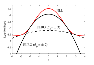
Figure 6.3: Illustration of the ELBO for two different choices of the variational distribution that are tight at different values $\theta_{0}$ of the parameter.

The lower bound property of the ELBO makes it useful not only for the purpose of ML optimization but also as an estimate of LL, and hence of how well the model fits the data, for the goal of model selection. Furthermore, the ELBO can be computed analytically in special cases for exponential models [Wainwright, 2017arXiv171105597Z].

The ELBO can be generalized as the multi-sample ELBO [multisampleELBO]:

$$\ln p(x|\theta)\geq\textrm{E}_{\mathrm{z}_{1},...,\mathrm{z}_{K}\underset{\textrm{i.i.d.}}{\sim}q(z)}\left[\ln\left(\frac{1}{K}\sum_{k=1}^{K}\frac{p(x,\mathrm{z}_{k}|\theta)}{q(\mathrm{z}_{k})}\right)\right].$$ (6.20)

The proof of this inequality follows in the same way as for the ELBO. This bound has the advantage that, as $K$ grows large, it tends to become increasingly accurate. In fact, as $K\rightarrow\infty$, by the law of large numbers, we have the limit $K^{-1}\sum_{k=1}^{K}p(x,\mathrm{z}_{k}|\theta)/q(\mathrm{z}_{k})\rightarrow\sum_{z}p(x,z|\theta)$ with probability one.

ELBO and Bayesian inference. In summary, for a given variational distribution $q(z),$ the ELBO provides an upper bound on the LL function, or equivalently a lower bound on the NLL function. This bound is tight for values of the parameter vectors $\theta$ at which we have the equality $q(z)=p(z|x,\theta)$. As such, given a certain value $\theta$ of the parameter vector, the variational distribution $q(z)$ that provides the tightest bound is the posterior distribution $q(z)=p(z|x,\theta)$, at which the KL divergence in (6.16) vanishes. That is, in order to obtain the tightest ELBO, one needs to solve the Bayesian inference problem of computing the posterior $p(z|x,\theta)$ of the hidden variables for the given value $\theta$. This property can be stated for reference as follows

$$\textrm{arg}\underset{q(z)}{\textrm{max }}\mathcal{L}(q,\theta)=p(z|x,\theta).$$ (6.21)

Gradients of the LL and of the ELBO over the model parameters.^∗ Under suitable differentiability assumptions, the gradient of the ELBO at the value $\theta_{0}$ in which the ELBO is tight coincides with the gradient of the LL, i.e.,

$$\nabla_{\theta}\ln p(x|\theta)|_{\theta=\theta_{0}} =\nabla_{\theta}\mathcal{L}\left(p(z|x,\theta_{0}),\theta\right)|_{\theta=\theta_{0}}$$

$$=\textrm{E}_{\mathrm{z}\sim p(z|x,\theta_{0})}\left[\nabla_{\theta}\ln p(x,\mathrm{z}|\theta)|_{\theta=\theta_{0}}\right].$$ (6.22)

This is also suggested by the curves in Fig. 6.3. We will see with an example in Sec. 6.5.1 that this formula is extremely useful when the gradient for the complete log-likelihood $\nabla_{\theta}\ln p(x,\mathrm{z}|\theta)|_{\theta=\theta_{0}}$ can be easily computed, such as for exponential family models.

Other global lower bounds on the likelihood.^∗ Revisiting the proof of Theorem 6.3.3, it can be concluded that the following general family of lower bounds

$$\text{$f(p(x|$$\theta$)) }\geq\textrm{E}_{z\sim q(z)}\left[f\left(\frac{p(x,z|\theta)}{q(z)}\right)\right],$$ (6.23)

for any concave function $f$. While the ELBO equals the negative of a KL divergence between variational distribution and the true distribution, as seen in (6.13), this representation yields more general divergence measures, such as the $\alpha$-divergence to be discussed in Chapter 8 [LiTurner, 2017arXiv170907433B, 2017arXiv171105597Z].

6.3.3 EM Algorithm

As mentioned, a large number of practical schemes for unsupervised learning using directed and undirected generative models are based on the maximization of ELBO $\mathcal{L}(q,\theta)$ in lieu of the LL function. As seen, this maximization has the key advantage that the ELBO is a concave function of the parameters $\theta$. Furthermore, the lower bound property (6.15) ensures that, if the ELBO is tight at a value $\theta_{0}$, the result of the optimization of the ELBO must necessarily yield a LL value that is no smaller than $\textrm{ln}p(x|\theta_{0})$. This observation is leveraged by the EM algorithm to obtain a procedure that is guaranteed to converge to a stationary point of the original ML problem (6.7).

The EM algorithm is described in Table 6.1.

$\bullet$ Initialize parameter vector $\theta^{\textrm{old}}.$

$\bullet$ E step: For fixed parameter vector $\theta^{\textrm{old}}$, maximize the ELBO over the variational distribution $q$, i.e., solve problem $\underset{q}{\text{max }}\mathcal{L}(q,\theta^{\textrm{old}})$, which, by (6.21), yields the new distribution

$$q^{\textrm{new}}(z)=p(z|x,\theta^{\textrm{old}}).$$ (6.24)

$\bullet$ M step: For fixed variational distribution $q^{\textrm{new}}(z)$, maximize the ELBO over the parameter vector $\theta$, i.e., solve problem $\underset{\theta}{\text{max }}\mathcal{L}(q^{\textrm{new}},\theta)$. This convex problem can be equivalently written as the maximization of the negative energy

$$\underset{\theta}{\text{max }}Q(\theta,\theta^{\textrm{old}})= \textrm{E}_{\mathrm{z}\sim p(z|x,\theta^{\textrm{old}})}\left[\ln p(x,\mathrm{z}|\theta)\right].$$ (6.25)

$\bullet$ If a convergence criterion is not satisfied, set $\theta^{\textrm{new}}\leftarrow\theta^{\textrm{old}}$and return to the E step.

Table 6.1: EM algorithm.

In many problems of interest, the model $p(x,\mathrm{z}|\theta)$ can be taken to be either the product of a prior and a likelihood from the exponential family for directed models, or directly a member of the exponential family for undirected models. In these cases, the problem (6.25) solved in the M step will be seen below via an example to reduce to the corresponding supervised learning problem, with the caveat that the sufficient statistics are averaged over the posterior distribution $p(z|x,\theta^{\textrm{old}})$.

The EM algorithm is an instance of the more general Majorization Minimization (MM) algorithm [MM]. In this class of algorithms, at each iteration, one constructs a tight lower bound of the objective function at the current iterate $\theta^{\textrm{old}}.$ This bound, which should be easy to maximize, is then optimized, yielding the new iterate $\theta^{\textrm{new}}$. The process is illustrated in Fig. 6.4. As it can be seen, at each iteration one is guaranteed that the objective function is not decreased, which ensures convergence to a local optimum of the original problem. In EM, the tight lower bound is the ELBO $\mathcal{L}(q^{\textrm{new}},\theta)$, which is obtained by computing the posterior distribution of the latent variables $q^{\textrm{new}}(z)=p(z|x,\theta^{\textrm{old}})$ at the current iterate $\theta^{\textrm{old}}$.

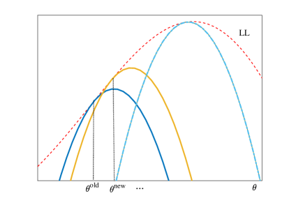
Figure 6.4: Illustration of the EM algorithm. The dashed line is the LL function. The solid lines represent the ELBOs corresponding to the first two steps of the algorithm, while the dashed-dotted line is the ELBO after a number of iterations. At each step, EM maximizes the ELBO, which is a lower bound on the LL function. EM is an instance of the more general MM approach [MM].

Generalizing the $K$-means algorithm, the EM algorithm alternates between: (i) making inferences about the hidden variables $\mathrm{z}$ based on the model defined by the current iterate of the model parameter $\theta$ in the E step; and (ii) updating the model $\theta$ to match the data $x$ and the inferred variables $\mathrm{z}$ in the M step. It is useful to emphasize that unsupervised learning, even in the assumed frequentist approach, entails the Bayesian inference problem of evaluating the posterior of the hidden variables.

Generalization to $N$ observations. We conclude this section by making explicit the generalization of the EM algorithm to the case in which we have $N$ i.i.d. observations. To elaborate, assume that we have pairs of observed/ unobserved i.i.d. variables $(\mathrm{x}_{n},\mathrm{z}_{n})$, whose assumed joint distribution can be written as $p(x^{N},z^{N}|\theta)=\prod_{n=1}^{N}p(x_{n},z_{n}|\theta)$.

E step: The E step requires the computation of the posterior $p(z^{N}|x^{N},\theta)$. This can be seen to factorize across the examples, since we have

$$p(z^{N}|x^{N},\theta)=\frac{p(x^{N},z^{N}|\theta)}{p(x^{N}|\theta)}= \prod_{n=1}^{n}\frac{p(x_{n},z_{n}|\theta)}{p(x_{n}|\theta)}$$

$$= \prod_{n=1}^{n}p(z_{n}|x_{n},\theta)\text{.\text{ }}\text{}$$ (6.26)

Therefore, in order to compute the posterior, we can operate separately for each example in the data set by evaluating $p(z_{n}|x_{n},\theta)$ for all $n=1,...,N$.

M step: In a similar manner, the negative energy function $Q(\theta,\theta^{\textrm{old}})$ to be used in the M step can be computed separately for each example as

$$Q(\theta,\theta^{\textrm{old}}) =\textrm{E}_{\mathrm{z}^{N}\sim p(z^{N}|x^{N},\theta^{\textrm{old}})}\left[\ln p(x^{N},\mathrm{z}^{N}|\theta)\right]$$

$$=\sum_{n=1}^{N}\textrm{E}_{\mathrm{z}_{n}\sim p(z_{n}|x_{n},\theta^{\textrm{old}})}\left[\ln p(x_{n},\mathrm{z}_{n}|\theta)\right],$$ (6.27)

and hence separately for each example. Note that the optimization in the M step should instead be done jointly on (6.27).

Extensions.^∗ The EM algorithm solves the non-convexity problem identified at the beginning of this section by optimizing ELBOs iteratively according to the outlined MM mechanism. Nevertheless, implementing the EM algorithm may be too computationally demanding in practice. In fact, the E step requires to compute the posterior distribution of the latent variables, which may be intractable when the latent space is large; and the M step entails an average over the posterior distribution, which can also be intractable. In Chapter 8, we will see approaches to overcome these problems via approximate inference and learning techniques. For extensions of EM algorithm, we refer to [Barber, pp. 247-248]. In this regard, it is observed here that the EM algorithm applies also to scenarios in which different data points have generally different subsets of unobserved variables.

6.4 Directed Generative Models

In this section, we discuss directed generative models, in which, as seen in Fig. 6.1(a), one posits a parametrized prior $p(z|\theta)$ of the latent variables $\mathrm{z}$ and a parametrized conditional decoding distribution $p(x|z,\theta)$. As discussed, the goal can be that of learning the distribution $p(x)$ of the true data or to extract useful features $\mathrm{z}$. In the latter case, the use of directed generative model is referred to as performing analysis by synthesis. We first discuss two prototypical applications of EM to perform ML learning. We then outline an alternative approach, known as GAN, which can be thought of as a generalization of ML. Accordingly, rather than selecting a priori the KL divergence as a performance metric, as done implicitly by ML, GANs learn at the same time divergence and generative model.

Multi-layer extensions of generative directed models discussed here fall in the category of Helmholtz machines. We refer to, e.g., [dayan1995helmholtz], for a discussion about the task of training these networks via an approximation of the EM algorithm, which uses tools covered in Chapter 8.

6.4.1 Mixture of Gaussians Model

The mixture of Gaussians model can be described by the following directed generative model

$$\mathrm{z}_{n} \sim\textrm{Cat}(\pi)$$ (6.28a)

$$\mathrm{x}_{n}|\mathrm{z} {}_{n}=k\sim\mathcal{N}(\mu_{k},\Sigma_{k}),$$ (6.28b)

with parameter vector $\theta=[\pi$,$\mu_{0},...,\mu_{K-1},\text{$\Sigma$}_{0},...,\Sigma_{K-1}].$ We use one-hot encoding for the categorical variables $z_{n}=[z_{0n},...,z_{(K-1)n}]^{T}.$ Note that this model can be thought as an unsupervised version of the QDA model for the fully observed, or supervised, case studied in Sec. 4.6 (cf. (4.44)). We will see below that the EM algorithm leverages this observation in the M step. Furthermore, it will be observed that EM for mixture of Gaussians generalizes the $K$-means algorithm.

E step. In the E step, as per (6.26), we need to solve the inference problem of computing the posterior $p(z_{kn}|x_{n},\theta^{\textrm{old}})$ for every example $n$ and cluster index $k=0,...,K-1$. In this case, this can be done directly via Bayes’ theorem since the normalization requires to sum only over the $K$ possible values taken by $\mathrm{z}_{n}$, yielding

$$p(z_{kn}=1|x_{n},\theta^{\textrm{old}})=\frac{\pi_{k}^{\textrm{old}}\mathcal{N}(x_{n}|\mu_{k}^{\textrm{old}},\Sigma_{k}^{\textrm{old}})}{\sum_{j=0}^{K-1}\pi_{j}^{\textrm{old}}\mathcal{N}(x_{n}|\mu_{j}^{\textrm{old}},\Sigma_{j}^{\textrm{old}})}\text{\text{.}}$$ (6.29)

M step. In the M step, we need to maximize the negative energy function $Q(\theta,\theta^{\textrm{old}})$ in (6.27). Each term in the sum can be computed directly as

$$\textrm{E}_{\mathrm{z}_{n}\sim p(z_{n}|x_{n},\theta^{\textrm{old}})}\left[\ln p(x_{n},\mathrm{z}_{n}|\theta)\right] =\sum_{k=0}^{K-1}\bar{z}_{kn}\left\{\ln\pi_{k}+\ln\mathcal{N}(x_{n}|\mu_{k},\Sigma_{k})\right\}$$ (6.30)

with

$$\bar{z}_{kn}=\textrm{E}_{\mathrm{z}_{n}\sim p(z_{n}|x_{n},\theta^{\textrm{old}})}\left[\mathrm{z}_{kn}\right]=p(z_{kn}=1|x_{n},\theta^{\textrm{old}}).$$ (6.31)

As it can be easily checked, the function $Q(\theta,\theta^{\textrm{old}})$ equals the LL function of the QDA supervised problem, in which the variables $\mathrm{z}_{n}$ are observed, with the following caveat: the sufficient statistics $z_{kn}$ are replaced by their posterior averages $\bar{z}_{kn}$. As a result, as opposed to supervised learning, EM describes each example $x_{n}$ as being part of all clusters, with the “responsibility” of cluster $k$ being given by $\bar{z}_{kn}$. Having made this observation, we can now easily optimize the $Q(\theta,\theta^{\textrm{old}})$ function by using the ML solutions (4.45) for QDA by substituting $\bar{z}_{kn}$ for the observed variable $t_{kn}$.

Setting $\Sigma_{k}=\epsilon I$ as a known parameter and letting $\epsilon\rightarrow 0$ recovers the $K$-means algorithm [Bishop, p. 443].

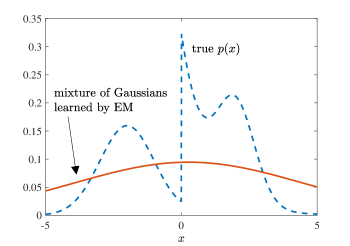
Figure 6.5: True distribution (dashed line) and mixture of Gaussians model learned via EM (solid line).

Example 6.4.1.

Consider data generated from the multi-modal distribution shown in Fig. 6.5 as a dashed line, which obtained as a mixture of two Gaussians and an exponential distribution. When $M=1$, the mixture of Gaussians distribution learned via EM corresponds to the conventional ML estimate, and is hence obtained via moment matching (see Chapter 3). This is plotted in the figure for a given data realization with $N=100$. Running EM with the larger values $M=2$ and $M=3$ also returns the same distribution. This distribution is seen to be inclusive of the entire support of the true distribution and to smooth out the edges of the original distribution. As we will further discuss in Sec. 6.4.3, this is a consequence of the fact that ML minimizes the KL divergence over the second argument.

A similar model that applies to binary data, rather than continuous data, such as black-and-white images, is the mixture of Bernoullis model. The EM algorithm can be derived by following the same steps detailed here [Bishop].

6.4.2 Probabilistic Principal Component Analysis

Probabilistic Principal Component Analysis (PPCA) is a popular generative model that describes the data in terms of $M<D$ features that are linearly related to the data vector. Specifically, PPCA uses a linear factor generative model with $M<D$ features described as

$$\mathrm{z} {}_{n}\sim\mathcal{N}(0,I)$$ (6.32a)

$$\mathrm{x}_{n}|\mathrm{z}_{n} =z\sim\mathcal{N}(Wz+\mu,\sigma^{2}I),$$ (6.32b)

with parameter vector $\theta=(W\textrm{ }\mu\textrm{ }\sigma)$. Equivalently, according to PPCA, the data vector can be written as

$$\mathrm{x}_{n}=W\mathrm{z}_{n}+\mu+\mathrm{q}_{n},$$ (6.33)

with the latent variables $\mathrm{z}{}_{n}\sim\mathcal{N}(0,I)$ and the additive noise $\mathrm{q}_{n}\sim\mathcal{N}(0,\sigma^{2}I)$. According to (6.33), the columns $\{w_{k}\}$ of the matrix $W=[w_{1}\textrm{ }w_{2}\cdots w_{M}]$ can be interpreted as linear features of the data. This is in the sense that each data point is written as a linear combination of the feature vectors as

$$\mathrm{x}_{n}=\sum_{m=1}^{M}w_{m}\mathrm{z}_{mn}+\mu+\mathrm{q}_{n},$$ (6.34)

where $\mathrm{z}_{mn}$ is the $m$th component of the latent vector $\mathrm{z}_{n}$.

In the models studied above, the latent variable was a categorical identifier of the class of the observation. As such, In PPCA, instead, the representation of an observation $x_{n}$ in the hidden variable space is distributed across all the variables in vector $z_{n}$. This yields a more efficient encoding of the hidden representation. This is particularly clear in the case discrete hidden rv, which will be further discussed in Sec. 6.5.1 (see also [bengio2013representation]).

An EM algorithm can be devised to learn the parameter vector as described in [Bishop, p. 577]. The E step leverages the known result that the posterior of the latent variables can be written as

$$\mathrm{z}_{n}|\mathrm{x}_{n}=x_{n},\theta\sim\mathcal{N}(z_{n}|J^{-1}W^{T}(x_{n}-\mu),J^{-1}),$$ (6.35)

with matrix $J=\sigma^{-2}W^{T}W+I$.

We note that, if we model the latent variables $\mathrm{z}_{kn}$, $k=1,...,M$, are independent but not Gaussian, we obtain a type of Independent Component Analysis (ICA) (see [Bishop, p. 591]). It is also possible to impose structure on the latent vector by selecting suitable marginal distributions $p(z)$. For instance, choosing Student’s t-distribution or a Laplace distribution tends to impose sparsity on the learned model. A general discussion on linear factor models can be found in [Murphy] (see also [collins2002generalization] for a generalization of PPCA to any model in the exponential family).

6.4.3 GAN

In Sec. 2.6, we have seen that ML can be interpreted, in the asymptotic regime of a large data set $N$, as minimizing the KL divergence between the true distribution of the data and the model. We start this section by revisiting this argument for unsupervised learning in order to highlight a similar interpretation that holds for finite values of $N$. This viewpoint will lead us to generalize the ML learning approach to techniques in which the choice of the divergence measure is adapted to the data. As an important by-product, the resulting technique, known as GAN, will be seen to accommodate easily likelihood-free models. GANs are currently considered to yield state-of-the-art results for image generation [GoodfellowGANreview].

To simplify the discussion, assume that variables $\mathrm{x}_{n}$ are categorical and take a finite number of values. To start, let us observe that the NLL function (6.1) for i.i.d. data can be written as

$$-\frac{1}{N}\sum_{n=1}^{N}\textrm{ln$p(x_{n}|\theta)=-\sum_{x}\textrm{$\frac{N[x]}{N}$ln$p(x|\theta)$}$,}$$ (6.36)

where we recall that $N[x]=|\{n:\textrm{ $x_{n}=x$}\}|$. We now note that the ML problem of minimizing the NLL (6.36) over $\theta$ is equivalent to the minimization of the KL divergence

$$\underset{\theta}{\min}-\sum_{x}\textrm{$p_{\mathcal{D}}(x)$ln$p(x|\theta)$}+\sum_{x}\textrm{$p_{\mathcal{D}}(x)$ln$p_{\mathcal{D}}(x)$}$$

$$\textrm{=$\underset{\theta}{\min}$ }\textrm{KL}(p_{\mathcal{D}}(x)||p(x|\theta)),$$ (6.37)

where we have defined the empirical distribution

$$p_{\mathcal{D}}(x)=\frac{N[x]}{N}.$$ (6.38)

We hence conclude the ML attempts to minimize the KL divergence between the empirical distribution $p_{\mathcal{D}}(x)$ of the data and the model distribution $p(x|\theta)$. The ML problem min_θ $\textrm{KL}(p_{\mathcal{D}}(x)||p(x|\theta))$ is also known as the M-projection of the data distribution $p_{\mathcal{D}}(x)$ into the model $\{p(x|\theta)\}$ [FnTCsi] (see Chapter 8 for further discussion).

The KL divergence (6.37) is a measure of the difference between two distribution with specific properties that may not be tailored to the particular application of interest. For instance, distributions obtained by minimizing (6.37) tend to provide “blurry” estimates of the distribution of the data distribution, as we have seen in Fig. 6.5. As a result, learning image distributions using M-projections is known to cause the learned model to produce unfocused images [GoodfellowGANreview].

The KL divergence is not, however, the only measure of the difference between two distributions. As discussed in more detail in Appendix A, the KL divergence is in fact part of the larger class of $f$-divergences between two distributions $p(x)$ and $q(x)$. This class includes divergence measures defined by the variational expression

$$D_{f}(p||q)=\max_{T(x)}\textrm{E}_{\mathrm{x}\sim p}[T(\mathrm{x})]-\textrm{E}_{\mathrm{x}\sim q}[g(T(\mathrm{x}))],$$ (6.39)

for some concave increasing function $g(\cdot)$ (the meaning of the $f$ subscript is discussed in Appendix A). The key new element in (6.39) is the decision rule $T(x)$, which is also known as discriminator or critic. This function takes as input a sample $x$ and ideally outputs a large value when $x$ is generated from distribution $p$, and a small value when it is instead generated from $q$. Optimizing over $T(x)$ hence ensures that the right-hand side of (6.39) is large when the two distributions are different and hence can be distinguished based on the observation of $x$. When the domain over which the discriminator $T(x)$ is optimized is left unconstrained, solving problem (6.39) recovers the KL divergence and the Jensen-Shannon divergence, among others, with specific choices of function $g$ (see Appendix A).

Generalizing the ML problem (6.37), GANs attempt to solve the problem

$$\textrm{$\underset{\theta}{\min}$ }D_{f}(p_{\mathcal{D}}(x)||p(x|\theta)).$$ (6.40)

More precisely, GANs parametrize the discriminator $T(x)$ by choosing a differentiable function $T_{\varphi}(x)$ of the parameter vector $\varphi$. This effectively reduces the search space for the discriminator, and defines a different type of divergence for each value of $\varphi$. A typical choice for $T_{\varphi}(x)$ is the output of a multi-layer neural network with weights $\varphi$ or a function thereof (see Sec. 4.5). With this in mind, using (6.39) in (6.40), we obtain the minimax problem solved by GANs

$$\textrm{$\underset{\theta}{\min}$ }\max_{\varphi}\textrm{E}_{\mathrm{x}\sim p_{\mathcal{D}}}[T_{\varphi}(\mathrm{x})]-\textrm{E}_{\mathrm{x}\sim p(x|\theta)}[g(T_{\varphi}(\mathrm{x}))].$$ (6.41)

According to (6.41), GANs select the divergence measure adaptively through the optimization of the discriminator $T_{\varphi}(x)$. Problem (6.41) can also be interpreted in terms of a strategic game played by generator and discriminator [GoodfellowGANreview].

The original GAN method [GoodfellowGANreview] operates by setting $T_{\varphi}(x)=\ln D_{\varphi}(x)$, where $D_{\varphi}(x)$ is the output of a multi-layer perceptron, and $g(t)=-\log(1-\exp(t))$. A variation that is shown to be more useful in practice is also discussed in the first GAN paper (see [Fedus17]). As another popular example, Wasserstein GAN simply sets $T_{\varphi}(x)$ to be the output of a multi-layer perceptron and chooses $g(t)=-(1-t)$.

Application to likelihood-free models.^∗ GANs are typically used with likelihood-free models. Accordingly, the model distribution $p(x|\theta)$ is written as

$$p(x|\theta)=\int\delta(x-G_{\theta}(z))\mathcal{N}(z|0,I)dz.$$ (6.42)

The samples $\mathrm{x}$ are hence modelled as the output of a generator function $G_{\theta}(z)$, whose input $\mathrm{z}$ is given by i.i.d. Gaussian variables. This generative model can hence be interpreted as a generalization of PPCA to non-linear encoders $G_{\theta}(z)$. The latter is conventionally modelled again as a multi-layer neural network.

Problem (6.41) is typically tackled using SGD (Chapter 4) by iterating between the optimization of the generator parameters $\theta$ and of the discriminator parameters $\varphi$ (see [Wasserstein, Algorithm 1]). Learning requires empirical approximations for the evaluation of the gradients that will be discussed in Chapter 8.

Likelihood ratio estimation viewpoint.^∗ When no constraints are imposed over the discriminator $T(x)$ in (6.39) and the function $g$ is selected as $g(t)=\exp(t-1)$, the optimal solution is given as $T(x)=1+\ln(p_{\mathcal{D}}(x)/p(x|\theta))$ and the corresponding divergence measure (6.39) is the KL divergence KL$(p_{\mathcal{D}}(x)||p(x|\theta))$. Therefore, solving problem (6.39) over a sufficiently general family of functions $T_{\varphi}(x)$ allows one to obtain an estimate of the log-likelihood ratio $\ln(p_{\mathcal{D}}(x)/p(x|\theta))$. As a result, GANs can be interpreted as carrying out the estimation of likelihood ratios between the data and the model distributions as a step in the learning process. The idea of estimating likelihood ratios in order to estimate KL divergences is useful in other learning problems based on variational inference, to be discussed in Chapter 8 (see [huszar2017variational]).

Some research topics.^∗ Among topics of current research, we mention here the problem of regularization of GANs [roth2017stabilizing]. We also note that GANs can also be extended to supervised learning problems [odena2016conditional]. The GAN approach of formulating the divergence as an optimization over a discriminator function was also recently found to be useful for ICA [brakel17].

6.5 Undirected Generative Models

Unlike directed generative models, undirected generative models posit a joint distribution for the hidden and the observed variables that captures affinity, rather than causality, relationships between the two sets of variables, as seen in Fig. 6.1(b). In this section, we discuss a representative example of undirected generative models that is considered to be a powerful tool for a number of applications, including feature selection, generation of new samples, and even recommendation systems [RusReccom]. The model, known as RBM, also finds application as a components of larger multi-layer structures, also for supervised learning [Hintoncourse].

6.5.1 Restricted Boltzmann Machines (RBM)

RBMs are typically characterized by an $M$-dimensional binary hidden vector $z\in\{0,1\}^{M}$, while the observed variables may be discrete or continuous. Here we consider the case of binary observed variables, which is suitable to model, e.g., black-and-white images or positive/ negative recommendations. The RBM model is defined as (6.3), where the joint distribution of visible and latent variables is a log-linear model, and hence part of the exponential family. Mathematically, we have

$$p(x,z|\theta)=\frac{1}{Z(\theta)}\exp(-E(x,z|\theta)),$$ (6.43)

with the energy function given as

$$E(x,z|\theta)=-a^{T}z-b^{T}x-x^{T}Wz,$$ (6.44)

and the partition function as $Z(\theta)=\sum_{x,z}\exp(-E(x,z|\theta)).$ The parameter vector $\theta$ includes the $M\times 1$ vector $a$, the $D\times 1$ vector $b$ and the $D\times M$ matrix $W$.

The qualifier “restricted” captures the fact that the energy function (6.44) only features cross-terms that include one variable from $\mathrm{x}$ and one from $\mathrm{z}$, and not two variables from $\mathrm{x}$ or two from $\mathrm{z}$. In other words, the model accounts for the affinities between variables in $\mathrm{x}$ and $\mathrm{z}$, but not directly between variables in either $\mathrm{x}$ or $\mathrm{z}$ [bengio2013representation]. For instance, if ($i,j$)th entry $w_{ij}$ of matrix $W$ is a large positive number, variables $x_{i}$ and $z_{j}$ will tend to have equal signs in order to minimize the energy and hence maximize the probability; and the opposite is true when $w_{ij}$ is negative. As we will seen in the next chapter, this type of probabilistic relationship can be represented by the undirected graphical model known as MRF shown in Fig. 6.6.

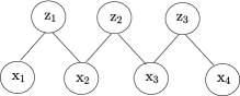
Figure 6.6: An undirected graph (MRF) describing the joint distribution prescribed by the RBM model (6.43)-(6.44).

From the model, it is easy to compute the distribution of each hidden or observed variable when conditioning on all the observed or hidden variables, respectively. In particular, we have that the variables in $\mathrm{z}$ are mutually independent when conditioned on $\mathrm{x}$, and, similarly, the variables in $\mathrm{x}$ are independent given $\mathrm{z}$. Furthermore, the conditional distributions are given as:

$$p(z_{j}=1|x,\theta)= \sigma(w_{j}^{T}x+a_{j})$$ (6.45a)

$$p(x_{i}=1|z,\theta)= \sigma(\tilde{w}_{i}^{T}z+b_{i}),$$ (6.45b)

where $w_{j}$ is the $j$th column of $W$ and $\tilde{w}_{i}$ is the $i$th row of matrix $W$ rearranged into a column vector via transposition. These relationships reveal the significance of the binary hidden variables $z$ in terms of features.

In fact, as for PPCA, we can consider each column of matrix $W$ as a feature vector that contributes in explaining the observations. To see this, note that (6.45a) suggests that the $j$th hidden variable $z_{j}$ equals 1 when the feature $w_{j}$ is well correlated with the data point $x$. Probability (6.45b) also confirms this interpretation, as each variable $z_{j}$ multiplies the $i$th element of the feature vector $w_{j}$ in defining the LLR $\tilde{w}_{i}^{T}z+b_{i}$ (see Sec. 3.2). Furthermore, the distributed representation of the data in terms of the binary hidden vector $z$ is more efficient than that provided by models with categorical variables such as the mixture of Gaussian model. This is in the following sense. While categorical models require to learn a number of parameters that increases linearly with the number of classes, the distributed representation with a binary vector $z$ can distinguish $2^{D}$ combinations of features with a number of parameters that increases only linearly with $D$ [bengio2013representation].

Learning is typically done by means of an approximate SGD method that leverages MC techniques. Recalling the general formula (3.28) for the exponential family, the gradient at the current iteration $\theta=\theta^{\textrm{old}}$ can be computed using (6.22) as

$$\nabla_{w_{ij}}\ln p(x|\theta)|_{\theta=\theta^{\textrm{old}}} =\textrm{E}_{\mathrm{\mathrm{z}}_{j}\sim p(z_{j}|x,\theta^{\textrm{old}})}[x_{i}\mathrm{z}_{j}]-\textrm{E}_{\textrm{$\mathrm{x}_{i},\mathrm{z}_{j}$}\sim p(\textrm{$x,z_{j}$}|\theta^{\textrm{old}})}[\mathrm{x}_{i}\mathrm{z}_{j}],$$ (6.46)

which can be further simplified using (6.45). The gradient presents the structure, noted in Chapter 3, given by the difference between a positive component, which depends on the data $x$, and a negative component, which instead requires an ensemble average over all other possible samples $\textrm{$\mathrm{x}$}\sim p(\textrm{$x$}|\theta^{\textrm{old}})$. Similar relations can be written for the gradients with respect to $a$ and $b$, namely

$$\nabla_{a_{j}}\ln p(x|\theta)|_{\theta=\theta^{\textrm{old}}} =\textrm{E}_{\mathrm{\mathrm{z}}_{j}\sim p(z_{j}|x,\theta^{\textrm{old}})}[\mathrm{z}_{j}]-\textrm{E}_{\mathrm{\mathrm{z}}_{j}\sim p(z_{j}|\theta^{\textrm{old}})}[\mathrm{z}_{j}]$$ (6.47)

and

$$\nabla_{b_{i}}\ln p(x|\theta)|_{\theta=\theta^{\textrm{old}}}=x_{i}-\textrm{E}_{\textrm{$\mathrm{x}_{i}$}\sim p(x_{i}|\theta^{\textrm{old}})}[\mathrm{x}_{i}].$$ (6.48)

In order to evaluate the expectations in the negative components of the gradients, one typically uses a an MC technique known as Markov Chain MC (MCMC) to be discussed in Chapter 8. More specifically, a simplified approach known as Contrastive Divergence (CD) has been found to be an effective approximation. Accordingly, one “clamps” the visible variables to the observed variables $\mathrm{x}=x$, and generates the sequence $x\rightarrow z^{(0)}\rightarrow x^{(1)}\rightarrow z^{(1)}$, using the conditional probability (6.45a) to generate $\mathrm{z}$ from $\mathrm{x}$ and (6.45b) to generate $\mathrm{x}$ from $\mathrm{z}$. The resulting samples are used to approximate the expectations as

$$\nabla_{w_{ij}}\ln p(x|\theta)|_{\theta=\theta^{\textrm{old}}}\simeq x_{i} z_{j}^{(0)}-x_{i}^{(1)}z_{j}^{(1)},$$ (6.49)

and similar expressions apply for the other gradients. The CD scheme can also be generalized to CD-$k$ by increasing the Markov chain sequence to $k$ steps, and the using the resulting samples $x^{(k)}$ and $z^{(k)}$ in lieu of $x^{(1)}$ and $z^{(1)}.$

Extensions and application of the RBM are discussed in [bengio2013representation, welling2005exponential]. Generalizations of RBMs with multiple layers of hidden variables are referred to as Deep Boltzmann Machines. We refer to [Hintoncourse] for discussion about training and applications.

6.6 Discriminative Models

When the goal is learning a representation $\mathrm{z}$ of data $\mathrm{x}$, one can try to directly learn a parametrized encoder, or discriminative model, $p(z|x,\theta)$, as illustrated in Fig. 6.1(c). With an encoder $p(z|x,\theta)$, we can define the joint distribution as $p(x,z|\theta)=p(x)p(z|x,\theta)$, where $p(x)$ is the true distribution of the data. The latter is in practice approximated using the empirical distribution $p_{\mathcal{D}}(x)$ of the data. This yields the joint distribution

$$p(x,z|\theta)=p_{\mathcal{D}}(x)p(z|x,\theta).$$ (6.50)

From (6.50), it is observed that, unlike the frequentist methods considered up to now, discriminative models for unsupervised learning are based on the definition of a single distribution over observed and unobserved variables. As such, divergence measures, which involve two distributions, are not relevant performance metrics. In contrast, a suitable metric is the mutual information between the jointly distributed variables ($\mathrm{x}$,$\mathrm{z}$). The mutual information is a measure of the statistical dependence between the two rvs and is introduced in Appendix A.

To elaborate, a typical learning criterion is the maximization of the mutual information $I_{p(x,z|\theta)}(\mathrm{x};\mathrm{z})$ between the representation $\mathrm{z}$ and the data $\mathrm{x}$ under the joint distribution $p(x,z|\theta)$. Note that, for clarity, we explicitly indicated the joint distribution used to evaluate the mutual information as a subscript. It can be related to the KL divergence as $I_{p(x,z|\theta)}(\mathrm{x};\mathrm{z})=\textrm{KL}(p(x,z|\theta)||p(x)p(z))$. This relationship indicates that the mutual information quantifies the degree of statistical dependence, or the distance from independence, for the two rvs.

The resulting Information Maximization problem is given as

$$\underset{\theta}{\max\textrm{ }}I_{p_{\mathcal{D}}(x)p(z|x,\theta)}(\mathrm{x};\mathrm{z}).$$ (6.51)

As seen, in order to avoid learning the trivial identity mapping, one needs to impose suitable constraints on the encoder $p(z|x,\theta)$ in order to restrict its capacity. In order to tackle problem (6.51), a typical solution is to resort to an MM approach that is akin to the EM algorithm for ML learning described above (see Fig. 6.4).

To this end, as for EM, we introduce a variational distribution $q(x|z)$, and observe that we have the following lower bound on the mutual information

$$I_{p_{\mathcal{D}}(x)p(z|x,\theta)}(\mathrm{x};\mathrm{z})\geq H(p_{\mathcal{D}}(x))+\textrm{E}_{\mathrm{x},\mathrm{z}\sim p_{\mathcal{D}}(x)p(z|x,\theta)}[\ln q(\mathrm{x}|\mathrm{z})].$$ (6.52)

This result follows using the same steps as for the ELBO. The bound is tight when the variational distribution $q(x|z)$ equals the exact posterior $p(x|z,\theta)=p_{\mathcal{D}}(x)p(z|x,\theta)/(\sum_{x}p_{\mathcal{D}}(x)p(z|x,\theta))$. Based on this inequality, one can design an iterative optimization algorithm over the model parameters and the variational distribution $q(x|z)$ (see, e.g., [Akagov05, vincent2010stacked]). When the latter is constrained to lie in a parametrized family, the optimization over the decoder $q(x|z)$ is an example of variational inference, which will be discussed in Chapter 8. The optimization over the model parameters can be simplified when the model has additional structure, such as in the InfoMax ICA method [lee1999independent].

Inference-based interpretation.^∗ The mutual information can be related to the error probability of inferring $\mathrm{x}$ given the representation $\mathrm{z}$. This can be seen, e.g., by using Fano’s inequality [Cover, Akagov05]. More concretely, criterion (6.52) can be interpreted in terms of inference of $\mathrm{x}$ given $\mathrm{z}$ by noting that its right-hand side can be written as the difference $H(p_{\mathcal{D}}(x))-(\textrm{E}_{\mathrm{x},\mathrm{z}\sim p_{\mathcal{D}}(x)p(z|x,\theta)}[-\ln q(\mathrm{x}|\mathrm{z})]).$ In fact, the second term is the cross-entropy measure for the prediction of $\mathrm{x}$ given $\mathrm{z}$ by means of the variational distribution $q(x|z)$. Therefore, by maximizing (6.52) over $\theta$, the model $p(z|x,\theta)$ obtains a representation $z$ such that the predictor $q(x|z)$ ensures, on average, a good reconstruction of $x$ given $z$. This point is further elaborated on in [Alemi17]. We specifically point to [Alemi17, Fig. 2], where a comparison with methods based on ML is provided.

Information bottleneck method.^∗ An important variation of the InfoMax principle yields the information bottleneck method. In the latter, one assumes the presence of an additional variable $\mathrm{y}$, jointly distributed with $\mathrm{x}$, which represents the desired information, but is unobserved. The goal is, as above, to learn an encoder $p(z|x,\theta)$ between the observed $\mathrm{x}$ and the representation $\mathrm{z}$. However, here, this is done by maximizing the mutual information $I(\mathrm{y};\mathrm{z})$ between the target unobserved variable $\mathrm{y}$ and the representation $\mathrm{z}$, in the presence of a regularization term that aims at minimizing the complexity of the representation. This penalty term is given by the mutual information $I(\mathrm{x};\mathrm{z})$, which finds justification in rate-distortion arguments [bottleneck].

6.7 Autoencoders

As seen in Fig. 6.1, autoencoders include parametric models for both encoder and decoder. We focus here for brevity on deterministic autoencoders, in which the encoder is defined by a function $z=F_{\theta}(x)$ and the decoder by a function $x=G_{\theta}(z)$. Note that the parameters defining the two functions may be tied or may instead be distinct, and that the notation is general enough to capture both cases. We will mention at the end of this section probabilistic autoencoders, in which encoder and decoder are defined by conditional probability distributions.

Autoencoders transform the unsupervised learning problem of obtaining a representation $z=F_{\theta}(x)$ of the input $x$ based solely on unlabelled examples $\{x_{n}\}_{n=1}^{N}$ into an instance of supervised learning. They do so by concatenating the encoder $z=F_{\theta}(x)$ with a decoder $x=G_{\theta}(z)$, so as to obtain the input-output relationship $t=G_{\theta}(F_{\theta}(x))$. The key idea is to train this function by setting the target $t$ to be equal to the input $x$. As such, the machine learns to obtain an intermediate representation $z=F_{\theta}(x)$ that makes it possible to recover a suitable estimate $t=G_{\theta}(z)\simeq x$ of $x$.

To formalize the approach, learning is typically formulated in terms of the ERM problem

$$\underset{\theta}{\text{min}}\sum_{n=1}^{N}\ell(x_{n},G_{\theta}(F_{\theta}(x_{n}))),$$ (6.53)

in which, as explained, the encoder-decoder mapping $G_{\theta}(F_{\theta}(\cdot))$ is trained to reproduce the input at its output.

In the absence of constraints on encoder and decoder, the problem above trivially returns an identify mapping, i.e., $G_{\theta}(F_{\theta}(x))=x.$ In order to potentially learn a useful model, one should hence impose constraints, such as dimensionality or sparsity, on the latent vector $z$. Some notable examples are discussed next.

PCA. PCA assumes linear encoder and decoder, and ties their weight matrices via a transposition. Specifically, PCA sets the encoder as $F_{\theta}(x)=W^{T}x$ and the decoder as $G_{\theta}(z)=Wz$. The parameters $\theta$ are hence given by the $D\times M$ matrix $W$. By these definitions, the $M$ columns of $W$ have the interpretation of linear features as for PPCA.

With a quadratic loss function, the learning problem (6.53) is given as

$$\underset{W}{\text{min}}\sum_{n=1}^{N}\|x_{n}-WW^{T}x_{n}\|^{2}.$$ (6.54)

This problem can be solved in closed form. The solution is in fact given by the $M$ principal eigenvectors of the sample covariance matrix $N^{-1}\sum_{n=1}^{N}x_{n}x_{n}^{T}.$ Extensions of PCA that use the kernel trick (Chapter 4) can be also devised (see, e.g., [Murphy]). Furthermore, PCA can be seen to be a special case of PPCA by setting in the latter $\mu=0$ and by taking the limit $\sigma^{2}\rightarrow 0$.

Dictionary learning. In dictionary learning, the decoder is linear, i.e., $G_{\theta}(z)=Wz$, as for PCA. However, the encoder is limited only by constraints on the set of feasible latent variables $z$. A typical such constraint is sparsity: the latent vector should have a small number of non-zero elements. Defining as $\mathcal{C}$ the set of feasible values for $z$, the dictionary learning problem can be formulated as

$$\underset{W,\{z_{n}\}\in\mathcal{C}}{\text{min}}\frac{1}{N}\sum_{n=1}^{N}\|x_{n}-Wz_{n}\|^{2}.$$ (6.55)

The name of the method accounts for the fact that matrix $W$ can be thought of as the dictionary of $M$ features – its columns – that are used to describe the data. The problem above is typically solved using alternate optimization. Accordingly, one optimizes over $W$ for a fixed set of latent vectors $\{z_{n}\}$, which is a standard least squares problem; and the optimizes over each latent vector $z_{n}$ for a fixed $W$. The second problem can be tackled by using standard sparsity-based methods, such as LASSO (Chapter 2).

Multi-layer autoencoders.^∗ One can also represent both encoder and decoder as multi-layer neural networks. In this case, the weights of encoder and decoders are typically tied to be the transpose of one another, in a manner similar to PCA. Training is often done first layer-by-layer, e.g., using RBM training, and then via backpropagation across the entire network [Hintoncourse].

Denoising autoencoders.^∗ An alternative approach to facilitate the learning of useful features is that taken by denoising autoencoders [vincent2010stacked]. Denoising autoencoders add noise to each input $x_{n}$, obtaining a noisy version $\tilde{x}_{n}$, and to then train the machine with the aim of recovering the input $x_{n}$ from its noisy version $\tilde{x}_{n}$. Formally, this can be done by minimizing the empirical risk $\sum_{n=1}^{N}\ell(x_{n},G_{\theta}(F_{\theta}(\tilde{x}_{n})))$.

Probabilistic autoencoders.^∗ Instead of using deterministic encoder and decoder, it is possible to work with probabilistic encoders and decoders, namely $p(z|x,\theta)$ and $p(x|z,\theta)$, respectively. Treating the decoder as a variational distribution, learning can then be done by a variant of the EM algorithm. The resulting algorithm, known as Variational AutoEncoder (VAE), will be mentioned in Chapter 8.

6.8 Ranking^∗

We conclude this chapter by briefly discussing the problem of ranking. When one has available ranked examples, ranking can be formulated as a supervised learning problem [Shalev]. Here, we focus instead on the problem of ranking a set of webpages based only on the knowledge of their underlying graph of mutual hyperlinks. This set-up may be considered as a special instance of unsupervised learning. We specifically describe a representative, popular, scheme known as PageRank [pagerank], which uses solely the web of hyperlinks as a form of supervision signal to guide the ranking.

To elaborate, we define the connectivity graph by including a vertex for each webpage and writing the adjacent matrix as

$$L_{ij}=\begin{cases}1&\text{if page $j$ links to page $i$}\\ 0&\text{otherwise}\end{cases}.$$ (6.56)

The outgoing degree of a webpage is hence given as

$$C_{j}=\sum_{i}L_{ij}.$$ (6.57)

PageRank computes the rank $p_{i}$ of a webpage $i$ as

$$p_{i}=(1-d)+d\sum_{j\neq i}\frac{L_{ij}}{C_{j}}p_{j},$$ (6.58)

where $0<d<1$ is a parameter. Hence, the rank of a page is a weighted sum of a generic rank of equal to 1, which enables the choice of new pages, and of an aggregate “vote” from other pages. The latter term is such that any other page $j$ votes for page $i$ if it links to page $i$ and its vote equals its own rank divided by the total number of outgoing links, that is, $p_{j}/C_{j}$. In essence, a page $i$ is highly ranked if it is linked by pages with high rank. The equation (6.58) can be solved recursively to obtain the ranks of all pages. A variation of PageRank that tailors ranking to an individual’s preferences can be obtained as described in [haveliwala2003topic].

6.9 Summary

In this chapter, we have reviewed the basics of unsupervised learning. A common aspect of all considered approaches is the presence of hidden, or latent, variables that help explain the structure of the data. We have first reviewed ML learning via EM, and variations thereof, for directed and undirected models. We have then introduced the GAN method as a generalization of ML in which the KL divergence is replaced by a divergence measure that is learned from the data. We have then reviewed discriminative models, which may be trained via the InfoMax principle, and autoencoders.

In the next section, we broaden the expressive power of the probabilistic models considered so far by discussing the powerful framework of probabilistic graphical models.

Part IV Advanced Modelling and Inference

Chapter 7 Probabilistic Graphical Models

As we have seen in the previous chapters, probabilistic models are widely used in machine learning. Using Fig. 6.1 as an example, we have encountered both directed and undirected models, which have been used to carry out supervised and unsupervised learning tasks. Graphical models encode structural information about the rvs of interest, both observed and latent. They hence provide a principled way to define parametric probabilistic models with desired features.

The selection of a probabilistic graphical model hence follows the same general rules that have been discussed so far: A more specialized, or structured, model may help reduce overfitting, and hence the generalization gap. This is done, as we will see, by reducing the number of parameters to be learned. On the flip side, specialization may come at the cost of an irrecoverable bias.

In this chapter, we provide an introduction to the vast field probabilistic graphical models, which is a powerful framework that allows us to represent and learn structured probabilistic models. The goal here is to introduce the main concepts and tools, while referring to the extensive treatments in [Koller, Barber, Murphy, Wainwright] for additional information.

7.1 Introduction

In this section, we start by discussing two examples that illustrate the type of structural information that can be encoded by means of probabilistic graphical models. We then provide an overview of this chapter.

As illustrated by the two examples below, structured probabilistic models can be used to set up parametric models for both supervised and unsupervised learning. In the former case, all variables are observed in the training set, with some rvs being inputs, i.e., covariates ($x$), and others being considered as outputs, or targets ($t$). In contrast, in the latter case, some variables are unobserved and play the role of latent variables ($z$) that help explain or generate the observed variables ($x$).

Example 7.1.1.

Consider the tasks of text classification via supervised learning or text clustering via unsupervised learning. In the supervised learning case, the problem is to classify documents depending on their topic, e.g., sport, politics or entertainment, based on set of labelled documents. With unsupervised learning, the problem is to cluster documents according to the similarity of their contents based on the sole observation of the documents themselves.

A minimal model for this problem should include a variable $\mathrm{t}$ representing the topic and a variable $\mathrm{x}$ for the document. The topic can be represented by a categorical variable taking $T$ values, i.e.., $\mathrm{t}\in\left\{1,...,T\right\},$ which is observed for supervised learning and latent for unsupervised learning. As for the document, with “bag-of-words” encoding, a set of $W$ words of interest is selected, and a document is encoded as a $W\times 1$ binary vector $x=[x_{1},...,x_{W}]^{T}$, in which $x_{w}=1$ if word $w$ is contained in the document.

To start, we could try to use an unstructured directed model defined as

$$\mathrm{t\sim}\textrm{Cat}(\pi)$$ (7.1a)

$$\mathrm{x}|\mathrm{t}=t\sim\textrm{Cat}(\pi_{t}),$$ (7.1b)

where the parameter vector includes the $T\times 1$ probability vector $\pi$ and the $T$ probability vectors $\pi_{t},$ one for each class, each of dimension $2^{W}$. Note, in fact, that the vector $\mathrm{x}$ can take $2^{W}$ possible values. As such, this model would require to learn $(T-1)+T(2^{W}-1)$ parameters, which quickly becomes impractical when the number $W$ of words of interest is large enough. Furthermore, as we have seen, a learned model with a large number of parameters is bound to suffer from overfitting if the available data is relatively limited.

Instead of using this unstructured model, we can adopt a model that encodes some additional assumptions that can be reasonably made on the data. Here is one possible such assumption: once the topic is fixed, the presence of a word is independent on the presence of other words. The resulting model is known as Bernoulli naive Bayes, and can be described as follows

$$\mathrm{t}\sim\textrm{Cat}(\pi)$$ (7.2a)

$$\mathrm{x}|\mathrm{t}=t\sim\prod_{w=1}^{W}\textrm{Bern}(x_{w}|\pi_{w|t}),$$ (7.2b)

with parameter vector including the $T\times 1$ probability vector $\pi$ and $T$ sets of $W$ probabilities $\pi_{w|t}$, $w=1,...,W$, for each topic $t$. Parameter $\pi_{w|t}$ represents the probability of word $w$ occurring in a document of topic $t$. The mentioned independence assumption hence allowed us to bring the number of parameters down to $(T-1)+TW$, which corresponds to an exponential reduction.

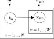
Figure 7.1: BN for the naive Bayes model using the plate notation. Learnable parameters are represented as dots.

The naive Bayes model can be represented graphically by the BN illustrated in Fig. 7.1, where we have considered $N$ i.i.d. documents. Note that the graph is directed: in this problem, it is sensible to model the document as being caused by the topic, entailing a directed causality relationship. Learnable parameters are represented as dots. BNs are covered in Sec. 7.2.

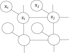
Figure 7.2: MRF for the image denoising example. Only one image is shown and the learnable parameters are not indicated in order to simplify the illustration.

Example 7.1.2.

The second example concerns image denoising using supervised learning. For this task, we wish to learn a joint distribution $p(x,z|\theta)$ of the noisy image $\mathrm{x}$ and of the corresponding desired noiseless image $\mathrm{z}$. We encode the images using a matrix representing the numerical values of the pixels. A structured model in this problem can account for the following reasonable assumptions: (i) neighboring pixels of the noiseless image are correlated, while pixels further apart are not directly dependent on one another; and (ii) noise acts independently on each pixel of the noiseless image to generate the noisy image. These assumptions are encoded by the MRF shown in Fig. 7.2. Note that this is an undirected model. This choice is justified by the need to capture the mutual correlation among neighboring pixels, which cannot be described as a directed causality relationship. We will study MRFs in Sec. 7.3.

As suggested by the examples above, structure in probabilistic models can be conveniently represented in the form of graphs. At a fundamental level, structural properties in a probabilistic model amount to conditional independence assumptions. For instance, in the naive Bayes model, the word indicators are conditionally independent given the topic. As we will see in the rest of this chapter, conditional independence assumptions translate into factorizations of the joint distributions of the variables under study. Factorizations, and associated conditional independence properties, can be represented by three different graphical frameworks, namely BNs, MRFs and factor graphs. For brevity, this chapter will only focus on the first two.

7.2 Bayesian Networks

This section provides a brief introduction to BNs by focusing on key definitions and on the problem of ML learning with some note on MAP and Bayesian viewpoints.

7.2.1 Definitions and Basics

BNs encode a probability factorization or, equivalently, a set of conditional independence relationships through a directed graph. The starting point is the chain rule for probabilities for a generic set of $K$ rvs $\{\mathrm{x}_{1},...,\mathrm{x}_{K}\}$:

$$p(x_{1},...,x_{k}) =p(x_{1})p(x_{2}|x_{1})...p(x_{K}|x_{1},...,x_{K-1}),$$

$$=\prod_{k=1}^{K}p(x_{k}|x_{1},...,x_{k-1}),$$ (7.3)

where the order of the variables is arbitrary. The factorization (7.3) applies for a generic joint distribution, and it does not encode any additional structural information. Note that the notation here is general and not meant to indicate that the variables are necessary observed.

Example 7.2.1.

Consider again the naive Bayes model for text classification/ clustering. There, we imposed the structural constraint that word indicator variables $\{\mathrm{x}_{w}\}_{w=1}^{W}$ be conditionally independent given the topic $\mathrm{t}$. This conditional independence assumption can be expressed using the “perp” notation

$$\mathrm{x}_{w}\perp\{\mathrm{x}_{w^{\prime}}\}_{w^{\prime}\neq w}|\mathrm{t},$$ (7.4)

or the Markov chain notation

$$\mathrm{x}_{w}-\mathrm{t}-\{\mathrm{x}_{w^{\prime}}\}_{w^{\prime}\neq w}.$$ (7.5)

Mathematically, this condition means that we have $p(x_{w}|t,\{x_{w^{\prime}}\})=p(x_{w}|t)$, where $\{x_{w^{\prime}}\}$ is any subset of the variables $\{x_{w^{\prime}}\}_{w^{\prime}\neq w}$. Applying the chain rule to the rvs $(\{\mathrm{x}_{w}\}_{w=1}^{W},\mathrm{t})$ using order $\mathrm{t},\mathrm{x}_{1},...,\mathrm{x}_{W}$ (or any other order on the $\{\mathrm{x}_{w}\}_{w=1}^{W}$ variables), we can hence write

$$p(x,t)=p(t)\prod_{w=1}^{W}p(x_{w}|t).$$ (7.6)

This factorization is represented by the BN in Fig. 7.1. In the directed graph shown in the figure, each vertex corresponds to a rv, and a directed edge is included from $\mathrm{t}$ to each variable $\mathrm{x}_{w}$. This edge captures the fact that the conditional probability of the variable $\mathrm{x}_{w}$ in (7.6) is conditioned on rv $\mathrm{t}$. Informally, $\mathrm{t}$ “causes” all variables in vector $\mathrm{x}.$ The graph accounts for multiple i.i.d. realization $(x_{\mathcal{D}},t_{\mathcal{D}})=\{\mathrm{x}_{n},\mathrm{t}_{n}\}_{n=1}^{N}$, where we denote the $n$th sample as $\mathrm{x}_{n}=[\mathrm{x}_{1n}\cdots\mathrm{x}_{Wn}]^{T}$. The joint distribution factorizes as

$$p(x_{\mathcal{D}},t_{\mathcal{D}})=\prod_{n=1}^{N}p(t_{n})\prod_{w=1}^{W}p(x_{wn}|t_{n}).$$ (7.7)

The BN uses the tile notation that will be formalized below to indicate multiple independent realizations of rvs with the same distribution.

Generalizing the example above, we define BNs as follows.

Definition 7.2.2.

A BN is a directed acyclic graph (DAG), whose vertices represent rvs $\{\mathrm{x}_{1},....,\mathrm{x}_{K}\}$ with an associated joint distribution that factorizes as

$$p(x_{1},...,x_{K})=\underset{k=1}{\prod^{K}}p(x_{k}|x_{\mathcal{P}(k)})$$ (7.8)

where $\mathcal{P}(k)$ denotes the set of parents of node $k$ in the DAG. In a BN, rvs are represented by full circles, while learnable parameters defining the conditional distributions are represented by dots.

As per the definition, the parents $\mathrm{x}_{\mathcal{P}(k)}$ of a rv $\mathrm{x}_{k}$ in the DAG account for the statistical dependence of $\mathrm{x}_{k}$ with all the preceding variables $\mathrm{x}_{1},...,\mathrm{x}_{k-1}$ according to the selected order. That is, the BN encodes the local conditional independence relationships

$$\mathrm{x}_{k}\perp\{\mathrm{x}_{1},...,\mathrm{x}_{k-1}\}|\mathrm{x}_{\mathcal{P}(k)}$$ (7.9)

using the “perp” notation, or equivalently $\mathrm{x}_{k}-\mathrm{x}_{\mathcal{P}(k)}-\{x_{1},...,x_{k-1}\}$ using the Markov chain notation, for $k=1,...,K$. As seen in Fig. 7.1, plates are used to represent independent replicas of a part of the graph.

When to use BNs. BNs are suitable models when one can identify causality relationships among the variables. In such cases, there exists a natural order on the variables, such that rvs that appear later in the order are caused by a subset of the preceding variables. The causing rvs for each rv $\mathrm{x}_{k}$ are included in the parent set $\mathcal{P}(k)$, and are such that, when conditioning on rvs $\mathrm{x}_{\mathcal{P}(k)}$, rv $\mathrm{x}_{k}$ is independent on all other preceding rvs $\{\mathrm{x}_{1},...,\mathrm{x}_{k-1}\}.$ BNs also underlie the framework of interventions that allows the assessment of causality, as opposed to mere correlation, among observed variables, as briefly discussed in Sec. 2.7 [Pearl].

Sampling from a BN. The causality relationship among the ordered variables $\{\mathrm{x}_{1},...,\mathrm{x}_{K}\}$ encoded by a BN makes it easy, at least in principle, to draw samples from a BN. This can be done by using ancestral sampling: Generate rv $\mathrm{x}_{1}\sim$$p(x_{1})$; then, $\mathrm{x}_{2}\sim p(x_{2}|x_{\mathcal{P}(2)})$; and so on, with rv $\mathrm{x}_{k}$ being generated as $\mathrm{x}_{k}\sim p(x_{k}|x_{\mathcal{P}(k)})$.

Example 7.2.3.

Hidden Markov Models (HMMs) are used to study time series, or more generally sequential data, measured through a memoryless transformation, such as an additive noise channel. Mathematically, HMMs can be represented by two sets of variables: the underlying sequence $\mathrm{z}_{1},\mathrm{z}_{2},...,\mathrm{z}_{D},$ and the measured “noisy” data $\mathrm{x}_{1},\mathrm{x}_{2},...,\mathrm{x}_{D}$. HMMs encode two assumptions: (i) each sample $z_{i}$ depends on the past samples only through the previous sample $\mathrm{z}_{i-1}$; and (ii) each measured data $\mathrm{x}_{i}$ depends only on $\mathrm{z}_{i}$. Assumption (i) makes process $\mathrm{z}_{1},\mathrm{z}_{2}$,… a Markov chain.

Using the order $\mathrm{z}_{1},\mathrm{x}_{1},\mathrm{z}_{2},\mathrm{x}_{2},...$, we can write the joint distribution as

$$p(x,z)=p(z_{1})p(x_{1}|z_{1})\prod_{i=1}^{D}p(z_{i}|z_{i-1})p(x_{i}|z_{i})$$ (7.10)

by enforcing the local independencies $\mathrm{z}_{i}-\mathrm{z}_{i-1}-\{\mathrm{z}_{1},...,\mathrm{z}_{i-2},\mathrm{x}_{1},...,\mathrm{x}_{i-2}\}$ and $\mathrm{x}_{i}-\mathrm{z}_{i}-\{\mathrm{z}_{1},...,\mathrm{z}_{i-1},\mathrm{x}_{1},...,\mathrm{x}_{i-1}\}.$ This factorization is represented by the BN in Fig. 7.3. While not indicated in the figure for clarity, an important aspect of HMMs is that the learnable parameters defining the transitions probabilities $p(z_{i}|z_{i-1})$ and the transformations $p(x_{i}|z_{i})$ are respectively imposed to be equal, or tied, for all $i$, hence reducing the number of parameters to be leaned.

Among the many relevant examples of applications of HMMs (see [Koller, Murphy, Barber, rabiner1986introduction]), we mention here text autocorrection, in which the underlying sequential data $\mathrm{z}_{1},\mathrm{z}_{2},...$ amount to the correct text while the measured data $\mathrm{x}_{1},\mathrm{x}_{2},...$ to the typed text; and speech recognition, in which the underlying time series $\mathrm{z}_{1},\mathrm{z}_{2},...$ is a sequence of words and the transformation to the measured recorded speech $\mathrm{x}_{1},\mathrm{x}_{2},...$ translates words into sounds.

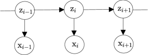
Figure 7.3: BN representing an HMM. The lernable parameters are not explicitly indicated.

In supervised learning applications, both sequences are observed in the training data, with the goal of learning to predict the sequence $\mathrm{z}_{1},\mathrm{z}_{2},...,$ for new measured data points $\mathrm{x}_{1},\mathrm{x}_{2},...$ via to the trained model. This task, in this context, is also known as denoising, since $\mathrm{x}_{1},\mathrm{x}_{2},...$ can be thought of as a noisy version of $\mathrm{z}_{1},\mathrm{z}_{2},...$ With unsupervised learning, only the sequence $\mathrm{x}_{1},\mathrm{x}_{2},...$ is observed.

Example 7.2.4.

This example demonstrates how easily Bayesian modelling can be incorporated in a BN. To this end, consider again the Bernoulli naive Bayes model (7.2) for text classification. Taking a Bayesian viewpoint, parameters $\pi$ and $\{\pi_{w|t}\}$ are to be considered as rvs. We further assume them to be a priori independent, which is known as the global independence assumption. As a result, the joint probability distribution for each document factorizes as

$$p(x,t,\pi,\pi_{w|t}|\alpha,a,b) =\text{Dir}(\pi|\alpha)\textrm{$\prod_{t=1}^{T}\prod_{w=1}^{W}\textrm{Beta}(\pi_{w|t}|a,b)$}$$

$$\times\textrm{Cat}(t|\pi)\prod_{w=1}^{W}\textrm{Bern}(x_{w}|\pi_{w|t}).$$ (7.11)

In the factorization above, we have made the standard assumption of a Dirichlet prior for the probability vector $\pi$ and a Beta prior for parameters $\{\pi_{w|t}\}$, as discussed in Chapter 3. The quantities $\alpha,a,b$ are hyperparameters. Note that the hyperparameters $(a,b)$ are shared for all variables $\pi_{w|t}$ in this example. The corresponding BN is shown in Fig. 7.4, which can be compared to Fig. 7.1 for the corresponding frequentist model.

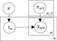
Figure 7.4: BN for the Bayesian version of the naive Bayes model (7.11). Hyperparameters are not indicated and tiles indices are marked without their ranges for clarity.

We invite the reader to consider also the Latent Dirichlet Allocation (LDA) model and the other examples available in the mentioned textbooks.

7.2.2 Global Conditional Independence

As we have discussed, BNs are defined by local conditional independence properties that are encoded in the factorization of a joint distribution and in the supporting DAG. BNs can also be used to assess generic global conditional independence queries of the type: Is a given subset of variables $\mathcal{A}$ independent of another set $\mathcal{B}$ conditioned on a third subset $\mathcal{C}$ of variables? The $d$-separation algorithm outputs either a positive response or a “maybe” answer to this question. It is briefly described as follows:

$\bullet$ Build a subgraph $\mathcal{G}^{\prime}$ from the original DAG by keeping all vertices in the subsets $\mathcal{A}$, $B$ and $\mathcal{C}$, as well as all the edges and vertices encountered by moving backwards on the DAG one or more edges from the vertices in $\mathcal{A}$, $B$ and $\mathcal{C}$;

$\bullet$ Build a subgraph $\mathcal{G}^{\prime\prime}$ from $\mathcal{G}^{\prime}$ by deleting all edges coming out of the vertices in $\mathcal{C}$;

$\bullet$ If there no path, neglecting the directionality of the edges, between a node in $\mathcal{A}$ and a node in $\mathcal{B}$, then the conditional independence relation $\mathcal{A}\perp\mathcal{B}|\mathcal{C}$ holds. Else, if one such path exists, then there is at least one joint distribution that factorizes as for the given DAG for which the condition $\mathcal{A}\perp\mathcal{B}|\mathcal{C}$ does not hold.

Example 7.2.5.

Consider the so-called V-structure $\mathrm{x}\rightarrow\mathrm{y}\leftarrow\mathrm{z}$. Using $d$-separation, it can be seen that the conditional independence $x-y-z$ does not hold in general.

7.2.3 Learning

Assume that the DAG of a BN is given. Structure learning, that is, the decision of which edges should be included in the graph based on available training data, is also an important problem that will not be considered here. Making explicit the dependence of the probability factors on learnable parameters $\mu$, the joint distribution encoded by a BN can be written as

$$p(x_{1},...,x_{K})=\underset{k=1}{\prod^{K}}p(x_{k}|x_{\mathcal{P}(k)},\mu_{k|x_{\mathcal{\mathcal{P}}(k)}}),$$ (7.12)

where $\mu_{k|x_{\mathcal{\mathcal{P}}(k)}}$ are the parameters defining the conditional distribution $p(x_{k}|x_{\mathcal{P}(k)})$. Note that the parameters $\mu_{k|x_{\mathcal{\mathcal{P}}(k)}}$ are generally different for different values of $k$ and of the parents’ variables $x_{\mathcal{\mathcal{P}}(k)}$ (see, e.g., (7.11)). In most cases of interest, the probability distribution $p(x_{k}|x_{\mathcal{P}(k)},\mu_{k|x_{\mathcal{P}(k)}})$ is in the exponential family or is a GLM (see Chapter 3).

As we have already seen in previous examples, the parameters $\mu_{k|x_{\mathcal{P}(k)}}$ can either be separate, that is, distinct for each $k$ and each value of $x_{\mathcal{P}(k)}$, or they can be tied. In the latter case, some of the parameters $\mu_{k|x_{\mathcal{P}(k)}}$ are constrained to be equal across different values of $x_{\mathcal{P}(k)}$ and/or across different values of $k$. As a special case of tied parameters, the value of $\mu_{k|x_{\mathcal{P}(k)}}$ may also be independent of $x_{\mathcal{P}(k)}$, such as in the case for GLMs.

As for the data, we have seen that the rvs $\mathrm{x}_{1},...,\mathrm{x}_{K}$ can be either fully observed in the training set, as in supervised learning, or they can be partially observed as in unsupervised learning.

For the sake of brevity, here we describe learning only for the case of fully observed data with separate parameters, and we briefly mention extensions to the other cases.

Fully Observed Data with Separate Parameters

We are given a fully observed data set $\mathcal{D}=\{x_{n}\}_{n=1}^{N}$, with each data point written as $x_{n}=[x_{1n},...,x_{Kn}]^{T}$. For concreteness, assume that all variables are categorical. Denoting as $\mathrm{x}_{\mathcal{P}(k)n}$ the parents of variable $\mathrm{x}_{kn}$, the LL function can be factorized as:

$$\ln p(\mathcal{D}|\mu) =\sum_{n=1}^{N}\sum_{k=1}^{K}\ln p(x_{kn}|x_{\mathcal{P}(k)n},\mu_{k|x_{\mathcal{P}(k)n}})$$ (7.13a)

$$=\sum_{k=1}^{K}\sum_{n=1}^{N}\ln p(x_{kn}|x_{\mathcal{P}(k)n},\mu_{k|x_{\mathcal{P}(k)n}})$$ (7.13b)

$$=\sum_{k=1}^{K}\sum_{x_{\mathcal{P}(k)}}\sum_{n\in\mathcal{N}_{x_{\mathcal{P}(k)}}\textrm{ }}\ln p(x_{kn}|x_{\mathcal{P}(k)},\mu_{k|x_{\mathcal{P}(k)}}),$$ (7.13c)

where we have defined the set of indices

$$\mathcal{N}_{x_{\mathcal{P}(k)}}=\{n:\textrm{ }x_{\mathcal{P}(k)n}=x_{\mathcal{P}(k)}\}.$$ (7.14)

This set includes the indices $n$ for which the parents $\mathrm{x}_{\mathcal{P}(k)n}$ of node $k$ take a specific vector of values $x_{\mathcal{P}(k)}$. In (7.13c), the inner sum depends only on the parameters $\mu_{k|x_{\mathcal{P}(k)}}$corresponding to the given value $x_{\mathcal{P}(k)}$ of the rvs $\mathrm{x}_{\mathcal{P}(k)n}$ for $n=1,...,N$. Therefore, in the case of separate parameters, the ML estimate for each parameter $\mu_{k|x_{\mathcal{P}(k)}}$ can be carried out independently. While this simplifies the problem, it may also cause overfitting issues owing to the problem of data fragmentation, as each parameter is estimated based only on a fraction of the data set.

As an even more concrete example, consider binary variables modelled as $\mathrm{x}_{k}\sim\textrm{Bern}$$(\mu_{k|x_{\mathcal{P}(k)}}).$ Accordingly, the probability of each rv depends on the value $x_{\mathcal{P}(k)}$ of the parents. For this case, we can write the ML estimate as

$$\hat{\mu}_{k|x_{\mathcal{P}(k)},ML}=\frac{\sum_{n\in\mathcal{N}_{x_{\mathcal{P}(k)}}}x_{kn}}{\left|\mathcal{N}_{x_{\mathcal{P}(k)}}\right|}.$$ (7.15)

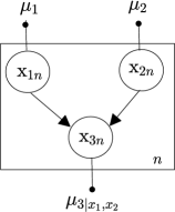
Figure 7.5: BN for Example 7.2.6.

Example 7.2.6.

Consider the BN shown in Fig. 7.5 with binary rvs in the alphabet $\{0,1\}$. The observed data $\mathcal{D}$ is given as

$$\left\{\underset{10}{\underbrace{\left(\begin{array}[]{c}1\\ 0\\ 1\end{array}\right)}},\underset{14}{\underbrace{\left(\begin{array}[]{c}0\\ 1\\ 1\end{array}\right)}},\underset{8}{\underbrace{\left(\begin{array}[]{c}1\\ 1\\ 0\end{array}\right)}},\underset{12}{\underbrace{\left(\begin{array}[]{c}0\\ 0\\ 0\end{array}\right)}},\underset{1}{\underbrace{\left(\begin{array}[]{c}1\\ 0\\ 0\end{array}\right)}},\underset{2}{\underbrace{\left(\begin{array}[]{c}0\\ 1\\ 0\end{array}\right)}},\underset{1}{\underbrace{\left(\begin{array}[]{c}1\\ 1\\ 1\end{array}\right)}},\underset{2}{\underbrace{\left(\begin{array}[]{c}0\\ 0\\ 1\end{array}\right)}}\right\},$$

where the bottom row indicates the number of observations equal to the vector above it. The ML estimates are: $\mu_{1,ML}=\frac{10+8+1+1}{50}=\frac{20}{50}=\frac{2}{5}$, $\mu_{2,ML}=\frac{14+8+2+1}{50}=\frac{1}{2}$, $\hat{\mu}_{3|00}=\frac{2}{12+2}=\frac{1}{7},$ $\hat{\mu}_{3|11}=\frac{1}{8+1}=\frac{1}{9}$, $\hat{\mu}_{3|01}=\frac{14}{14+2}=\frac{7}{8}$ and $\hat{\mu}_{3|10}=\frac{10}{10+1}=\frac{10}{11}$.

MAP estimates can be seen to decompose in a similar way under global independence assumptions on the parameters, and the same holds for Bayesian approach [Koller].

Notes on the General Case

With shared parameters, obtaining ML and MAP estimates require aggregating statistics across all variables that share the same parameters. The Bayesian approach is more complex, and we refer to [Koller] for discussion. An alternative approach with “soft sharing” is the hierarchical Bayes model (see [Koller, Fig. 17.11]). In the presence of missing data, learning typically involves the EM algorithm described in Chapter 6 or approximate learning counterparts to be introduced in the next chapter.

7.3 Markov Random Fields

In this section, we turn to MRF by following the same approach as for BNs in the previous section.

7.3.1 Definitions and Basics

As BNs, MRFs encode a probability factorization or, equivalently, a set of conditional independence relationships. They do so, however, through an undirected graph.

Definition 7.3.1.

A MRF is an undirected graph, whose vertices represent rvs with associated joint distribution that factorizes as

$$p(x)=\frac{1}{Z}\underset{c}{\prod}\psi_{c}(x_{c}),$$ (7.16)

where $c$ is the index of a clique in the graph; $\mathrm{x}_{c}$ is the set of rvs associated with the vertices in clique $c$; $\psi_{c}(x_{c})\geq 0$ is the factor or potential for clique $c$; and $Z=\underset{x}{\sum}\underset{c}{\prod}\psi_{c}(x_{c})$ is the partition function. With no loss of generality, the sum can be limited to maximal cliques (i.e., cliques that are not fully included in a larger clique). In a MRF, rvs are represented by full circles, while learnable parameters defining the conditional distributions are represented by dots.

Each factor $\psi_{c}(x_{c})$ in (7.16) encodes the compatibility of the values $x_{c}$ in each clique, with larger values of $\psi_{c}(x_{c})$ corresponding to configurations $x_{c}$ that are more likely to occur. Factors are generally not probability distributions, i.e., they are not normalized to sum or integrate to one. Furthermore, unlike BNs, each factor does not distinguish between conditioning and conditioned rvs. Rather, all variables in the clique $x_{c}$ can play the same role in defining the value of the potential $\psi_{c}(x_{c})$.

When to use MRFs. This discussion points to the fact that MRFs are especially well suited to model mutual relationships of compatibility, or lack thereof, among variables, rather than causality effects.

Evaluating Probabilities and Sampling from an MRF. This distinguishing feature of MRF, which brings potential modelling advantages in some applications, comes with the added difficulty of evaluating the joint probability distribution and sampling from the joint distribution. In fact, the computation of the probability (7.16) requires the calculation of the partition function $Z$, which is generally intractable when the alphabet of the vector $\mathrm{x}$ is large enough. This is typically not the case for BNs, in which each conditional probability is conventionally selected from a known (normalized) distribution. Furthermore, unlike BNs, MRFs do not allow ancestral sampling, as all the conditional distributions of the individual rvs in $\mathrm{x}$ are generally tied together via the partition function.

Example 7.3.2.

The image denoising example described at the beginning of this chapter leverages the MRF in Fig. 7.2. In it, the maximal cliques are given by the pairs of rvs {$\mathrm{z}_{i},\mathrm{z}_{j}$} and $\{\mathrm{x}_{i},\mathrm{z}_{i}\}$ that are connected by an edge. Associating a factor or potential to each clique yields the factorized joint distribution

$$p(x,z)=\frac{1}{Z}\underset{\{i,j\}}{\prod}\psi_{i,j}(z_{i},z_{j})\cdot\underset{i}{\prod}\psi_{i}(z_{i},x_{i}),$$ (7.17)

where $\{i,j\}$ represents an edge of the undirected graph. As a notable example, in the Ising model, the variables are bipolar, i.e., $\mathrm{z}_{i},\mathrm{x}_{i}\in\{-1,+1$}, and the potentials are defined as $\psi_{ij}(z_{i},z_{j}|\eta_{1})=\textrm{exp}(-E(z_{i},z_{j}|\eta_{1}))$ and $\psi_{i}(z_{i},x_{i}|\eta_{2})=\textrm{exp}(-E(z_{i},x_{i}|\eta_{2}))$, with energy functions

$$E(z_{i},z_{j}|\eta_{1})=-\eta_{1}z_{i}z_{j}\textrm{ and }E(z_{i},x_{i}|\eta)=-\eta_{2}z_{i}x_{i}.$$ (7.18)

From this definition, a large natural parameter $\eta_{1}>0$ yields a large probability – or a low energy – when $z_{i}$ and $z_{j}$ are equal; and, similarly, a large $\eta_{2}>0$ favors configurations in which $z_{i}=x_{i}$, that is, with low noise.

Example 7.3.3.

Another related example is given by the RBMs studied in Sec. 6.5.1, whose undirected graph is shown in Fig. 6.6.

As illustrated by the previous examples, potentials are typically parameterized using the energy-based form

$$\psi_{c}(x_{c})=\textrm{exp}(-E_{c}(x_{c}|\eta_{c})),$$ (7.19)

with parameter vector $\eta_{c}.$ This form ensures that the factors are strictly positive as long as the energy is upper bounded. A special class of such models is given by log-linear models, such as the Ising model, in which, as seen in Chapter 3, the energy is a linear function of the parameters.

7.3.2 Global Conditional Independence

MRF, in a manner similar to BNs, enable the assessment of conditional independence properties globally in the graph. The procedure is, in fact, easier with MRFs thanks to the Hammersley–Clifford theorem. The latter says that, if the potentials $\psi_{c}(x_{c})$ are strictly positive for all cliques $c$, as for the energy-based potentials (7.19), the conditional independence relationship $\mathcal{A}\perp\mathcal{B}|\mathcal{C}$ can be tested via the following simple algorithm.

$\bullet$ Eliminate all variables in $\mathcal{C}$ and all the connected edges;

$\bullet$ If there is no path between rvs in $\mathcal{A}$ and $\mathcal{B}$, then the relationship $\mathcal{A}\perp\mathcal{B}|\mathcal{C}$ holds; if, instead, there is a path, then there exists at least one joint distribution that factorizes as for the undirected graph at hand for which the relationship $\mathcal{A}\perp\mathcal{B}|\mathcal{C}$ does not hold.

7.3.3 Learning

Learning in MRFs is made complicated by the partition function. In fact, the partition function couples together all the parameters. This makes it impossible to carry out separately the estimate of the parameters $\eta_{c}$ associated with each clique even in the fully observed case with separate parameters. Nevertheless, MRFs with energy-based potentials (7.19) fall either in the exponential family, when the factors are log-normal, or in the more general class of energy-based models. In both cases, gradient-based algorithms can be devised by using methods similar to those used in Sec. 6.5.1 for RBMs.

7.3.4 Converting BNs to MRFs

As suggested by the discussion above, BNs and MRFs are suitable to encode different types of statistical dependencies, with the former capturing causality while the latter accounting for mutual compatibility. There are in fact conditional independence properties that can be expressed by BN or MRF but not by both. An example is the V-structure $\mathrm{x}\rightarrow\mathrm{y}\leftarrow\mathrm{z}$ discussed in Example 7.2.5, whose independencies cannot be captured by an MRF.

That said, given a BN with factorization (7.8), we can define potential functions

$$\psi_{k}(x_{k},x_{\mathcal{P}(k)})=p(x_{k}|x_{\mathcal{P}(k)})$$ (7.20)

to obtain the factorization

$$p(x)=\underset{k=1}{\prod^{K}}\psi_{k}(x_{k},x_{\mathcal{P}(k)})$$ (7.21)

with partition function $Z=1$. This factorization defines an MRF in which each maximal clique contains a rv $\mathrm{x}_{k}$ and its parents $\mathrm{x}_{\mathcal{P}(k)}$. The corresponding undirected graph can be directly obtained from the DAG that defines the BN via the following two steps:

$\bullet$ Connect all pairs of parents by an undirected edge – this step is known as “moralization”;

$\bullet$ Make all edges undirected.

As per the discussion above, the resulting MRF may not account for all the independencies encoded in the original graph. This can be easily seen by applying the procedure to the V-structure.

7.4 Bayesian Inference in Probabilistic Graphical Models

Bayesian inference amounts to the computation of the posterior probability of unobserved, or latent, variables given observed variables. In this regard, it is useful to differentiate between intensive and extensive latent variables. Intensive latent variables are model parameters whose number does not increase with the number $N$ of data points, such as the probability vectors $(\pi$,$\{\pi_{w|t}\})$ in the Bernoulli naive Bayes model. Extensive latent variables are instead rvs indexed by the example index $n$, whose number grows with the sample size $N$. These correspond to the latent variables $\mathrm{z}_{n}$ introduced in the previous chapter.

Bayesian inference is a fundamental task that lies at the heart of both inference and learning problems. As seen in Chapter 2, it underlies supervised learning for generative probabilistic models, which requires the computation of the predictive probability $p(t|x,\theta)$ for the new sample ($\mathrm{x}$,$\mathrm{t}$) from the learned model $p(x,t\text{|}\theta)$. It is also at the core of Bayesian supervised learning, which evaluates the posterior $p(\theta|\mathcal{D})$ of the parameter vector $\theta$ (an intensive variable) in order to obtain the predictive posterior $p(t|x,\mathcal{D})=\int p(\theta|\mathcal{D})p(t|x,\theta)d\theta$ for the new sample ($\mathrm{x},\mathrm{t}$). As studied in Chapter 6, Bayesian inference is a key step in unsupervised learning even under a frequentist viewpoint, since the EM algorithm requires the evaluation of the posterior $p(z_{n}|x_{n},\theta$) of the latent (extensive) variables $\{z_{n}\}$ given the current iterate $\theta.$

As discussed, when performing Bayesian inference, we can distinguish between observed variables, say $\mathrm{x}$, and latent variables $\mathrm{z}$. In general, only a subset of latent variables may be of interest, say $\mathrm{z}_{i}$, with the rest of the rvs in $\mathrm{z}$ being denoted as $\mathrm{z}_{-i}.$ The quantity to be computed is the posterior distribution

$$p(z_{i}|x)=\frac{p(x,z_{i})}{p(x)},$$ (7.22)

where

$$p(x,z_{i}) =\sum_{z_{-i}}p(x,z)$$ (7.23)

and

$$\textrm{ $p(x)=\sum_{z_{i}}p(x,z_{i})$},$$ (7.24)

with the sum being replaced by an integral for continuous variables. The key complication in evaluating these expressions is the need to sum over potentially large sets, namely the domains of variables $\mathrm{z}_{-i}$ and $\mathrm{z}_{i}$. Note that the sum in (7.23), which appears at the numerator of (7.22), is over all hidden variables that are of no interest. In contrast, the sum in (7.24), which is at the denominator of (7.22), is over the variables whose posterior probability (7.22) is the final objective of the calculation.

The complexity of the steps (7.23) and (7.24) is exponential in the respective numbers of latent variables over which the sums are computed, and hence it can be prohibitive.

Example 7.4.1.

Consider an HMM, whose BN is shown in Fig. 7.3. Having learned the probabilistic model, a typical problem is that of inferring a given hidden variable $\mathrm{z}_{i}$ given the observed variables $\mathrm{x=\{x}_{1},....,\mathrm{x}_{D}\}$. Computing the posterior $p(z_{i}|x)$ requires the evaluation of the sums in (7.23) and (7.24). When the hidden variables $\mathrm{z}_{1},...,\mathrm{z}_{D}$ are discrete with alphabet size $\mathcal{Z}$, the complexity of step (7.23) is of the order $\left|\mathcal{Z}\right|{}^{D-1}$, since one needs to sum over the $\left|\mathcal{Z}\right|{}^{D-1}$ possible values of the hidden variables.

The structure encoded by probabilistic graphic models can help reduce the discussed complexity of Bayesian inference. Therefore, probabilistic graphical models can not only enhance learning by controlling the capacity of the model, but also enable Bayesian inference. To elaborate, consider a joint distributions defined by an MRF as in (7.16). Note that, as we have seen in Sec. 7.3.4, one can easily convert BNs into MRFs, although possibly at the cost of not preserving some linear independence relationship. With this factorization, the marginalizations (7.23)-(7.24) require solving the so-called sum-product inference task

$$\underset{z}{\sum}\underset{c}{\prod}\psi_{c}(x_{c}),$$ (7.25)

where the variables $\mathrm{z}$ are a subset of the variables in x.

As an important observation, formulation (7.25) highlights the fact that the problem of computing the partition function $Z$ for MRFs is a special case of the sum-product inference task. In fact, in order to compute $Z$, the sum in (7.25) is carried out over all variables in $\mathrm{x}$.

When the undirected graph describing the joint distribution is a tree, the complexity of sum-product inference becomes exponential only in the maximum number of variables in each factor, also known as treewidth of the graph. In this case, the sum-product inference problem can be exactly solved via message passing belief propagation over the factor graph associated to the MRF. We refer to the textbooks [Koller, Barber, Murphy] for details on factor graphs and belief propagation.

Example 7.4.2.

The MRF associated with an HMM is obtained from the BN in Fig. 7.3 by simply substituting directed for undirected edges, and the distribution (7.10) factorizes as

$$p(x,z)=\psi(z_{1})\psi(x_{1},z_{1})\prod_{i=1}^{D}\psi(z_{i},z_{i-1})\psi(x_{i},z_{i}).$$ (7.26)

The undirected graph is a tree with treewidth equal to 2, since, as per (7.26), there are at most two variables in each clique. Therefore, belief propagation allows to evaluate the posteriors $p(z_{i}|x)$ with a complexity of the order $\left|\mathcal{Z}\right|{}^{2}$, which does not scale exponentially with the number $D$ of time samples.

When the undirected graph is not a tree, one can use the junction tree algorithm for exact Bayesian inference. The idea is to group subsets of variables together in cliques, in such a way that the resulting graph is a tree. The complexity depends on the treewidth of the resulting graph. When this complexity is too high for the given application, approximate inference methods are necessary. This is the subject of the next chapter.

7.5 Summary

Probabilistic graphical models encode a priori information about the structure of the data in the form of causality relationships – via directed graphs and BNs – or mutual affinities – via undirected graphs and MRFs. This structure translates into conditional independence conditions. The structural properties encoded by probabilistic graphical models have the potential advantage of controlling the capacity of a model, hence contributing to the reduction of overfitting at the expense of possible bias effects (see Chapter 5). They also facilitate Bayesian inference (Chapters 2-4), at least in graphs with tree-like structures. Probabilistic graphical models can be used as the underlying probabilistic framework for supervised, unsupervised, and semi-supervised learning problems, depending on which subsets of rvs are observed or latent.

While graphical models can reduce the complexity of Bayesian inference, this generally remains computationally infeasible for most models of interest. To address this problem, the next chapter discusses approximate Bayesian inference, as well as associated learning problems (Chapter 6).

Chapter 8 Approximate Inference and Learning

In Chapters 6 and 7, we have seen that learning and inference tasks are often made difficult by the need to compute the posterior distribution $p(z|x)$ of an unobserved variables $\mathrm{z}$ given an observed variables $\mathrm{x}$. This task requires the computation of the normalizing marginal

$$p(x)=\sum_{z}p(x,z),$$ (8.1)

where the sum is replaced by an integral for continuous variables. This computation is intractable when the alphabet of the hidden variable $z$ is large enough. Chapter 7 has shown that the complexity of computing (8.1) can be alleviated in the special case in which the factorized joint distribution $p(x,z)$ is defined by specific classes of probabilistic graphical models.

What to do when the complexity of computing (8.1) is excessive? In this chapter, we provide a brief introduction to two popular approximate inference approaches, namely MC methods and Variational Inference (VI). We also discuss their application to learning. As for the previous chapter, the reader is referred to [Koller, Barber, Murphy, Wainwright] for details and generalizations (see also [Schniterreview]).

8.1 Monte Carlo Methods

To introduce MC methods, we start by observing that the expression (8.1) can be rewritten as the ensemble average

$$p(x)=\sum_{z}p(z)p(x|z)=\textrm{E}_{\mathrm{z}\sim p(z)}[p(x|\mathrm{z})]$$ (8.2)

over the latent rvs $\mathrm{z}\text{$\sim$$p(z)$}$. The general idea behind MC methods is replacing ensemble averages with empirical averages over randomly generated samples. In the most basic incarnation of MC, $M$ i.i.d. samples $\mathrm{z}_{m}\sim p(z)$, $m=1,...,M,$ are generated from the marginal distribution $p(z)$ of the latent variables, and then the ensemble average (8.2) is approximated by the empirical average

$$p(x)\simeq\frac{1}{M}\sum_{m=1}^{M}p(x|\mathrm{z}_{m}).$$ (8.3)

By the law of large numbers, we know that this estimate is consistent, in the sense that it tends with probability one to the ensemble average (8.2) when $M$ is large. Furthermore, the error of the approximation scales as $1/\sqrt{M}$.

Example 8.1.1.

Consider the Ising model for image denoising introduced in Example 7.3.2. We recall that the joint distribution can be factorized as

$$p(x,z)=\frac{1}{Z}\underset{\{i,j\}}{\prod}\psi_{i,j}(z_{i},z_{j})\cdot\underset{i}{\prod}\psi_{i}(z_{i},x_{i}),$$ (8.4)

where $\{i,j\}$ represents an edge of the undirected graph, with energy-based potentials $\psi_{ij}(z_{i},z_{j})=\textrm{exp}(\eta_{1}z_{i}z_{j})$ and $\psi_{i}(z_{i},x_{i})=\textrm{exp}(\eta_{2}z_{i}x_{i}).$ We have removed the dependence of the potentials on the (natural) parameters $\eta_{1}$ and $\eta_{2}$ for simplicity of notation. In order to compute the posterior $p(z|x),$ which may be used for image denoising, the MC approach (8.3) requires to sample from the marginal $p(z)$. This is, however, not easy given the impossibility to perform ancestral sampling over MRFs as discussed in Sec. 7.3.

Importance Sampling. As seen in the previous example, the MC procedure explained above is not always feasible in practice, since drawing samples from the marginal $p(z)$ may not be tractable. For instance, the marginal $p(z)$ may not be known or it may be difficult to draw samples from it. In such common cases, one can instead resort to a simplified distribution $q(z)$ from which sampling is easy. This distribution typically has convenient factorization properties that enable ancestral sampling.

The starting observation is that the marginal distribution (8.1) can be expressed as an ensemble average over a rv $\mathrm{z}\sim q(z)$ as

$$p(x) =\sum_{z}p(z)p(x|z)\frac{q(z)}{q(z)}$$ (8.5)

$$=\sum_{z}q(z)\frac{p(z)}{q(z)}p(x|z)$$

$$=\textrm{E}_{\mathrm{z}\sim q(z)}\left[\frac{p(\mathrm{z})}{q(\mathrm{z})}p(x|\mathrm{z})\right],$$

as long as the support of distribution $q(z)$ contains that of $p(z)$. This expression suggests the following empirical estimate, which goes by the name of Importance Sampling: Generate $M$ i.i.d. samples $\mathrm{z}_{m}\sim q(z)$, $m=1,...,M,$ and then compute the empirical approximation

$$p(x)\simeq\frac{1}{M}\sum_{m=1}^{M}\frac{p(\mathrm{z}_{m})}{q(\mathrm{z}_{m})}p(x|\mathrm{z}_{m}).$$ (8.6)

This estimate is again consistent, but its variance depends on how well $q(z)$ approximates $p(z)$. Note this approach requires knowledge of the marginal $p(z)$ but not the ability to sample from it.

Markov Chain Monte Carlo (MCMC) via Gibbs Sampling. Rather than drawing samples from a distribution that mimics $p(z)$ in order to compute an approximation of the posterior $p(z|x)=p(x,z)/p(x)$, MCMC methods aim at obtaining samples $\{\mathrm{z}_{m}$} directly from the posterior $p(z|x)$. With such samples, one can compute empirical approximations of any ensemble average with respect to $p(z|x)$. This is sufficient to carry out most tasks of interest, including the expectation needed to evaluate the predictive posterior in Bayesian methods for supervised learning or the average energy in the EM algorithm.

MCMC methods generate a sequence of correlated samples $\mathrm{z}_{1},\mathrm{z}_{2},...$ from an easy-to-sample Markov chain $\mathrm{z}_{1}-\mathrm{z}_{2}-...$ that has the key property of having the desired distribution $p(z|x)$ as the stationary distribution. Such a Markov chain can be designed automatically once a BN or MRF factorization of the joint distribution is available. To this end, Gibbs sampling samples sequentially subsets of rvs. For each subset, the sampling distribution is obtained by normalizing the product of all factors including the rv being sampled (see, e.g., [Koller]).

The mechanical nature of this procedure makes it a universal, or black-box, inference method, in the sense that it can be applied to any typical probabilistic graphical model in an automatic fashion. This has led to the recent emergence of probabilistic programming, whereby Bayesian inference is automatically performed by software libraries that are given as input a probabilistic graphical model for the joint distribution (see, e.g., [probprog, Pyroai]).

MC methods are often used in combination with VI, as discussed in Sec. 8.3.

8.2 Variational Inference

The general idea behind VI is to replace the ensemble average in (8.2) with a suitable optimization that returns an approximation of the posterior distribution $p(z|x)$. Specifically, VI methods introduce an additional distribution on the hidden variables $\mathrm{z}$ that is optimized in order to approximate the desired posterior $p(z|x)$.

I-projection. We start with the observation that the solution to the optimization problem

$$\textrm{$\underset{q(z)}{\textrm{min}}$ KL}(q(z)||p(z|x))$$ (8.7)

for a fixed value $x,$ yields the unique solution $q(z)=p(z|x)$ if no constraints are imposed on $q(z)$. This is due to Gibbs’ inequality (2.44). This result is, by itself, not useful, since evaluating the KL divergence $\textrm{KL}(q(z)||p(z|x))$ requires knowledge of $p(z|x)$, which is exactly what we are after.

However, the equality between (6.13) and (6.14), namely

$$\textrm{KL}(q(z)||p(x,z))=\textrm{KL}(q(z)||p(z|x))-\ln p(x),$$ (8.8)

demonstrates that problem (8.7) is equivalent to solving

$$\textrm{$\underset{q(z)}{\textrm{min}}$}\textrm{ KL}(q(z)||p(x,z)),$$ (8.9)

where, by (6.11), we can write

$$\textrm{KL}(q(z)||p(x,z))=-\textrm{E}_{\mathrm{z}\sim q(z)}[\ln p(x,\mathrm{z})]-H(q).$$ (8.10)

In words, solving problem (8.7) is equivalent to minimizing the variational free energy or Gibbs free energy (8.10) – or the negative of the ELBO. A key feature of this alternative formulation is that it does not require knowledge of the unavailable posterior $p(z|x)$.

From the derivation above, solving problem (8.9) exactly without imposing any constraint on $q(z)$ would yield the desired posterior $p(z|x)$ as the output. The key idea of VI is to choose a parametric form $q(z|\varphi)$ for the variational posterior that enables the solution of problem

$$\underset{\varphi}{\text{min}}\text{ KL}(q(z|\varphi)||p(x,z)).$$ (8.11)

By the discussion above, this is equivalent to minimizing $\text{KL}(q(z|\varphi)||p(z|x))$, despite the fact that $p(z|x)$ is not known.

The solution $q(z|\varphi^{*})$ to problem (8.11) is known as I-projection of the distribution $p(z|x)$ in the set of distributions $\{q(z|\varphi)\}$ defined by the given parametrization. The I-projection can be taken as an estimate of the posterior $p(z|x)$. In fact, if the parametrized family $\{q(z|\varphi)\}$ is rich enough to contain distributions close to the true posterior $p(z|x)$, the minimization (8.11) guarantees the approximate equality $q(z|\varphi^{*})\simeq p(z|x)$.

In order to ensure the feasibility of the optimization (8.11), the parametrized distribution $q(z|\varphi)$ is typically selected to have a convenient factorization and to have factors with tractable analytical forms, such as members of the exponential family or GLMs [beal2003variational].

Amortized VI.^∗ The variational posterior $q(z|\varphi)$ obtained from the I-projection (8.11) depends on the specific value of the observed variables $\mathrm{x}=x$. Problem (8.11) is, in fact, solved separately for each value $\mathrm{x}=x$. A potentially more efficient solution is to define an inference variational distribution $q(z|x,\varphi)$, which models the posterior distribution of $\mathrm{z}$ for any value of $\mathrm{x}=x$. The inference distribution is parametrized by a vector $\varphi$, and is typically implemented using a multi-layer neural network. In this case, it is typically referred to as inference network. This approach is referred to as amortized VI.

Amortized VI has the key advantage that, once the inference distribution is learned, one does not need to carry out I-projections for previously unobserved values of $\mathrm{x}=x$. Instead, one can directly apply $q(z|x,\varphi)$ for the learned values of parameter $\varphi$ [VAE].

The inference distribution $q(z|x,\varphi)$ can be obtained by solving the amortized I-projection problem

$$\textrm{$\underset{\varphi}{\textrm{min}}$ E${}_{\mathrm{x}\sim p(x)}[\textrm{KL}(q(z|\mathrm{x,\varphi})||p(\mathrm{x},z))]$},$$ (8.12)

where the ensemble average is, in practice, replaced by an empirical average over available data points $\{x_{n}\}$. The solution of the VI problem (8.12) is hence “amortized” across multiple values of $\mathrm{x}$.

M-projection.^∗ By Theorem 6.3.3, the I-projection maximizes a lower bound – the ELBO – on the log-distribution of the observed data $\mathrm{x}$. This gives I-projections a strong theoretical justification grounded in the ML learning principle. Recalling that the KL divergence is not symmetric (see Sec. 2.6 and Appendix A), one could also define the alternative problem

$$\textrm{$\underset{\varphi}{\textrm{min}}$ KL}(p(z|x)||q(z|\varphi)).$$ (8.13)

The solution $q(z|\varphi^{*})$ to this problem is known as M-projection of the distribution $p(z|x)$ in the set of distributions $\{q(z|\varphi)\}$ defined by the given parametrization.

As for the counterpart (8.7), this problem does not appear to be solvable since it requires knowledge of the desired posterior $p(z|x)$. However, the problem turns out to have an easy solution if $q(z|\varphi)$ belongs to the exponential family. In fact, the gradient with respect to the natural parameters $\varphi$ of the KL divergence in (8.7) can be computed by following the same steps detailed for ML learning in Sec. 3.3. The upshot of this computation and of the enforcement of the optimality condition is that the M-projection is obtained by moment matching. Specifically, one needs to find a value of parameter $\varphi$ such that the expectations of the sufficient statistics of the model $q(z|\varphi)$ under distribution $q(z|\varphi)$ match with the same expectations under the true distribution $p(z|x)$.

In mathematical terms, the M-projection in the exponential family model $q(z|\varphi)\propto\text{exp}(\varphi^{T}u(z))$, with sufficient statistics $u(z)$, yields natural parameters $\varphi^{*}$ that satisfy the moment matching condition

$$\textrm{E}_{\mathrm{z}\sim p(z|x)}[u(\mathrm{z})]=\textrm{E}_{\mathrm{z}\sim q_{(z|\varphi^{*})}}[u(\mathrm{z})].$$ (8.14)

This derivation is detailed in the Appendix of this chapter. Amortized inference can be defined in a similar way as for I-projection.

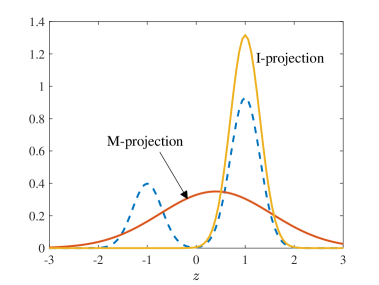
Figure 8.1: Example of I- and M-projections of a mixture of Gaussians distribution (dashed line).

Example 8.2.1.

This simple example is meant to provide an intuitive comparison between the approximations produced by I- and M-projections. To this end, consider a mixture of Gaussians distribution

$$\text{$p(z|x)=0.3\mathcal{N}$}(z|\mu_{1}=-1,\sigma_{1}^{2}=0.3)+0.7\mathcal{N}(z|\mu_{2}=1,\sigma_{2}^{2}=0.3),$$ (8.15)

as shown in Fig. 8.1. Note that this example is clearly idealized, since in practice the conditional distribution $p(z|x)$ is not known. Assume the variational distribution $q(z|\varphi)=\mathcal{N}(z|m,\gamma^{2})$ with variational parameters $\varphi=(m,\gamma^{2})$. The M-projection returns the moment matching estimates $m=\textrm{E}_{\mathrm{z\sim}p(z|x)}[\mathrm{z}]=0.4$ and $\gamma^{2}=\textrm{var}_{\mathrm{z\sim}p(z|x)}[\mathrm{z}]=0.3((\mu_{1}-m)^{2}+\sigma_{1}^{2})+0.7((\mu_{2}-m)^{2}+\sigma_{2}^{2})=1.93$ for $i=1,2.$ Instead, the I-projection can be computed numerically, yielding $m=1$ and $\gamma^{2}=0.3$. The I- and M-projections are also plotted in Fig. 8.1.

The previous example illustrates a few important facts about I- and M-projections. First, the I-projection tends to be mode-seeking and exclusive. Mathematically, this is because the variational posterior $q(z|\varphi)$ determines the support over which the distributions $p(z|x)$ and $q(z|\varphi)$ are compared by the KL divergence. Therefore, I-projections tend to underestimate the variance of a distribution. Furthermore, the I-projection is generally more accurate where $p(z|x)$ is larger. In contrast, the M-projection tends to be inclusive and to span the entire support of $p(z|x)$. This is because the M-projection prefers to avoid zero values for $q(z|\varphi)$ at values of $z$ such that $p(z|x)\neq 0$ in order to avoid an infinite KL divergence. We refer to Fig. 6.5 for a related example.

$\alpha-$Divergence.^∗ As already discussed in Sec. 6.4.3, the KL divergence is only one among many possible ways to define a measure of distance between two distributions. A metric that has found useful applications in the context of VI is the $\alpha$-divergence introduced in [minka2005divergence]. The $\alpha$-divergence between two distributions $p(x)$ and $q(x)$ is defined as

$$D_{\alpha}(p||q)=\frac{\sum_{x}\alpha p(x)+(1-\alpha)q(x)-p(x)^{\alpha}q(x)^{1-\alpha}}{\alpha(1-\alpha)},$$ (8.16)

where $p$ and $q$ need not be normalized, and $\alpha$ is a parameter. It can be proved that, as $\alpha\rightarrow 0$, we obtain $D_{\alpha}(p||q)=\textrm{KL}(q||p)$, and, when $\alpha\rightarrow 1$, we have $D_{\alpha}(p||q)=\textrm{KL}(p||q).$ Consistently with the discussion about I- and M-projections in the previous example, performing projections of the type $\textrm{min}_{\varphi}D_{\alpha}(p(x|z)||q(z|\varphi))$ with $\alpha\leq 0$ and decreasing values of $\alpha$ yields an increasingly mode-seeking, or exclusive, solution; while increasing values of $\alpha\geq 1$ yield progressively more inclusive and zero-avoiding solutions (see [minka2005divergence, Fig. 1]). Finally, for all $\alpha\neq 0$, it can be proved that the stationary points of the projection $\textrm{min}_{\varphi}D_{\alpha}(p(x|z)||q(z|\varphi))$ coincide with those of the projection $\textrm{min}_{\varphi}\textrm{KL}(p(x|z)||p(x|z)^{\alpha}q(z|\varphi)^{1-\alpha})$. The $\alpha$-divergence can be further generalized as discussed in Appendix A.

8.2.1 Mean Field Variational Inference

Mean Field VI (MFVI) is a VI method that leads to a universal, or black-box, Bayesian inference technique, such as Gibbs sampling for MC techniques. MFVI assumes the factorization $q(z)=\prod_{j}q(z_{j})$, and performs an I-projection iteratively for one hidden variable $\mathrm{z}_{i}$ at a time, while fixing the factors $q_{j}(z_{j})$ for the other latent variables $\mathrm{z}_{j}$ with $j\neq i$. No constraints are imposed on each factor $q_{j}(z_{j}).$ This corresponds to tackling the I-projection problem using block coordinate descent within the given factorized family of distributions.

For each factor $q_{i}(z_{i})$, the I-projection problem minimizes the variational free energy

$$-\textrm{E}_{\mathrm{z}_{i}\sim q_{i}(z_{i})}\left[\textrm{E}_{j\neq i}[\text{ln}p(x,\mathrm{z})]\right]-\sum_{j}H(q_{j}(z_{j})),$$ (8.17)

where we have defined for brevity the expectation

$$\textrm{E}_{j\neq i}[\text{ln}p(x,\mathrm{z})]=\textrm{E}_{\{\mathrm{z}_{j}\}_{j\neq i}\sim\prod_{j\neq i}q_{j}(z_{j})}[\text{ln}p(x,z_{i},\{\mathrm{z}_{j}\}_{j\neq i})].$$ (8.18)

Neglecting constants independent of $q_{i}(z_{i})$, this problem is equivalent to the minimization

$$\underset{q_{i}}{\text{min}}\text{ }\text{KL}(q_{i}(z_{i})||\text{exp}(\textrm{E}_{j\neq i}[\text{ln}p(x,\mathrm{z})])).$$ (8.19)

The solution to this problem can be easily seen to be obtained by normalizing the right-hand argument of the divergence as

$$q_{i}(z_{i})=\frac{\text{exp}(\textrm{E}_{j\neq i}[\text{ln}p(x,\mathrm{z})])}{\sum_{z_{i}}\text{exp}(\textrm{E}_{j\neq i}[\text{ln}p(x,\mathrm{z})])}.$$ (8.20)

MFVI solves the system of equations (8.20) for all $i$ by cycling through the factors $q_{i}(z_{i})$ or by choosing them randomly. Note that, as discussed more generally above, this procedure does not require knowledge of the desired posterior $p(z|x)$ but only of the joint distribution $p(x,z)$. The MFVI iterations are guaranteed to converge to a stationary point of the KL minimization problem.

It remains to discuss how to evaluate the expectations in (8.20). To this end, let us assume that the joint distribution $p(x,z)$ factorizes as $p(x,z)=Z^{-1}\prod_{c}\psi_{c}(x_{c},z_{c})$ as for MRFs or BNs – recall that in the latter case, we have $Z=1$. The MFVI equation (8.20) can be written as

$$q_{i}(z_{i})\propto \text{ exp}\left(\textrm{E}_{j\neq i}\left[\sum_{c}\text{ln}\psi_{c}(x_{c},\mathrm{z}_{c})\right]\right)$$ (8.21)

$$= \exp\left(\textrm{E}_{j\neq i}\left[\sum_{c:\textrm{ $z_{i}\in z_{c}$}}\text{ln}\psi_{c}(x_{c},\mathrm{z}_{c})\right]\right).$$

In the second line we have used the fact that it is sufficient to consider only the factors corresponding to cliques that include $z_{i}$. This enables implementations by means of local message passing (see, e.g., [Koller]). Furthermore, additional simplifications are possible when the factors $\psi_{c}(x_{c},z_{c})$ are log-linear, as illustrated by the next example.

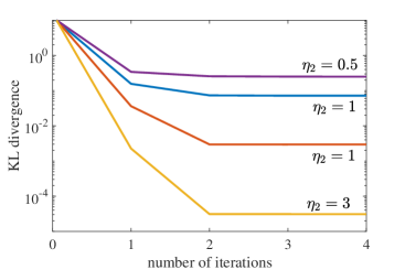
Figure 8.2: KL divergence between actual posterior and mean-field approximation as a function of the number of iterations of MFVI ($\eta_{1}=0.15$).

Example 8.2.2.

Consider again the Ising model (8.4). The MFVI equations (8.21) for approximating the posterior $p(z|x)$ are given as

$$q_{i}(z_{i})\propto \exp\Big{(}\eta_{1}\sum_{\{i,j\}}\textrm{E}_{\mathrm{z}_{j}\sim q(z_{j})}[z_{i}\mathrm{z}_{j}]+\eta_{2}x_{i}z_{i}\Big{)}$$ (8.22)

$$= \exp\Big{(}z_{i}\Big{(}\eta_{1}\sum_{\{i,j\}}\textrm{E}_{\mathrm{z}_{j}\sim q(z_{j})}[\mathrm{z}_{j}]+\eta_{2}x_{i}\Big{)}\Big{)},$$

and hence, upon normalization, we have

$$q_{i}(z_{i} =1)=\frac{1}{1+\exp(-2(\eta_{1}\sum_{\left\{i,j\right\}}\mu_{j}+\eta_{2}x_{i}))},$$ (8.23)

$$\textrm{ }=\sigma\left(2\left(\eta_{1}\sum_{\left\{i,j\right\}}\mu_{j}+\eta_{2}x_{i}\right)\right),$$

where $\mu_{i}=q_{i}(z_{i}=1)-q_{i}(z_{i}=-1)=2q_{i}(z_{i}=1)-1$.

For a numerical example, consider a $4\times 4$ binary image $\mathrm{z}$ observed as matrix $\mathrm{x}$, where the joint distribution of $\mathrm{x}$ and $\mathrm{z}$ is given by the Ising model. Note that, according to this model, the observed matrix $\mathrm{x}$ is such that each pixel of the original matrix $\mathrm{z}$ is flipped independently with probability $\sigma(-2\eta_{2})$. In this small example, it is easy to generate an image $x$ distributed according to the model, as well as to compute the exact posterior $p(z|x)$ by enumeration of all possible images $z$. The KL divergence $\textrm{KL}(p(x|z)||\prod_{i}q_{i}(z_{i}))$ obtained at the end of each iteration of MFVI – with one iteration applying (8.23) one by one to all variables – is shown in Fig. 8.2 for $\eta_{1}=0.15$ and various values of $\eta_{2}.$ As $\eta_{2}$ increases, the posterior distribution tends to become deterministic, since $x$ is an increasingly accurate measurement of $z$. As a result, the final mean-field approximation is more faithful to the real posterior, since a product distribution can capture a deterministic pmf. For smaller values of $\eta_{2},$ however, the bias due to the mean-field assumption yields a significant floor on the achievable KL divergence.

Beyond MFVI.^∗ MFVI assumes a fully factorized variational distribution $q(z)$. It is also possible to develop methods that are based on the same factorization as the joint distribution $p(x,z)$. This is known as the Bethe approach, and yields Loopy Belief Propagation (LBP) as a specific solution technique. LBP can also be interpreted as the application of message passing belief propagation, which was described in Sec. 7.4, to factor graphs with loops. Simplifications of loopy belief propagation include Approximate Message Passing (AMP). When applied to M-projections with factors restricted to lie in the exponential family, the approach yields the Expectation Propagation method. We refer to [Koller, Schniterreview] for details.

8.3 Monte Carlo-Based Variational Inference^∗

The VI methods described in the previous section require the evaluation of expectations with respect to the variational posterior (see, e.g., (8.20)). The feasibility of this operation relies on specific assumptions about the variational posterior, such as its factorization properties and membership of the exponential family. It is hence desirable to devise methods that do not require the exact computation of the ensemble averages with respect to the variational posterior $q(z|\varphi)$. As we will see below, this is possible by combining VI methods with MC approximations. The resulting methods can leverage SGD, scale to large data sets, and have found a large number of recent applications [blei2017variational, bleivariational, angelino2016patterns].

The key idea of MC-based VI is to approximate the KL divergence (8.10) via MC by drawing one or more samples $\mathrm{z}_{m}\sim$$q(z)$, with $m=1,...,M$, and by computing the empirical average

$$\textrm{KL}(q(z)||p(x,z))\simeq\frac{1}{M}\sum_{m=1}^{M}(\textrm{ln}q(z_{m})-\ln p(x,z_{m})).$$ (8.24)

In order to optimize over the parameters $\varphi$ of the variational posterior $q(z|\varphi)$, it is in fact more useful to approximate the gradient of the KL divergence, as discussed next.

REINFORCE approach. To proceed, assume the following two rather mild conditions on the parametrized variational posterior: (i) it is easy to draw samples $\mathrm{z}\sim$$q(z|\varphi)$; and (ii) it is possible to compute the gradient $\nabla_{\varphi}\textrm{ln}q(z|\varphi)$. We can now develop an SGD-based scheme as follows. The main result is that the gradient of the KL divergence in the I-projection problem (8.11) with respect to the variational parameters $\varphi$ can be written as

$$\nabla_{\varphi}\textrm{KL}(q(z|\varphi)||p(x,z))=\textrm{E}_{\mathrm{z}\sim q(z|\varphi)}\left[\nabla_{\varphi}\textrm{ln}q(\mathrm{z}|\varphi)l_{\varphi}(x,\mathrm{z})\right],$$ (8.25)

where we have defined the learning signal

$$l_{\varphi}(x,z)=\textrm{ln}q(z|\varphi)-\textrm{ln}p(x,z).$$ (8.26)

To obtain (8.25), we have used the identity $\nabla_{\varphi}\textrm{ln}q(z|\varphi)=\nabla_{\varphi}q(z|\varphi)/q(z|\varphi)$, which follows from the chain rule for differentiation, as well as the equality $\textrm{E}_{\mathrm{z}\sim q(z|\varphi)}\left[\nabla_{\varphi}\textrm{ln}q(\mathrm{z}|\varphi)\right]=0$ (see [bleivariational] for details).

MC-based VI methods evaluate an MC approximation of the gradient (8.25) at a given value $\varphi$ by drawing one or more samples $\mathrm{z}_{m}\sim$$q(z|\varphi)$, with $m=1,...,M$, and then computing

$$\nabla_{\varphi}\textrm{KL}(q(z|\varphi)||p(x,z))\simeq\frac{1}{M}\sum_{m=1}^{M}\left[\nabla_{\varphi}\textrm{ln}q(z_{m}|\varphi)l_{\varphi}(x,z_{m})\right].$$ (8.27)

This estimate is also known as likelihood ratio or REINFORCE gradient, and it can be used to update the value of $\varphi$ using SGD (see Sec. 4.1). The name reflects the origin and the importance of the approach in the reinforcement learning literature, as we briefly discuss in Chapter 9

In practice, these gradients have high variance. This is intuitively due to the fact that this estimator does not use any information about how a change in $z$ affects the learning signal $l_{\varphi}(x,z)$, since it only depends on the value of this signal. Therefore, techniques such as Rao-Blackwellization or control variates need to be introduced in order to reduce its variance (see [Yingzhen17] for a review). Simplifications are possible when the variational posterior is assumed to factorize, e.g., according to the mean-field full factorization. This approach is used in the black-box inference method of [blackbox].

Reparametrization trick. In order to mitigate the problem of the high variance of the REINFORCE estimator, the reparametrization trick leverage additional information about the dependence of the variational distribution $q(z|\varphi),$ and hence of the learning signal $l_{\varphi}(x,z)$, on the variable $z$. This approach is applicable if: (i) the latent variable $\mathrm{z}\sim q(z|\varphi)$ can be written as $\mathrm{z=}G_{\varphi}(\mathrm{w})$ for some differentiable function $G_{\varphi}(\cdot)$ and for some rv $\mathrm{w}\sim s(z)$ whose distribution does not depend on $\varphi$; and (ii) the variational regularization term $\text{KL}(q(z|\varphi)||p(z)$) in (6.12) can be computed and differentiated with respect to $\varphi$. Assumption (ii) is satisfied by members of the exponential family (see Appendix B). A typical choice that satisfies these conditions is to set $p(z)$ to be an i.i.d. Gaussian distribution; $\mathrm{w}$ as i.i.d. Gaussian rvs; and function $G_{\varphi}(w)$ as $G_{\varphi}(w)=A_{\varphi}w+b_{\varphi}$, where matrix $A_{\varphi}$ and vector $b_{\varphi}$ are parametrized by a multi-layer neural networks. Note that, with this choice, we have $q(z|\varphi)=\mathcal{N}(z|b_{\varphi},A_{\varphi}A_{\varphi}^{T})$. We refer to [jang2016categorical, maddison2016concrete] for other examples.

To see why these assumptions are useful, let us first rewrite the objective of the I-projection problem using (6.12) as

$$\textrm{KL}(q(z|\varphi)||p(x,z)) =-\textrm{E}_{\mathrm{w}\sim s(z)}\left[\textrm{ln}p(x|G_{\varphi}(\mathrm{w}))\right]+\text{KL}(q(z|\varphi)||p(z)).$$ (8.28)

We can now approximate the expectation in the first term via an empirical average by generating i.i.d. samples $\mathrm{w}_{m}\sim s(w),$ $m=1,...,M$. Note that this distribution does not depend on the current iterate $\varphi$. We can then estimate the gradient by writing

$$\nabla_{\varphi}\textrm{KL}(q(z|\varphi)||p(x,z))\simeq-\frac{1}{M}\sum_{m=1}^{M}\left[\nabla_{\varphi}\textrm{ln}p(x|G_{\varphi}(w_{m}))\right]+\nabla_{\varphi}\text{KL}(q(z|\varphi)||p(z)).$$ (8.29)

This approach tends to provide estimate with lower variance than the REINFORCE gradient, since it exploits the structure of the distribution $q(z|\varphi)$.

Both REINFORCE and reparametrization trick can be naturally combined with amortized inference. We also refer to [2017arXiv171100123G] for a proposed combination of both methods.

8.4 Approximate Learning^∗

As we have discussed, Bayesian inference plays a key role in learning problems. In this section, we briefly discuss representative schemes that incorporate approximate inference for learning. Since Bayesian learning can directly benefit from approximate inference in evaluating the posterior of the parameters and the variational posterior, we focus here on the frequentist viewpoint.

ML learning in the presence of hidden variables can be approximated by maximizing the ELBO with respect to both the model parameters $\theta$ that define the forward model $p(x|z,\theta)$ and the parameters $\varphi$ of the variational (amortized) model $q(z|x,\varphi)$. To understand what is accomplished with this optimization, it is useful to write the ELBO over a data set $\mathcal{D}$=$\{x_{n}\}_{n=1}^{N}$ using (6.14) as

$$\sum_{n=1}^{N}\ln p(x_{n}|\theta)-\text{KL}\left(q(z|x_{n},\varphi)||p(z|x_{n},\theta)\right).$$ (8.30)

As such, for any fixed $\varphi$, optimizing the ELBO over $\theta$ maximizes the likelihood function in the first term under a variational regularization term that penalizes posteriors $p(z|x,\theta)$ that are significantly different from the selected variational posteriors $q(z|x,\varphi)$. The choice of a given model for the variational posterior hence drives learning, and should be treated as model or hyperparameter selection [bloginference1].

The maximization of the ELBO over both model and variational parameters can be carried out in different ways. As a first approach, one can use EM by performing the E step via approximate inference to evaluate the posterior of the latent variables. When VI is used for this purpose, the resulting scheme is known as variational EM. Alternatively, one can use SGD with respect to both parameter vectors $\theta$ and $\varphi$ by leveraging the REINFORCE method or the reparametrization trick. The reparametrization trick approach is for instance used in the VAE method for generative modelling [VAE], also known as Deep Gaussian Latent Models [rezende2014stochastic], as well as in the black-box learning approach of [ranganath2015deep] (see also [mnih2014neural]). The KL divergence can also be substituted by an adversarially learned divergence as in the GAN approach [dumoulin2016adversarially] (see Sec. 6.4.3).

When the variational parameters are updated using an M-projection, rather than the I-projection that results from the maximization of the ELBO, the approach of jointly optimizing model and variational parameters yields the wake-sleep algorithm [hinton1995wake].

8.5 Summary

Having observed in previous chapters that learning in probabilistic models is often held back by the complexity of exact Bayesian inference for hidden variables, this chapter has provided an overview of approximate, lower-complexity, inference techniques. We have focused on MC and VI methods, which are most commonly used. The treatment stressed the impact of design choices in the selection of different types of approximation criteria, such as M- and I-projection. It also covered the use of approximate inference in learning problems. Techniques that improve over the state of the art discussed in this chapter are being actively investigated. Some additional topics for future research are covered in the next chapter.

Appendix: M-Projection with the Exponential Family

In this appendix, we consider the problem of obtaining the M-projection of a distribution $p(z)$ into a model $q(z|\varphi)=Z(\varphi)^{-1}\text{exp}(\varphi^{T}u(z))$ from the exponential family with sufficient statistics $u(z).$ We will prove that, if there exists a value of $\varphi^{*}$ of the natural parameter vector that satisfies the moment matching condition (8.14), then $q(z|\varphi^{*})$ is the M-projection.

We first write the KL divergence as

$$\text{KL}(p(z)||q(z|\varphi)) =\text{ln}Z(\varphi)-\varphi^{T}\textrm{E}_{\mathrm{z\sim}p(z)}[u(\mathrm{z})]-H(p).$$ (8.31)

The difference between the KL divergence for a generic parameter vector $\varphi$ and for the vector $\varphi^{*}$ satisfying (8.14) can be written as

$$\text{KL}(p(z)||q(z|\varphi))-\text{KL}(p(z)||q(z|\varphi^{*}))$$

$$= \text{ln$\left(\frac{Z(\varphi)}{Z(\varphi^{*})}\right)$}-(\varphi-\varphi^{*})^{T}\textrm{E}_{\mathrm{z\sim}p(z)}[u(\mathrm{z})]$$

$$= \textrm{E}_{\mathrm{z\sim}q(z|\varphi^{*})}\Bigg{[}\ln\left(\frac{q(\mathrm{z}|\varphi^{*})}{q(\mathrm{z}|\varphi)}\right)\Bigg{]}$$

$$= \text{KL}(q(z|\varphi^{*})||q(z|\varphi)).$$ (8.32)

Since the latter inequality is non-negative and equal to zero when $\varphi=\varphi^{*},$ this choice of the natural parameters minimizes the KL divergence.

Part V Conclusions

Chapter 9 Concluding Remarks

This monograph has provided a brief introduction to machine learning by focusing on parametric probabilistic models for supervised and unsupervised learning problems. It has endeavored to describe fundamental concepts within a unified treatment starting from first principles. Throughout the text, we have also provided pointers to advanced topics that we have only been able only to mention or shortly touch upon. Here, we offer a brief list of additional important aspects and open problems that have not been covered in the preceding chapters.

$\bullet$ Privacy: In many applications, data sets used to train machine learning algorithms contain sensitive private information, such as personal preferences for recommendation systems. It is hence important to ensure that the learned model does not reveal any information about the individual entries of the training set. This constraint can be formulated using the concept of differential privacy. Typical techniques to guarantee privacy of individual data points include adding noise to gradients when training via SGD and relying on mixture of experts trained with different subsets of the data [Protection].

$\bullet$ Robustness: It has been reported that various machine learning models, including neural networks, are sensitive to small variations in the data, producing the wrong response upon minor, properly chosen, changes in the explanatory variables. Note that such adversarially chosen examples, which cause a specific machine to fail, are conceptually different from the randomly selected examples that are assumed when defining the generalization properties of a network. There is evidence that finding such examples is possible even without knowing the internal structure of a machine, but solely based on black-box observations [2016arXiv160202697P]. Modifying the training procedure in order to ensure robustness to adversarial examples is an active area of research with important practical implications [goodfellow2014explaining].

$\bullet$ Computing platforms and programming frameworks: In order to scale up machine learning applications, it is necessary to leverage distributed computing architectures and related standard programming frameworks [bekkerman2011scaling, angelino2016patterns]. As a complementary and more futuristic approach, recent work has even proposed to leverage the capabilities of annealing-based quantum computers as samplers [koren2016b] or discrete optimizers [mott2017solving].

$\bullet$ Transfer learning: Machines trained for a certain task currently need to be re-trained in order to be re-purposed for a different task. For instance, a machine that learned how to drive a car would need to be retrained in order to learn how to drive a truck. The field of transfer learning covers scenarios in which one wishes to transfer the expertise acquired from some tasks to others. Transfer learning includes different related paradigms, such as multitask learning, lifelong learning, zero-shot learning, and domain adaptation [venkateswara]. In multitask learning, several tasks are learned simultaneously. Typical solutions for multitask learning based on neural networks prescribe the presence of common hidden layers among neural networks trained for different tasks [bengio2012transfer]. Lifelong learning updates a machine trained on a number of tasks to carry out a new task by leveraging the knowledge accumulated during the previous training phases [thrun1996learning]. Zero-shot learning refers to models capable of recognizing unseen classes with training examples available only for related, but different, classes. This often entails the task of learning representation of classes, such as prototype vectors, that generate data in the class through a fixed probabilistic mechanism [fu2017recent]. Domain adaptation will be discussed separately in the next point.

$\bullet$ Domain adaptation: In many learning problems, the available data has a different distribution from the data on which the algorithm will be tested. For instance, in speech recognition, one has available data for a given user at learning time, but it may be desirable, after learning, to use the same machine for another user. For supervised learning, this is typically modeled by assuming that the distribution of the covariates $\mathrm{x}$ is different during training and test, while the discriminative conditional distribution $p(t|x)$ is the same for both phases [venkateswara]. A generalization of PAC theory analyses domain adaptation, obtaining bounds on the generalization error under the desired test distribution as a function of the difference between the training and test distributions [blitzer2008learning].

$\bullet$ Communication-efficient learning: In distributed computing platforms, data is typically partitioned among the processors and communication among the processor entails latency and energy consumption. An important research problem is that of characterizing the best trade-off between learning performance and communication overhead [zhang2013info].

$\bullet$ Reinforcement learning: Reinforcement learning is at the heart of recent successes of machine learning methods in acquiring the skills necessary to play video games or games against human opponents (see, e.g., [mnih2013playing]). In reinforcement learning, one wishes to learn the optimal mapping, say $q(t|x,\theta)$, between the observed state $x$ of the world and an action $t$. Unlike supervised learning, the optimal action $t$ is not known, but the machine observes a reward/ punishment signal depending on the effect of the action. A popular approach, referred to as deep reinforcement learning, models the mapping $q(t|x,\theta)$ using a deep neural network. This is trained to maximize the average reward via SGD by using the REINFORCE method (Chapter 8) to estimate the gradient [Silverrl, Levinerl, blogRL, arulkumaran2017brief].

Appendix A Appendix A: Information Measures

In this appendix, we describe a principled and intuitive introduction to information measures that builds on inference, namely estimation and hypothesis testing. We focus on entropy, mutual information and divergence measures. We also concentrate on discrete rvs. In the monograph, we have taken the pragmatic approach of extending the definitions to continuous variables by substituting sums with integrals. It is worth noting that this approach does not come with any practical complications when dealing with mutual information and divergence. Instead, the continuous version of the entropy, known as differential entropy, should be treated with care, as it does not satisfy some key properties of the entropy such as non-negativity.

A.1 Entropy

As proposed by Claude Shannon, the amount of information received from the observation of a discrete random variable $\mathrm{x}\sim p(x)$ defined over a finite alphabet $\mathcal{X}$ should be measured by the amount of uncertainty about its value prior to its measurement [Shannon]. To this end, we consider the problem of estimating the value of $\mathrm{x}$ when one only knows the probabilistic model $p(x)$. The key idea is that the observation of a random variable $\mathrm{x}$ is more informative if its value is more difficult to predict a priori, that is, based only on the knowledge of $p(x)$.

To formalize this notion, we need to specify: (i) the type of estimates that one is allowed to make on the value of $\mathrm{x}$; and (ii) the loss function $\ell$ that is used to measure the accuracy of the estimate. We will proceed by considering two types of estimates, namely point estimates, whereby one needs to commit to a specific value $\hat{x}$ as the estimate of $\mathrm{x}$; and distributional estimates, in which instead we are allowed to produce a pmf $\hat{p}(x)$ over alphabet $\mathcal{X}$, hence defining a profile of "beliefs" over the possible values of rv $\mathrm{x}$. We will see below that the second approach yields Shannon entropy, first encountered in this monograph in (2.45).

Point Estimates. Given a point estimate $\hat{x}$ and an observed value $x\in\mathcal{\mathrm{\mathcal{X}}}$, as we have seen, the estimation error can be measured by a non-negative loss function $\ell(x,\hat{x})$, such the quadratic loss function and the 0-1 loss function. For any given loss function $\ell$, based on the discussion above, we can measure the information accrued by the observation of $\mathrm{x}\sim p_{\mathrm{x}}$ by evaluating the average loss that is incurred by the best possible a priori estimate of $\mathrm{x}$. This leads to the definition of generalized entropy [Grunwaldpaper]

$$H_{\ell}(p_{\mathrm{x}})=\min_{\hat{x}}\textrm{E${}_{\mathrm{x}\sim p_{\mathrm{x}}}$[}\ell(\mathrm{x},\hat{x})],$$ (A.1)

where the estimate $\hat{x}$ is not necessarily constrained to lie in the alphabet $\mathcal{X}$. As highlighted by the notation $H_{\ell}(p_{\mathrm{x}})$, the generalized entropy depends on the pmf $p_{\mathrm{x}}$ and on the loss function $\ell$. The notion of generalized entropy (A.1) coincides with that of minimum Bayes risk for the given loss function $\ell$.

For the quadratic loss function, the generalized entropy is the variance of the distribution $H_{\ell_{2}}(p_{\mathrm{x}})=\textrm{var}(p_{\mathrm{x}})$. To see this, impose the optimality condition $\textrm{$d$E[}(\mathrm{x}-\hat{x})^{2}]/\textrm{$d$}\hat{x}=0$ to conclude that the optimal point estimate is the mean $\hat{x}=\textrm{E}_{\mathrm{x}\sim p_{\mathrm{x}}}[\mathrm{x}].$ As for the 0-1 loss, the generalized entropy equals the minimum probability of error for the detection of $\mathrm{x}$, that is,

$$H_{\ell_{0}}(p_{\mathrm{x}})=\min_{\hat{x}}\sum_{x\neq\hat{x}}p(x)=1-\max_{\hat{x}}p(\hat{x}).$$ (A.2)

This is because the optimal estimate is the mode, i.e., the value $\hat{x}$ with the largest probability $p(\hat{x})$.

Distributional Estimate. We now consider a different type of estimation problem in which we are permitted to choose a pmf $\hat{p}(x)$ on the alphabet $\mathcal{X}$ as the estimate for the outcome of variable $\mathrm{x}$. To facilitate intuition, we can imagine $\hat{p}(x)$ to represent the fraction of one’s wager that is invested on the outcome of $\mathrm{x}$ being a specific value $x$. Note that it may not be necessarily optimal to put all of one’s money on one value $x$! In fact, this depends on how we measure the reward, or conversely the cost, obtained when a value $\mathrm{x}=x$ is realized.

To this end, we define a non-negative loss function $\ell(x,\hat{p}_{\mathrm{x}})$ representing the loss, or the “negative gain”, suffered when the value $\mathrm{x}=x$ is observed. This loss should sensibly be a decreasing function of $\hat{p}(x)$ – we register a smaller loss, or conversely a larger gain, when we have wagered more on the actual outcome $x$. As a fairly general class of loss functions, we can hence define

$$\ell(x,\hat{p}_{\mathrm{x}})=f(\hat{p}(x)),$$ (A.3)

where $f$ is a decreasing function. More general classes of loss functions are considered in [DeGroot].

Denote as $\Delta(\mathcal{\mathcal{X}})$ the simplex of pmfs defined over alphabet $\mathcal{X}$. The generalized entropy can now be defined in a way that is formally equivalent to (A.1), with the only difference being the optimization over pmf $\hat{p}_{\mathrm{x}}$ rather than over point estimate $\hat{x}$:

$$H_{\ell}(p_{\mathrm{x}})=\min_{\hat{p}_{\mathrm{x}}\in\Delta(\mathcal{\mathcal{X}})}\textrm{E${}_{\mathrm{x}\sim p_{\mathrm{x}}}$[}\ell(\mathrm{x},\hat{p}_{\mathrm{x}})].$$ (A.4)

A key e$\mathrm{x}$ample of loss function $\ell(x,\hat{p}_{\mathrm{x}})$ in class (A.3) is the log-loss $\ell(x,\hat{p}_{\mathrm{x}})=-\log\hat{p}(x)$. The log-loss has a strong motivation in terms of lossless compression. In fact, as discussed in Sec. 2.5, by Kraft’s inequality, it is possible to design a prefix-free – and hence decodable without delay – lossless compression scheme that uses $\left\lceil-\log\hat{p}(x)\right\rceil$ bits to represent value $x$. As a result, the choice of a pmf $\hat{p}_{\mathrm{x}}$ is akin to the selection of a prefix-free lossless compression scheme that requires a description of around $-\ln\hat{p}(x)$ bits to represent value $x$. The expectation in (A.4) measures the corresponding average number of bits required for lossless compression by the given scheme.

Using the log-loss in (A.1), we obtain the Shannon entropy

$$\min_{\hat{p}_{\mathrm{x}}\in\Delta(\mathcal{\mathcal{X}})}\textrm{E${}_{\mathrm{x}\sim p_{\mathrm{x}}}$$[-$$\ln$$\hat{p}(\mathrm{x})$}],$$ (A.5)

$$=\textrm{E${}_{\mathrm{x}\sim p_{\mathrm{x}}}$$[-$$\ln$$p(\mathrm{x})$}]=H(p_{\mathrm{x}}).$$ (A.6)

In fact, imposing the optimality condition yields the optimal pmf $\hat{p}(x)$ as $\hat{p}(x)=p(x)$. Equation (A.5) reveals that the entropy $H(p_{\mathrm{x}})$ is the minimum average log-loss when optimizing over all possible pmfs $\hat{p}_{\mathrm{x}}$.

It may seem at first glance that the choice $\hat{p}(x)=p(x)$ should be optimal for most reasonable loss functions in class (A.3), but this is not the case. In fact, when the alphabet $\mathcal{X}$ has more than two elements, it can be proved that the log-loss – more generally defined as $\ell(x,\hat{p}_{\mathrm{x}})=b\log\hat{p}(x)+c$ with $b\leq 0$ and any $c$ – is the only loss function of the form (A.3) for which $\hat{p}(x)=p(x)$ is optimal [Weissmanarxiv].

As a final note, the generalized entropy $H_{\ell}(p_{\mathrm{x}})$ is a concave function of $p_{\mathrm{x}}$, which means that we have the inequality $H_{\ell}(\lambda p_{\mathrm{x}}+(1-\lambda)q_{\mathrm{x}})\geq\lambda H_{\ell}(p_{\mathrm{x}})+(1-\lambda)H_{\ell}(q_{\mathrm{x}})$ for any two distributions $p_{\mathrm{x}}$ and $q_{\mathrm{x}}$ and any $0\leq\lambda\leq 1$. This follows from the fact that the entropy is the minimum over a family of linear functionals of $p_{\mathrm{x}}$ [Boyd]. The concavity of $H_{\ell}(p_{\mathrm{x}})$ implies that a variable $\mathrm{x}\sim\lambda p_{\mathrm{x}}+(1-\lambda)q_{\mathrm{x}}$ distributed according to the mixture of two distributions is more “random”, i.e., it is more difficult to estimate, than both variables $\mathrm{x}\sim p_{\mathrm{x}}$ and $\mathrm{x}\sim q_{\mathrm{x}}$.

A.2 Conditional Entropy and Mutual Information

Given two random variables $\mathrm{x}$ and $\mathrm{y}$ jointly distributed according to a known probabilistic model $p(x,y)$, i.e., $(\mathrm{x},\mathrm{y})\sim p_{\mathrm{xy}}$, we now discuss how to quantify the information that the observation of one variable, say $\mathrm{y}$, brings about the other, namely $\mathrm{x}$. Following the same approach adopted above, we can distinguish two inferential scenarios for this purpose: in the first, a point estimate $\hat{x}(y)$ of $\mathrm{x}$ needs to be produced based on the observation of a value $\mathrm{y}=y$ and the knowledge of the joint pmf $p_{\mathrm{x}\mathrm{y}}$; while, in the second, we are allowed to choose a pmf $\hat{p}_{\mathrm{x}|\mathrm{y}=y}$ as the estimate of $\mathrm{x}$ given the observation $\mathrm{y}=y.$

Point Estimate: Assuming point estimates and given a loss function $\ell(x,\hat{x})$, the generalized conditional entropy for an observation $\mathrm{y}=y$ is defined as the minimum average loss

$$H_{\ell}(p_{\mathrm{x}|\mathrm{y}=y})=\min_{\hat{x}(y)}\textrm{E${}_{\mathrm{x}\sim p_{\mathrm{x}|\mathrm{y}=y}}$[}\ell(\mathrm{x},\hat{x}(y))|\mathrm{y}=y].$$ (A.7)

Note that this definition is consistent with (A.1) as applied to the conditional pmf $p_{\mathrm{x}|\mathrm{y}=y}$. Averaging over the distribution of the observation $\mathrm{y}$ yields the generalized conditional entropy

$$H_{\ell}(\mathrm{x}|\mathrm{y})=\textrm{E}_{\mathrm{y}\sim p_{\mathrm{y}}}[H_{\ell}(p_{\mathrm{x}|\mathrm{y}})].$$ (A.8)

It is emphasized that the generalized conditional entropy depends on the joint distribution $p_{\mathrm{x}\mathrm{y}}$, while (A.7) depends only on the conditional pmf $p_{\mathrm{x}|\mathrm{y}=y}$.

For the squared error, the generalized conditional entropy can be easily seen to be the average conditional variance $H_{\ell_{2}}(\mathrm{x}|\mathrm{y})=\textrm{E}_{\mathrm{y}\sim p_{\mathrm{y}}}[\textrm{var}$$(p_{\mathrm{x}|\mathrm{y}})$], since the a posteriori mean $\hat{x}(y)=\textrm{E}_{\mathrm{x}\sim p_{\mathrm{x}|\mathrm{y}=y}}[\mathrm{x}|\mathrm{y}=y]$ is the optimal estimate. For the 0-1 loss, the generalized conditional entropy $H_{\ell_{0}}(\mathrm{x}|\mathrm{y})$ is instead equal to the minimum probability of error for the detection of $\mathrm{x}$ given $\mathrm{y}$ and the MAP estimate $\hat{x}(y)=\textrm{argmax}_{\hat{x}\in\mathcal{\mathrm{x}}}p(\hat{x}|y)$ is optimal.

Distributional Estimate: Assume now that we are allowed to choose a pmf $\hat{p}_{\mathrm{x}|\mathrm{y}=y}$ as the estimate of $\mathrm{x}$ given the observation $\mathrm{y}=y$, and that we measure the estimation loss via a function $\ell(x,\hat{p}_{\mathrm{x}})$ as in (A.3). The definition of generalized conditional entropy for a given value of $\mathrm{y}=y$ follows directly from the arguments above and is given as $H_{\ell}(p_{\mathrm{x}|\mathrm{y}=y})$, while the generalized conditional entropy is (A.8). With the log-loss function, the definition above can be again seen to coincide with Shannon conditional entropy $H(\mathrm{x}|\mathrm{y})=\textrm{E${}_{\mathrm{x},\mathrm{y}\sim p_{\mathrm{x},\mathrm{y}}}$[}-\ln p(\mathrm{x}|\mathrm{y})]$.

If $\mathrm{x}$ and $\mathrm{y}$ are independent, we have the equality $H_{\ell}(\mathrm{x}|\mathrm{y})=H_{\ell}(\mathrm{x})$. Furthermore, since in (A.7) we can always choose estimates that are independent of $\mathrm{y}$, we generally have the inequality $H_{\ell}(\mathrm{x}|\mathrm{y})\leq H_{\ell}(\mathrm{x})$: observing $\mathrm{y}$, on average, can only decrease the entropy. Note, however, that it is not true that $H_{\ell}(p_{\mathrm{x}|\mathrm{y}=y})$ is necessarily smaller than $H_{\ell}(\mathrm{x})$ [Cover].

Mutual Information: The inequality $H_{\ell}(\mathrm{x}|\mathrm{y})\leq H_{\ell}(\mathrm{x})$ justifies the definition of generalized mutual information with respect to the given loss function $\ell$ as

$$I_{\ell}(\mathrm{x};\mathrm{y})=H_{\ell}(\mathrm{x})-H_{\ell}(\mathrm{x}|\mathrm{y}).$$ (A.9)

The mutual information measures the decrease in average loss that is obtained by observing $\mathrm{y}$ as compared to having only prior information about $p_{\mathrm{x}}$. This notion of mutual information is in line with the concept of statistical information proposed by DeGroot (see [DeGroot] for a recent treatment). With the log-loss, the generalized mutual information (A.9) reduces to Shannon’s mutual information. As shown in [jiao2015justification], the log-loss is in fact the only loss function, up to multiplicative factors, under which the generalized mutual information (A.9) satisfies the data processing inequality, as long as the alphabet of $\mathrm{x}$ has more than two elements.

A.3 Divergence Measures

We now discuss a way to quantify the “difference” between two given probabilistic models $p_{\mathrm{x}}$ and $q_{\mathrm{x}}$ defined over the same alphabet $\mathcal{X}.$ We consider here the viewpoint of binary hypothesis testing as a theoretical framework in which to tackle the issue. Other related approaches have also found applications in machine learning, including optimal transport theory and kernel methods [Wasserstein].

We consider the following standard binary hypothesis testing problem. Given an observation $\mathrm{x}$, decide whether $\mathrm{x}$ was generated from pmf $p_{\mathrm{x}}$ or from pmf $q_{\mathrm{x}}.$ To proceed, we define a decision rule $T(x)$, which should have the property that it is increasing with the certainty that a value $\mathrm{x}=x$ is generated from $p_{\mathrm{x}}$ rather than $q_{\mathrm{x}}$. For e$\mathrm{x}$ample, in practice, one may impose a threshold on the rule $T(x)$ so that, when $T(x)$ is larger than the threshold, a decision is made that $\mathrm{x}=x$ was generated from $p_{\mathrm{x}}$.

In order to design the decision rule $T(x)$, we again minimize a loss function or, equivalently, maximize a merit function. For convenience, here we take the latter approach, and define the problem of maximizing the merit function

$$\textrm{E}_{\mathrm{x}\sim p_{\mathrm{x}}}[T(\mathrm{x})]-\textrm{E}_{\mathrm{x}\sim q_{\mathrm{x}}}[g(T(\mathrm{x}))]$$ (A.10)

over the rule $T(x)$, where $g$ is a concave increasing function. This criterion can be motivated as follows: (i) It increases if $T(\mathrm{x})$ is large, on average, for values of $\mathrm{x}$ generated from $p_{\mathrm{x}}$; and (ii) it decreases if, upon expectation, $T(\mathrm{x})$ is large for values of $\mathrm{x}$ generated from $q_{\mathrm{x}}.$ The function $g$ can be used to define the relative importance of errors made in favor of one distribution or the other. From this discussion, the optimal value of (A.10) can be taken to be a measure of the distance between the two pmfs. This yields the following definition of divergence between two pmfs

$$D_{f}(p_{\mathrm{x}}||q_{\mathrm{x}})=\max_{T(x)}\textrm{ E}_{\mathrm{x}\sim p_{\mathrm{x}}}[T(\mathrm{x})]-\textrm{E}_{\mathrm{x}\sim q_{\mathrm{x}}}[g(T(\mathrm{x}))],$$ (A.11)

where the subscript $f$ will be justified below.

Under suitable differentiability assumptions on function $g$ (see [fGAN] for generalizations), taking the derivative with respect to $T(x)$ for all $x\in\mathcal{\mathrm{\mathcal{\mathrm{x}}}}$ yields the optimality condition $g^{\prime}(T(x))=p(x)/q(x)$. This relationship reveals the connection between the optimal detector $T(x)$ and the LLR $p(x)/q(x)$. Plugging this result into (A.11), it can be directly checked that the following equality holds [Nguyen]

$$D_{f}(p_{\mathrm{x}}||q_{\mathrm{x}})=\textrm{E}_{\mathrm{x}\sim q_{\mathrm{x}}}\left[f\left(\frac{p_{\mathrm{x}}(\mathrm{x})}{q_{\mathrm{x}}(\mathrm{x})}\right)\right],$$ (A.12)

where the function $f(x)=g^{*}(x)$ is the convex dual function of $g(t)$, which is defined as $g^{*}(x)=\sup_{t}\left(xt-g(t)\right)$. Note that dual function $f$ is always convex [Boyd].

Under the additional constraint $f(1)=0$, definition (A.12) describes a large class of divergence measures parametrized by the convex function $f$, which are known as $f$-divergences or Ali-Silvey distance measures [Duchicourse]. Note that the constraint $f(1)=0$ ensures that the divergence is zero when the pmfs $p_{\mathrm{x}}$ and $q_{\mathrm{x}}$ are identical. Among their key properties, $f$-divergences satisfy the data processing inequality [Duchicourse].

For e$\mathrm{x}$ample, the choice $g(t)=\exp(t-1)$, which gives the dual convex $f(x)=x\ln x$, yields the optimal detector $T(x)=1+\ln(p(x)/q(x))$ and the corresponding divergence measure (A.12) is the standard KL divergence KL$(p_{\mathrm{x}}||q_{\mathrm{x}})$. As another instance of $f$-divergence, with $g(t)=-\ln(2-\exp(t))$ we obtain the optimal detector $T(x)=\ln(2p_{\mathrm{x}}(x)/p_{\mathrm{x}}(x)+q_{\mathrm{x}}(x))$, and $D_{f}(p_{\mathrm{x}}||q_{\mathrm{x}})$ becomes the Jensen-Shannon divergence. For reference, the latter can be written as

$$\textrm{JS}(p_{\mathrm{x}}||q_{\mathrm{x}})=\textrm{ KL$\left(p_{\mathrm{x}}\parallel m_{\mathrm{x}}\right)$+KL$\left(q_{\mathrm{x}}\parallel m_{\mathrm{x}}\right)$},$$ (A.13)

where $m_{\mathrm{x}}(x)=(p_{\mathrm{x}}(x)+q_{\mathrm{x}}(x))/2.$ Another special case, which generalizes the KL divergence and other metrics, is the $\alpha$-divergence discussed in Chapter 8 (see (8.16)), which is obtained with $f(x)=(\alpha(x-1)-(x^{\alpha}-1))/(\alpha(1-\alpha))$ for some real-valued parameter $\alpha$. We refer to [fGAN, Duchicourse] for other examples.

The discussion above justified the adoption of the loss function (A.11) in a heuristic fashion. It is, however, possible to derive formal relationships between the error probability of binary hypothesis testing and f-divergences [Berisha]. We also refer to the classical Sanov lemma and Stein lemma as fundamental applications of KL divergence to large deviation and hypothesis testing [Cover].

Appendix B Appendix B: KL Divergence and Exponential Family

In this appendix, we provide a general expression for the KL divergence between two distributions $p(x|\eta_{1})$ and $p(x|\eta_{2})$ from the same regular exponential family with log-partition function $A(\cdot)$, sufficient statistics $u(x)$, and moment parameters $\mu_{1}$ and $\mu_{2}$, respectively. We recall from Chapter 3 that the log-partition function is convex and that we have the identity $\nabla A(\eta)=\mu.$

The KL divergence between the two distributions can be translated into a divergence on the space of natural parameters. In particular, the following relationship holds [Amari]

$$\textrm{KL}(p(x|\eta_{1})||p(x|\eta_{2}))=D_{A}(\eta_{2},\eta_{1}),$$ (B.1)

where $D_{A}(\eta_{2},\eta_{1})$ represents the Bregman divergence with generator function given by the log-partition function $A(\cdot)$, that is

$$D_{A}(\eta_{2},\eta_{1}) =A(\eta_{2})-A(\eta_{1})-(\eta_{2}-\eta_{1})^{T}\nabla A(\eta_{1})$$

$$=A(\eta_{2})-A(\eta_{1})-(\eta_{2}-\eta_{1})^{T}\mu_{1}.$$ (B.2)

The first line of (B.2) is the general definition of the Bregman divergence $D_{A}(\cdot,\cdot)$ with a generator function $A(\cdot),$ while the second follows from the relationship (3.10). Note that the Bregman divergence can be proved to be non-negative, and convex in its first argument, but not necessarily in the second argument. The equality (B.1)-(B.2) can be proved by using the definition of exponential family via the following equality

$$\textrm{KL}(p(x|\eta_{1})||p(x|\eta_{2})) =\textrm{E}_{\mathrm{x}\sim p(x|\eta_{1})}\left[\log\frac{p(\mathrm{x}|\eta_{1})}{p(\mathrm{x}|\eta_{2})}\right]$$

$$=\textrm{E}_{\mathrm{x}\sim p(x|\eta_{1})}[(\eta_{1}-\eta_{2})^{T}u(\mathrm{x})]-A(\eta_{1})+A(\eta_{2}).$$ (B.3)

Recalling again that we have the equality $\nabla A(\eta_{1})=\mu_{1}$, the relationship (B.1)-(B.2) can be approximated as

$$\begin{split}\textrm{KL}(p(x|\eta_{1})||p(x|\eta_{2}))&=\frac{1}{N}(\eta_{1}-\eta_{2})^{T}J_{\eta_{1}}(\eta_{1}-\eta_{2})+O(||\eta_{1}-\eta_{2}||^{3})\end{split},$$ (B.4)

where $J_{\eta}=-\text{E}\left[\nabla_{\eta}^{2}\text{ln}p(\mathrm{x}|\eta)\right]$ is the Fisher information matrix. This expansion holds given the relationship $\nabla_{\eta}^{2}A(\eta)=J_{\eta}$ [Duchicourse].

It is also possible to write a relationship analogous to (B.1)-(B.2) in terms of mean parameters. This is done by using the convex conjugate function

$$A^{*}(\mu)=\sup_{\eta}\eta^{T}\mu-A(\eta),$$ (B.5)

where the maximization is over the feasible set of natural parameters. In fact, the optimization over $\eta$ yields the natural parameter $\eta$ corresponding to the mean parameter $\mu$, i.e., $\nabla A(\eta)=\mu$. It hence follows from (B.2) that we have

$$\textrm{KL}(p(x|\mu_{1})||p(x|\mu_{2})) =A^{*}(\mu_{1})-A^{*}(\mu_{2})-(\mu_{1}-\mu_{2})^{T}\eta_{2}$$

$$=D_{A^{*}}(\mu_{1},\mu_{2}),$$ (B.6)

where in the second line we have used the inverse mapping $\nabla A*(\mu)=\eta$ between mean and natural parameters (which holds for minimal families).

Chernoff divergence measures, including the Bhattacharyya distance, can also be written in closed form for exponential families [Nielsen].