Probing new spin-independent interactions through precision spectroscopy in atoms with few electrons

Abstract

The very high precision of current measurements and theory predictions of spectral lines in few-electron atoms allows to efficiently probe the existence of exotic forces between electrons, neutrons and protons. We investigate the sensitivity to new spin-independent interactions in transition frequencies (and their isotopic shifts) of hydrogen, helium and some helium-like ions. We find that present data probe new regions of the force-carrier couplings to electrons and neutrons around the MeV mass range. We also find that, below few keV, the sensitivity to the electron coupling in precision spectroscopy of helium and positronium is comparable to that of the anomalous magnetic moment of the electron. Finally, we interpret our results in the dark-photon model where a new gauge boson is kinetically mixed with the photon. There, we show that helium transitions, combined with the anomalous magnetic moment of the electron, provide the strongest indirect bound from laboratory experiments above $100\,$keV.

I Introduction

Fundamental interactions of known elementary particles are well described by the the Standard Model (SM) of particle physics. Nevertheless, the SM cannot be the complete description of Nature since it does not account for neutrino oscillations, does not provide a viable dark matter candidate and cannot explain the baryon asymmetry of the Universe. Moreover, the SM suffers from several hierarchy problems, such as the stability of the Higgs mass to quantum corrections and the strong CP problem. In addition, it contains intriguing puzzles related to the observed large hierarchies in the charged fermion masses and quark mixing angles. However, non of these pending issues which call for new physics (NP) beyond the SM indicate a specific energy scale at which the associated NP phenomena will manifest themselves. Hence, a broad experimental program must be pursued.

While accelator-based experiments search directly for new particles over many orders of the mass and couplings, precision low-energy measurements may also reveal indirectly in a complementary approach the existence of new phenomena. Precise atomic physics table-top experiments are promising in this regard. For example, observables which violate discrete symmetries of QED, as in parity-violating transitions Porsev:2009pr ; Tsigutkin:2009zz ; PhysRevA.81.032114 ; Leefer:2014tga ; Versolato:2011zza ; Dzuba:2012kx ; Roberts:2014bka ; Jungmann:2014kia , are a powerful tool to probe NP Agashe:2014kda .

Parity-conserving transitions are also interesting probes of NP which, however, require higher theoretical control. Frequency measurements of narrow atomic transitions in heavy elements are possible within a few$\times 10^{-16}$ relative accuracy PhysRevLett.113.210801 ; PhysRevLett.108.090801 thanks to the optical frequency comb technique PhysRevLett.84.3232 ; REICHERT199959 . Moreover, the experimental uncertainty in some systems now reaches the $10^{-18}$ level PhysRevLett.116.063001 ; Bloom:2013uoa , thus indicating the possibility of significant improvement in the near future. A limitation in translating the experimental precision to a bound on NP is the theory uncertainty, which is by far larger than the experimental precision. However, the high accuracy achieved in frequency measurements of narrow atomic transitions in heavy elements can be exploited to probe NP provided new observables largely insensitive to theory uncertainties are identified. For example, Refs. Delaunay:2016brc ; Frugiuele:2016rii ; Delaunay:2016zmu ; Berengut:2017zuo proposed to bound new interactions between neutrons and electrons by testing linearity of King plots King:63 of isotope shift (IS) measurements.

The situation is different for atoms and ions with few electrons and a small number of nucleons. There, QED calculations are carried out to high accuracy. For instance, low excited states in helium can be calculated up to $\mathcal{O}(\alpha^{6})$ corrections, which yields theoretical predictions often more accurate than the measurements, see e.g. Refs. Pachucki:2017xcg ; Karshenboim:2000kv . In addition, nuclear finite size effects are also well described thanks to the extraction of the nuclear radius from electron scattering experiments and muonic atom spectroscopy. This allows to directly compare theory and experiment in order to probe NP interactions Karshenboim:2010ck ; Karshenboim:2010cg ; Jaeckel:2010xx ; Ficek:2016qwp .

In this work we derive new limits on spin-independent NP interactions between the proton/neutron and the electron from optical frequency measurements, as well as from frequency shifts between different isotopes, in hydrogen and helium atoms, helium-like ions such as lithium and nitrogen. In addition, we constrain new electron-electron interactions via precision spectroscopy of helium and positronium atoms. We compare the resulting bounds on the product of the electron and neutron couplings and on the electron coupling separately, with existing indirect constraints and future prospects from IS measurement in heavier systems with many electrons. Furthermore, we perform global fits using all available transitions to constrain simultaneously the electron, neutron and proton couplings in a model-independent way. Finally, as a phenomenological application, we interpret the bounds within the dark photon model.

II Constraining new spin-independent interactions in atoms

Consider a new force mediated by a boson $\phi$ of mass $m_{\phi}$ and spin $s=0,1,2$ with spin-independent couplings to the electron, proton and neutron $y_{e}$, $y_{p}$ and $y_{n}$, respectively. At atomic energies, the exchange of $\phi$ is described by an effective potential between a nucleus $N$ of charge $Z$ and mass number $A$ and its bound electrons as

$$V_{N}(r)=\frac{(-1)^{s+1}}{4\pi}y_{e}y_{N}\frac{e^{-m_{\phi}r}}{r}\,,$$ (1)

where $y_{N}\equiv y_{p}Z+(A-Z)y_{n}$ and $r$ is the electron-nucleus distance.

For atoms with more than one electron, like helium, an effective potential between electron pairs is also induced

$$V_{e}(r_{12})=(-1)^{s+1}\frac{y_{e}^{2}}{4\pi}\frac{e^{-m_{\phi}r_{12}}}{r_{12}}\,,$$ (2)

where $r_{12}\equiv|\vec{r}_{1}-\vec{r}_{2}|$ is the distance between electron $1$ and electron $2$, with $\vec{r_{1}}$, $\vec{r_{2}}$ describing their positions relative to the nucleus.

The total frequency shift induced by the above potentials for a transition $i$ between atomic states $a$ and $b$ (with $E_{b}>E_{a}$) is described by first-order perturbation theory as

$$\delta_{\rm NP}\nu^{A}_{i}=(-1)^{s+1}\left(y_{e}y_{N}X_{i}+y_{e}^{2}Y_{i}\right)\,,$$ (3)

where $X_{i}$ and $Y_{i}$ are overlap integrals with the electronic wavefunctions depending only on the $\phi$ boson mass. In this paper, we focus on electronic transitions in helium-like and hydrogen atoms, for which the $X_{i}$ and $Y_{i}$ functions are calculated within first-order perturbation theory using non-relativistic wavefunctions as detailed in Appendices B and C. While QED calculations rely on much more sophisticated wavefunctions, the use of the non-relativistic ones is a sufficient approximation to the dominant NP effects. Helium wavefunctions are very well approximated by antisymmetrized combinations of hydrogenic wavefunctions with effective nuclear charges accounting for the electronic screening Eckart , except for the $2S$ spin-singlet state where an accurate description of the inter-electron repulsion requires the use of Hylleraas functions Hylleraas1928 ; Hylleraas1929 .

Taking into account the NP contribution in Eq. (3), the theory prediction for the frequency of an electronic transition $i$ in an isotope $A$ is given by

$$\nu^{A}_{i}= \nu^{A}_{i,0}+F_{i}\langle r^{2}\rangle_{A}+\delta_{\rm NP}\nu^{A}_{i}\,,$$ (4)

where $\nu^{A}_{i,0}$ is the dominant contribution calculated in the point-like nucleus limit (including spin effects and nuclear polarizability), whereas the second term describes the leading finite nuclear size effects, $\langle r^{2}\rangle_{A}$ being the nuclear charge radius squared and $F_{i}$ is the field-shift (FS) constant. The IS between two isotopes $A$ and $A^{\prime}$ for this transition is then described as

$$\nu^{A,A^{\prime}}_{i}=\nu^{A,A^{\prime}}_{i,0}+F_{i}\delta\langle r^{2}\rangle_{A,A^{\prime}}+y_{e}y_{n}X_{i}(A-A^{\prime})\,,$$ (5)

where $\nu^{A,A^{\prime}}_{i}\equiv\nu^{A}_{i}-\nu_{i}^{A^{\prime}}$ and $\delta\langle r^{2}\rangle_{A,A^{\prime}}\equiv\langle r^{2}\rangle_{A}-\langle r^{2}\rangle_{A^{\prime}}$. Higher-order effects of nuclear charge radius and finite magnetic radius are not resolvable by the current experimental accuracy Pachucki:2017xcg ; 2015JPCRD..44c1206P and are therefore omitted in Eqs. (4) and (5).

Absolute frequencies and IS in hydrogen and helium are calculated to high accuracy in the limit of point-like nuclei. However, the full theoretical prediction is often limited by the uncertainty related to the finite nuclear size effects. For a comparison between the experimental value and the QED prediction in the point-nucleus limit, we define

$$\Delta^{A}_{i}\equiv\nu_{i,{\rm exp}}^{A}-\nu_{i,{0}}^{A}\,.$$ (6)

The NP contribution generically depends on the three coupling constants, $y_{e}$, $y_{p}$, and $y_{n}$, and the mediator mass, $m_{\phi}$. At fixed $m_{\phi}$ the product $y_{e}y_{n}$ can be probed independently of $y_{p}$ from a single IS measurement (for any transition $i$) using Eq. (5)

$$y_{e}y_{n}=\frac{\Delta^{A,A^{\prime}}_{i}-F_{i}\delta\langle r^{2}\rangle_{A,A^{\prime}}}{X_{i}(A-A^{\prime})}\,,$$ (7)

where $\Delta_{i}^{A,A^{\prime}}\equiv\Delta_{i}^{A}-\Delta_{i}^{A^{\prime}}$ using Eq. (6). Hence the NP bound depends on the change in the mean-square nuclear charge radius, $\delta\langle r^{2}\rangle_{A,A^{\prime}}$, which is measured either in electron scattering or in muonic atom spectroscopy experiments. Whenever applicable, the latter typically yields much more precise values of the charge radii. In principle, the charge radius determination via electron scattering may be affected by NP. However, we find that NP is only noticeable there for large coupling values that are already excluded by more sensitive probes. Hence the charge radius extraction from electron scattering cannot be contaminated by NP. Muonic atom spectroscopy measurements are more sensitive to NP contributions, especially in the keV–MeV mass range, and existing constraints on the $y_{\mu}y_{n}$ coupling product do not rule out the possibility of NP contaminations in this region Liu:2016qwd ; TuckerSmith:2010ra ; Beltrami:1985dc . Therefore, for simplicity we will henceforth assume $y_{\mu}=0$.

Alternatively, the charge radius dependence can be eliminated using an IS measurement in a second transition, yielding

$$y_{e}y_{n}=\frac{F_{2}\Delta_{1}^{A,A^{\prime}}-F_{1}\Delta_{2}^{A,A^{\prime}}}{(F_{2}X_{1}-F_{1}X_{2})(A-A^{\prime})}\,,$$ (8)

which, besides $X_{1,2}$, depends only on quantities known theoretically with high accuracy, namely $F_{2}/F_{1}$ and $\nu_{i,0}^{A,A^{\prime}}$. The main drawback of Eq. (8) relative to Eq. (7) is the possible loss of sensitivity when $(F_{2}X_{1}-F_{1}X_{2})\to 0$ Delaunay:2016brc ; Berengut:2017zuo . The latter is rather severe for all $m_{\phi}$ when close-by transitions with $F_{1}\approx F_{2}$ and $X_{1}\approx X_{2}$ are used, for example in transitions involving different states of the same fine-structure multiplet. Another disadvantage of Eq. (8) is represented by how rapidly the sensitivity to $y_{e}y_{n}$ weakens at large mass. While $X_{i}\propto m_{\phi}^{-2}$ above $m_{\phi}\sim\mathcal{O}(10\,$keV), this leading term cancels out in the difference $(F_{2}X_{1}-F_{1}X_{2})\propto m_{\phi}^{-3}$ Berengut:2017zuo . Equation (8) bears resemblance to the method proposed in Ref. Berengut:2017zuo for heavy elements. However, there, the less accurate theory calculations for $\nu_{i,0}^{A,A^{\prime}}$ are traded for IS measurements between two additional isotope pairs.

NP contributions to the electron-electron and electron-proton interactions cancel out to first approximation in the IS. Thus, they can be probed more efficiently in absolute frequency measurements, despite the lower absolute accuracy. Helium transitions are sensitive to both kinds of interaction. In fact a combination of two frequency measurements can resolve the $y_{e}y_{N}$ and $y_{e}^{2}$ coupling products, thanks to transition-dependent $X_{i},Y_{i}$ constants in Eq. (3). Hydrogen frequencies are sensitive to electron-proton interactions and have been used previously to probe $y_{e}y_{p}$ Karshenboim:2010ck ; Karshenboim:2010cg ; Jaeckel:2010xx . However, presently unresolved issues related to the well-known proton radius puzzle protonsize ; protonsize2 limits the application of hydrogen spectroscopy for constraining new atomic forces. Therefore, we will not use absolute spectroscopy measurements of hydrogen or deuterium as a probe of NP. Instead, we will consider hydrogen-deuterium IS spectroscopy since in this case there is no tension between $\delta\langle r^{2}\rangle$ values extracted from electronic and muonic measurements Pohl1:2016xoo .

III Bounds from Isotope shift measurements

Let us first discuss probes of new electron-neutron interactions. We focus here on spectroscopic probes based on IS measurements in helium, helium-like and hydrogen/deuterium atoms. The comparison of theory to experiment directly probes $y_{e}y_{n}$ independently of the presence of a NP coupling to protons. As shown in Table 1 (a full list of our input values is given in Appendix A), the theory uncertainty (in the point-like nucleus limit) is currently smaller than the experimental error for transitions involving low excited states, and the sensitivity to NP is limited by the experimental determination of charge radius differences. Our results are summarized in Fig. 1 which show the best constraints on $y_{e}y_{n}$, as a function of the mediator mass, arising from transitions in hydrogen and helium(-like) atoms.

For comparison, we also show constraints derived from King linearity in heavy atoms Berengut:2017zuo and from other (non-atomic) observables. Those include laboratory constraints resulting from the anomalous magnetic moment of the electron $a_{e}\equiv(g-2)_{e}/2$ Olive:2016xmw ; Hanneke:2010au , neutron scattering on atomic electrons Adler:1974ge or nuclei Barbieri:1975xy ; Leeb:1992qf ; Nesvizhevsky:2007by ; Pokotilovski:2006up and fifth force experiments Bordag:2001qi ; bordag2009advances , as well as astrophysical constraints from SN 1987a Raffelt:2012sp and globular clusters  Yao:2006px ; Grifols:1986fc ; Grifols:1988fv ; Hardy:2016kme ; Redondo:2013lna . Note that also spectroscopy in molecular ions and antiprotonic helium constrains spin-independent interactions of nucleons Salumbides:2013dua ; Ubachs:2015fuf ; Biesheuvel2016 ; UBACHS20161 , but it results in weaker bounds than from neutron scattering and is therefore not shown in Fig. 1. Some of these constraints can be evaded in specific models Feldman:2006wg ; Nelson:2008tn ; Burrage:2007ew ; Burrage:2016bwy ; Brax:2010gp . We notice that bounds from few-electron atoms provide the strongest (indirect) constraints in the region above 300 keV where astrophysical bounds lose sensitivity. Note, however, that direct constraints (not shown here) also exist, which are particularly sensitive for $m_{\phi}>1\,$MeV. Yet, they strongly depend on the assumed branching ratios for relevant $\phi$ decay modes, see e.g. Ref. Alexander:2016aln for a review. In the near future a higher sensitivity to NP is still expected in the King linearity test of Yb⁺ Berengut:2017zuo compared to few-electron atom spectroscopy, despite the projected improvements in helium transitions. In the following subsections, we discuss in detail the bounds obtained from IS measurements in helium, helium-like ions and hydrogen/deuterium atoms.

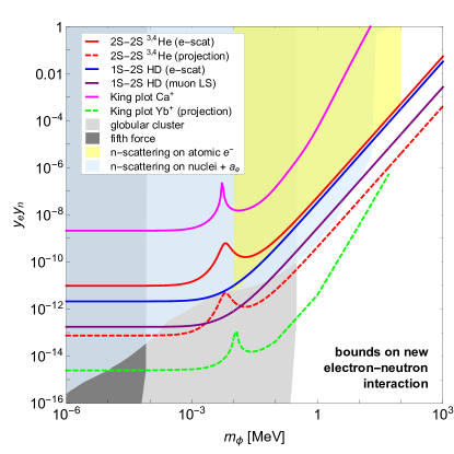
Figure 1: Summary of the indirect constraints on a new electron-neutron interaction: isotope shift spectroscopy of helium and hydrogen/deuterium (this work) with the charge radius determined from electron scattering (“e-scat”) or Lamb shift in muonic atoms (“muon LS”); comparison with King plot analyses of IS in heavy atoms (Ca⁺, Yb⁺) PhysRevLett.115.053003 ; Berengut:2017zuo , fifth force experiments Bordag:2001qi ; bordag2009advances , electron-neutron scattering Adler:1974ge , neutron-nucleus scattering Barbieri:1975xy ; Leeb:1992qf ; Nesvizhevsky:2007by ; Pokotilovski:2006up combined Berengut:2017zuo with $a_{e}$, and globular cluster Hardy:2016kme . The existing bounds are in solid lines, while the projections are in dashed lines. The He projection assumes a combined theory and experimental uncertainty of 100 Hz; the Yb⁺ projection assumes King linearity at 1 Hz.

III.1 Helium and helium-like isotope shifts

We derive here IS bounds using precision spectroscopy in two-electron atoms. This includes constraints from measurements in helium and helium-like lithium and nitrogen ions, all of which are presented in Fig. 2, while the strongest one is also reported in Fig. 1 for comparison with constraints from other atoms and different sources.

The most accurate IS in helium are measured within a few kHz uncertainty between $A=3,4$ for the $2^{1}S-2^{3}S$ Rooij and $2^{3}P-2^{3}S$ Cancio1 ; Cancio2 transitions around $1557\,$nm and $1083\,$nm, respectively. While QED calculations in the point-nucleus limit reached sub-kHz accuracy, the theory prediction for the IS is limited by the charge radius difference $\delta\langle r^{2}\rangle_{3,4}$ Pachucki:2017xcg . The latter can be extracted within a few percent from e-He scattering data Sick:2015spa ,

$$\delta\langle r^{2}\rangle_{3,4}^{\rm e-scat}=(1.067\pm 0.065)\,{\rm fm}^{2}\,.$$ (9)

Using Eq. (9) as an input for the theory predictions of He IS yields a good agreement between theory and experiment for both transitions, thus allowing to constrain NP electron-neutron interactions.

A higher sensitivity could be reached by combining the two transitions in order to eliminate $\delta\langle r^{2}\rangle_{3,4}$. In that case, Eq. (8) results in

$$y_{e}y_{n}\approx\frac{(-51\pm 14)\,{\rm kHz}}{(5.7X_{1557}-X_{1083})}\,,$$ (10)

which is $\sim 4\sigma\,$ away from zero. Thus, it is not justified, given such a disagreement, to use the above to set limits on NP. Note, however, that this large deviation is the mere consequence of a known tension between the two transitions which may originate from underestimated uncertainties Pachucki:2017xcg . Despite this circumstance, it remains interesting to observe that in the case that the tension will be resolved by refined QED calculations and/or measurements, the expected sensitivity to $y_{e}y_{n}$ is stronger by a factor $\sim 6$ relative to the use of $\delta\langle r^{2}\rangle_{3,4}^{\rm e-scat}$. In the (yet implausible) event that the above deviation is an evidence for a new electron-neutron interaction, the latter should be visible in other atomic systems. For instance, Eq. (10) would imply a violation of King linearity in ytterbium ion clock transitions at the $\mathcal{O}(100\,$Hz) level Berengut:2017zuo .

Alternatively, $\delta\langle r^{2}\rangle_{3,4}$ can be extracted with high accuracy from muonic helium spectroscopy. The CREMA collaboration is currently conducting Lamb shift measurements in muonic He⁺ aiming at a determination of ^3,4He charge radii with a relative uncertainty of $3\times 10^{-4}$ Antognini:2011zz . Assuming this will result in a $\delta\langle r^{2}\rangle_{3,4}$ value consistent with e-He scattering and (electronic) helium spectroscopic data, the sensitivity to NP will hence be limited by the experimental accuracy in helium IS measurements. Moreover, future IS measurements in the $2^{1}S-2^{3}S$ transition down to $\mathcal{O}(100\,$Hz) precision are expected VassenTalk:2017 , with a comparable theory improvement. Hence, this would potentially improve sensitivity to NP effects for that transition by two orders of magnitude. As shown in Fig. 1, this is still weaker than the sensitivity expected from King linearity violation in ytterbium ions, except for $m_{\phi}\gtrsim 10\,$MeV due to the different scaling of the bound with the mediator mass ($m_{\phi}^{2}$ versus $m_{\phi}^{3}$).

Precision measurements are also achievable in heavier (unstable) helium isotopes. For instance, IS between $A=4$ and $A=6,8$ isotopes for the $2^{3}S-3^{3}P$ transition ($389\,$nm) are measured with $\sim\!100\,$kHz accuracy Mueller:2008bj . However, the situation is different here since there is no independent measurement of the ^6,8He charge radii and the FS cannot be reliably predicted for the $389\,$nm transition. Nevertheless one can still derive an upper bound on NP by saturating the difference between theory (assuming a point-like nucleus) and experiment, which corresponds to setting $\delta\langle r^{2}\rangle_{AA^{\prime}}=0$ in Eq. (7). Since $\Delta_{389}^{8,4}=-0.918\,$MHz Mueller:2008bj , the NP contribution is not strongly constrained. Yet, the resulting bound on $y_{e}y_{n}$ is strengthened by a factor of $A-A^{\prime}=4$ which makes it comparable to the IS bound from the $1083\,$nm transition. An order of magnitude improvement could be obtained with an independent determination of the charge radii of $A=6,8$ isotope of helium.

Finally, IS in helium-like ions are also well measured. The highest accuracy is obtained in singly-ionized lithium PhysRevA.49.207 and five-times ionized nitrogen PhysRevA.57.180 . The measured frequency shifts are between $A=6,7$ in the $2^{3}S-2^{3}P$ transition for Li⁺, and between $A=14,15$ in the $2^{1}S-2^{3}P$ transition for N⁵⁺. We rely on the theory predictions used in the quoted references. This assumes nuclear charge radii determined from electron-scattering data JagerVries with a relative accuracy of $\sim 2\,\%$ for lithium and from electron-scattering data DEVRIES198822 and muonic X-ray line measurements SCHALLER1980333 with $\sim 0.5\,\%$ for nitrogen. The resulting bounds are weaker than the ones from helium. Further precision measurements with helium-like boron and carbon ions are also underway Pachucki:2017xcg .

isotopes	transition	$\delta_{\rm NP}\nu$	$\sigma_{\nu_{\rm exp}}$	$\sigma_{\nu_{0}}$	$\sigma_{\delta\langle r^{2}\rangle}$
3He/4He	$2^{1}S-2^{3}S$ $2^{3}P-2S$	$+9\pm 14$ $-2\pm 78$	$2.4$ $3.3$	$0.19$ $0.9$	$14$ $78$
H/D	$1S-2S$ $2S-12D$	$+76\pm 61$ $+1.2\pm 10$	0.02 9.3	0.9 4.2	61

Table 1: Allowed NP contributions $\delta_{\rm NP}\nu$ for the most accurate IS measurements in helium and hydrogen isotopes, along with the standard uncertainties from experiment, $\sigma_{\nu_{\rm exp}}$, QED calculation (point-nucleus limit, $\sigma_{\nu_{0}}$) and charge radius difference extracted from electron-scattering data, $\sigma_{\delta\langle r^{2}\rangle}$. Only for $2S-12D$ in H/D, $\sigma_{\nu_{0}}$ refers to the complete theory prediction including the FS. All numbers are in kHz. For references and input values, see Tables 3 and 4.

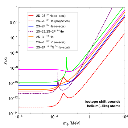
Figure 2: Isotope shift bounds on new electron-neutron interaction from helium spectroscopy. The solid red and blue lines are the limits from the 1557 nm and $1083\,$nm transitions, respectively, using the charge radii from e-He scattering. The dotted-dashed purple line is an illustration of the potential limit obtained by combining the two transitions (due to a $4\sigma$ tension, see text for details). The solid orange line is the upper bound derived from IS in unstable isotopes. The dashed red line represents the projected sensitivity with the 1557 nm transition using charge radii from muonic helium and assuming a combined experimental and theory uncertainty of 100 Hz.

III.2 Hydrogen-deuterium shifts

Hydrogen-deuterium shifts are complementary probes of new electron-neutron interactions. The most accurate IS measurement is for the $1S-2S$ transition ($121.6\,$nm), with $\sim 10^{-11}$ relative uncertainty Parthey:2010aya ; PhysRevA.83.042505 . The QED calculation is less precise by a factor of $\sim 60$, being equally limited by the experimental value of the proton-to-electron and deuteron-to-electron mass ratios as well as higher-order corrections to the Lamb shift and nuclear polarizability Parthey:2010aya . Additional IS measurements exist with lower precision, including the $2S-nS/D$ transition series for $n=8,12$ states deBeauvoir2000 ; PhysRevLett.78.440 ; PhysRevLett.82.4960 , and the frequency differences weitz1995precision

$$\nu_{\rm LS}^{L}\equiv\nu_{2S-4L}-\frac{1}{4}\nu_{1S-2S}\,,$$ (11)

with $L=S,D$. The latter is constructed such that the leading contribution from Coulomb-like potentials cancels out, thus making it directly sensitive to Lamb shift (LS) corrections. As a result, $\nu_{\rm LS}^{L}$ becomes less sensitive to NP with an interaction range longer than the atomic size $\sim a_{0}=(\alpha m_{e})^{-1}\approx(4\,$keV$)^{-1}$. Since all transitions in the $2S-nS/D$ series have comparable sensitivity to NP, we consider only the $2S-12D$ transition for illustration.

Here again, the FS contributions are least known theoretically as they are limited by the charge radius difference $\delta\langle r^{2}\rangle_{2,1}$ between the deuteron and the proton. The latter can be extracted either from electron scattering data, which yields Mohr:2012tt

$$\delta\langle r^{2}\rangle^{\rm e-scat}_{2,1}\!=\!\left(3.764\pm 0.045\right)\,{\rm fm}^{2}\,,$$ (12)

or muonic hydrogen/deuterium spectroscopy Pohl1:2016xoo

$$\delta\langle r^{2}\rangle_{2,1}^{\mu}=\left(3.8112\pm 0.0034\right)\,{\rm fm}^{2}\,.$$ (13)

Note that the charge radius differences in Eqs. (12) and (13) are consistent within uncertainties, despite the (still puzzling) significant discrepancies between muonic and electronic determinations of the proton protonsize2 ; protonsize and deuteron Pohl1:2016xoo radii. Using $\delta\langle r^{2}\rangle_{2,1}^{\mu}$ to predict the FS contribution yields a sensitivity to NP larger by a factor $\sim 13$ relative to $\delta\langle r^{2}\rangle_{2,1}^{\rm e-scat}$, assuming the radii extraction from muonic spectroscopy is not affected by a possible NP coupling to muons.

The IS bounds on a new electron-neutron interaction from hydrogen/deuterium are summarized in Fig. 3.

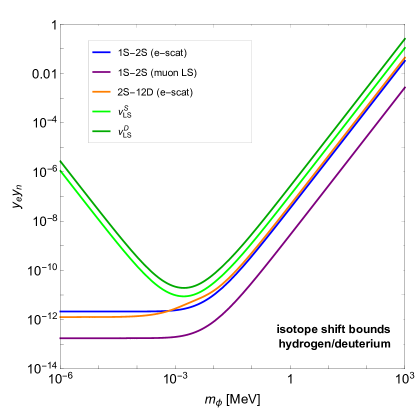
Figure 3: Isotope shift bounds on new electron-neutron interaction from hydrogen/deuterium spectroscopy. The blue (purple) line is the limit from the $1S-2S$ transition using charge radii from electron scattering (muonic spectroscopy). The orange and green lines are limits derived from the $2S-12D$ transition and the $\nu_{\rm LS}^{S,D}$ observables, respectively, using electron-scattering data. See text for details.

IV Bounds from absolute frequency measurements

While IS are only sensitive to electron-neutron interactions, absolute frequencies can also probe the electron-proton and, in atoms with more than one electron or in positronium, electron-electron interactions. As we discussed above, by measuring two transitions one can extract $y_{e}$ and $y_{N}$ separately, and the combination with the IS data will also allow for a separation of $y_{p}$ from $y_{n}$.

In case $\phi$ couples both to protons and neutrons with a similar strength, as in a Higgs portal or gauged $B-L$, the sensitivity to probe NP with IS is expected to be stronger than from the absolute frequency measurements. This can be understood as follows. In light atoms, the NP contributions to the IS and to the absolute frequency are of the same order. However, typically the absolute accuracy of IS data (theory and experiment) is better by at least an order of magnitude than the absolute frequency data, see Appendix A. Thus, for $y_{n}\approx y_{p}$ IS measurements are a more sensitive to NP than the absolute frequencies.

It is important to distinguish between the case of a generic new force coupled to the electron and to the nucleus (including the proton) and the case of a dark photon (kinetic mixing) where the charges are proportional to the electric charges and a more careful treatment of the definition of the electromagnetic coupling, $\alpha$, is required, see Ref. Jaeckel:2010xx .

IV.1 Bounds on $y_{e}$ from helium and positronium

The electron-electron interaction can be probed in atoms with more than one electron, the simplest is helium, or in purely electronic systems such as positronium. Starting with the positronium, the $1^{3}S_{1}-2^{3}S_{1}$ interval is measured at the $10^{-9}$ level Fee:1993zz in a agreement with the theory prediction of Ref. Czarnecki:1999mw . For helium we combine all the transitions that are given in Table II of Ref. Pachucki:2017xcg , where the agreement between theory and experiment is better than $2\sigma$; the full list is given in Appendix A. Thus, we use the above to put upper bounds on $y_{e}$ as function of the force-carrier mass $m_{\phi}\,$. The results are presented in Fig. 4, where we also added the constraint from the electron magnetic moment, $a_{e}$, for comparison. This shows that $a_{e}$ is still the strongest probe among the three. Yet the $\phi$ contribution to $a_{e}$ enters only at the loop level which makes it more prone to cancelation against additional contributions from other states present in a complete NP model. Note that the helium bounds in Fig. 4 are evaluated by assuming no electron-nucleus interactions. We have verified that marginalizing over the latter does not significantly change the bounds. The bounds from positronium and helium are comparable and below few keV are weaker than the bound from $a_{e}$ only a factor of few.

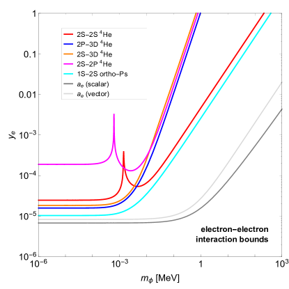
Figure 4: The upper bound on $y_{e}$ as function of $m_{\phi}$ from $1^{3}S_{1}-2^{3}S_{1}$ in positronium Fee:1993zz ; Czarnecki:1999mw  (cyan), helium data Pachucki:2017xcg and a comparison to electron magnetic moment, $a_{e}$, for a scalar (dark gray) and vector (light gray).

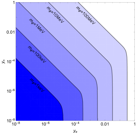
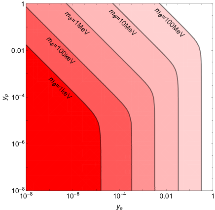
Figure 5: The allowed region 95 % CL contours for fixed mediator mass (as indicated in the plot) from the global $\chi^{2}$ analysis of helium and hydrogen absolute frequencies as well as their isotope shifts. The left (right) panel shows contours of $y_{n}$ ($y_{p}$) vs $y_{e}$, marginalizing over $y_{p}$ ($y_{n}$).

IV.2 Model-independent bounds on $y_{e}$, $y_{p}$ and $y_{e}$

Here we combine observables from different atoms to probe the NP couplings $y_{p}$, $y_{n}$ and $y_{e}$ independently. In order to do so we perform a global fit based on a $\chi^{2}$ function constructed from IS in hydrogen and helium as well as absolute transition frequencies in helium. Our $\chi^{2}$ is composed of the $2^{1}S-2^{3}S$ and $2^{3}P-2S$ IS between ³He and ⁴He, the helium/deuterium IS in the $1S-2S$ transition and the $\nu^{S}_{\rm LS}$ observable, and the absolute frequencies considered in Section IV.1. We present in Fig. 5, the 95 % CL contours in the $y_{e}-y_{p}$ and $y_{e}-y_{n}$ planes for several values of $m_{\phi}$. For each pair of couplings, we marginalize over the third coupling $y_{n}$ and $y_{p}$, respectively. The generic shape of the bounds is understood as follows. Since the overlap integrals $X_{i},Y_{i}$ for electron-nucleus and electron-electron interactions are of comparable order when $y_{p,n}\gtrsim y_{e}$, absolute frequencies and IS constrain the products $y_{e}y_{p}$ and $y_{e}y_{n}$, respectively, leading to contours at 45 degrees. The latter are then truncated once $y_{e}$ reaches a large value (typically $y_{e}\gtrsim y_{p,n}$) so that the $y_{e}^{2}$ term dominates the NP contribution to absolute frequencies in helium and the bounds become independent of $y_{p}$ or $y_{n}$. Note that helium absolute frequencies are in principle sensitive to a possible relative sign between the nuclear and the electron couplings. We checked that either sign yields very similar bounds and thus, for simplicity, we present global-fit results for positive couplings only.

IV.3 Atomic bounds on kinetic mixing

For the sake of illustration, we apply now our result to a specific NP model, that of a kinetically mixed massive gauge boson, the dark photon, denoted as $A^{\prime}$ Holdom:1985ag . As a result of the mixing between the photon and the dark photon, $A^{\prime}$ couples to the electromagnetic current, and its couplings to the protons, electrons and neutrons are $y_{p,n,e}=\epsilon e,0,-\epsilon e$, respectively, where $e$ is the QED gauge coupling constant and $\epsilon$ is a mixing parameter. Since all $A^{\prime}$ couplings are determined by a single parameter, a single atomic transition would suffice to probe it. However, when $m_{A^{\prime}}\lesssim 1/a_{0}$, the dark photon induces a $1/r$ atomic potential which is not distinguishable from the Coulomb one and the $A^{\prime}$ effect is a mere redefinition of the fine-structure constant, $\alpha\to(1+\epsilon^{2})\alpha$. Hence, in this regime, we need at least two observables to probe the dark photon, one of them being used to fix $\alpha$. We follow here the procedure of Ref. Jaeckel:2010xx and combine either two atomic transitions together or one transition with $a_{e}$, the anomalous magnetic moment of the electron. Figure 6 shows the $95\,\%$ CL bounds that we derived from helium and positronium, each combined with $a_{e}$, as well as existing bounds from hydrogen spectroscopy Jaeckel:2010xx ; Karshenboim:2010cg ; Karshenboim:2010ck . We find that helium and positronium bounds surpass the known hydrogen bounds above $\sim 100\,$keV. We chose to present only indirect constraints from atomic spectroscopy on the kinetic-mixing parameter since those do not depend on the $A^{\prime}$ decay mode. In the sub-MeV region, these atomic probes are the most sensitive ones, after the LSND neutrino detector which directly searches for $A^{\prime}$ in the 3 photons decay Pospelov:2017kep , and the study of star cooling in globular clusters which excludes, for $m_{A^{\prime}}\lesssim 300$ keV, mixing parameter values far below the displayed range of $\epsilon$ in Fig. 6. For $m_{A^{\prime}}\gtrsim 1$ MeV, the sensitivity of atomic spectroscopy is also much weaker compared to probes based on $A^{\prime}$ decay (either visibly or invisibly) as in electron beam-dump experiments or colliders, like BaBar (see Ref. Alexander:2016aln for a review). In conclusion, for $m_{A^{\prime}}\gtrsim 0.3$ MeV, the most sensitive indirect probe of dark photon is from combining $a_{e}$ with atomic transitions in helium.

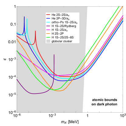
Figure 6: Comparison of atomic (indirect) constraints on the mixing $\epsilon$ between the photon and the dark photon $A^{\prime}$ depending on its mass $m_{A^{\prime}}$. The red/blue (cyan) lines refer to He (positronium) transitions obtained in this work. For comparison, previous bounds from H spectroscopy are shown for $1S-2S$ combined with Rydberg states (purple) or $a_{e}$ (pink) Pospelov:2008zw ; Karshenboim:2010ck ; Karshenboim:2010cg and from one or the combination of two H transitions (orange, green) Jaeckel:2010xx . The range of $m_{A^{\prime}}\leq 300$ keV is excluded by globular clusters Hardy:2016kme ; for $m_{A^{\prime}}\gtrsim 1$ MeV several direct, decay-dependent bounds also apply.

V Discussion

In this work we study the sensitivity to new spin-independent forces of hydrogen and helium-like atoms considering both absolute frequency and isotope shift measurements. We exploit the accuracy of both the measurements and the theoretical predictions achieved in these systems Pachucki:2017xcg ; Karshenboim:2000kv . We demonstrate for the first time the power of isotope shift measurements in few-electrons atoms to constrain models where the new degree of freedom, $\phi$, couples not only to the proton, but also to the neutron as, for instance, in the $B-L$ and Higgs portal models. The derived bounds represent, to date, the strongest laboratory bound on $y_{e}y_{n}$ for $m_{\phi}\gtrsim 100$ eV. For masses heavier than 300 keV, where astrophysical probes are ineffective, isotope shift spectroscopy in few-electron atoms constrains new regions of the parameter space in a model-independent way. Previous works on spin-independent new interactions Jaeckel:2010xx ; Karshenboim:2010cg ; Karshenboim:2010ck focused on hydrogen which is only sensitive to new interactions between the electron and the proton. The highly precise spectroscopy of helium has the advantage to probe also the electron coupling alone, reaching a sensitivity comparable to $a_{e}$ below few keV. (See Ref. Ficek:2016qwp for similar results regarding spin-dependent electron-electron interactions.) Furthermore, we show that current precision in positronium spectroscopy has comparable constraining power.

The present work emphasizes how the effort in improving the knowledge of the nuclear size has the indirect effect of improving the sensitivity to new spin-independent forces between the constituents of the atoms.

Appendix A Experimental Data and Theoretical Prediction

In this appendix we provide all experimental data and theoretical predictions that have been used in this paper.

We start with the nuclear charge radii in Tab. 2 used throughout the paper.

element	$A$	$r_{A}$ [fm]	method	ref.
H/D	1	0.8791 $\pm$ 0.0079	e-scat.	Mohr:2015ccw
	2	2.130 $\pm$ 0.010		Mohr:2015ccw
	1	0.84087 $\pm$ 0.00039	$\mu$-spec.	protonsize ; protonsize2
	2	2.12562 $\pm$ 0.00078		Pohl1:2016xoo
He	3	1.973 $\pm$ 0.016	e-scat.	Sick:2015spa
	4	1.681 $\pm$ 0.004		Sick:2015spa
Li	6	2.589 $\pm$ 0.039	e-scat.	ANGELI201369
	7	2.444 $\pm$ 0.042
N	14	2.560 $\pm$ 0.011	$\mu$-spec.	SCHALLER1980333
	15	2.612 $\pm$ 0.009	e-scat.	DEVRIES198822

Table 2: Charge radii $r_{A}$ used for the IS bounds for different elements with isotopes $A$, obtained via electron-scattering experiments (e-scat.) or spectroscopy in muonic atoms ($\mu$-spec.).

In Tab. 3 we continue with the input values used for the IS bounds in Tab. 1 and Fig. 2 of Sect. III, see also Tab. 5 of Ref. Pachucki:2017xcg . Finally, we provide the values of measurements and calculations of absolute frequencies in Tab. 4.

$A,A^{\prime}$	transition $i$	$\nu_{i}^{AA^{\prime},{\rm exp}}$ [kHz]	ref.	$\nu_{i,0}^{AA^{\prime},{\rm th}}$ [kHz]	$F_{i}$ [kHz/fm2]	ref.
3,4He	$2^{1}S^{1/2}-2^{3}S^{3/2}$	-8 034 286.259$\pm$2.4	drake2006atomic ; PhysRev.187.5 ; PhysRevA.1.571	-8 034 065.91$\pm$0.19	-214.66$\pm$0.02	PhysRevA.94.052508 ; Patkos:2017lnm ; PhysRevA.95.012508 ; 2015JPCRD..44c1206P
	$2^{3}P-2S$	-33 668 444.7$\pm$3.2		-33 667 149.3$\pm$0.9	-1 212.2 $\pm$ 0.1
4,8He	$2S-3P_{2}$	64 701 466$\pm$52	PhysRevLett.99.252501	64 702 409	1 008	PhysRevLett.99.252501
H/D	$1S-2S$	670 994 334.605 $\pm$ 0.015	PhysRevA.83.042505	670 999 566.90$\pm$0.89	-1 369.88	PhysRevA.83.042505
14,15N	$2^{1}S_{0}-2^{3}P_{1}$	649 418 424.16$\pm$29 979.2	PhysRevA.57.180	649 469 388.8 $\pm$ 269 812.8		PhysRevA.57.180
6,7Li	$2^{3}P_{0}-2^{3}S_{1}$	3 474 773$\pm$55	PhysRevA.49.207	34 747 876		PhysRevA.49.207

Table 3: Theoretical and experimental input values for the IS bounds: measured IS $\nu_{i}^{AA^{\prime},{\rm exp}}$, theory prediction for a point-like nucleus $\nu_{i,0}^{AA^{\prime},{\rm th}}$, and the field shift constant $F_{i}$. See also Ref. Pachucki:2017xcg . For the IS of $2S-12D$ in H/D, see the absolute frequencies in Tab. 4. $F_{1S-2S}$ for H/D is an approximate value obtained from the quoted FS in Ref. PhysRevA.83.042505 .

element	transition $i$	$\nu_{i}^{\rm exp}$ [kHz]	ref.	$\nu_{i}^{\rm th}$ [kHz]	ref
H	$2S_{1/2}-12D_{3/2,5/2}$	799 191 727 402.8 $\pm$ 6.7	deBeauvoir2000	799 191 727 409.1 $\pm$ 3.0	PhysRevLett.95.163003
D		799 409 184 967.6 $\pm$ 6.5	deBeauvoir2000	799 409 184 973.4 $\pm$ 3.0
H	$(4S_{1/2}-2S_{1/2})-\frac{1}{4}(2S-1S)$	4797338 $\pm$ 10	weitz1995precision	4 797 329 $\pm$ 5	weitz1995precision
D		4 801 693 $\pm$ 20		4 801 692 $\pm$ 5
H	$(4S_{1/2}-2D_{5/2})-\frac{1}{4}(2S-1S)$	6 490 144 $\pm$24		6 490 128 $\pm$ 5
D		6 494 841 $\pm$ 41		6 494 816 $\pm$ 5
4He	$2^{1}S_{0}-2^{3}S_{1}$	192 510 702 145.6 $\pm$ 1.8	Pachucki:2017xcg	192 510 703 400 $\pm$ 800	Pachucki:2017xcg
	$2^{3}P_{0}-3^{3}D_{1}$	510 059 755 352 $\pm$ 28		510 059 754 000 $\pm$ 700
	$2^{3}S_{1}-3^{3}D_{1}$	786 823 850 002 $\pm$ 56		786 823 848 400 $\pm$ 1 300
	$2^{1}S_{0}-2^{1}P_{1}$	145 622 892 886 $\pm$ 183		145 622 891 500 $\pm$ 2 300
Ps	$1^{3}S_{1}-2^{3}S_{1}$	1 233 607 216 400 $\pm$ 3200	Fee:1993zz	1 233 607 222 180 $\pm$ 580	Czarnecki:1999mw

Table 4: Measurements and predictions of absolute transition frequencies in H, D, He and positronium (Ps). The H and D values are used for the H/D IS in Sect. III.2. The middle part of the table summarizes the experimental and theoretical frequencies of the Lamb shift $(4L-2S_{1/2})-\frac{1}{4}(2S-1S)$ for $L=S,D$. The lower part of the table is used for constraining $y_{e}$ in Fig. 4: the transitions in ⁴He with an agreement of better than $2\sigma$ between theory and experiment, as well as a transition in Ps.

Appendix B Helium wavefunction

In this appendix we specify the approximate wavefunctions we use in the helium calculations. It is conventional to label the states of helium as

$$n^{2S+1}L_{J}$$ (14)

corresponding to the following electronic configuration $(1s)(nl)$. $L$ is the total orbital momentum, $S$ is the spin and $J\leq L+S$ is the total angular momentum. Since one electron is always in the $(1s)$ orbital $L=l$, and $S=0,1$ corresponding to the singlet and triplet states, respectively.

For two-electron systems in the non-relativistic limit, the spin and spatial parts of the wavefunction are factorized. The spin singlet ($S=0$) state is

$$|S=0,m_{S}=0\rangle=\frac{|\uparrow\downarrow\rangle-|\downarrow\uparrow\rangle}{\sqrt{2}}\,,$$ (15)

while the spin triplet ($S=1$) is with components

$$|S=1,m_{S}=1\rangle=|\uparrow\uparrow\rangle\,,$$

$$|S=1,m_{S}=0\rangle=\frac{|\uparrow\downarrow\rangle+|\downarrow\uparrow\rangle}{\sqrt{2}}\,,$$

$$|S=1,m_{S}=-1\rangle=|\downarrow\downarrow\rangle\,.$$ (16)

Using an antisymmetrized combination of hydrogenic orbitals, the spatial part of the wavefunction takes the form

$$\langle\vec{r}_{1},\vec{r}_{2}|\psi_{nlm}^{S}\rangle=\frac{1}{2\sqrt{\pi}}\frac{1}{\sqrt{2(1+N_{nl})}}\times$$

$$\left[F_{nl}(r_{1},r_{2})Y_{lm}(\Omega_{2})+(-1)^{S}F_{nl}(r_{2},r_{1})Y_{lm}(\Omega_{1})\right]\,,$$ (17)

where the $1/(2\sqrt{\pi})$ prefactor is the $Y_{00}$ spherical harmonic from the $1s$ electron, and $N_{nl}$ ensures that the radial part of the wavefunction is canonically normalized. We write the $F_{nl}$’s as products of non-relativistic hydrogen radial wavefunctions as

$$F_{nl}(r_{1},r_{2})=R_{10}(r_{1},Z_{i})R_{nl}(r_{2},Z_{a})\,,$$ (18)

where (in units of $a_{0}=1$)

$$R_{nl}(r,Z)\!=\!\left(\frac{2Z}{n}\right)^{3/2}\!\!\!\!\sqrt{\frac{(n-l-1)!}{2n(n+l)!}}e^{-\rho/2}\rho^{l}L_{n-l-1}^{2l+1}(\rho)\,,$$ (19)

where $\rho=2rZ/n$, $L_{k}^{\alpha}(x)$ are the generalized Laguerre polynomials of degree $k$, and $Z_{i}$ and $Z_{a}$ are the effective nuclear charges for the core $(1s)$ and valence $(nl)$ electrons, respectively. An important point is that $Z_{i,a}\neq Z=2$ because of screening effects; they depend on the electronic configuration considered, see Table 5. The $R_{nl}$’s form an orthonormal basis for a fixed $Z$. However, because the two electrons effectively feel a different nuclear charge ($Z_{i}\neq Z_{a}$), there is an overall normalization constant for $S$ waves because of the cross term in the square of Eq. (B)

$$N_{nl}=(-1)^{S}\delta_{l,0}\left[\int drr^{2}R_{10}(r,Z_{i})R_{nl}(r,Z_{a})\right]^{2}\,,$$ (20)

which vanishes for $Z_{i}=Z_{a}$ and $n\geq 2$ by orthogonality of $R_{nl}(r,Z)$.

state	$Z_{i}$	$Z_{a}$
$(2)^{1}S$	$2.08$	$1.21$
$(2)^{3}S$	$2.01$	$1.53$
$(2)^{3}P$	$2.00$	$0.97$
$(2)^{3}P$	$1.99$	$1.09$
$n\geq 3$	$2$	$1$

Table 5: Effective nuclear charges for the excited states of helium under consideration. $Z_{i}$ is the charge of the core (1s) electron and $Z_{a}$ is the charge of the excited electron. These are obtained by variational methods using the non-relativistic hydrogen wavefunctions as trial functions. When the electron is excited to a $n=3$ or higher orbital, the screening of the core electron is found nearly perfect.

The total wavefunction for a fixed $J$ and (its projection) $m_{J}=-J\dots J$ are then constructed from $L\times S$ combination of angular momentum using the Clebsch-Gordan coefficients $C_{L,m,S,m_{S}}^{J,m_{J}}$ as

$$|n^{2S+1}L_{J,m_{J}}\rangle=\sum_{m=-L}^{L}\sum_{m_{S}=-S}^{S}C_{L,m,S,m_{S}}^{J,m_{J}}|\psi_{nLm}\rangle|S,m_{S}\rangle.$$ (21)

We use the above wavefunctions for all helium states with the exceptions of the $2^{1}S$, $2^{3}S$ and $2^{3}P$ states where we use non-relativistic wavefunctions based on Hylleraas functions taken from Refs. 1948ApJ…108..354H ; PhysRev.116.914 in order to better describe the repulsion between the two electrons. This turns out to be of particular importance for the $2^{1}S$ state. Indeed, for spin-singlet states, the spatial part of the wavefunction is symmetric under the exchange of the two-electrons so that the wavefunction in Eq. (B) may over-estimate the electronic density is in the region where the electrons are close to each other, $r_{1}\sim r_{2}$. Hylleraas functions then provide a more accurate description of the electron repulsion effect by introducing an explicit dependence on the inter-electronic distance $r_{12}$ in the wavefunction. The spatial part of wavefunction is then taken to be of the form

$$\langle\vec{r}_{1},\vec{r}_{2}|\psi_{nlm}^{S}\rangle=\frac{1}{\sqrt{N}}\left[F_{nl}(r_{1},r_{2},r_{12})Y_{lm}(\Omega_{2})+\right.$$

$$\left.+(-1)^{S}F_{nl}(r_{2},r_{1},r_{12})Y_{lm}(\Omega_{1})\right]$$ (22)

where $N$ is a normalization constant and $F_{nl}$ now depends on $r_{12}$ and is expanded on Hylleraas functions as

$$F_{nl}(r_{1},r_{2},r_{12}) = [\kappa(s+t)]^{l}e^{-\frac{\kappa}{2}\left(s-\sigma t\right)}$$ (23)

$$\times\sum_{i=1}^{k}c_{i}\phi_{i}(\kappa s,-\kappa t,\kappa u)\,,$$

with $s\equiv r_{1}+r_{2}$, $t\equiv r_{2}-r_{1}$, $u\equiv r_{12}$ and $\phi_{i}(s,t,u)=s^{p_{i}}t^{q_{i}}u^{r_{i}}$. It is convenient to reorganize the Hylleraas terms according to their powers of $r_{12}$. We then write the radial function in Eq. (23) as

$$F_{nl}(r_{1},r_{2},r_{12})=\sum_{i=0}^{k}f_{i}(r_{1},r_{2})r_{12}^{i}\,.$$ (24)

Appendix C Overlap integrals for helium

In this appendix we give the analytical expressions for the overlap integrals for the case of helium, i.e.  the electronic NP coefficients $X_{i}$ and $Y_{i}$.

C.1 Electron-nucleus interactions

Let us consider the potential of Eq. (1) between the nucleus and its bound electron with the above helium wavefunctions. In first-order perturbation theory we find

$$X_{i}\equiv \hat{X}_{a}-\hat{X}_{b}$$

$$= \frac{1}{4\pi}\int\left[\prod_{k=1}^{n_{e}}d^{3}r_{i}\right]\,\left[\sum_{i=1}^{n_{e}}\frac{e^{-m_{\phi}r_{i}}}{r_{i}}\right]$$

$$\times\left[|\Psi_{a}(\vec{r}_{1},\dots,\vec{r}_{n_{e}})|^{2}-|\Psi_{b}(\vec{r}_{1},\dots,\vec{r}_{n_{e}})|^{2}\right]\,,$$ (25)

where $n_{e}$ is the number of bound electrons and $|\Psi|^{2}$ is the electron wavefunction density. Using hydrogenic wavefunctions in Eq. (B) the contributions from each state is

$$\hat{X}_{n^{2S+1}L_{J,m_{J}}}= -\frac{1}{4\pi(1+N_{nL})}\left[\int drre^{-m_{\phi}r}\left[R_{10}(r,Z_{i})^{2}+R_{nL}(r,Z_{a})^{2}\right]\right.$$

$$+2(-1)^{S}\delta_{L,0}\int drre^{-m_{\phi}r}R_{10}(r,Z_{i})R_{nL}(r,Z_{a})\left.\times\int drr^{2}R_{10}(r,Z_{i})R_{nL}(r,Z_{a})\right]\,.$$ (26)

For the case of Hylleraas wavefunctions in Eq. (B), we need the following expansion of $r_{12}$ raised to the power $k$ on spherical harmonics

$$r_{12}^{k}=4\pi\sum_{l=0}^{\infty}H^{(k)}_{l}(r_{1},r_{2})\sum_{m=-l}^{l}Y_{lm}(\Omega_{1})Y_{lm}^{*}(\Omega_{2}),$$ (27)

where the coeffcients can be written in closed form in terms of hypergeometric functions sack1964generalization

$$H_{l}^{(n)}(r_{1},r_{2})=\frac{(-n/2)_{l}}{(1/2)_{l}}\frac{r_{>}^{n}}{2l+1}\left(\frac{r_{<}}{r_{>}}\right)^{l}$$

$$\times F\left[l-n/2,-(n+1)/2;l+3/2;\frac{r_{<}^{2}}{r_{>}^{2}}\right]\,,$$ (28)

with $F(\alpha,\beta;\gamma;x)$ denoting the Gauss hypergeometric function and $(\xi)_{s}\equiv\Gamma(\xi+s)/\Gamma(\xi)$. We then find

$$\hat{X}_{n^{2S+1}L_{J,m_{J}}}= -\frac{1}{4\pi N}\int r_{1}^{2}r_{2}^{2}dr_{1}dr_{2}\left(\frac{e^{-m_{\phi}r_{1}}}{r_{1}}+\frac{e^{-m_{\phi}r_{2}}}{r_{2}}\right)$$

$$\times\int d\Omega_{1}d\Omega_{2}|\psi_{nlm}^{S}|^{2}\,,$$ (29)

where the square of the spatial wavefunction integrated over the angular variables is

$$\int d\Omega_{1}d\Omega_{2}|\psi_{nlm}^{S}|^{2}= f_{0}(r_{1},r_{2})^{2}+\sum_{i+j\geq 1}H^{(i+j)}_{0}(r_{1},r_{2})f_{i}(r_{1},r_{2})f_{j}(r_{1},r_{2})+[r_{1}\leftrightarrow r_{2}]$$

$$+2(-1)^{S}\left[f_{0}(r_{1},r_{2})f_{0}(r_{2},r_{1})\delta_{l0}+\sum_{i+j\geq 1}H_{l}^{(i+j)}(r_{1},r_{2})f_{i}(r_{1},r_{2})f_{j}(r_{2},r_{1})\right]\,.$$ (30)

C.2 Electron-electron interactions

Consider the NP potential between the bounded electrons, $V_{e}(r_{12})$ see Eq. (1). It is useful to expand the Yukawa potential over spherical harmonics as, see for example 0953-4075-45-23-235003 ,

$$\frac{e^{-mr_{12}}}{r_{12}}\!=\!4\pi\sum_{l=0}^{\infty}G_{l}(r_{1},r_{2},m)\!\!\!\sum_{m=-l}^{l}\!\!\!Y_{lm}(\Omega_{1})Y^{*}_{lm}(\Omega_{2})\,,$$ (31)

where the coefficients are

$$G_{l}(r_{1},r_{2},m)=\frac{I_{l+1/2}(mr_{<})}{\sqrt{r_{<}}}\frac{K_{l+1/2}(mr_{>})}{\sqrt{r_{>}}}\,,$$ (32)

with $I$ and $K$ the modified Bessel functions of the first and second kind respectively and $r_{>}$ ($r_{<}$) is the greater (lesser) of $r_{1}$ and $r_{2}$. For Hylleraas wavefunctions which involve additional powers of $r_{12}$ it will be convenient to use Eq. (31) as a “generating functional” in order to derive the expansion of any $r_{12}^{k-1}e^{-mr_{12}}$ functions (for $k\geq 1$) by differentiating $k-$times the coefficients $G_{l}(r_{1},r_{2},m)$.

The first-order perturbation theory result is

$$Y_{i}\equiv \hat{Y}_{a}-\hat{Y}_{b}$$

$$= \frac{1}{4\pi}\int\left[\prod_{k=1}^{n_{e}}d^{3}r_{i}\right]\,\left[\sum_{i>j}^{n_{e}}\frac{e^{-m_{\phi}r_{ij}}}{r_{ij}}\right]$$

$$\times\left[|\Psi_{a}(\vec{r_{1}},\dots,\vec{r_{n_{e}}})|^{2}-|\Psi_{b}(\vec{r_{1}},\dots,\vec{r_{n_{e}}})|^{2}\right]\,.$$ (33)

Using the expansion of Eq. (31) and the hydrogenic wavefunctions from Eq. (B) we find

$$\hat{Y}_{n^{2S+1}L_{J,m_{J}}}=-\frac{1}{4\pi(1+N_{nL})}\int dr_{1}dr_{2}r_{1}^{2}r_{2}^{2}\big{[} G_{0}(r_{1},r_{2})R_{10}(r_{1},Z_{i})^{2}R_{nL}(r_{2},Z_{a})^{2}$$

$$+(-1)^{S}G_{L}(r_{1},r_{2})R_{10}(r_{1},Z_{i})R_{10}(r_{2},Z_{i})R_{nL}(r_{1},Z_{a})R_{nL}(r_{2},Z_{a})\big{]}\,.$$ (34)

where only $G_{0,L}$ coefficients in the Yukawa expansion of Eq. (31) are needed. Note that the integrand above no longer depends on $m^{\prime}$ and $m_{S}$ hence the sum over Clebsch-Gordan coeffecients squared gives $\sum_{m^{\prime},m_{S}}[C_{L,m^{\prime},S,m_{S}}^{J,m_{J}}]^{2}=1$ by orthonormality. Finally, note that the shift in Eq. (C.2) is indepedent of $J$ and $m_{J}$, which is expected since the potential in Eq. (1) is invariant under rotations. We also used the fact the $G_{l}(r_{1},r_{2})=G_{l}(r_{2},r_{1})$ to simplify the expression.

For the case of Hylleraas wavefunctions in Eq. (B), we find

$$\hat{Y}_{n^{2S+1}L_{J,m_{J}}}= -\frac{1}{4\pi N}\int r_{1}^{2}r_{2}^{2}dr_{1}dr_{2}$$

$$\times\int d\Omega_{1}d\Omega_{2}\frac{e^{-mr_{12}}}{r_{12}}|\psi_{nlm}^{S}|^{2}\,,$$ (35)

where the angular integral simplifies to

$$\int d\Omega_{1}d\Omega_{2}\frac{e^{-mr_{12}}}{r_{12}}|\psi_{nlm}^{S}|^{2}= \sum_{ij}G^{(i+j)}_{0}(r_{1},r_{2})\left[f_{i}(r_{1},r_{2})f_{j}(r_{1},r_{2})+f_{i}(r_{2},r_{1})f_{j}(r_{2},r_{1})\right]$$

$$+2(-1)^{S}\sum_{ij}G_{l}^{(i+j)}(r_{1},r_{2})f_{i}(r_{1},r_{2})f_{j}(r_{2},r_{1})\,,$$ (36)

where ^(k) indicates the $k$th differentiation with respect to $m$,

$$G_{l}^{(k)}(r_{1},r_{2},m)\equiv(-1)^{k}\frac{\partial^{k}G_{l}(r_{1},r_{2},m)}{\partial m^{k}}\,.$$ (37)

In Fig. 7 we evaluate the impact of the Hylleraas wavefunctions on the electronic NP constants by calculating the ratios to the respective quantity based on hydrogen-like wavefunctions, $X_{i}^{\rm Hylleraas}/X_{i}^{\rm H-like}$, $Y_{i}^{\rm Hylleraas}/Y_{i}^{\rm H-like}$.

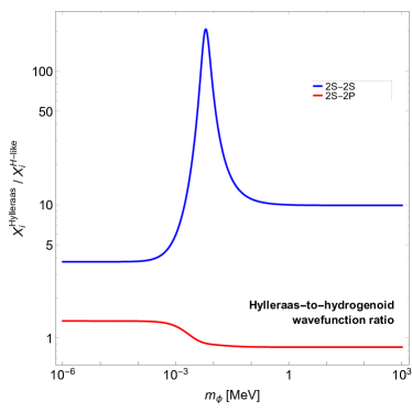
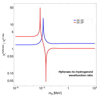
Figure 7: Comparison of the electronic NP coefficients $X_{i},~{}\,Y_{i}$ based on hydrogen-like and Hylleraas wavefunctions depending on the mediator mass $m_{\phi}$ for the transitions $2S-2S$ and $2P-2S$ in helium.

References

- (1) S. G. Porsev, K. Beloy, and A. Derevianko, “Precision determination of electroweak coupling from atomic parity violation and implications for particle physics,” Phys. Rev. Lett. 102 (2009) 181601.
- (2) K. Tsigutkin, D. Dounas-Frazer, A. Family, J. E. Stalnaker, V. V. Yashchuk, and D. Budker, “Observation of a Large Atomic Parity Violation Effect in Ytterbium,” Phys. Rev. Lett. 103 (2009) 071601.
- (3) K. Tsigutkin, D. Dounas-Frazer, A. Family, J. E. Stalnaker, V. V. Yashchuk, and D. Budker, “Parity violation in atomic ytterbium: Experimental sensitivity and systematics,” Phys. Rev. A81 (Mar, 2010) 032114.
- (4) N. Leefer, L. Bougas, D. Antypas, and D. Budker, “Towards a new measurement of parity violation in dysprosium,” 2014. arXiv:1412.1245 [physics.atom-ph].
- (5) O. O. Versolato et al., “Atomic parity violation in a single trapped radium ion,” Hyperfine Interact. 199 no. 1-3, (2011) 9–19.
- (6) V. A. Dzuba, J. C. Berengut, V. V. Flambaum, and B. Roberts, “Revisiting parity non-conservation in cesium,” Phys. Rev. Lett. 109 (2012) 203003, arXiv:1207.5864 [hep-ph].
- (7) B. M. Roberts, V. A. Dzuba, and V. V. Flambaum, “Parity and Time-Reversal Violation in Atomic Systems,” Ann. Rev. Nucl. Part. Sci. 65 (2015) 63–86, arXiv:1412.6644 [physics.atom-ph].
- (8) K. P. Jungmann, “Symmetries and fundamental interactions-selected topics,” Hyperfine Interact. 227 (2014) 5–16.
- (9) Particle Data Group Collaboration, K. A. Olive et al., “Review of Particle Physics,” Chin. Phys. C38 (2014) 090001.
- (10) R. M. Godun, P. B. R. Nisbet-Jones, J. M. Jones, S. A. King, L. A. M. Johnson, H. S. Margolis, K. Szymaniec, S. N. Lea, K. Bongs, and P. Gill, “Frequency Ratio of Two Optical Clock Transitions in and Constraints on the Time Variation of Fundamental Constants,” Phys. Rev. Lett. 113 (Nov, 2014) 210801.
- (11) N. Huntemann, M. Okhapkin, B. Lipphardt, S. Weyers, C. Tamm, and E. Peik, “High-Accuracy Optical Clock Based on the Octupole Transition in ,” Phys. Rev. Lett. 108 (Feb, 2012) 090801.
- (12) J. Reichert, M. Niering, R. Holzwarth, M. Weitz, T. Udem, and T. W. Hänsch, “Phase Coherent Vacuum-Ultraviolet to Radio Frequency Comparison with a Mode-Locked Laser,” Phys. Rev. Lett. 84 (Apr, 2000) 3232–3235.
- (13) J. Reichert, R. Holzwarth, T. Udem, and T. Hänsch, “Measuring the frequency of light with mode-locked lasers,” Optics Communications 172 no. 1, (1999) 59 – 68.
- (14) N. Huntemann, C. Sanner, B. Lipphardt, C. Tamm, and E. Peik, “Single-Ion Atomic Clock with Systematic Uncertainty,” Phys. Rev. Lett. 116 (Feb, 2016) 063001.
- (15) B. J. Bloom, T. L. Nicholson, J. R. Williams, S. L. Campbell, M. Bishof, X. Zhang, W. Zhang, S. L. Bromley, and J. Ye, “An Optical Lattice Clock with Accuracy and Stability at the Level,” Nature 506 (2014) 71–75, arXiv:1309.1137 [physics.atom-ph].
- (16) C. Delaunay, R. Ozeri, G. Perez, and Y. Soreq, “Probing The Atomic Higgs Force,” arXiv:1601.05087 [hep-ph].
- (17) C. Frugiuele, E. Fuchs, G. Perez, and M. Schlaffer, “Constraining New Physics Models with Isotope Shift Spectroscopy,” Phys. Rev. D96 no. 1, (2017) 015011, arXiv:1602.04822 [hep-ph].
- (18) C. Delaunay and Y. Soreq, “Probing New Physics with Isotope Shift Spectroscopy,” arXiv:1602.04838 [hep-ph].
- (19) J. C. Berengut et al., “Probing new light force-mediators by isotope shift spectroscopy,” arXiv:1704.05068 [hep-ph].
- (20) W. H. King, “Comments on the Article “Peculiarities of the Isotope Shift in the Samarium Spectrum”,” J. Opt. Soc. Am. 53 no. 5, (May, 1963) 638–639.
- (21) K. Pachucki, V. Patkóš, and V. Yerokhin, “Testing fundamental interactions on the helium atom,” Phys. Rev. A95 no. 6, (2017) 062510, arXiv:1704.06902 [physics.atom-ph].
- (22) S. G. Karshenboim, “Precise physics of simple atoms,” AIP Conf. Proc. 551 (2001) 238–253, arXiv:hep-ph/0007278 [hep-ph].
- (23) S. G. Karshenboim, “Constraints on a long-range spin-independent interaction from precision atomic physics,” Phys. Rev. D82 (2010) 073003, arXiv:1005.4872 [hep-ph].
- (24) S. G. Karshenboim, “Precision physics of simple atoms and constraints on a light boson with ultraweak coupling,” Phys. Rev. Lett. 104 (2010) 220406, arXiv:1005.4859 [hep-ph].
- (25) J. Jaeckel and S. Roy, “Spectroscopy as a test of Coulomb’s law: A Probe of the hidden sector,” Phys. Rev. D82 (2010) 125020, arXiv:1008.3536 [hep-ph].
- (26) F. Ficek, D. F. J. Kimball, M. Kozlov, N. Leefer, S. Pustelny, and D. Budker, “Constraints on exotic spin-dependent interactions between electrons from helium fine-structure spectroscopy,” Phys. Rev. A95 no. 3, (2017) 032505, arXiv:1608.05779 [physics.atom-ph].
- (27) C. Eckart, “The Theory and Calculation of Screening Constants,” Phys. Rev. 36 (Sep, 1930) 878–892.
- (28) E. A. Hylleraas, “Über den Grundzustand des Heliumatoms,” Zeitschrift für Physik 48 no. 7, (Jul, 1928) 469–494.
- (29) E. A. Hylleraas, “Neue Berechnung der Energie des Heliums im Grundzustande, sowie des tiefsten Terms von Ortho-Helium,” Zeitschrift für Physik 54 no. 5, (May, 1929) 347–366.
- (30) K. Pachucki and V. A. Yerokhin, “Theory of the Helium Isotope Shift,” Journal of Physical and Chemical Reference Data 44 no. 3, (2015) 031206, arXiv:1503.07727 [physics.atom-ph].
- (31) Y.-S. Liu, D. McKeen, and G. A. Miller, “Electrophobic Scalar Boson and Muonic Puzzles,” Phys. Rev. Lett. 117 no. 10, (2016) 101801, arXiv:1605.04612 [hep-ph].
- (32) D. Tucker-Smith and I. Yavin, “Muonic hydrogen and MeV forces,” Phys. Rev. D83 (2011) 101702, arXiv:1011.4922 [hep-ph].
- (33) I. Beltrami et al., “New Precision Measurements of the Muonic 3- (5/2) - 2p (3/2) X-ray Transition in 24Mg and 28Si: Vacuum Polarization Test and Search for Muon - Hadron Interactions Beyond QED,” Nucl. Phys. A451 (1986) 679–700.
- (34) R. Pohl et al., “The size of the proton,” Nature 466 (2010) 213–216.
- (35) A. Antognini et al., “Proton Structure from the Measurement of Transition Frequencies of Muonic Hydrogen,” Science 339 (2013) 417–420.
- (36) CREMA Collaboration, R. Pohl et al., “Laser spectroscopy of muonic deuterium,” Science 353 no. 6300, (2016) 669–673.
- (37) Particle Data Group Collaboration, C. Patrignani et al., “Review of Particle Physics,” Chin. Phys. C40 no. 10, (2016) 100001.
- (38) D. Hanneke, S. F. Hoogerheide, and G. Gabrielse, “Cavity Control of a Single-Electron Quantum Cyclotron: Measuring the Electron Magnetic Moment,” Phys. Rev. A83 (2011) 052122, arXiv:1009.4831 [physics.atom-ph].
- (39) S. L. Adler, R. F. Dashen, and S. B. Treiman, “Comments on Proposed Explanations for the mu - Mesic Atom x-Ray Discrepancy,” Phys. Rev. D10 (1974) 3728.
- (40) R. Barbieri and T. E. O. Ericson, “Evidence Against the Existence of a Low Mass Scalar Boson from Neutron-Nucleus Scattering,” Phys. Lett. 57B (1975) 270–272.
- (41) H. Leeb and J. Schmiedmayer, “Constraint on hypothetical light interacting bosons from low-energy neutron experiments,” Phys. Rev. Lett. 68 (1992) 1472–1475.
- (42) V. V. Nesvizhevsky, G. Pignol, and K. V. Protasov, “Neutron scattering and extra short range interactions,” Phys. Rev. D77 (2008) 034020, arXiv:0711.2298 [hep-ph].
- (43) Yu. N. Pokotilovski, “Constraints on new interactions from neutron scattering experiments,” Phys. Atom. Nucl. 69 (2006) 924–931, arXiv:hep-ph/0601157 [hep-ph].
- (44) M. Bordag, U. Mohideen, and V. M. Mostepanenko, “New developments in the Casimir effect,” Phys. Rept. 353 (2001) 1–205, arXiv:quant-ph/0106045 [quant-ph].
- (45) M. Bordag, G. L. Klimchitskaya, U. Mohideen, and V. M. Mostepanenko, “Advances in the Casimir effect,” Int. Ser. Monogr. Phys. 145 (2009) 1–768.
- (46) G. Raffelt, “Limits on a CP-violating scalar axion-nucleon interaction,” Phys. Rev. D86 (2012) 015001, arXiv:1205.1776 [hep-ph].
- (47) Particle Data Group Collaboration, W. M. Yao et al., “Review of Particle Physics,” J. Phys. G33 (2006) 1–1232.
- (48) J. A. Grifols and E. Masso, “Constraints on Finite Range Baryonic and Leptonic Forces From Stellar Evolution,” Phys. Lett. B173 (1986) 237–240.
- (49) J. A. Grifols, E. Masso, and S. Peris, “Energy Loss From the Sun and RED Giants: Bounds on Short Range Baryonic and Leptonic Forces,” Mod. Phys. Lett. A4 (1989) 311.
- (50) E. Hardy and R. Lasenby, “Stellar cooling bounds on new light particles: plasma mixing effects,” JHEP 02 (2017) 033, arXiv:1611.05852 [hep-ph].
- (51) J. Redondo and G. Raffelt, “Solar constraints on hidden photons re-visited,” JCAP 1308 (2013) 034, arXiv:1305.2920 [hep-ph].
- (52) E. J. Salumbides, W. Ubachs, and V. I. Korobov, “Bounds on fifth forces at the sub-Angstrom length scale,” J. Molec. Spectrosc. 300 (2014) 65, arXiv:1308.1711 [hep-ph].
- (53) W. Ubachs, J. C. J. Koelemeij, K. S. E. Eikema, and E. J. Salumbides, “Physics beyond the Standard Model from hydrogen spectroscopy,” arXiv:1511.00985 [physics.atom-ph].
- (54) J. Biesheuvel, J.-P. Karr, L. Hilico, K. S. E. Eikema, W. Ubachs, and J. C. J. Koelemeij, “High-precision spectroscopy of the HD+ molecule at the 1-p.p.b. level,” Applied Physics B 123 no. 1, (Dec, 2016) 23.
- (55) “Physics beyond the Standard Model from hydrogen spectroscopy,” Journal of Molecular Spectroscopy 320 (2016) 1 – 12.
- (56) B. Feldman and A. E. Nelson, “New regions for a chameleon to hide,” JHEP 08 (2006) 002, arXiv:hep-ph/0603057 [hep-ph].
- (57) A. E. Nelson and J. Walsh, “Chameleon vector bosons,” Phys. Rev. D77 (2008) 095006, arXiv:0802.0762 [hep-ph].
- (58) C. Burrage, “Supernova Brightening from Chameleon-Photon Mixing,” Phys. Rev. D77 (2008) 043009, arXiv:0711.2966 [astro-ph].
- (59) C. Burrage and J. Sakstein, “A Compendium of Chameleon Constraints,” JCAP 1611 no. 11, (2016) 045, arXiv:1609.01192 [astro-ph.CO].
- (60) P. Brax and C. Burrage, “Atomic Precision Tests and Light Scalar Couplings,” Phys. Rev. D83 (2011) 035020, arXiv:1010.5108 [hep-ph].
- (61) J. Alexander et al., “Dark Sectors 2016 Workshop: Community Report,” 2016. arXiv:1608.08632 [hep-ph].
- (62) F. Gebert, Y. Wan, F. Wolf, C. N. Angstmann, J. C. Berengut, and P. O. Schmidt, “Precision Isotope Shift Measurements in Calcium Ions Using Quantum Logic Detection Schemes,” Phys. Rev. Lett. 115 (2015) 053003.
- (63) R. van Rooij, J. S. Borbely, J. Simonet, M. D. Hoogerland, K. S. E. Eikema, R. A. Rozendaal, and W. Vassen, “Frequency Metrology in Quantum Degenerate Helium: Direct Measurement of the 2 3S1 → 2 1S0 Transition,” Science 333 no. 6039, (2011) 196–198.
- (64) P. Cancio Pastor, L. Consolino, G. Giusfredi, P. De Natale, M. Inguscio, V. A. Yerokhin, and K. Pachucki, “Frequency Metrology of Helium around 1083 nm and Determination of the Nuclear Charge Radius,” Phys. Rev. Lett. 108 (Apr, 2012) 143001.
- (65) P. C. Pastor, G. Giusfredi, P. D. Natale, G. Hagel, C. de Mauro, and M. Inguscio, “Absolute Frequency Measurements of the Atomic Helium Transitions around 1083 nm,” Phys. Rev. Lett. 92 (Jan, 2004) 023001.
- (66) I. Sick, “Form factors and radii of light nuclei,” arXiv:1505.06924 [nucl-ex].
- (67) A. Antognini et al., “Illuminating the proton radius conundrum: The mu He+ Lamb shift,” Can. J. Phys. 89 no. 1, (2011) 47–57.
- (68) W. Vassen, “Ultracold He spectroscopy: QED test, line shapes and nuclear sizes.” Talk at FKK 2017, Warsaw.
- (69) P. Mueller et al., “Nuclear charge radius of He-8,” Phys. Rev. Lett. 99 (2007) 252501, arXiv:0801.0601 [nucl-ex].
- (70) E. Riis, A. G. Sinclair, O. Poulsen, G. W. F. Drake, W. R. C. Rowley, and A. P. Levick, “Lamb shifts and hyperfine structure in and : Theory and experiment,” Phys. Rev. A 49 (Jan, 1994) 207–220.
- (71) J. K. Thompson, D. J. H. Howie, and E. G. Myers, “Measurements of the ˘ transitions in heliumlike nitrogen,” Phys. Rev. A 57 (Jan, 1998) 180–188.
- (72) C. De Jager, H. De Vries, and C. De Vries, “Nuclear charge-and magnetization-density-distribution parameters from elastic electron scattering,” Atomic data and nuclear data tables 14 no. 5-6, (1974) 479–508.
- (73) J. de Vries, D. Doornhof, C. de Jager, R. Singhal, S. Salem, G. Peterson, and R. Hicks, “The 15N ground state studied with elastic electron scattering,” Physics Letters B 205 no. 1, (1988) 22 – 25.
- (74) L. Schaller, L. Schellenberg, A. Ruetschi, and H. Schneuwly, “Nuclear charge radii from muonic X-ray transitions in beryllium, boron, carbon and nitrogen,” Nuclear Physics A 343 (1980) 333 – 346.
- (75) C. G. Parthey, A. Matveev, J. Alnis, R. Pohl, T. Udem, U. D. Jentschura, N. Kolachevsky, and T. W. Hansch, “Precision Measurement of the Hydrogen-Deuterium 1-2 Isotope Shift,” Phys. Rev. Lett. 104 (2010) 233001.
- (76) U. Jentschura, A. Matveev, C. Parthey, J. Alnis, R. Pohl, T. Udem, N. Kolachevsky, and T. Hansch, “Hydrogen-deuterium isotope shift: From the -transition frequency to the proton-deuteron charge-radius difference,” Phys. Rev. A 83 (Apr, 2011) 042505.
- (77) B. de Beauvoir, C. Schwob, O. Acef, L. Jozefowski, L. Hilico, F. Nez, L. Julien, A. Clairon, and F. Biraben, “Metrology of the hydrogen and deuterium atoms: Determination of the Rydberg constant and Lamb shifts,” EPJD 12 no. 1, (Sep, 2000) 61–93.
- (78) B. de Beauvoir, F. Nez, L. Julien, B. Cagnac, F. Biraben, D. Touahri, L. Hilico, O. Acef, A. Clairon, and J. J. Zondy, “Absolute Frequency Measurement of the Transitions in Hydrogen and Deuterium: New Determination of the Rydberg Constant,” Phys. Rev. Lett. 78 (Jan, 1997) 440–443.
- (79) C. Schwob, L. Jozefowski, B. de Beauvoir, L. Hilico, F. Nez, L. Julien, F. Biraben, O. Acef, J.-J. Zondy, and A. Clairon, “Optical Frequency Measurement of the Transitions in Hydrogen and Deuterium: Rydberg Constant and Lamb Shift Determinations,” Phys. Rev. Lett. 82 (Jun, 1999) 4960–4963.
- (80) M. Weitz, A. Huber, F. Schmidt-Kaler, D. Leibfried, W. Vassen, C. Zimmermann, K. Pachucki, T. Hänsch, L. Julien, and F. Biraben, “Precision measurement of the 1S ground-state Lamb shift in atomic hydrogen and deuterium by frequency comparison,” Physical Review A 52 no. 4, (1995) 2664.
- (81) A1 Collaboration, J. C. Bernauer, M. O. Distler, J. Friedrich, T. Walcher, P. Achenbach, C. Ayerbe Gayoso, R. Böhm, D. Bosnar, L. Debenjak, L. Doria, A. Esser, H. Fonvieille, M. Gómez Rodríguez de la Paz, J. M. Friedrich, M. Makek, H. Merkel, D. G. Middleton, U. Müller, L. Nungesser, J. Pochodzalla, M. Potokar, S. Sánchez Majos, B. S. Schlimme, S. Širca, and M. Weinriefer, “Electric and magnetic form factors of the proton,” Phys. Rev. C 90 (Jul, 2014) 015206.
- (82) P. J. Mohr, B. N. Taylor, and D. B. Newell, “CODATA Recommended Values of the Fundamental Physical Constants: 2010,” Rev. Mod. Phys. 84 (2012) 1527–1605, arXiv:1203.5425 [physics.atom-ph].
- (83) M. S. Fee, A. P. Mills, S. Chu, E. D. Shaw, K. Danzmann, R. J. Chichester, and D. M. Zuckerman, “Measurement of the positronium S-131- S-231 interval by continuous-wave two-photon excitation,” Phys. Rev. Lett. 70 (1993) 1397–1400.
- (84) A. Czarnecki, K. Melnikov, and A. Yelkhovsky, “Positronium S state spectrum: Analytic results at O(m alpha**6),” Phys. Rev. A59 (1999) 4316, arXiv:hep-ph/9901394 [hep-ph].
- (85) B. Holdom, “Two U(1)’s and Epsilon Charge Shifts,” Phys. Lett. 166B (1986) 196–198.
- (86) M. Pospelov and Y.-D. Tsai, “Probing Light Bosons in the Borexino-SOX Experiment,” arXiv:1706.00424 [hep-ph].
- (87) M. Pospelov, “Secluded U(1) below the weak scale,” Phys. Rev. D80 (2009) 095002, arXiv:0811.1030 [hep-ph].
- (88) P. J. Mohr, D. B. Newell, and B. N. Taylor, “CODATA Recommended Values of the Fundamental Physical Constants: 2014,” Rev. Mod. Phys. 88 no. 3, (2016) 035009, arXiv:1507.07956 [physics.atom-ph].
- (89) I. Angeli and K. Marinova, “Table of experimental nuclear ground state charge radii: An update,” Atomic Data and Nuclear Data Tables 99 no. 1, (2013) 69 – 95.
- (90) G. W. Drake, Atomic, Molecular and Optical Physics. Springer, 2006.
- (91) H. A. Schuessler, E. N. Fortson, and H. G. Dehmelt, “Hyperfine Structure of the Ground State of by the Ion-Storage Exchange-Collision Technique,” Phys. Rev. 187 (Nov, 1969) 5–38.
- (92) S. D. Rosner and F. M. Pipkin, “Hyperfine Structure of the State of ,” Phys. Rev. A 1 (Mar, 1970) 571–586.
- (93) V. c. v. Patkóš, V. A. Yerokhin, and K. Pachucki, “Higher-order recoil corrections for triplet states of the helium atom,” Phys. Rev. A 94 (Nov, 2016) 052508.
- (94) V. Patkóš, V. A. Yerokhin, and K. Pachucki, “Higher-order recoil corrections for singlet states of the helium atom,” Phys. Rev. A95 no. 1, (2017) 012508, arXiv:1612.06142 [physics.atom-ph].
- (95) V. c. v. Patkóš, V. A. Yerokhin, and K. Pachucki, “Higher-order recoil corrections for singlet states of the helium atom,” Phys. Rev. A 95 (Jan, 2017) 012508.
- (96) P. Mueller, I. A. Sulai, A. C. C. Villari, J. A. Alcántara-Núñez, R. Alves-Condé, K. Bailey, G. W. F. Drake, M. Dubois, C. Eléon, G. Gaubert, R. J. Holt, R. V. F. Janssens, N. Lecesne, Z.-T. Lu, T. P. O’Connor, M.-G. Saint-Laurent, J.-C. Thomas, and L.-B. Wang, “Nuclear Charge Radius of ,” Phys. Rev. Lett. 99 (Dec, 2007) 252501.
- (97) U. D. Jentschura, S. Kotochigova, E.-O. Le Bigot, P. J. Mohr, and B. N. Taylor, “Precise Calculation of Transition Frequencies of Hydrogen and Deuterium Based on a Least-Squares Analysis,” Phys. Rev. Lett. 95 (Oct, 2005) 163003.
- (98) S.-S. Huang, “The Continuous Absorption Coefficient of the Helium Atom.,” Astrophys. J. 108 (Nov., 1948) 354.
- (99) J. Traub and H. M. Foley, “Variational Calculations of Energy and Fine Structure for the State of Helium,” Phys. Rev. 116 (Nov, 1959) 914–919.
- (100) R. Sack, “Generalization of Laplace’s expansion to arbitrary powers and functions of the distance between two points,” Journal of Mathematical Physics 5 no. 2, (1964) 245–251.
- (101) P. Serra and S. Kais, “Ground-state stability and criticality of two-electron atoms with screened Coulomb potentials using the B-splines basis set,” Journal of Physics B: Atomic, Molecular and Optical Physics 45 no. 23, (2012) 235003. http://stacks.iop.org/0953-4075/45/i=23/a=235003.